Mandelbrot Law of Evolving Networks

Abstract

Degree distributions of many real networks are known to follow the Mandelbrot law, which can be considered as an extension of the power law and is determined by not only the power-law exponent, but also the shifting coefficient. Although the shifting coefficient highly affects the shape of distribution, it receives less attention in the literature and in fact, mainstream analytical method based on backward or forward difference will lead to considerable deviations to its value. In this Letter, we show that the degree distribution of a growing network with linear preferential attachment approximately follows the Mandelbrot law. We propose an analytical method based on a recursive formula that can obtain a more accurate expression of the shifting coefficient. Simulations demonstrate the advantages of our method. This work provides a possible mechanism leading to the Mandelbrot law of evolving networks, and refines the mainstream analytical methods for the shifting coefficient.

Many systems can be described as networks Strogatz:2001 ; Dorogovtsev:2002 ; Albert:2002 ; Newman:2003 , in which, the nodes correspond to the elements and the links to the relations between elements. Uncovering the mechanisms underlying the structural features of real networks is one of the most significant challenges in network science. Two pioneering models, respectively for small-world Watts:1998 and scale-free networks Barabasi:1999Sci , give explanations for many real phenomena, such as, the logarithmic growth of average distance, the power-law degree distribution, and the high clustering coefficient. With the idea of ‘rich get richer’, the Barabási-Albert (BA) network Barabasi:1999Sci embodies two mechanisms: growth and preferential attachment. That is, at each time step, a new node is added and connected to a few old nodes with probability proportional to their degree as:

$$\Pi(k_{i})=k_{i}/\sum_{j}k_{j},$$ (1)

where $k_{i}$ is the degree of node $i$, and $j$ runs over all old nodes. The analytical solution of the degree distribution,

$$p(k)=2m^{2}k^{-3},$$ (2)

can be obtained by applying the mean-field approximation Barabasi:1999Sci ; Barabasi:1999PhyA , in which $2m$ is the average degree of the network.

Unfortunately, for many real networks, the degree distributions are different from exactly power laws Newman:2005 ; Clauset:2009 . For example, the scientific collaboration networks can be better characterized by the power-law distributions with exponential cutoff Newman:2001 , the degree distributions of the email networks Newman2002 , some collaboration networks Zhang2006 , and online user-object bipartite networks Shang:2010 obey the stretched exponential forms, and the double power-law distribution seems a better way to describe the air transportation networks Li2004 ; Liu:2007 ; Bagler2008 . In this Letter, we focus on the Mandelbrot law or called the shifted power law Mandelbrot:1965 , which can be written as:

$$p(k)\propto(k+c)^{-\gamma},$$ (3)

where $\gamma$ is the power-law exponent and $c$ is the shifting coefficient. In fact, for the well-known BA model, the degree distribution

$$p(k)=\frac{2m(m+1)}{(k+2)(k+1)k}\approx 2m^{2}k^{-3},$$ (4)

obtained by the master equation Dorogovtsev:2000 , is not an exactly power-law distribution. This distribution can be approximated as $p(k)\propto(k+1)^{-3}$, which also satisfies the Mandelbrot law with $\gamma=3$ and $c=1$.

Table 1: Fitting exponents and errors for power law and Mandelbrot law on six real networks. P-error and M-error stand for square errors from power-law fitting and Mandelbrot-law fitting, respectively. The smaller the error, the better the fitting.

Networks	$\gamma$($c=0$)	P-error	$\gamma$	$c$	M-error
SC-Small	2.4	5.69	4.3	10.5	1.81
SC-Large	2.3	6.38	3.6	10.3	2.00
PPI	3.0	1.94	2.9	-0.1	1.90
Slashdot	1.7	3.99	1.9	1.2	3.33
USAir	1.6	3.56	1.7	-0.9	3.29
UCI	1.8	3.74	1.9	0.4	3.63

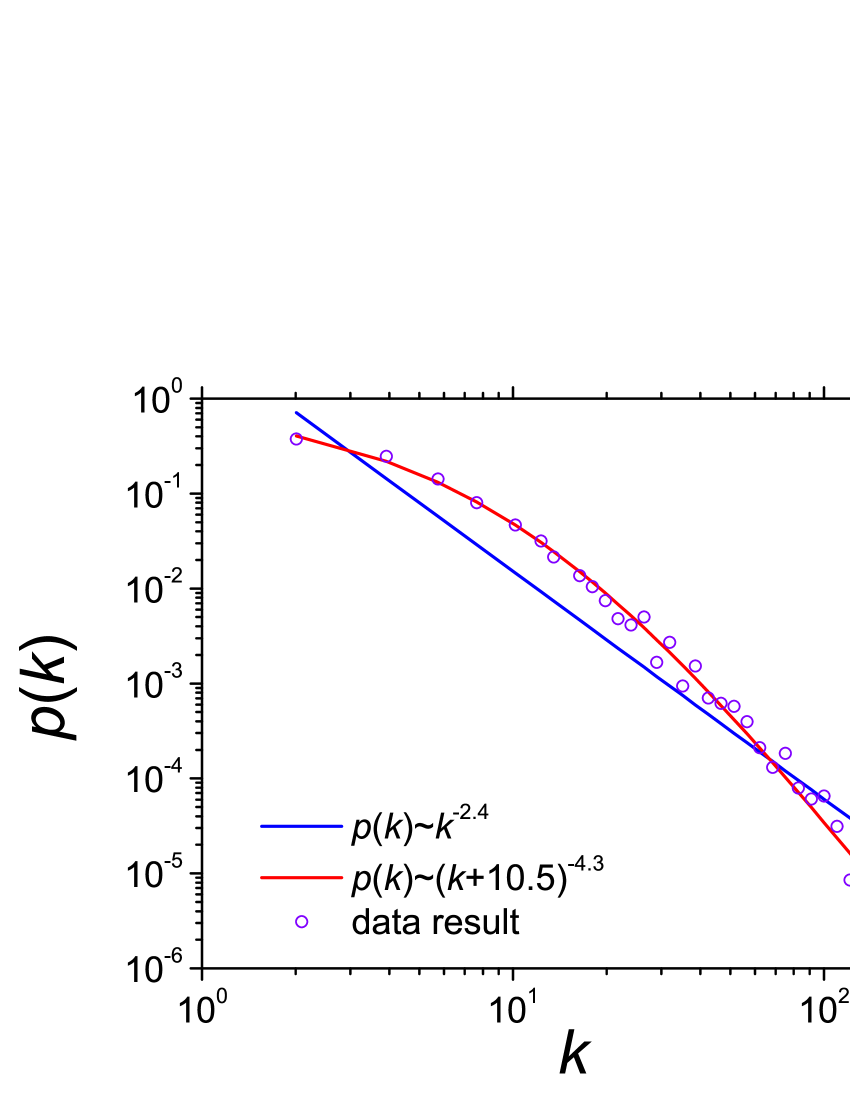
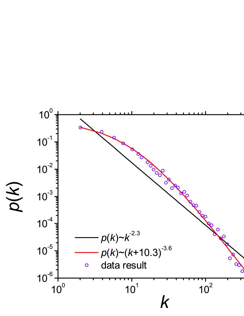
Figure 1: Illustration of power-law and Mandelbrot-law fittings for two scientific collaboration networks. The left and right plots respectively display the networks of smaller and larger sizes (i.e., SC-Small and SC-Large). Obviously, the Mandelbrot law performs much better.

Recently, the Mandelbrot law has been applied to characterize the degree distributions of some real networks Chang:2007 ; Wang:2009 . Here we test the validity of the Mandelbrot law on six real networks: (i) SC-Small.–A scientific collaboration network according to e-print manuscripts on condense matter physics from 1995 to 1999 in arxiv.org Newman:2001 ; (ii) SC-Large.–Similar to SC-Small but based on manuscripts published from 1993 to 2003 Leskovec2007 ; (iii) PPI.–A protein-protein interaction network of yeast Jeong2001 ; (iv) Slashdot.–A social network consisted of friend/foe links, attracted from the online service website, Slashdot Kunegis2009 . (v) USAir.–An air transportation network in the United States Colizza2007 . (vi) UCI.–A social network of students at University of California, Irvine Opsahl2009 . We try the least square method for both power law and Mandelbrot law, and the fitting exponents as well as square errors are shown in Table 1. From this table, we could conclude that: (i) Using the Mandelbrot law can generally improve the fitting accuracy compared with the power law since the former has one more coefficient; (ii) Sometimes the two fitting methods give more or less the same errors, and in these cases, the two power-law exponents are almost the same and the shifting coefficient is usually close to zero; (iii) Sometimes applying the Mandelbrot law can largely improve the fitting accuracy, and then the two power-law exponents are far different while the shifting coefficient is much larger than zero and its significant role cannot be neglected. Figure 1 displays the two cases with remarkable differences between two fitting methods, from which the advantage of the Mandelbrot law is demonstrated.

A number of tools have been developed to get the analytical solutions of network degree distributions, including the mean-field approximation, the master equation, the rate equation, and so on Barabasi:1999PhyA ; Dorogovtsev:2000 ; Krapivaky:2000 ; Zhou:2005 ; Moore:2006 . Most of these known analytical methods only concentrate on the power-law exponent, yet pay less attention to the value of shifting coefficient, which, however, plays a significant role in determining the shape of degree distributions (see figure 1). Even worse, we will show later that the widely used difference approximation, no matter forward difference or backward difference, will result in considerable deviations to the real value of the shifting coefficient.

We here investigate a model embodying a linear preferential attachment, which can be considered as an extension of the famous BA model. Initially, our model starts with a fully connected network with $m_{0}$ nodes and $m_{0}(m_{0}-1)/2$ links. If the final network size is $S$, it should satisfy the condition $m_{0}\ll S$. After initialization, at each time step, a new node will be added into the network, which will connect to $m$ old nodes. The probability of an old node $i$ to be connected is linearly correlated with its degree $k_{i}$, say

$$\Pi(k_{i})=\frac{1}{N}(\alpha k_{i}+\beta),$$ (5)

where $\alpha$ and $\beta$ are two parameters, and $N$ is the number of nodes at that time step. The self-loop and multiple links are not allowed. This model will degenerate to the BA model if $\beta=0$. The parameters $\alpha$ and $\beta$ satisfy the normalization condition

$$\sum_{k}\pi(k)p(k)=1,$$ (6)

where $\pi(k)=N\Pi(k)$ and $\pi(k)p(k)$ is the probability a selected old node is of degree $k$. That is

$$\sum_{k}\pi(k)p(k)=\sum_{k}(\alpha k+\beta)p(k)=2m\alpha+\beta=1.$$ (7)

It is equivalent to:

$$\alpha=\frac{1}{2m}(1-\beta).$$ (8)

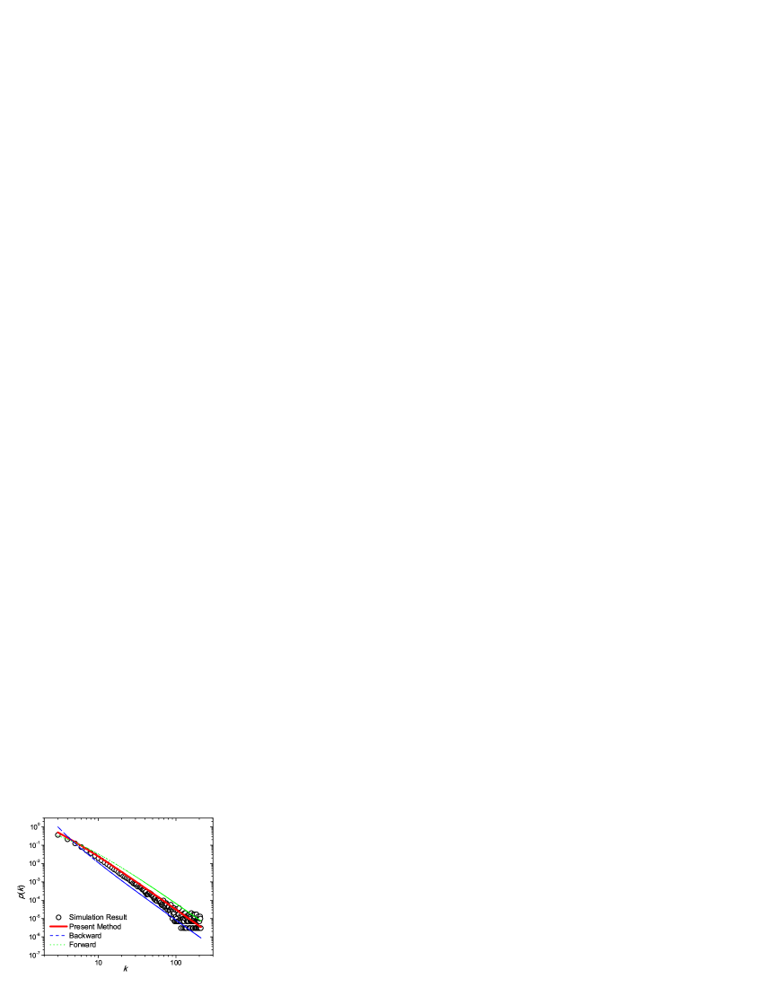
Figure 2: Degree distribution of the modeled network with $\beta=0$ and $m=3$. Since $\beta=0$, it is equivalent to a BA network. Compared with the results of backward difference approximation (blue dash line) and forward difference approximation (green dot line), the present solution (red solid line) is closer to the simulation result (round donuts). The network size is $S=10^{4}$ and the results are obtained by averaging over 100 independent realizations.

The rate equation is based on the assumption that the added nodes and links, during a time step, have no influence on the degree distribution of the network, namely in the thermodynamic limit, the degree distribution approaches to a steady form. Denoting $p(k)$ the steady degree distribution and $N$ the number of nodes in the current time step, if $N$ is large enough, then the number of nodes with degree $k$ is approximated to $Np(k)$. Analogously, the number of nodes with degree $k$ in the next step is $(N+1)p(k)$. With $m$ links added, the number of nodes with degree $k$ in the time step $N+1$ reads

$$(N+1)p(k)=Np(k)+m\pi(k-1)p(k-1)-m\pi(k)p(k)+\delta_{km},$$ (9)

where $m\pi(k-1)p(k-1)$ and $m\pi(k)p(k)$ represent, respectively, the number of nodes whose degree changes from $k-1$ to $k$ and from $k$ to $k+1$ in this time step. $\delta_{km}$ accounts for the specific degree equal to $m$, namely $\delta_{km}=1$ when $k=m$ and $\delta_{km}=0$ otherwise. Eq. (9) is the familiar form of the well-known rate equation Krapivaky:2000 ; Zhou:2005 , which is usually solved by the difference approximation, however, here we will show a different analytical method, and will later compare our results with the ones obtained by the difference approximation.

Eq. (9) is equivalent to

$$\begin{cases}p(m)=\frac{1}{1+m\pi(m)},k=m,\\ p(k)\left[1+m\pi(k)\right]=m\pi(k-1)p(k-1),k>m.\\ \end{cases}$$ (10)

Reminding the linear relation

$$\pi(k)=\alpha k+\beta,$$ (11)

considering Eq. (8), the probability of a newly added link connecting to an old node with minimum degree is

$$\pi(m)=\frac{1-\beta}{2m}m+\beta=\frac{1+\beta}{2}.$$ (12)

Clearly, this probability should be no less than zero and no larger than one, and thus $-1\leq\beta\leq 1$. According to Eq. (10), the probability density of $m$-degree nodes is

$$p(m)=\frac{1}{1+m\pi(m)}=\frac{2}{2+m(1+\beta)}.$$ (13)

Substituting Eq. (8) into Eq. (10), we get

$$p(k)\left[k+\frac{2(1+m\beta)}{1-\beta}\right]=\left[k+\frac{2m\beta}{1-\beta}-1\right]p(k-1).$$ (14)

Specifying:

$$a\equiv\frac{2m\beta}{1-\beta}-1,\texttt{ }b\equiv\frac{2(1+m\beta)}{1-\beta},$$ (15)

then Eq. (14) can be rewritten in a recursive formula as

$$p(k)=\frac{k+a}{k+b}p(k-1).$$ (16)

Taking logarithm in both sides of Eq. (16), we get

$$\log\frac{p(k)}{p(k-1)}=\log\frac{k+a}{k+b}.$$ (17)

With the ansatz that $p(k)$ follows the Mandelbrot law, substituting Eq. (3) into Eq. (17), we obtain the relationship between power-law exponent $\gamma$ and shifting coefficient $c$ as

$$\log\frac{k+a}{k+b}=\gamma\log\frac{k-1+c}{k+c},$$ (18)

which is equivalent to:

$$\log\frac{1+a\frac{1}{k}}{1+b\frac{1}{k}}=\gamma\log\frac{1+(c-1)\frac{1}{k}}{1+c\frac{1}{k}}.$$ (19)

Under the approximation with large $k$, through the second order Taylor expansion of Eq. (19) with $1/k$ being the variable, we can get the power-law exponent

$$\gamma=b-a=1+\frac{2}{1-\beta},$$ (20)

and the shifting coefficient

$$c=\frac{b+a+1}{2}=\frac{1+2m\beta}{1-\beta}.$$ (21)

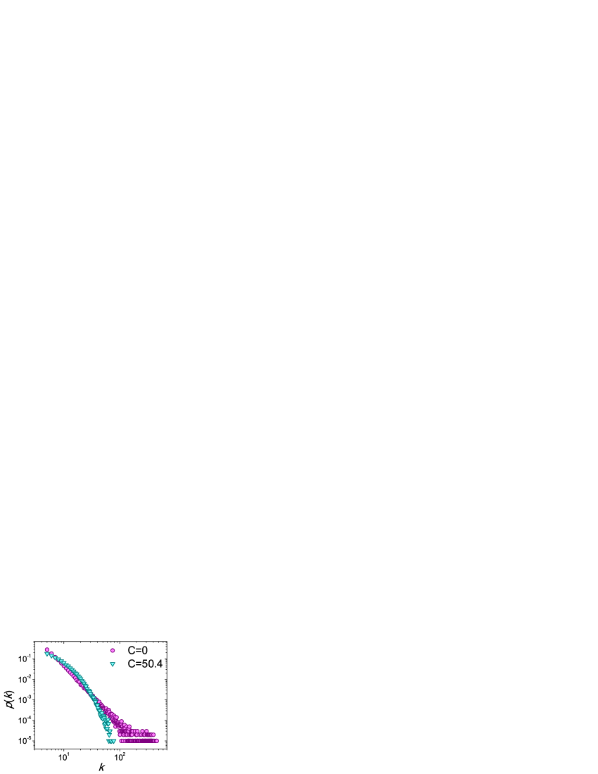
Figure 3: The comparison of degree distributions with different shifting coefficients given $m=5$ and $S=10000$. Compared with the case of $\beta=0.8$ and shifting coefficient $c=50.4$ (green down-triangles), the degree distribution of the none-shifting case with $\beta=-0.1$ and $c=0$ (purple circles) is much closer to a straight line in the log-log coordinates. The results are obtained by averaging over 100 independent realizations.

Eq. (20) and Eq. (21) declare that $\gamma$ only depends on $\beta$, while $c$ is related to both $\beta$ and $m$. When $m\beta$ is very large or $\beta\rightarrow 1$, $a$ and $b$ are both very large, and the Taylor expansion cannot be applied on Eq. (19). Under such condition, Eq. (16) can be approximately rewritten as

$$p(k)\approx\frac{a}{b}p(k-1),$$ (22)

then the degree distribution is close to an exponential form. It is easy to be understood since when $\beta\rightarrow 1$, the selection of old nodes is almost random. When $\beta=0$, $\alpha=\frac{1}{2m}$, our model degenerates to the BA model, and we get $a=-1$, $b=2$, $\gamma=3$ and $c=1$, with degree distribution being

$$p(k)=-\frac{2}{\psi(2,m+1)}(k+1)^{-3},$$ (23)

where

$$\psi(x)=\Gamma^{\prime}(x)/\Gamma(x)$$ (24)

is the Digamma function with

$$\Gamma(x)=\int_{0}^{\infty}e^{-t}t^{x-1}dt$$ (25)

being the Gamma function and

$$\psi(n,x)=\frac{d^{n}\psi(x)}{dx^{n}}.$$ (26)

We next compare the present method with methods based on the difference approximation. We first introduce the backward difference approximation, which assumes

$$\frac{dp}{dk}=p(k)-p(k-1).$$ (27)

Substituting Eq. (27) into Eq. (16), we get

$$p(k)=\frac{k+a}{k+b}\left[p(k)-\frac{dp}{dk}\right],$$ (28)

which is equivalent to

$$\frac{dp}{dk}=\frac{a-b}{k+a}p(k)$$ (29)

that leads to the solution

$$p(k)\propto(k+a)^{-(b-a)}.$$ (30)

Similarly, the forward difference approximation assumes

$$\frac{dp}{dk}=p(k+1)-p(k),$$ (31)

and then Eq. (16) can be rewritten as

$$p(k+1)=\frac{k+a+1}{k+b+1}p(k),$$ (32)

which is equivalent to

$$\frac{dp}{dk}=\frac{a-b}{k+1+b}p(k).$$ (33)

In this case, the solution is

$$p(k)\propto(k+b+1)^{-(b-a)}.$$ (34)

The three methods all indicate that the Mandelbrot law will emerge from an evolving network with linear preferential attachment, and give the same power-law exponent $\gamma=b-a$. In contrast, the shifting coefficient are different: $c^{\texttt{present}}=\frac{a+b+1}{2}$, $c^{\texttt{backward}}=a$ and $c^{\texttt{forward}}=b+1$. In Fig. 1, we compare the degree distributions obtained by these three methods with the simulation results and show that the present method is more accurate.

Although we usually refer to the concept of scale-free networks, neither the BA networks nor most real networks have very precisely power-law degree distributions. The present method suggests that we can obtain a more precisely power-law distribution by setting a right $\beta$ that corresponds to a zero shifting coefficient. Since the degree distribution is

$$p(k)\propto\left(k+\frac{1+2m\beta}{1-\beta}\right)^{1+\frac{2}{1-\beta}},$$ (35)

the non-shifted degree distribution asks for

$$c=\frac{1+2m\beta}{1-\beta}=0,$$ (36)

namely $\beta=-\frac{1}{2m}$ and $p(k)\propto k^{3-\frac{2}{2m+1}}$. Therefore, given the linear preferential attachment, the non-shifted power-law exponent is determined by the average degree and can never exceed 3. Figure 2 compares two degree distributions, respectively with $c=0$ and $c=50.4$, from which one can confirm that the non-shifted power law is indeed much closer to a straight line in the log-log coordinates, and the shifting coefficient largely affects the shape of degree distribution.

In summary, we extend the BA model to an evolving model with linear preferential attachment and show that the corresponding degree distribution obeys the Mandelbrot law. The shifting coefficient, usually being ignored in the literature, largely affects the shape of degree distribution. In puzzlement, the backward and forward difference approximations will lead to different solutions on shifting coefficient. Our analysis indicate that both of them are inaccurate, and we propose an analytical method that results in a more accurate solution.

References

- (1) S. H. Strogatz, Nature (London) 410, 268 (2001).
- (2) S. N. Dorogovtsev, Adv. Phys. 51, 1079 (2002).
- (3) R. Albert and A.-L. Barabási, Rev. Mod. Phys. 74, 47 (2002).
- (4) M. E. J. Newman, SIAM Rev. 167, 45 (2003).
- (5) D. J. Watts and S. H. Strogatz, Nature (London) 393, 440 (1998).
- (6) A.-L. Barabási and R. Albert, Science 286, 509 (1999).
- (7) A. L. Barabási, R. Albert, and H. Jeong, Physica A 272, 173 (1999).
- (8) M. E. J. Newman, Comtemporary Physics 46, 323 (2005).
- (9) A. Clauset, C. R. Shalizi, and M. E. J. Newman, SIAM Rev. 51, 661 (2009).
- (10) M. E. J. Newman, Proc. Natl. Acad. Sci. U.S.A. 98, 404 (2001).
- (11) M. E. J. Newman, S. Forrest, and J. Balthrop, Phys. Rev. E 66, 035101(R) (2002).
- (12) P.-P. Zhang, K. Chen, Y. He, T. Zhou, B.-B. Su, Y.-D. Jin, H. Chang, Y.-P. Zhou, L.-C. Sun, B.-H. Wang, and D.-R. He, Physica A 360, 599 (2006).
- (13) M.-S. Shang, L. Lü, Y.-C. Zhang, T. Zhou, Europhys. Lett. 90, 48006 (2010).
- (14) W. Li and X. Cai, Phys. Rev. E 69, 046106 (2004).
- (15) H.-K. Liu and T. Zhou, Acta Phys. Sin. 56, 106 (2007).
- (16) G. Bagler, Physica A 387, 2972 (2008).
- (17) B. Mandelbrot, Information theory and psycholinguistics (New York: Basic Books Publishing Co., 1965).
- (18) S. N. Dorogovtsev, J. F. F. Mendes, and A. N. Samukhin, Phys. Rev. Lett. 85, 4633 (2000).
- (19) H. Chang, B. B. Su, Y. P. Zhou, and D. R. He, Physica A 383, 687 (2007).
- (20) Y. L. Wang, T. Zhou, J. J. Shi, J. Wang, and D.-R. He, Physica A 388, 2949 (2009).
- (21) J. Leskovec, J. Kleinberg, and C. Faloutsos, ACM Trans. Knowl. Disc. from Data 1, 1 (2007).
- (22) H. Jeong, S. Mason, A.-L. Barabási, and Z. N. Oltvai, Nature 411, 41 (2001).
- (23) J. Kunegis, A. Lommatzsch, and C. Bauckhage, Proc. 18th Intl. Conf. WWW, ACM Press, 2009.
- (24) V. Colizza, R. Pastor-Satorras, and A. Vespignani, Nat. Phys. 3, 276 (2007).
- (25) T. Opsahl and P. Panzarasa, Social Networks 31, 155 (2009).
- (26) P. L. Krapivsky, S. Redner, and F. Leyvraz, Phys. Rev. Lett. 85, 4629 (2000).
- (27) T. Zhou, G. Yan, and B.-H. Wang, Phys. Rev. E 71, 046141 (2005).
- (28) C. Moore, G. Ghoshal, and M. E. J. Newman, Phys. Rev. E 74, 036121 (2006).