Approximate simulation of entanglement with a linear cost of communication

Abstract

Bell’s theorem implies that the outcomes of local measurements on two maximally entangled systems cannot be simulated without classical communication between the parties. The communication cost is finite for $n$ Bell states, but it grows exponentially in $n$. Three simple protocols are presented that provide approximate simulations for low-dimensional entangled systems and require a linearly growing amount of communication. We have tested them by performing some simulations for a family of measurements. The maximal error is less than $1\%$ in three dimensions and grows sublinearly with the number of entangled bits in the range numerically tested. One protocol is the multidimensional generalization of the exact Toner-Bacon [Phys. Rev. Lett. 91, 187904 (2003)] model for a single Bell state. The other two protocols are generalizations of an alternative exact model, which we derive from the Kochen-Specker [J. Math. Mech. 17, 59 (1967)] scheme for simulating single-qubit measurements. These protocols can give some indication for finding optimal one-way communication protocols that classically simulate entanglement and quantum channels. Furthermore they can be useful for deciding if a quantum communication protocol provides an advantage on classical protocols.

I Introduction

For some tasks in information processing, quantum communication channels were proved to be much more powerful than classical channels. While Holevo’s theorem holevo states that $n$ qubits cannot encode a message of more than $n$ classical bits, quantum channels reveal their real power when separate devices need to exchange information to jointly perform a task whose result depends on the data held by any single party. In distributed computing, the communication complexity of a problem is the cost in communication of the most efficient solution for that problem nisan . Similarly, the quantum communication complexity is the minimal amount of quantum communication required to accomplish a distributed computation. Quantum protocols for some communication problems, such as the Raz’s problem raz or the hidden matching (HM) problem baryossef , made clear that in some cases quantum channels can be exponentially more powerful than classical channels. Indeed, the HM problem exhibits an $n$ (qubits) versus $2^{\Omega(\sqrt{n})}$ (bits) gap between the quantum and classical communication complexity for bounded-error protocols. In the case of the Deutsch-Jozsa problem and errorless protocols, the gap is even stronger: $n$ qubits versus $\Omega(2^{n})$ bits buhrman0 . A review on quantum communication complexity can be found in Ref. buhrman .

A protocol of communication complexity is supposed to produce a correct result at least with high probability. Let us consider the scenario introduced by Yao yao . Two parties, say Alice and Bob, get a fixed part of the input data. Alice’s input is an element $m_{A}$ of a finite set $M_{A}$ and Bob’s input is an element $m_{B}$ of a finite set $M_{B}$. The purpose is computing a function $f(m_{A},m_{B})$ with a probability of success close to $1$ by some amount of communication between the parties. In a broader scenario one can just require that the outcome is generated according to a given probability distribution depending on $m_{A}$ and $m_{B}$. The problem of classically simulating a quantum communication channel fits into this extended framework. A quantum state is prepared by Alice through a procedure $m_{A}$ and sent to Bob through a quantum channel. He eventually performs a measurement through a procedure $m_{B}$. The measurement outcome, say $\beta$, is generated with a probability, $\rho(\beta|m_{A},m_{B})$, that depends on both $m_{A}$ and $m_{B}$. The task of a classical simulation is reproducing the distribution $\rho$ by replacing the quantum communication with a classical communication. This task is a particular problem of communication complexity in the outlined generalized sense. We call the minimal amount of classical communication needed in the simulation classical communication complexity of the quantum channel (the classical communication is not supposed to be necessarily one-way). Of course, such a simulation requires at least the same communication resources that are necessary for classically simulating a quantum communication protocol with an (almost) deterministic outcome. Thus, the previously mentioned results in quantum communication complexity sharpen the conceptual differences between quantum and classical physics. Indeed, they imply that any classical description of $n$ qubits requires a quantity of resources growing at least as $O(2^{n})$ brassard (or $2^{O(\sqrt{n})}$ if a bounded error is admitted), a property that hardly fits into the framework of classical physics, where in general the quantity of resources scales linearly with the amount of information virtually accessible in an experiment. Thus, a peculiar feature of quantum physics is the necessity of a huge quantity of information that is almost completely concealed from a direct experimental observation, but it is nevertheless fundamental in the description of systems. Indeed the whole information encoded in the quantum state cannot be used for carrying information holevo , but most of that is fundamental in the description of some quantum protocols of communication complexity.

There is an open question concerning the classical communication complexity of a quantum channel. On the one hand, the best known protocol for simulating a quantum channel uses an amount of resources that scales as $n2^{n}$ buhrman ; massar , even with a bounded error. On the other hand, the HM problem gives the lower bound $2^{\Omega(\sqrt{n})}$ for the minimal amount of communication in the case of bounded error. At present, no other constraint is known; thus one could hope to find a better bounded-error simulation of a quantum channel with communication complexity scaling as $2^{\sqrt{n}}$.

As established by Bell’s theorem bell , correlations of outcomes produced by local measurements on entangled systems cannot be explained classically without post-measurement communication between the parties. The problem of quantifying the classical communication complexity of a quantum channel of $n$ qubits is essentially equivalent to the problem of finding the minimal amount of communication needed to classically simulate the outcomes of local measurements on $n$ Bell states. Indeed classical protocols for simulating quantum channels can be converted into classical models of entanglement without affecting the cost of communication. Conversely, a classical model of entanglement can be converted into a model of quantum channels with a little more communication, as shown in Ref. cerf in the case of a single Bell state. A more general proof will be given in Sec. III.2, where we will show that an increase of communication by $n$ bits on average is sufficient for the conversion.

In this paper, we present three approximate classical protocols for simulating bipartite entanglement that need a one-way communication equal to the number of entangled bits (ebits). One of these is a multidimensional generalization of an exact model for a single ebit, reported by Toner and Bacon in Ref. toner . The other two protocols are generalizations of an alternative exact model, which will be derived here. The accuracy of the protocols was numerically tested for a family of measurements and for a dimension of the Hilbert space (of each party) between $2$ (one ebit) and $32$ ($5$ ebits). The maximum error is less than $1\%$ in the three-dimensional case and increases sublinearly with the number of ebits in the tested range (Note that the error cannot be bounded, since, as previously said, a protocol with bounded error needs at least $2^{O(\sqrt{n})}$ bits of communication). Our models can be useful for two reasons. First, they can give an indication for finding an optimal algorithm with bounded error, as discussed in the concluding remarks of the paper. Second, even if the maximal discrepancy increases with the number of qubits, these models or some modified version can give accurate results for measurements and states involved in some protocols of quantum communication complexity. In such a case they would give a proof that these quantum protocols do not provide any advantage on classical protocols.

In Sec. II, we review the Toner-Bacon protocol for a single Bell state and derive the alternative exact protocol starting from the Kochen-Specker hidden variable model of a qubit kochen . The three generalized protocols for higher dimensions of the Hilbert space and their Monte Carlo simulations are presented in Sec. III.1. In Sec. III.2 a general method for converting an entanglement model into a quantum channel model is presented. Finally, we draw the conclusions and perspectives in the last section.

II Simulation of Bell states with one bit of communication

Two qubits are prepared in the Bell state

$$|\Psi_{s}\rangle=\frac{1}{\sqrt{2}}\left(|1\rangle|2\rangle-|2\rangle|1\rangle\right)$$ (1)

and each one is sent to two parties, Alice and Bob, who perform a local measurement on their own qubit. Bell’s theorem bell implies that the outcome probabilities cannot be explained by a local classical theory and any exact simulation of this scenario needs some communication between the parties. How much information has to be exchanged? Trivially Bob could send the whole information about the measurement he performed, which is actually infinite. However, Brassard et al. brassard showed that a finite amount of communication is sufficient for exactly reproducing the outcome probabilities. They presented a model that simulates Bell correlations and requires exactly $8$ bits of communication. Steiner steiner reported a different model, which requires $2.97$ bits on average, but the amount of communication for each particular realization is unbounded. This result was improved in Ref. cerf , where the average information was lowered to $2.19$ bits. Later, Toner and Bacon showed that just one bit of communication can account for Bell correlations toner and two bits are sufficient for simulating teleportation of a qubit. In the next subsection we review this model. In Sec. II.2 an alternative exact model is derived whose direct generalization to $N$ dimensions is one of the three protocols described in Sec. III.1.

II.1 Toner-Bacon model

Let us consider the previously described scenario with two qubits in the Bell state (1). Alice and Bob perform two projective measurements. Bob’s measurement projects the quantum state into one of two mutually orthogonal vectors of the two-dimensional Hilbert space. Let us represent them by the Bloch vectors $\vec{b}_{1}$ and $\vec{b}_{2}=-\vec{b}_{1}$. Alice performs a projective measurement on the states $\vec{a}_{1}$ and $\vec{a}_{2}=-\vec{a}_{1}$. The joint probability of having outcomes $\vec{a}_{\alpha}$ and $\vec{b}_{\beta}$ is

$$P(\alpha,\beta)=\frac{1}{4}\left(1-\vec{a}_{\alpha}\cdot\vec{b}_{\beta}\right).$$ (2)

It is possible to exactly reproduce this statistics through a classical protocol that uses just one bit of classical communication. The protocol is as follows. Alice and Bob share two random unit vectors $\vec{\lambda}_{1}$ and $\vec{\lambda}_{2}$. They are uncorrelated and uniformly distributed on the unit sphere. Bob generates the outcome $\beta$ such that the vector $\vec{b}_{\beta}\in\{\vec{b}_{1},\vec{b}_{2}\}$ is closest to $\vec{\lambda}_{1}$, that is,

$$\mathrm{sgn}(\vec{b}_{\beta}\cdot\vec{\lambda}_{1})>0.$$ (3)

Bob sends one bit $n\in\{-1,1\}$ to Alice, where

$$n=\mathrm{sgn}(\vec{b}_{\beta}\cdot\vec{\lambda}_{2}).$$ (4)

Alice generates the outcome $\alpha$ such that

$$\mathrm{sgn}\left[\vec{a}_{\alpha}\cdot(\vec{\lambda}_{1}+n\vec{\lambda}_{2})\right]<0.$$ (5)

This protocol produces the events according to the quantum probability $P(\alpha,\beta)$, as proved in Ref. toner . Note that the effect of $n$ is to change the sign of $\vec{\lambda}_{2}$, that is, Alice receives the instruction “if $n$ is negative, flip the vector $\vec{\lambda}_{2}$ to the opposite direction”.

It is useful to express the protocol in a form that is trivial to generalize to higher dimensions of the Hilbert space. For this purpose we replace the Bloch vectors with vectors in the two-dimensional Hilbert space. While the state (1) simplifies the notation with Bloch vectors, for a generalization to higher dimensions it is better to use the state

$$|\Psi\rangle=\frac{1}{\sqrt{2}}\left(|1\rangle|1\rangle+|2\rangle|2\rangle\right).$$ (6)

The two states (1,6) differ by the local unitary transformation $e^{i\frac{\pi}{2}\hat{\sigma}_{y}^{(2)}}$, performed on the second qubit.

The projective measurements are represented by two sets of orthogonal vectors,

$$\{|\phi_{1}\rangle,|\phi_{2}\rangle\}\equiv M_{A},\;\;\{|\psi_{1}\rangle,|\psi_{2}\rangle\}\equiv M_{B}$$ (7)

Alice and Bob measure $M_{A}$ and $M_{B}$, respectively. Each vector in the set is associated with one outcome. In the simulation, the shared vector $\vec{\lambda}_{1}$ is replaced by a vector $|x\rangle$ in the two-dimensional Hilbert space,

$$\vec{\lambda}_{1}\rightarrow|x\rangle,$$ (8)

so that $\vec{\lambda}_{1}$ is the Bloch vector of $|x\rangle$. The vector $\vec{\lambda}_{2}$ is replaced by a set of orthogonal vectors in the Hilbert space,

$$\vec{\lambda}_{2}\rightarrow\{|y_{1}\rangle,|y_{2}\rangle\},$$ (9)

so that $\vec{\lambda}_{2}$ and $-\vec{\lambda}_{2}$ are the Bloch vectors of $|y_{1}\rangle$ and $|y_{2}\rangle$, respectively. In this new frame, the Toner-Bacon protocol is as follows. According to Eq. (3), Bob generates the outcome $|\psi_{\beta}\rangle\in M_{B}$ that is closest to $|x\rangle$ (he maximizes $|\langle\psi_{\beta}|x\rangle|^{2}$). Then he sends Alice the index $n\in\{1,2\}$ such that $|y_{n}\rangle\in\{|y_{1}\rangle,|y_{2}\rangle\}$ is the vector closest to $|\psi_{\beta}\rangle$ [from Eq. (4)]. Let us introduce the vector

$$|\phi_{k}^{*}\rangle\equiv\langle\phi_{k}|1\rangle|1\rangle+\langle\phi_{k}|2\rangle|2\rangle$$ (10)

for $k=1,2$. It is obtained from $|\phi_{k}\rangle$ by the complex conjugation of the coefficients in the basis $\{|1\rangle,|2\rangle\}$. Alice generates the outcome $|\phi_{\alpha}\rangle\in M_{A}$ that maximizes the function

$$\langle\phi_{\alpha}^{*}|\left\{|x\rangle\langle x|+|y_{n}\rangle\langle y_{n}|\right\}|\phi_{\alpha}^{*}\rangle.$$

Note that Eq. (5) would ask to minimize $\langle\phi_{\alpha}|\left\{|x\rangle\langle x|+|y_{n}\rangle\langle y_{n}|\right\}|\phi_{\alpha}\rangle$ in the case of state (1). It is easy to show that for state (6) “minimization” is replaced by “maximization” and $|\phi_{\alpha}\rangle$ by $|\phi_{\alpha}^{*}\rangle$. The outcomes are generated according to Born’s rule, that is,

$$P(\alpha,\beta|M_{A},M_{B})=\frac{1}{2}|\langle\phi_{\alpha}|\psi_{\beta}\rangle|^{2}.$$ (11)

This new reformulation of the Toner-Bacon protocol suggests a very simple generalization to higher dimensions of the Hilbert space, as discussed in Sec. III.1.

II.2 Alternative model

An alternative exact classical model for a Bell state can be obtained from the hidden variable model of a qubit introduced by Kochen and Specker (KS)kochen . This can be seen as a classical model of a quantum channel where the communicated classical information is infinite and encoded in a three-dimensional unit vector. It can be transformed into a model with finite communication cost, as shown below.

II.2.1 Quantum channel

Let us introduce the KS model. It provides a classical simulation of the following scenario. Bob prepares a qubit in a quantum state represented by a Bloch vector $\vec{b}$. He sends the qubit to Alice, who performs a projective measurement $M_{A}=\{\vec{a}_{1},\vec{a}_{2}\}$ with outcome states $\vec{a}_{1}$ and $\vec{a}_{2}\equiv-\vec{a}_{1}$. The classical simulation is as follows. Given the Bloch vector $\vec{b}$, Bob generates a unit vector $\vec{x}_{1}$ with probability

$$\rho(\vec{x}_{1}|\vec{b})=\frac{1}{\pi}\vec{b}\cdot\vec{x}_{1}\theta(\vec{b}\cdot\vec{x}_{1}),$$ (12)

where $\theta(z)$ is the Heaviside function, which is equal to $1$ if $z>0$ and zero otherwise. He sends $\vec{x}_{1}$ to Alice. Given the vector pair $M_{A}=\{\vec{a}_{1},\vec{a}_{2}\}$, Alice generates the outcome $\vec{a}_{\alpha}$ according to the conditional probability

$$P(\alpha|\vec{x}_{1};M_{A})=\theta(\vec{a}_{\alpha}\cdot\vec{x}_{1});$$ (13)

in other words, she generates deterministically the vector closest to $\vec{x}_{1}$. This model gives the correct quantum probability for the outcomes, that is,

$$\int d^{2}x_{1}P(\alpha|\vec{x}_{1};M_{A})\rho(\vec{x}_{1}|\vec{b})=\frac{1}{2}\left(1+\vec{a}_{\alpha}\cdot\vec{b}\right).$$ (14)

Let us define the vectors

$$\begin{array}[]{l}\vec{y}_{1}\equiv\vec{x}_{1}+\vec{x}_{2},\\ \vec{y}_{2}\equiv\vec{x}_{1}-\vec{x}_{2}.\end{array}$$ (15)

It is easy to show that the probability distribution (12) can be obtained from the uniform distribution

$$\rho(\vec{x}_{1},\vec{x}_{2}|\vec{b})=\frac{1}{4\pi^{2}}\theta(\vec{b}\cdot\vec{y}_{1})\theta(\vec{b}\cdot\vec{y}_{2})$$ (16)

by integrating out the unit vector $\vec{x}_{2}$. The integration is trivial in spherical coordinates and is left as an exercise. This uniform probability distribution and the conditional probability (13) still give the correct quantum predictions. More generally we get an exact simulation of a qubit with the probability distributions

$$\rho(\vec{x}_{1},\vec{x}_{2}|n_{1},n_{2};\vec{b})=\frac{1}{4\pi^{2}}\theta\left(n_{1}\vec{b}\cdot\vec{y}_{1}\right)\theta\left(n_{2}\vec{b}\cdot\vec{y}_{2}\right)$$ (17)

$$P(\alpha|\vec{x}_{1},\vec{x}_{2},n_{1},n_{2};M_{A})=\theta\left[\vec{a}_{\alpha}\cdot(n_{1}\vec{y}_{1}+n_{2}\vec{y}_{2})\right]$$ (18)

for any $n_{i}=\pm 1$. For example, with $n_{1}=1$ and $n_{2}=-1$, Eqs. (17, 18) can be derived from Eqs. (13,16) by exchanging $\vec{x}_{1}$ and $\vec{x}_{2}$. With $n_{1}=-1$ and $n_{2}=-1$ we have to flip the direction of $\vec{x}_{1}$ and $\vec{x}_{2}$. Finally, with $n_{1}=-1$ and $n_{2}=1$ we have to exchange and flip the vectors.

Suppose that the indices $n_{i}$ are randomly generated with probability $\rho_{I}(n_{1},n_{2})\equiv 1/4$. The joint probability distribution of $\vec{x}_{i}$ and $n_{i}$ can be suitably written in the form

$$\rho(\vec{x}_{1},\vec{x}_{2},n_{1},n_{2}|\vec{b})=\rho(n_{1},n_{2}|\vec{x}_{1},\vec{x}_{2};\vec{b})\rho_{v}(\vec{x}_{1},\vec{x}_{2}),$$ (19)

where

$$\rho(n_{1},n_{2}|\vec{x}_{1},\vec{x}_{2};\vec{b})\equiv\theta\left(n_{1}\vec{b}\cdot\vec{y}_{1}\right)\theta\left(n_{2}\vec{b}\cdot\vec{y}_{2}\right)$$ (20)

and

$$\rho_{v}(\vec{x}_{1},\vec{x}_{2})\equiv\frac{1}{(4\pi)^{2}}.$$ (21)

The model with probability distribution (19) and conditional probability (18) gives again the correct quantum probabilities, but now we have the nice property that the marginal probability distribution $\rho_{v}(\vec{x}_{1},\vec{x}_{2})$ of the vectors $\vec{x}_{1}$ and $\vec{x}_{2}$ does not depend on the prepared quantum state $\vec{b}$. This dependence is only in the conditional probability distribution $\rho(n_{1},n_{2}|\vec{x}_{1},\vec{x}_{2};\vec{b})$ of the discrete indices $n_{i}$. This reformulation of the Kochen-Specker model gives a protocol with shared noise for simulating the communication of a qubit with just two bits of classical communication: Bob and Alice share the random vectors $\vec{x}_{1}$ and $\vec{x}_{2}$, generated according to the uniform probability distribution (21); given a quantum state $\vec{b}$, Bob generates the discrete indices $n_{i}$ according to rule (20); he sends them to Alice; given a measurement $M_{A}$, Alice generates the outcome $\vec{a}_{\alpha}$ according to rule (18).

II.2.2 Entanglement

Any classical simulation of a quantum channel can be converted into a simulation of entanglement without increasing the amount of communication. Consider again the scenario of Sec. II.1 with two qubits in the Bell state (1). Alice and Bob perform two projective measurements, $M_{A}=\{\vec{a}_{1},\vec{a}_{2}\}$ and $M_{B}=\{\vec{b}_{1},\vec{b}_{2}\}$, respectively, and get outcomes $\vec{a}_{\alpha}$ and $\vec{b}_{\beta}$. The marginal probability of $\beta$ is uniformly distributed on the values $1$ and $2$. Furthermore, given Bob’s outcome $\vec{b}_{\beta}$, Alice’s outcome is generated as if she received the quantum state $-\vec{b}_{\beta}$ directly from Bob. Thus, the joint probability distribution of the outcomes can be simulated as follows. Bob randomly generates the outcome $\vec{b}_{\beta}$ with uniform probability distribution $\rho(\beta)=1/2$. He then uses a classical model of a quantum channel for sending the quantum state $-\vec{b}_{\beta}$ to Alice, who finally generates her own outcome $\vec{a}_{\alpha}$. The amount of communication of the derived entanglement model is equal to that of the quantum channel model.

The classical model of a quantum channel previously derived from the KS model gives the following protocol for simulating entanglement. Alice and Bob share the random vectors, $\vec{x}_{1}$ and $\vec{x}_{2}$, and perform two projective measurements, $M_{A}=\{\vec{a}_{1},\vec{a}_{2}\}$ and $M_{B}=\{\vec{b}_{1},\vec{b}_{2}\}$, respectively. Bob generates the outcome $\vec{b}_{\beta}$ and the indices $n_{1}=\pm 1$, $n_{2}=\pm 1$ according to the probability distribution

$$\rho(\beta,n_{1},n_{2}|\vec{x}_{1},\vec{x}_{2};M_{B})\equiv\frac{1}{2}\theta\left(n_{1}\,\vec{b}_{\beta}\cdot\vec{y}_{1}\right)\theta\left(n_{2}\,\vec{b}_{\beta}\cdot\vec{y}_{2}\right),$$

He sends $n_{i}$ to Alice. She generates the outcome $\vec{a}_{\alpha}$ according to the probability distribution defined by Eq. (18).

In this model the amount of communication is $2$ bits. It is possible to reduce the communication cost by means of the transformation $n_{1}\vec{y}_{1}\rightarrow\vec{y}_{1}$. Indeed the index $n_{1}$ becomes uncorrelated with the other variables and can be eliminated. Thus, we get a model with a communication cost of $1$ bit, defined by the conditional probabilities

$$\rho(\beta,n|\vec{x}_{1},\vec{x}_{2};M_{B})\equiv\theta\left(\vec{b}_{\beta}\cdot\vec{y}_{1}\right)\theta\left(n\,\vec{b}_{\beta}\cdot\vec{y}_{2}\right),$$ (22)

$$\rho(\alpha|\vec{x}_{1},\vec{x}_{2},n;M_{A})=\theta\left[-\vec{a}_{\alpha}\cdot(\vec{y}_{1}+n\vec{y}_{2})\right].$$ (23)

That is, Bob generates the vector $\vec{b}_{\beta}$ closest to $\vec{y}_{1}$ and sets the discrete index $n$ equal to the sign of $\vec{b}_{\beta}\cdot\vec{y}_{2}$. He sends $n$ to Alice. She then generates the outcome $\vec{a}_{\alpha}$ that is closest to $\vec{y}_{1}+n\vec{y}_{2}$. Note that this model is very similar to the Toner-Bacon model, with the only difference that the unit vectors $\vec{x}_{i}$ are replaced by the vectors $\vec{y}_{i}$, which are a linear combination of $\vec{x}_{i}$ [see Eq. (15)].

This model of entanglement can be put into a more synthetic form that will be useful in Sec. III.1. Suppose that the measurement outcomes are $\vec{a}_{\bar{\alpha}}$ and $\vec{b}_{\bar{\beta}}$ and the communicated index is $\bar{n}$; then it is easy to show by Eq. (22) that $\vec{b}_{\bar{\beta}}\cdot\vec{x}_{\bar{n}}\geq\vec{b}_{\beta}\cdot\vec{x}_{n}$ for any $\beta\in\{1,2\}$ and $n\in\{1,2\}$. Furthermore from Eq. (23) we have that $-\vec{a}_{\bar{\alpha}}\cdot\vec{x}_{\bar{n}}\geq-\vec{a}_{\alpha}\cdot\vec{x}_{\bar{n}}$ for any $\alpha\in\{1,2\}$. Thus, the algorithm can be reformulated as follows. Bob evaluates the vectors $\vec{b}_{\beta}\in\{\vec{b}_{1},\vec{b}_{2}\}$ and $\vec{x}_{n}\in\{\vec{x}_{1},\vec{x}_{2}\}$ that maximize $\vec{b}_{\beta}\cdot\vec{x}_{n}$. He generates the outcome $\vec{b}_{\beta}$ and sends the index $n=\{1,2\}$ to Alice. Alice generates the outcome $\vec{a}_{\alpha}\in\{\vec{a}_{1},\vec{a}_{2}\}$ that maximizes $-\vec{a}_{\alpha}\cdot\vec{x}_{n}$. This algorithm will be generalized to higher dimensions of the Hilbert space in the next section.

III Generalizing to higher dimensions

In Sec. III.1 the three approximate protocols for simulating entanglement in higher dimensions are introduced. In Sec. III.2 we will present a simple method for converting an entanglement protocol into a protocol for simulating quantum channels.

III.1 Entanglement

Let us consider the following scenario. Alice and Bob receive two $N$-dimensional quantum systems in the entangled state

$$|\psi_{AB}\rangle=\frac{1}{\sqrt{N}}\sum_{k=1}^{N}|k\rangle_{A}|k\rangle_{B}$$ (24)

They perform local projective measurements using the set of orthogonal vectors $\{|\phi_{1}\rangle,...,|\phi_{N}\rangle\}\equiv M_{A}$ and $\{|\psi_{1}\rangle,...,|\psi_{N}\rangle\}\equiv M_{B}$, respectively. This scenario can be reproduced by local hidden variables augmented by some amount of communication.

The gap between the classical and quantum algorithms in the HM problem implies that this communication cannot be smaller than $e^{O(\sqrt{n})}$ in the case of bounded error, $n=\log_{2}N$ being the number of ebits. A stronger constraint was given in Ref. brassard , where it was shown that $O(2^{n})$ bits of communication are necessary for an exact simulation. An exact two-way classical protocol with $O(n2^{n})$ bits of communication on average was reported by Massar et al. massar . Unlike the protocols considered in this paper, the protocol in Ref. massar does not require any local hidden variables. A one-way model of a quantum channel for a single qubit was recently reported in Ref. montina0 . It requires an infinite amount of communication for an exact simulation, but it has the nice property of encoding the communication in a single real variable, instead of two real variables, which are required for defining a quantum state. It can be easily converted into a classical protocol of entanglement. Just as that in Ref. massar , this protocol does not need local hidden variables.

In this section we present three approximate protocols for simulating entanglement that give accurate results for low values of $N$ and require a communication of just $n$ bits. They were numerically tested for a family of measurements. The maximal discrepancy between the best protocol and the quantum predictions is less than $1\%$ for $N=3$ and grows sublinearly with $n(=\log_{2}N)$ in the range numerically studied. The first protocol is a generalization of the Toner-Bacon model of a single Bell state, suitably readjusted in Sec. II.1. The second protocol is a generalization of the alternative model presented in Sec. II.2. The last model is similar to the second one, but with a different shared randomness.

Protocol $1$

1. Bob and Alice share one random vector $|x\rangle$ and a random basis $\{|y_{1}\rangle,...,|y_{N}\rangle\}\equiv Y$.

2. Bob generates the outcome $|\psi_{b}\rangle\in M_{B}$ that is closest to $|x\rangle$.

3. He sends Alice the index of the vector $|y_{m}\rangle\in Y$ that is closest to $|\psi_{b}\rangle$.

4. Alice generates the event $|\phi_{a}\rangle\in M_{A}$ that maximizes $\langle\phi_{a}^{*}|\left\{|x\rangle\langle x|+|y_{n}\rangle\langle y_{n}|\right\}|\phi_{a}^{*}\rangle$, where $|\phi_{a}^{*}\rangle\equiv\sum_{k}\langle\phi_{a}|k\rangle|k\rangle$.

Note that this model gives the right marginal distributions for the outcomes of each party, since the vectors $|x\rangle$ and $|y_{k}\rangle$ are generated uniformly in the Hilbert space. This holds also for the other protocols. Thus, only the accuracy of the correlations has to be checked.

Protocol $2a$

1. Bob and Alice share a set $R\equiv\{|x_{1}\rangle,...,|x_{N}\rangle\}$ of $N$ random vectors.

2. Bob evaluates the vectors $|\psi_{b}\rangle\in M_{B}$ and $|x_{n}\rangle\in R$ that maximize $|\langle\psi_{b}|x_{n}\rangle|^{2}$.

3. He generates the outcome $|\psi_{b}\rangle$ and sends $n$ to Alice.

4. Alice generates the event $|\phi_{a}\rangle\in M_{A}$ that maximizes $|\langle\phi_{a}^{*}|x_{n}\rangle|^{2}$.

This protocol is the generalization of the classical model of entanglement derived in Sec. II.2. As shown below, it is more accurate than protocol $1$ for $N\geq 10$, in the sense that the maximal discrepancy (in the set of tested measurements) is lower. This is true at least for $N\leq 32$, which is the maximal dimension we considered in the numerical simulations. The last protocol is similar to protocol $2a$, but the vectors $|x_{k}\rangle$ are orthogonal.

Protocol $2b$: the same as protocol $2a$, but Bob and Alice share a random orthogonal basis.

While this protocol is not exact for $N=2$, it is more accurate than protocol $2a$ for $N>2$. As shown by the numerical simulations, the accuracies of protocols $2a$ and $2b$ approach each other in the limit of high dimensions.

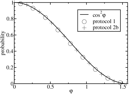
Figure 1: Probability of the event $|\phi_{1}\rangle$ given $|\psi_{1}\rangle$ as a function of $\varphi$ for $N=3$. The solid line is the quantum prediction. The circles and crosses are the probabilities obtained from protocols $1$ and $2b$, respectively.

It is interesting to note that the three protocols share a common feature. Kochen and Specker proved that any deterministic hidden variable theory equivalent to quantum theory is contextual kochen . Although our protocols are not completely equivalent to quantum theory, they satisfy this general constraint, that is, the probability of a joint event $(|\phi_{\alpha}\rangle,|\psi_{\beta}\rangle)$ depends on the whole set of orthogonal vectors $M_{A}$ and $M_{B}$. Indeed, all the vectors in the sets are involved in the maximization procedures used by the protocols. It is interesting to note that a similar procedure of maximization was used in an approximate hidden-variable model of qutrit reported in Ref. rudolph . The Kochen-Specker theorem was recently generalized to probabilistic theories in Ref. montina .

Since these protocols are contextual and approximate, we can expect that the probability distribution of two events $|\psi_{\beta}\rangle$ and $|\phi_{\alpha}\rangle$ again depends on all the vectors in the sets $M_{A}$ and $M_{B}$. For the sake of simplicity, here we will consider the set of one-parameter measurements

$$\begin{array}[]{l}|\phi_{1}\rangle=\cos\varphi|\psi_{1}\rangle-\sin\varphi|\psi_{2}\rangle,\\ |\phi_{2}\rangle=\sin\varphi|\psi_{1}\rangle+\cos\varphi|\psi_{2}\rangle,\\ |\phi_{k}\rangle=|\psi_{k}\rangle\;\mathrm{for}\;k=3,...,N,\end{array}$$ (25)

that is, the vectors $|\phi_{k}\rangle$ are set equal to $|\psi_{k}\rangle$ for $k>2$. The results do not change qualitatively with a different choice of the measurements.

The quantum probabilities of the joint events $|\phi_{b}\rangle$ and $|\psi_{a}\rangle$ for $a\neq 1,2$ or $b\neq 1,2$ are obviously equal to $\delta_{a,b}$. The probabilities $P(a,b|\varphi)$ of the outcomes $a=1,2$ and $b=1,2$, given $\varphi$, are

$$P(1,1|\varphi)=P(2,2|\varphi)=\frac{1}{N}\cos^{2}\varphi$$ (26)

$$P(1,2|\varphi)=P(2,1|\varphi)=\frac{1}{N}\sin^{2}\varphi.$$ (27)

Note that the measurement with $\varphi=\varphi_{0}$ is equivalent to the measurement with $\varphi=\frac{\pi}{2}-\varphi_{0}$ and $|\psi_{1}\rangle$ and $|\psi_{2}\rangle$ swapped. Furthermore, $\sum_{k,l}P(k,l|\varphi)=1$. Thus, it is sufficient to evaluate the discrepancy between the model and quantum theory for outcomes $a=b=1$ and $\varphi=[0,\pi/2]$. This discrepancy contains the full information about the discrepancy of any other event with constraint (25).

In Fig. 1, we report the probability of an event $|\phi_{1}\rangle$, given $|\psi_{1}\rangle$, as a function of $\varphi$ for $N=3$. The solid line is the quantum prediction $\cos^{2}\varphi$. The circles and crosses are the Monte Carlo results, generated by the protocols $1$ and $2b$. The maximal discrepancy between protocol $2b$ and $\cos^{2}\varphi$ is very small, less than $0.01$, and is barely perceptible in the figure. Protocol $2a$ gives the worst results with a maximal discrepancy about $0.025$. Its data are not reported in the figure. The maximal discrepancy for protocol $1$ is about $0.014$. The numerical simulations were performed with $10^{7}$ Monte Carlo executions, which make the statistical error inappreciable in the figure.

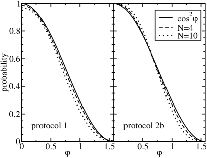
Figure 2: Same as Fig. 1 with $N=4$ (dashed line) and $N=10$ (dotted line).

The same simulations were executed for higher dimensions of the Hilbert space; the results for $N=4$ (two qubits) and $N=10$ are plotted in Fig. 2. The probabilities generated by protocol $1$($2b$) are reported at the left-hand (right-hand) side. It is interesting to note that protocol $2b$ gives the right probability for $\varphi=0,\pi/2$, that is, when $|\phi_{1}\rangle$ and $|\psi_{1}\rangle$ are parallel or orthogonal. However, a small discrepancy was noted for measurements that do not satisfy constraint (25).

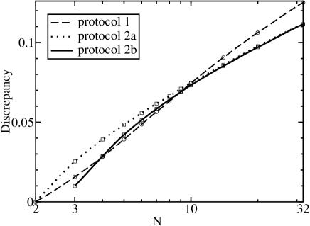
Figure 3: Maximum discrepancy between the quantum prediction and the classical protocols as a function of $N$. The data are interpolated by lines, plotted as a guide of eyes.

The maximum discrepancy of the three protocols is reported in Fig. 3 as a function of $N$. The horizontal axis is in logarithmic scale. For large values of $N$, protocols $2a$ and $2b$ have the same discrepancy. This is because in protocol $1$ the vectors $|x_{k}\rangle$, which are generated randomly, have a very high probability of being almost orthogonal to each other for $N\gg 1$. This fact makes protocol $2a$ almost indistinguishable from protocol $2b$ in high dimensions.

III.2 Quantum channel

In Ref. cerf it was shown that any protocol that simulates entanglement of two qubits can be converted into a classical model of a quantum channel for a single qubit. A very simple method for converting a general classical model of entanglement into a classical model of a quantum channel is as follows. In the entanglement model, Bob and Alice share a set $R$ of random vectors. This means that they have a common list of noise realizations $R_{k}$, with $k=1,2,3,...$. They start from $k=1$ and at each execution of the Monte Carlo simulation they read the next element of the list. It is possible to convert the protocol into a protocol for simulating quantum channels by increasing the communication by $n$ bits on average. Suppose that Bob receives the quantum state $|\psi\rangle$. He selects a measurement $M_{B}$={$|\psi_{1}\rangle$,…,$|\psi_{N}\rangle$} so that $|\psi_{1}\rangle=|\psi\rangle$. Using the protocol for simulating entanglement and the first noise realization in the shared list, Bob generates a vector $|\psi_{b}\rangle$. If $|\psi_{b}\rangle\neq|\psi\rangle$, Bob interrupts the protocol for simulating entanglement and reads the next realization of the noise in the shared list; he repeats the procedure until $|\psi_{b}\rangle=|\psi\rangle$. He then executes the communication procedure as established by the entanglement protocol. Furthermore he sends the number of noise realizations that Alice has to skip. This additional information is equal to $\log_{2}N=n$ on average.

Thus, using this strategy, it is possible to convert the three models of entanglement into protocols for simulating quantum channels. This conversion requires doubling the amount of communication on average.

IV Conclusion

In this paper we have presented three approximate one-way communication protocols for simulating the outcomes of local measurements, performed on bipartite entangled states. These protocols use an amount of communication equal to the number $n$ of ebits. We have seen that they can be converted into approximate protocols for simulating quantum communication channels. Approximate models like these can be useful for detecting if a quantum communication algorithm can be efficiently simulated by some classical algorithm. This is the case when a quantum communication algorithm uses states and measurements that an approximate model of a quantum channel can efficiently simulate with zero or bounded error in any dimension.

The results reported in this paper can be improved in different ways. It is interesting to note that the protocols $2a$ and $2b$ have the same general structure, but different shared noises. The general structure is as follows. Bob and Alice share a set $R\equiv\{|x_{1}\rangle,...,|x_{N}\rangle\}$ of $N$ random vectors with probability distribution $\rho(|x_{1}\rangle,...,|x_{N}\rangle)$. Bob evaluates the vectors $|\psi_{b}\rangle\in M_{B}$ and $|x_{n}\rangle\in R$ that maximize the function

$$F_{1}(b,n)\equiv|\langle\psi_{b}|x_{n}\rangle|^{2}.$$ (28)

He generates the outcome $|\psi_{b}\rangle$ and sends $n$ to Alice. Alice generates the event $|\phi_{a}\rangle\in M_{A}$ that maximizes the function

$$F_{2}(a)\equiv|\langle\phi_{a}^{*}|x_{n}\rangle|^{2}.$$ (29)

We have seen that a suitable choice of the noise distribution can considerably reduce the error. Indeed, in the three-dimensional case a change of noise dropped the error from $2.5\%$ (protocol $2a$) to less than $1\%$ (protocol $2b$).

Thus, protocols $2a$ and $2b$ can be improved by evaluating the optimal probability distribution $\rho(|x_{1}\rangle,...,|x_{N}\rangle)$ that minimizes the maximal or average error over a set of measurements. Of course, the error cannot be reduced to zero if the whole set of measurements is considered, since this would require an exponential amount of communication. However, another possible improvement can be reached by augmenting the communication cost, namely $\log_{2}N$. This is achieved by increasing the number $N$ of random vectors $|x_{k}\rangle$. We can expect that this strategy and the optimal choice of $\rho$ will enhance the accuracy of the model, as defined through the functions in Eqs. (28,29). For a sufficiently large amount of communication, one can hope to make the error bounded. Notice that, as said in the introduction, the HM problem establishes the lower bound $2^{(\Omega(\sqrt{n})}$ for the communication cost, whereas the best known protocols require an amount of communication that scales as $n2^{n}$ buhrman ; massar . At present it is not clear if such protocols are also optimal. This open problem can be investigated by studying the class of protocols introduced in this paper. In conclusion, our models can give some indication for finding optimal one-way communication protocols that classically simulate quantum channels and entanglement. Furthermore, they can be used for testing the efficiency of a quantum communication protocol versus classical protocols.

References

- (1) A. S. Holevo, Probl. Peredachi Inf. 9, 3 (1973) [Probl. Inf. Transm. 9, 177 (1973)].
- (2) E. Kushilevitz and N. Nisan, “Communication complexity”, (Cambridge University Press, 1997).
- (3) R. Raz, Proceedings of 31st ACM STOC, pages 358-367 (1999).
- (4) Z. Bar-Yossef, T. S. Jayram, and I. Kerenidis, Proceedings of 36th ACM STOC, pages 128-137 (2004).
- (5) H. Buhrman, R. Cleve, A. Wigderson, Proceedings of 30th ACM STOC, 63 (1998).
- (6) H. Buhrman et al., Rev. Mod. Phys. 82, 665 (2010).
- (7) A. C. Yao, Proc. of 11th STOC 14, 209 (1979).
- (8) G. Brassard, R. Cleve, A. Tapp, Phys. Rev. Lett. 83, 1874 (1999).
- (9) S. Massar et al., Phys. Rev. A 63, 052305 (2001).
- (10) J. S. Bell, Physics (Long Island City, N.Y.) 1, 195 (1964).
- (11) N. J. Cerf, N. Gisin, S. Massar, Phys. Rev. Lett. 84, 2521 (2000).
- (12) B. F. Toner and D. Bacon, Phys. Rev. Lett. 91, 187904 (2003).
- (13) S. Kochen and E. Specker, J. Math. Mech. 17, 59 (1967).
- (14) M. Steiner, Phys. Lett. A 270, 239 (2000).
- (15) A. Montina, Phys. Lett. A 375, 1385 (2011).
- (16) T. Rudolph, arXiv:quant-ph/0608120.
- (17) Z. Chen and A. Montina, Phys. Rev. A 83, 042110 (2011).