Abstract. We introduce an algorithm that iteratively produces a sequence of natural numbers $k_{i}$ and functions $b_{i}$ defined in the interval $[1,+\infty)$. The number $k_{i+1}$ arises as the first point of discontinuity of $b_{i}$ above $k_{i}$. We derive a set of properties of both sequences, suggesting that (1) the algorithm produces square-free numbers $k_{i}$, (2) all the square-free numbers are generated as the output of the algorithm, and (3) the value of the Möbius function $\mu(k_{i})$ can be evaluated as $b_{i}(k_{i+1})-b_{i}(k_{i})$. The logical equivalence of these properties is rigorously proved. The question remains open if one of these properties can be derived from the definition of the algorithm. Numerical evidence, limited to $5\times 10^{6}$, seems to support this conjecture.

Keywords: Möbius function, square-free numbers, zeta function, Riemann hypothesis.

AMS Subject Classification: 11Y55, 11M99, 11Y35.

1 Introduction

A natural number $n\in\mathbb{N}$ is called square-free, if the exponents arising in its prime factorization

$$n=p_{1}^{r_{1}}\,p_{2}^{r_{2}}\cdots p_{k}^{r_{k}}$$

are all equal to 1, i.e., $r_{1}=r_{2}=\cdots=r_{k}=1$. For a natural number $n$ with prime factorization as above, the Möbius function $\mu$ is defined as

$$\mu(n)=\begin{cases}1&\text{if $n=1$;}\\ (-1)^{\sum_{i=1}^{k}r_{i}},&\text{if $n$ is square-free;}\\ 0,&\text{otherwise.}\end{cases}$$

In other words, $\mu(n)$ is zero when $n$ has a square factor, and otherwise gives the parity of the number of (distinct) prime factors of $n$. The Möbius function has important applications in number theory, many of them concerning to the Riemann hypothesis about the zeros of the zeta function, [1], [6], [7], [8].

An outstanding problem in algorithmic number theory is to compute $\mu(n)$ efficiently without first factoring $n$. By “efficiently” we mean a number of bit operations bounded by a polynomial in $\log n$, the length of $n$ in binary. As far as we know, the question remains open if the computation of $\mu(n)$ can be done in polynomial time, and in fact, nobody currently knows a way to compute it significantly faster than factoring $n$.

In this paper, we present an algorithm that iteratively produces a sequence of numbers $k_{i}$ and the value of $\mu(k_{i})$. In order to determine $\mu(k_{i})$, it is necessary to generate the whole sequence $k_{1},k_{2},\dots,k_{i}$. Our algorithm is based on a sequence of arithmetical functions $b_{i}$, with the numbers $k_{i}$ arising as discontinuity points. These functions are closely related to the Nyman-Beurling approach to the Riemann hypothesis. The main result of the present paper is a set of properties of the sequences $k_{i}$ and $b_{i}$, suggesting that

• The numbers $k_{i}$ generated by the algorithm are square-free.

• The set of all the square-free numbers can be generated by the algorithm.

• The value of the Möbius function $\mu(k_{i})$ can be evaluated as $b_{i}(k_{i+1})-b_{i}(k_{i})$.

We are able to prove the logical equivalence of these properties. Unfortunately, using the definition of the algorithm, we cannot prove, neither disprove, if one (then all) of these conditions are satisfied. Numerical evidence, limited to $5\times 10^{6}$, seems to support the conjectures quoted above.

This paper is organized as follows. The section 2 introduces the framework of the Nyman-Beurling approach to Riemann hypothesis. The section 3 provides the basic definitions for this paper, and the algorithm is defined in section 4. The main result of the present work is stated and proved in section 5, while further remarks are done in section 6. Finally, the implementation of the algorithm and numerical results are discussed in section 7.

2 Hilbert Space Approach to Riemann Hypothesis

Denote by $\left\lfloor{x}\right\rfloor$ the integer part of $x$, i.e., the greatest integer less than, or equal to, $x$. Define the fractional part function by $\left\{{x}\right\}=x-\left\lfloor{x}\right\rfloor$. Given $n\in\mathbb{N}$ and two families of parameters $\{a_{k}\}_{k=1}^{n}\subset\mathbb{C}$ and $\{\theta_{k}\}_{k=1}^{n}\subset(0,1]$, we define a Beurling function as a function $F_{n}$ (the sub-index $n$ included in the notation for convenience) of the form

$$F_{n}(x)\,\,\textrm{\raisebox{1.5pt}{\defi:}=}\,\sum_{k=1}^{n}a_{k}\,\left\{{\frac{\theta_{k}}{x}}\right\}.$$ (1)

For a Beurling function $F_{n}$, an elementary computation shows that

$$\int_{0}^{1}(F_{n}(x)+1)\,x^{s-1}\,dx=\frac{\displaystyle\sum_{k=1}^{n}a_{k}\,\theta_{k}}{s-1}+\frac{1}{s}\left(1-\zeta(s)\,\sum_{k=1}^{n}a_{k}\,\theta_{k}^{s}\right);$$ (2)

for the complex variable $s\in\mathbb{C}$ in the half-plane $\operatorname{Re}(s)>0$, i.e. for $s$ with positive real part. Here, $\zeta$ denotes the Riemann’s zeta function given by

$$\zeta(s)\,\,\textrm{\raisebox{1.5pt}{\defi:}=}\,\sum_{k=1}^{\infty}\frac{1}{k^{s}}.$$

The classic references are [8] and [6]. A derivation of the relation (2) can be found, for instance, in [2, p. 253]. It is useful (but not always necessary from a theoretical point of view) to assume that the parameters defining the function $F_{n}$ satisfy the additional condition

$$\sum_{k=1}^{n}a_{k}\,\theta_{k}=0.$$ (3)

In this case, the first term at the right-hand side of (2) vanishes, simplifying the expression. The identity (2) is the starting point of the following theorem by Beurling

Theorem 1 (Beurling).

The zeta function $\zeta(s)$ has no zeros in the half-plane $\operatorname{Re}(s)>1/p$ if and only if the set of (Beurling) functions $\{f_{\theta}(x)=\left\{{\theta/x}\right\}\}_{0<\theta\leqslant 1}$ is dense in $L^{p}([0,1],dx)$.

See [2, p. 252] for a proof of the Beurling theorem and further references. Note that for $p=2$ this result provides an equivalent condition to the Riemann hypothesis (RH) for the zeta function. This is the Beurling, or Nyman-Beurling, approach to RH.

The Beurling theorem above has an easy half part, whose proof can be sketched as follows. From relation (2) and assuming (3), we have

$$\left|{\frac{1}{s}\left(1-\zeta(s)\,\sum_{k=1}^{n}a_{k}\,\theta_{k}^{s}\right)}\right|=\left|{\int_{0}^{1}(F_{n}(x)+1)\,x^{s-1}\,dx}\right|\leqslant\left\|{F_{n}(x)+1}\right\|\,\left\|{x^{s-1}}\right\|;$$

where the last relation follows using the Schwarz inequality in $L^{2}([0,1],dx)$. Therefore, if the first norm in the right-hand side above can be done arbitrarily small for a suitable choice of $n$, $a_{k}$’s and $\theta_{k}$’s, then the function $\zeta(s)$ could not have zeros for $\operatorname{Re}(s)>1/2$. We will refer to the first condition above as the Beurling criterion (BC) for RH. Note also that in order to demonstrate the RH, it is sufficient to prove that the constant function equal to $-1$ can be arbitrarily approximated in the norm of the Hilbert space $L^{2}([0,1],dx)$ by Beurling functions $F_{n}$ of the form (1). It was proved in [4] that BC remains equivalent to RH if the parameters $\theta_{k}$ are restricted to be reciprocal of natural numbers, i.e. $\theta_{k}=1/b_{k}$, with $b_{k}\in\mathbb{N}$.

Several approximating functions to $-1$ of the form (1) were proposed in the literature. From the relations (2) and (3), we have that under the BC, the “partial sum”

$$\sum_{k=1}^{n}a_{k}\,\theta_{k}^{s}.$$ (4)

is an approximation to the reciprocal of the zeta function $1/\zeta(s)$, which is known to have an expression as a Dirichlet series

$$\frac{1}{\zeta(s)}\;=\;\sum_{k=1}^{n}\frac{\mu(k)}{k^{s}},$$ (5)

convergent for $\operatorname{Re}(s)>1$. Therefore, a (naive) first choice for an approximating function would be

$$S_{n}(x)\,\,\textrm{\raisebox{1.5pt}{\defi:}=}\,\sum_{k=1}^{n}\mu(k)\,\left\{{\frac{1/k}{x}}\right\}.$$ (6)

Note that this function does not matches the condition (3). We can handle this without subtlety, just by subtracting the difference, that is given by $g(n)$, where

$$g(t)\,\,\textrm{\raisebox{1.5pt}{\defi:}=}\,\sum_{\mathbb{N}\ni k\leqslant t}\frac{\mu(k)}{k}.$$ (7)

Therefore, a second choice would be

$$B_{n}(x) \,\,\textrm{\raisebox{1.5pt}{\defi:}=}\,\sum_{k=1}^{n}\mu(k)\,\left\{{\frac{1/k}{x}}\right\}\;-\;n\,g(n)\,\left\{{\frac{1/n}{x}}\right\}$$ (8)

$$\,\,\textrm{\phantom{\raisebox{1.5pt}{\defi:}}=}\,\sum_{k=1}^{n-1}\mu(k)\,\left\{{\frac{1/k}{x}}\right\}\;-\;n\,g(n-1)\,\left\{{\frac{1/n}{x}}\right\}.$$ (9)

Other variants were also proposed, as

$$V_{n}(x)\,\,\textrm{\raisebox{1.5pt}{\defi:}=}\,\sum_{k=1}^{n}\mu(k)\,\left\{{\frac{1/k}{x}}\right\}\;-\;g(n)\,\left\{{\frac{1}{x}}\right\}.$$ (10)

Unfortunately, the sequences (6), (9) and (10) are known to be not convergent to $-1$ in $L^{2}([0,1],dx)$, as proved in [3]. A survey on the Nyman-Beurling reformulation of the Riemann hypothesis and later developments by Baez-Duarte can be found in [5].

3 Basic Definitions

In order to motivate the definitions below, assume that a Beurling function $F_{n}$ as in (1) is constant between the reciprocal of the natural numbers. In other words, assume that such a function takes a constant value in each of the intervals $(\frac{1}{k+1},\frac{1}{k}]$, for all $k\in\mathbb{N}$ (but the constant value may differ from interval to interval). In this case, the integral in (2) can be expressed alternatively as an infinite series, involving the values of $f_{n}(k)\,\,\textrm{\raisebox{1.5pt}{\defi:}=}\,F_{n}(1/k)$. Furthermore, the values of $F_{n}(x)$ for all $x\in[0,1]$ are completely determined by the values of $f_{n}(k)$ for all $k\in\mathbb{N}$. We will call an arithmetical Beurling function a function of the form $f_{n}(k)=F_{n}(1/k)$, where $F_{n}$ is a Beurling function.

We introduce now, perhaps the simplest, non-trivial, example of arithmetical Beurling function satisfying the condition (3). For $a,b\in\mathbb{N}$ define the function $\beta_{a,b}$ as

$$\beta_{a,b}(x)\,\,\textrm{\raisebox{1.5pt}{\defi:}=}\,\left\{{\frac{x}{{a}}}\right\}\;-\;\frac{{b}}{{a}}\,\left\{{\frac{x}{{b}}}\right\},$$ (11)

As the functions $\beta_{a,b}$ will be the basic blocks in our construction, we summarize some of its elementary properties in the following result.

Lemma 1.

Consider $a,b\in\mathbb{R}$, with $0<a<b$. Then,

• $\displaystyle{\left\{{\frac{x}{a}}\right\}}$ and $\displaystyle{\left\{{\frac{x}{b}}\right\}}$ are right-continuous, and linearly independent functions.

• $\beta_{a,b}(x)=0$, when $0\leqslant x<a$.

• Let $k\in\mathbb{N}$ be such that $(k-1)a<b\leqslant ka$. Then,

  $$\beta_{a,b}(x)=\begin{cases}-j&\text{\rm if $ja\leqslant x<(j+1)a$, for $j=1,\dots,(k-2)$;}\\ -(k-1)&\text{\rm if $(k-1)a\leqslant x<b$.}\end{cases}$$

• Assume $a,b\in\mathbb{N}$. Then, $\beta_{a,b}(x)$ is constant when $k\leqslant x<k+1$, for all $k\in\mathbb{N}$.

Proof:

(a): The right-continuity is derived from of $\left\lfloor{x}\right\rfloor$. Now, if $c_{1}\,\left\{{\frac{x}{a}}\right\}\;+\;c_{2}\,\left\{{\frac{x}{b}}\right\}=0$ for all $x$, then for $x=a$ we have $0=c_{1}\,\left\{{\frac{a}{a}}\right\}\;+\;c_{2}\,\left\{{\frac{a}{b}}\right\}=c_{2}\,\frac{a}{b}$. Thus, $c_{2}=0$ and we have $c_{1}\,\left\{{\frac{x}{a}}\right\}=0$ for all $x$, and taking now $x=a/2$ we get $0=c_{1}\,\left\{{\frac{1}{2}}\right\}=c_{1}/2$ and $c_{1}=0$.

(b): If $0\leqslant x<a<b$, then $x/b<1$ and $x/a<1$. Thus, $\left\{{\frac{x}{a}}\right\}-\frac{b}{a}\left\{{\frac{x}{b}}\right\}=\frac{x}{a}-\frac{b}{a}\frac{x}{b}=0$.

(c): Assume $j=1,\dots,(k-2)$. Then, for $ja\leqslant x<(j+1)a<b$, we have $x/b<1$ and $j\leqslant x/a<(j+1)$. Thus, $\left\{{\frac{x}{a}}\right\}-\frac{b}{a}\left\{{\frac{x}{b}}\right\}=\frac{x}{a}-\left\lfloor{\frac{x}{a}}\right\rfloor-\frac{b}{a}\frac{x}{b}=\frac{x}{a}-j-\frac{x}{a}=-j$. Analogously, for $(k-1)a\leqslant x<b<ka$, we have $x/b<1$ and $(k-1)\leqslant x/a<k$. Thus, $\left\{{\frac{x}{a}}\right\}-\frac{b}{a}\left\{{\frac{x}{b}}\right\}=\frac{x}{a}-\left\lfloor{\frac{x}{a}}\right\rfloor-\frac{b}{a}\frac{x}{b}=\frac{x}{a}-(k-1)-\frac{x}{a}=-(k-1)$.

(d): If $x<b$ then (d) is true by (b) and (c) already proven. Consider now $b\leqslant x$. If $k<x<k+1$ then $x\notin\mathbb{N}$ and thus $x/a\notin\mathbb{N}$ and $x/b\notin\mathbb{N}$. Therefore, there exists $k_{0}$ and $l_{0}$ in $\mathbb{N}$ such that $ak_{0}<x<a(k_{0}+1)$ and $bl_{0}<x<b(l_{0}+1)$, and we have $\left\{{\frac{x}{a}}\right\}-\frac{b}{a}\left\{{\frac{x}{b}}\right\}=\frac{x}{a}-k_{0}-\frac{b}{a}(\frac{x}{b}-l_{0})=-k_{0}+\frac{b}{a}l_{0}$, which is a constant independent of $x$. As $\left\{{\frac{x}{a}}\right\}-\frac{b}{a}\left\{{\frac{x}{b}}\right\}$ is right-continuous, by part (a), this is also true for $k\leqslant x<k+1$.  

4 The Algorithm

We will define a sequence of numbers $\{k_{i}\}_{i\in\mathbb{N}}$ and functions $\{b_{i}\}_{i\in\mathbb{N}}$ iteratively as follows. Start with the following definitions

$$\begin{split}k_{1}&\,\,\textrm{\raisebox{1.5pt}{\defi:}=}\,1;\\ k_{2}&\,\,\textrm{\raisebox{1.5pt}{\defi:}=}\,2;\\ b_{2}(x)&\,\,\textrm{\raisebox{1.5pt}{\defi:}=}\,\left\{{\frac{x}{k_{1}}}\right\}\;-\;\frac{k_{2}}{k_{1}}\,\left\{{\frac{x}{k_{2}}}\right\}.\end{split}$$ (12)

Assuming now that $k_{i}$ and $b_{i}$ are already defined, for $i\geqslant 2$ define iteratively $k_{i+1}$ and $b_{i+1}$ as follows. The number $k_{i+1}$ is defined as $k_{i+1}\,\,\textrm{\raisebox{1.5pt}{\defi:}=}\,k_{i}+j$, where $j$ is the least integer such that $b_{i}(k_{i}+j)\neq b_{i}(k_{i})$. Once determined the number $k_{i+1}$, the function $b_{i+1}$ is defined as

$$b_{i+1}(x)\,\,\textrm{\raisebox{1.5pt}{\defi:}=}\,b_{i}(x)\;+\;\left(1+b_{i}(k_{i})\right)\left(\left\{{\frac{x}{k_{i}}}\right\}\;-\;\frac{k_{i+1}}{k_{i}}\,\left\{{\frac{x}{k_{i+1}}}\right\}\right).$$ (13)

Some elementary properties derived from these definitions are summarized in the following result.

Lemma 2.

For any $i\in\mathbb{N}$ we have

• $b_{i}$ is a right-continuous function, which is constant between the natural numbers.

• $b_{i+1}(k_{i})=-1$.

• Assume $k_{i+1}\leqslant 2k_{i}$ for $i\geqslant 2$. Then, $b_{i}(x)=-1$ for all $x\in[1,k_{i})$. In particular, the sequence $\{b_{i}\}_{i\in\mathbb{N}}$ converges point-wise to $-1$ in $[1,+\infty)$.

Proof:

(a): Observe that each $b_{i}$ is a (finite) linear combination of $\beta_{p,q}$. Therefore, this result is a direct consequence of Lemma 1.

(b): Is an immediate consequence of definition (13).

(c): For induction on $i$. The case $i=2$ is an immediate consequence of definition (12). Assume now that $b_{j}(x)=-1$ when $x\in[1,k_{j})$ for all $j\leqslant i$. If $x<k_{i}<k_{i+1}$, then from definition (13) we have $b_{i+1}(x)=b_{i}(x)$ which is equal to $-1$ by the inductive hypothesis. Now if $k_{i}\leqslant x<k_{i+1}\leqslant 2k_{i}$, also from definition (13) we have

$$b_{i+1}(x)=b_{i}(x)+(1+b_{i}(k_{i}))\,\left(\frac{x}{k_{i}}-1-\frac{k_{i+1}}{k_{i}}\,\frac{x}{k_{i+1}}\right)=b_{i}(x)-1-b_{i}(k_{i})=-1,$$

because by the definition of $k_{i+1}$, the function $b_{i}(x)$ is constant for $x\in[k_{i},k_{i+1})$.  

Remark:

As $b_{i}$ is a constant function between the natural numbers, the number $k_{i+1}$ is the first point of discontinuity of $b_{i}$ above $k_{i}$.

5 Main Result

The next result is relevant in order to establish a relationship between the sequence $\{k_{i}\}_{i\in\mathbb{N}}$, the values of $\mu(k_{i})$, and the square-free numbers.

Lemma 3.

The following conditions are equivalent

• $\displaystyle{\sum_{j=1}^{i}\frac{\mu(k_{j})}{k_{j}}\;=\;\frac{1+b_{i}(k_{i})}{k_{i}}}$, for $i\geqslant 2$.

• $\displaystyle{b_{i}(x)=\sum_{j=1}^{i-1}\mu(k_{j})\,\left\{{\frac{x}{k_{j}}}\right\}\;-\;k_{i}\left(\sum_{j=1}^{i-1}\frac{\mu(k_{j})}{k_{j}}\right)\left\{{\frac{x}{k_{i}}}\right\}}$, for $i\geqslant 2$.

• $\displaystyle{\frac{\mu(k_{i})}{k_{i}}=\frac{1+b_{i}(k_{i})}{k_{i}}\;-\;\frac{1+b_{i-1}(k_{i-1})}{k_{i-1}}}$, for $i\geqslant 3$.

Furthermore, if the condition $k_{i+1}<2k_{i}$ is valid for $i\geqslant 2$, then all conditions above are also equivalent to the following ones

• $\displaystyle{\mu(k_{i+1})=b_{i}(k_{i+1})\;-\;b_{i}(k_{i})}$, for $i\geqslant 2$.

• $\displaystyle{\sum_{j=1}^{i}\mu(k_{j})\left\lfloor{\frac{k_{i}}{k_{j}}}\right\rfloor=1}$, for $i\geqslant 1$.

Proof:

In order to prove the logical equivalence between all conditions in Lemma 3, we separately will prove, first of all, the equivalences (a)$\Leftrightarrow$(b) and (a)$\Leftrightarrow$(c). Then, after the introduction of the additional condition $k_{i+1}<2k_{i}$, we will prove the equivalence between (d)$\Leftrightarrow$(c) and (e)$\Leftrightarrow$(b).

(a)$\Rightarrow$(b): For induction on $i$. For $i=2$, from definition (12) we have

$$b_{2}(x)=\left\{{\frac{x}{k_{1}}}\right\}-\frac{k_{2}}{k_{1}}\,\left\{{\frac{x}{k_{2}}}\right\}=\mu(k_{1})\,\left\{{\frac{x}{k_{1}}}\right\}-k_{2}\,\frac{\mu(k_{1})}{k_{1}}\,\left\{{\frac{x}{k_{2}}}\right\}.$$ (14)

Assuming now that condition (b) follows for all $j$ such that $j\leqslant i$, we have

$$b_{i+1}(x)=b_{i}(x)+\left(1+b_{i}(k_{i})\right)\left(\left\{{\frac{x}{k_{i}}}\right\}-\frac{k_{i+1}}{k_{i}}\,\left\{{\frac{x}{k_{i+1}}}\right\}\right)\\ =\sum_{j=1}^{i-1}\mu(k_{j})\,\left\{{\frac{x}{k_{j}}}\right\}-k_{i}\left(\sum_{j=1}^{i-1}\frac{\mu(k_{j})}{k_{j}}\right)\left\{{\frac{x}{k_{i}}}\right\}+\left(1+b_{i}(k_{i})\right)\left(\left\{{\frac{x}{k_{i}}}\right\}-\frac{k_{i+1}}{k_{i}}\,\left\{{\frac{x}{k_{i+1}}}\right\}\right)\\ =\sum_{j=1}^{i-1}\mu(k_{j})\,\left\{{\frac{x}{k_{j}}}\right\}-k_{i}\left(\sum_{j=1}^{i-1}\frac{\mu(k_{j})}{k_{j}}\right)\left\{{\frac{x}{k_{i}}}\right\}+\left(k_{i}\sum_{j=1}^{i}\frac{\mu(k_{j})}{k_{j}}\right)\left(\left\{{\frac{x}{k_{i}}}\right\}-\frac{k_{i+1}}{k_{i}}\,\left\{{\frac{x}{k_{i+1}}}\right\}\right)\\ =\sum_{j=1}^{i-1}\mu(k_{j})\,\left\{{\frac{x}{k_{j}}}\right\}-k_{i}\left(\sum_{j=1}^{i-1}\frac{\mu(k_{j})}{k_{j}}\right)\left\{{\frac{x}{k_{i}}}\right\}\hfill\\ \hfill+k_{i}\left(\sum_{j=1}^{i}\frac{\mu(k_{j})}{k_{j}}\right)\left\{{\frac{x}{k_{i}}}\right\}-k_{i+1}\left(\sum_{j=1}^{i}\frac{\mu(k_{j})}{k_{j}}\right)\left\{{\frac{x}{k_{i+1}}}\right\}\\ =\sum_{j=1}^{i-1}\mu(k_{j})\,\left\{{\frac{x}{k_{j}}}\right\}+k_{i}\,\frac{\mu(k_{i})}{k_{i}}\,\left\{{\frac{x}{k_{i}}}\right\}-k_{i+1}\left(\sum_{j=1}^{i}\frac{\mu(k_{j})}{k_{j}}\right)\left\{{\frac{x}{k_{i+1}}}\right\}\\ =\sum_{j=1}^{i}\mu(k_{j})\,\left\{{\frac{x}{k_{j}}}\right\}-k_{i+1}\left(\sum_{j=1}^{i}\frac{\mu(k_{j})}{k_{j}}\right)\left\{{\frac{x}{k_{i+1}}}\right\};$$ (15)

and this proves condition (b) for $i+1$. Here, in the first equality we have used the inductive hypothesis and in the second one we have used condition (a).

(b)$\Rightarrow$(a): From Lemma 2 (b), by condition (b) we have

$$\begin{split}0&=1+b_{i+1}(k_{i})\\ &=1+\sum_{j=1}^{i}\mu(k_{j})\,\left\{{\frac{k_{i}}{k_{j}}}\right\}-k_{i+1}\left(\sum_{j=1}^{i}\frac{\mu(k_{j})}{k_{j}}\right)\left\{{\frac{k_{i}}{k_{i+1}}}\right\}\\ &=1+\sum_{j=1}^{i-1}\mu(k_{j})\,\left\{{\frac{k_{i}}{k_{j}}}\right\}+\mu(k_{i})\,\left\{{\frac{k_{i}}{k_{i}}}\right\}-k_{i+1}\left(\sum_{j=1}^{i}\frac{\mu(k_{j})}{k_{j}}\right)\frac{k_{i}}{k_{i+1}}\\ &=1+\sum_{j=1}^{i-1}\mu(k_{j})\,\left\{{\frac{k_{i}}{k_{j}}}\right\}-k_{i}\left(\sum_{j=1}^{i}\frac{\mu(k_{j})}{k_{j}}\right)\\ &=1+b_{i}(k_{i})-k_{i}\left(\sum_{j=1}^{i}\frac{\mu(k_{j})}{k_{j}}\right);\end{split}$$ (16)

and this proves condition (a). Here we have used that $\left\{{\frac{k_{i}}{k_{i+1}}}\right\}=\frac{k_{i}}{k_{i+1}}$, (because $\frac{k_{i}}{k_{i+1}}<1$), that $\left\{{\frac{k_{i}}{k_{i}}}\right\}=0$, and also the relation $b_{i}(k_{i})=\sum_{j=1}^{i-1}\mu(k_{j})\,\left\{{\frac{k_{i}}{k_{j}}}\right\}$, which is an easy consequence of condition (b).

(a)$\Rightarrow$(c): Using condition (a) for $i$ and $i-1$ we have

$$\sum_{j=1}^{i}\frac{\mu(k_{j})}{k_{j}} =\frac{1+b_{i}(k_{i})}{k_{i}},$$ (17)

$$\sum_{j=1}^{i-1}\frac{\mu(k_{j})}{k_{j}} =\frac{1+b_{i-1}(k_{i-1})}{k_{i-1}};$$ (18)

and subtracting (18) from (17) we get condition (c).

(c)$\Rightarrow$(a): Denoting $\alpha(i)\,\,\textrm{\raisebox{1.5pt}{\defi:}=}\,\frac{1+b_{i}(k_{i})}{k_{i}}$, from (c) we have

$$\sum_{j=1}^{i}\frac{\mu(k_{j})}{k_{j}}=\frac{\mu(k_{1})}{k_{1}}\;+\;\frac{\mu(k_{2})}{k_{2}}\;+\;\sum_{j=3}^{i}\alpha(j)-\alpha(j-1)\;=\;1\;-\;\frac{1}{2}\;+\;\alpha(i)-\alpha(2)\\ =\;1\;-\;\frac{1}{2}\;+\;\alpha(i)\;-\;\frac{1+b_{2}(k_{2})}{k_{2}}\;=\;1\;-\;\frac{1}{2}\;+\;\alpha(i)\;-\;\frac{1}{2}\;=\;\alpha(i)\;=\;\frac{1+b_{i}(k_{i})}{k_{i}}.$$ (19)

Here we have used that $b_{2}(k_{2})=0$, by definition (12).

Therefore, we have proved (b)$\Leftrightarrow$(a)$\Leftrightarrow$(c). Assume now condition $k_{i+1}<2k_{i}$, for $i\geqslant 2$.

(d)$\Leftrightarrow$(c): From definition (13) we have

$$\begin{split}b_{i}(k_{i})&=b_{i-1}(k_{i})+\left(1+b_{i-1}(k_{i-1})\right)\left(\left\{{\frac{k_{i}}{k_{i-1}}}\right\}-\frac{k_{i}}{k_{i-1}}\,\left\{{\frac{k_{i}}{k_{i}}}\right\}\right)\\ &=b_{i-1}(k_{i})+\left(1+b_{i-1}(k_{i-1})\right)\,\left\{{\frac{k_{i}}{k_{i-1}}}\right\}\\ &=b_{i-1}(k_{i})+\left(1+b_{i-1}(k_{i-1})\right)\left(\frac{k_{i}}{k_{i-1}}-\left\lfloor{\frac{k_{i}}{k_{i-1}}}\right\rfloor\right)\\ &=b_{i-1}(k_{i})+\left(1+b_{i-1}(k_{i-1})\right)\left(\frac{k_{i}}{k_{i-1}}-1\right)\\ &=b_{i-1}(k_{i})+\left(1+b_{i-1}(k_{i-1})\right)\,\frac{k_{i}}{k_{i-1}}-\left(1+b_{i-1}(k_{i-1})\right).\end{split}$$ (20)

Observe that the additional condition implies $1<\;\frac{k_{i}}{k_{i-1}}<2$, and therefore $\left\lfloor{\frac{k_{i}}{k_{i-1}}}\right\rfloor=1$. From (20) follows

$$\frac{1+b_{i}(k_{i})}{k_{i}}\;-\;\frac{1+b_{i-1}(k_{i-1})}{k_{i-1}}\;=\;\frac{b_{i-1}(k_{i})-b_{i-1}(k_{i-1})}{k_{i}},$$ (21)

for $i\leqslant 3$. The equivalence between (d) and (c) is a direct consequence of (21) above.

(b)$\Rightarrow$(e): From Lemma 2 (b), by condition (b) we have

$$0=1+b_{i}(k_{i-1})=1+\sum_{j=1}^{i-1}\mu(k_{j})\,\left\{{\frac{k_{i-1}}{k_{j}}}\right\}-k_{i}\left(\sum_{j=1}^{i-1}\frac{\mu(k_{j})}{k_{j}}\right)\left\{{\frac{k_{i-1}}{k_{i}}}\right\}\\ =1+\left(\sum_{j=1}^{i-1}\frac{\mu(k_{j})}{k_{j}}\right)\,k_{i-1}-\sum_{j=1}^{i-1}\mu(k_{j})\,\left\lfloor{\frac{k_{i-1}}{k_{j}}}\right\rfloor-k_{i}\left(\sum_{j=1}^{i-1}\frac{\mu(k_{j})}{k_{j}}\right)\frac{k_{i-1}}{k_{i}}\\ +k_{i}\left(\sum_{j=1}^{i-1}\frac{\mu(k_{j})}{k_{j}}\right)\left\lfloor{\frac{k_{i-1}}{k_{i}}}\right\rfloor=1-\sum_{j=1}^{i-1}\mu(k_{j})\,\left\lfloor{\frac{k_{i-1}}{k_{j}}}\right\rfloor,$$ (22)

and this proves condition (e). Here, we have used that $\frac{k_{i-1}}{k_{i}}<1$ and therefore $\left\lfloor{\frac{k_{i-1}}{k_{i}}}\right\rfloor=0$.

(e)$\Rightarrow$(b): Assume condition (e) valid for all $i\in\mathbb{N}$. We will prove (b) by induction on $i$. Condition (b) for $i=2$ follows from definition (12) as done in the proof (a)$\Rightarrow$(b) above. Assume now condition (b) valid for all $n\leqslant i$. Using the notation $g(i)=\sum_{j=1}^{i}\frac{\mu(k_{i})}{k_{i}}$, we have

$$\begin{split}b_{i}(k_{i+1})&=\sum_{j=1}^{i-1}\mu(k_{j})\,\left\{{\frac{k_{i+1}}{k_{j}}}\right\}-k_{i}\left(\sum_{j=1}^{i-1}\frac{\mu(k_{j})}{k_{j}}\right)\left\{{\frac{k_{i+1}}{k_{i}}}\right\}\\ &=k_{i+1}\,g(i-1)-\sum_{j=1}^{i-1}\mu(k_{j})\left\lfloor{\frac{k_{i+1}}{k_{j}}}\right\rfloor-k_{i}\,g(i-1)\,\frac{k_{i+1}}{k_{i}}+k_{i}\,g(i-1)\,\left\lfloor{\frac{k_{i+1}}{k_{i}}}\right\rfloor\\ &=-\sum_{j=1}^{i-1}\mu(k_{j})\left\lfloor{\frac{k_{i+1}}{k_{j}}}\right\rfloor+k_{i}\,g(i-1)\\ &=-\left(1-\mu(k_{i+1})\left\lfloor{\frac{k_{i+1}}{k_{i+1}}}\right\rfloor-\mu(k_{i})\left\lfloor{\frac{k_{i+1}}{k_{i}}}\right\rfloor\right)+k_{i}\,g(i-1)\\ &=-\left(1-\mu(k_{i+1})-\mu(k_{i})\right)+k_{i}\,g(i-1)\\ &=k_{i}\,g(i-1)+\mu(k_{i+1})+\mu(k_{i})-1.\end{split}$$ (23)

Here we have used $\left\lfloor{\frac{k_{i+1}}{k_{i}}}\right\rfloor=1$ (a consequence of the additional condition) and (e). Analogously we have

$$\begin{split}b_{i}(k_{i})&=\sum_{j=1}^{i-1}\mu(k_{j})\,\left\{{\frac{k_{i}}{k_{j}}}\right\}-k_{i}\left(\sum_{j=1}^{i-1}\frac{\mu(k_{j})}{k_{j}}\right)\left\{{\frac{k_{i}}{k_{i}}}\right\}\\ &=\sum_{j=1}^{i-1}\mu(k_{j})\,\left\{{\frac{k_{i}}{k_{j}}}\right\}\\ &=k_{i}\,g(i-1)-\sum_{j=1}^{i-1}\mu(k_{j})\left\lfloor{\frac{k_{i}}{k_{j}}}\right\rfloor\\ &=k_{i}\,g(i-1)-\left(1-\mu(k_{i})\left\lfloor{\frac{k_{i}}{k_{i}}}\right\rfloor\right)\\ &=k_{i}\,g(i-1)-(1-\mu(k_{i}))\\ &=k_{i}\,g(i-1)+\mu(k_{i})-1.\end{split}$$ (24)

Now, subtracting (24) from (23) we get condition (d). But we have already proved that (d)$\Rightarrow$(c)$\Rightarrow$(a)$\Rightarrow$(b).  

6 Discussion

The definitions in section 4 provide an algorithm to produce iteratively a sequence of numbers $\{k_{i}\}_{i\in\mathbb{N}}$ and functions $\{b_{i}\}_{i\in\mathbb{N}}$. The Lemma 3 in section 5 states a circle of logically equivalent properties of both sequences.

The condition (b) of Lemma 3 suggests that the functions $b_{i}$ are the arithmetical counterpart of the approximating functions $B_{n}$ in the relation (9). However, note that our definition of $b_{i}$ in section 4 is quite different of $B_{n}$.

The condition (d) of Lemma 3 is related with the conjecture that the algorithm produces square-free numbers $k_{i}$, and also provides the value of the Möbius function $\mu(k_{i})$. Note that the value of $b_{i}(k_{i+1})-b_{i}(k_{i})$ is never zero, by the definition of the algorithm in section 4.

The condition (e) of Lemma 3 is related with the conjecture that the algorithm produces all the square-free numbers. Indeed, if condition (e) were true, this would be a corollary of a well known result; see [1, p. 66].

The condition $k_{i+1}<2k_{i}$ in Lemma 3, sufficient for (d) and (e), seems to be also necessary, as the following heuristic argument suggests. It is known that the square-free numbers are distributed in $\mathbb{N}$ with density $6/\pi^{2}$; see [7, Thm. 333, p. 269]. Therefore, we can estimate the average distance between two consecutive square-free numbers as $\pi^{2}/6$. Consequently, $k_{i+1}\approx k_{i}+\pi^{2}/6$, or $k_{i+1}/k_{i}\approx 1+\pi^{2}/6k_{i}$. The last expression is less than $2$ for $k_{i}>\pi^{2}/6\approx 1.64$. Thus, condition $k_{i+1}<2k_{i}$ for $i\geqslant 2$ seems to be reasonable also.

Unfortunately, using the definition of the algorithm given in section 4, we cannot prove, neither disprove, if one of the conditions in Lemma 3 are satisfied.

Note also that the algorithm cannot compute isolated values of $\mu(k_{i})$. In order to determine $\mu(k_{i})$, it is necessary to generate the whole sequence $k_{1},k_{2},\dots,k_{i}$.

7 Numerical Results

The algorithm defined in section 4 was implemented using the Java programming language. The source code can be downloaded from http://143.107.59.106:9620/camille/beurling.tar.bz2. This archive provides, in fact, two slightly different implementations of the algorithm.

7.1 The class Beurling

The methods in this class compute the sequences $k_{i}$ and $b_{i}$, storing the values in an array with fixed size. The main method takes a natural number $n$ as input. Its output is a file containing 3-uplas $(k_{i},\mu(k_{i}),t_{i})$, for $i$ from $3$ to $n$. Here, $t_{i}$ is the running time, in seconds, between the computation of $\mu(k_{i-1})$ and $\mu(k_{i})$. The values of the Möbius function are calculated using the identity in Lemma 3 (d). The main method in this class also verifies:

• If each one of the numbers $k_{i}$ is square-free.

• If there exist eventually square-free numbers between $k_{i}$ and $k_{i+1}$ that are not generated by the algorithm.

• The condition $k_{i+1}<2k_{i}$, equivalent to the gap $k_{i+1}-k_{i}<k_{i}$.

These additional verifications are not included in the running time $t_{i}$.

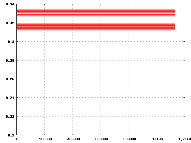
Running this class with $n=1\times 10^{6}$, the size of the output file was about 10 MB. To estimate the running time, we generate a graphic with the pairs $(k_{i},t_{i})$; see figure 2.

Figure 1: Pairs ($k_{i}$,$t_{i}$), where $t_{i}$ is the running time (seconds) between the computation of $\mu(k_{i-1})$ and $\mu(k_{i})$, using the class Beurling.

Figure 2: Pairs ($k_{i}$,$T_{i}$), where $T_{i}$ is the total running time (seconds) for the computation of $\mu(k_{i})$, using the Java class Beurling.

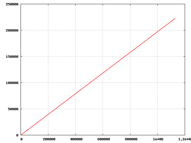
This graphic seems to suggest that square-free numbers can be divided in classes, and for each of these classes, the running time starting from the previous iteration $t_{i}$ is constant. We verify that all the square-free numbers in the range analyzed are generated by the program, and satisfy the condition $k_{i+1}<2k_{i}$, for $i\geqslant 2$. To estimate the total running time $T_{i}$ to compute $\mu(k_{i})$, we use the formula $T_{i}=\sum_{k=1}^{i}t_{k}$. The graphic with the pairs $(k_{i},T_{i})$ is shown in figure 2.

The program produced also four square-full, i.e. non square-free, numbers, shown in the table 1. All these square-full numbers $k_{i}$ satisfy $b_{i}(k_{i+1})-b_{i}(k_{i})=\mu(k_{i})=0$. However, as already stated, by the definition of the algorithm in section 4, it must be $b_{i}(k_{i+1})-b_{i}(k_{i})\neq 0$ for any generated number. Therefore, we strongly believe that the square-full numbers are generated purely by rounding errors.

Number $k$	$\mu(k)$	Divisible by
440375	0	$5^{2}$
551208	0	$2^{2}$
799460	0	$2^{2}$
979275	0	$5^{2}$

Table 1: The four square-full numbers produced by the class Beurling, with $n=1\times 10^{6}$.

7.2 The class BeurlingArrayList

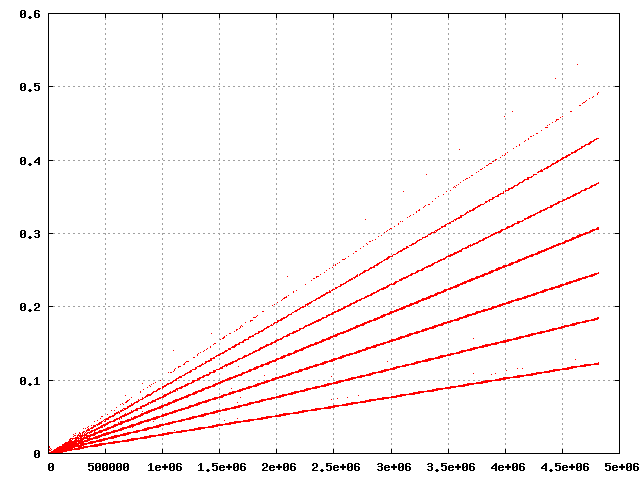
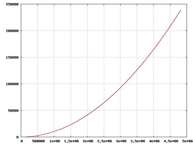
This class works as the previous one, but the computed values are stored in an array with dynamic size. We use this class to process $n=5\times 10^{6}$ numbers, using a relatively modest desktop machine. The graphics with the pairs $(k_{i},t_{i})$ and $(k_{i},T_{i})$ are shown in figures 4 and 4, respectively.

Figure 3: Pairs ($k_{i}$,$t_{i}$), where $t_{i}$ is the running time (seconds) between the computation of $\mu(k_{i-1})$ and $\mu(k_{i})$, using the class BeurlingArrayList.

Figure 4: Pairs ($k_{i}$,$T_{i}$), where $T_{i}$ is the total running time (seconds) for the computation of $\mu(k_{i})$, using the class BeurlingArrayList.

As in the case of figure 2, the square-free numbers $k_{i}$ seems to be divided in classes. However, in this case, the running time between two successive iterations $t_{i}$ grows linearly with $k_{i}$. All the square-free numbers in the range analyzed are generated by the program, and satisfy the condition $k_{i+1}<2k_{i}$, for $i\geqslant 2$. In the range analized, twenty square-full numbers were also generated by this class, probably by rounding errors, as explained above.

8 Concluding Remarks

In section 4 we define an algorithm that iteratively produces a sequence of numbers $k_{i}$ and functions $b_{i}$. The lemma 3 states a set of properties of these sequences suggesting that

• The numbers $k_{i}$ generated by the algorithm are square-free.

• The set of all the square-free numbers can be generated by the algorithm.

• The value of the Möbius function $\mu(k_{i})$ can be evaluated as $\mu(k_{i})=b_{i}(k_{i+1})-b_{i}(k_{i})$.

In section 5 we prove the logical equivalence of these properties. Unfortunately, using the definition of the algorithm, we cannot prove, neither disprove, if one of these conditions are satisfied. Note also that in order to determine $\mu(k_{i})$, it is necessary to generate the whole sequence $k_{1},k_{2},\dots,k_{i}$.

Numerical evidence seems to support the conjectures quoted above. However, this evidence is limited, and certainly not conclusive.

Fernando Auil

Escola de Artes, Ciências e Humanidades
Universidade de São Paulo
Arlindo Bettio 1000
CEP 03828-000
São Paulo - SP
Brasil

E-mail: auil@usp.br

References

- [1] T. M. Apostol, Introduction to Analytic Number Theory, Springer-Verlag, New York, 1976.
- [2] W. F. Donoghue, Distributions and Fourier Transforms, Academic Press, New York, 1969.
- [3] L. Báez-Duarte, Arithmetical Aspects of Beurling’s Real Variable Reformulation of the Riemann Hypothesis. arXiv:math/0011254v1 [math.NT]. Available in http://arxiv.org/abs/math/0011254v1.
- [4] L. Báez-Duarte, A Strengthening of the Nyman-Beurling Criterion for the Riemann Hypothesis. Atti Acad. Naz. Lincei 14 (2003) 5-11. arXiv:math/0202141v2 [math.NT]. Available in http://arxiv.org/abs/math/0202141v2.
- [5] B. Bagchi, On Nyman, Beurling and Baez-Duarte’s reformulation of the Riemann hypothesis, Proc. Indian Acad. Sci. (Math. Sci) 116 No. 2 (2003) 137-146.
- [6] H. M. Edwards, Riemann’s Zeta Function, Academic Press, New York, 1974.
- [7] G. H. Hardy, E. M. Wright. An Introduction to the Theory of Numbers, Oxford University Press, 5th ed., 1980.
- [8] E. C. Titchmarsh, The theory of the Riemann zeta function, Oxford Univ. Press, Oxford, 1951.