Optimal low-dispersion low-dissipation LBM schemes for computational aeroacoustics

Abstract

Lattice Boltmzmann Methods (LBM) have been proved to be very effective methods for computational aeroacoustics (CAA), which have been used to capture the dynamics of weak acoustic fluctuations. In this paper, we propose a strategy to reduce the dispersive and disspative errors of the two-dimensional (2D) multi-relaxation-time lattice Boltzmann method (MRT-LBM). By presenting an effective algorithm, we obtain a uniform form of the linearized Navier-Stokes equations corresponding to the MRT-LBM in wave-number space. Using the matrix perturbation theory and the equivalent modified equation approach for finite difference methods, we propose a class of minimization problems to optimize the free-parameters in the MRT-LBM. We obtain this way a dispersion-relation-preserving LBM (DRP-LBM) to circumvent the minimized dispersion error of the MRT-LBM. The dissipation relation precision is also improved. And the stability of the MRT-LBM with the small bulk viscosity is guaranteed. Von Neuman analysis of the linearized MRT-LBM is performed to validate the optimized dispersion/dissipation relations considering monochromatic wave solutions. Meanwhile, dispersion and dissipation errors of the optimized MRT-LBM are quantitatively compared with the original MRT-LBM . Finally, some numerical simulations are carried out to assess the new optimized MRT-LBM schemes.

1 Introduction

The lattice Boltzmann method (LBM) has emerged as a very effective methodology for the computational modeling of a wide variety of complex fluid flows [1]. Recent researches dealing with dispersion and dissipation relations of the LBM have shown that the LBM possesses the required accuracy to capture weak acoustic pressure fluctuations [2, 3, 4, 5]. The analysis indicated that the simple LBS possess lower numerical dissipation than the aeroacoustic optimized schemes of high-order schemes for Navier-Stokes equations [3]. The second-order accurate LBM has better dispersion capabilities than the classical Navier-Stokes schemes with 2nd-order accuracy in space and 3-step Runge-Kutta in time [3]. However, the dispersion error in the LBM is higher than that in the finite difference method with 3rd order spatial discretization and the 4th order time discretization, and also higher than that in dispersion relation preserving (DRP) 6th order accurate schemes. From the view of the numerical computations, for a given dispersion error, the LBM is faster than the high-order schemes for Navier-Stokes equations [3]. It has been shown that the dispersion error can be considered as a weakness of the LBM. For the classical lattice Boltzmann model (BGK-LBM), it is impossible to reduce the dispersion/dissipation errors. Meanwhile, it is reported that the original MRT-LBM [6, 7] and the BGK-LBM have exactly the same dispersion error and there exists a high dissipation of the acoustic modes for the MRT-LBM [3]. Here, the original MRT-LBM means we use the relaxation parameters recommended by Lallemand and Luo [6]. Furthermore, because of a high value of the bulk viscosity, the original MRT-LBM has a better stability compared with the BGK-LBM [3]. So, if the dissipation error of the MRT-LBM can be reduced and the stability can be guaranteed, it will be a good choice to simulate the acoustic problems using the MRT-LBM. The MRT-LBM can be optimized thanks to the existence of free parameters. By means of a Taylor series expansion [8, 9], it is easy to establish the relation between the linearized MRT-LBM (L-MRT-LBM) and the linearized Navier-Stokes equations (L-NSE) with the high-order truncation. The relations between the L-MRT-LBM and the L-NSE offer us a way to detect the influence of free parameters on the dispersion/dissipation relations. In the limit of linear acoustic, von Neumann analysis is a reliable tool to recover the dispersion and dissipation relations of the LBS. It is noted that this famous analysis method has been revisited and extended [3, 10]. Considering plane wave solutions, the relation between the wave-number $\bf{k}$ and the wave pulsation $\omega$ is described numerically. Then, the influence of free parameters on acoustic modes and shear modes will be analyzed. We propose a class of optimization strategies to minimize the dispersion/dissipation errors based on the matrix perturbation theory and the modified equation approach, leading to the definition of dispersion/dissipation-relation-preserving MRT-LBM (D2RP-LBM) schemes.

The basic idea of the DRP-LBM is significantly different from the idea of the classical DRP-schemes corresponding to finite difference schemes [11]. The classical DRP-schemes were established considering the finite difference approximation of the first derivative $\partial f/\partial x$ at the node of an uniform grid in wave-number space [11]. The classical DRP finite difference approximation of the first derivative $\partial f/\partial x$ in wave-number space is given by

$$\mathrm{i}\alpha\simeq\left(\frac{1}{\Delta x}\sum_{j=-N}^{M}a_{j}e^{\mathrm{i}\alpha j\Delta x}\right)\widetilde{f}.$$ (1)

The effective wave-number of Eq. (1) can be rewritten as follows

$$\widetilde{\alpha}=\frac{-\mathrm{i}}{\Delta x}\sum_{j=-N}^{M}a_{j}e^{\mathrm{i}\alpha j\Delta x}.$$ (2)

In the physical spaces, the expression of Eq. (1) is given as follows

$$\frac{\partial f}{\partial x}(x)\simeq\frac{1}{\Delta x}\sum_{j=-N}^{M}a_{j}f(x+j\Delta x).$$ (3)

In order to minimize the dispersion error, the following integral error $E$ is defined [11]

$$E=\int_{-\pi/2}^{\pi/2}|\alpha\Delta x-\widetilde{\alpha}\Delta x|^{2}d(\alpha\Delta x).$$ (4)

The classical DRP schemes only focus on proposing a best approximation of the first-derivative $\partial f/\partial x$ on an uniform mesh. In this paper, the proposed method to minimize the dispersion/dissipation error focus on obtaining a best global approximation of the exact L-NSE systems based on the recovered L-NSE by the L-MRT-LBM in wave-number spaces. Consequently, the resulting approximation addresses the best approaching relation between the exact L-NSE and the recovered L-NSE, but does not address individual derivatives. Formally, the research in this paper is dedicated to establishing the approximation between the following equation systems in wave-number spaces

$$\partial_{t}W=B\cdot W\ (\mbox{exact L-NSE}),\ \partial_{t}W=B_{,n}\cdot W+O(\delta t^{n})\ (\mbox{recovered L-NSE}),$$ (5)

where the square matrices $B$ and $B_{,n}$ are functions of wave-number vector $\mathbf{k}$, where $B_{,n}$ can be regarded as a perturbation of $B$. The vector $W$ denotes the perturbed macroscopic fluid flow quantities (density, momentum) in the linearized-NSE systems. In the paper, in order to reduce the dispersion error of the MRT-LBM for zero-mean flow, the truncation error is up to $O(\delta t^{5})$. Meanwhile, in order to reduce the dissipation error of the MRT-LBM for uniform flows, the truncation error is up to $O(\delta t^{4})$.

Furthermore, the proposed derivation of higher-order Taylor expansions of the MRT-LBM is very lengthy and complicated [8]. However, this derivation still pave a new way for establishing the relation between the L-MRT-LBM and the L-NSE. In order to avoid using this complex derivation, a new more effective and easy-to-use recursive algorithm is proposed to recover the L-NSE by the L-MRT-LBM. This recursive algorithm is established in wavenumber space. By this algorithm, the corresponding linearized macroscopic equations are expressed by an easy-to-handle matrix form. The optimization strategy is precisely built on the basis of this matrix equation. Finally, von Neumann analysis and numerical tests are implemented to assess the optimized MRT-LBM.

In next section, the methodology used to establish the transformation relation from the L-MRT-LBM to the L-NSE is given. The optimization strategies corresponding to the matrix equation are studied in Section 3. In Section 4, by von Neumann analysis, the DRP-LBM schemes are analyzed in spectral spaces. In the last section, the optimized MRT-LBM schemes are validated by benchmark problems.

2 Methodology for bridging from the MRT-LBM to the linearized Navier-Stokes equations

In this section, the basic theory of lattice Boltzmann schemes briefly reminded. Then, the linearized LBM is introduced and a method to establish the relation between the linearized LBS and the L-NSE is proposed.

2.1 Lattice Boltzmann schemes

The evolution equations of distribution functions of the basic lattice Boltzmann schemes are written as follows

$$f_{i}(x+v_{i}\delta t,t+\delta t)=f_{i}(x,t)+\Lambda_{ij}\left(f_{j}^{\rm(eq)}(x,t)-f_{j}(x,t)\right),\quad 0\leq i,j\leq N,$$ (6)

where $v_{i}$ belongs to the discrete velocity set $\mathcal{V}$, $f_{i}(x,t)$ is the discrete single particle distribution function corresponding to $v_{i}$ and $f_{i}^{\rm(eq)}$ denotes the discrete single particle equilibrium distribution function. $\delta t$ denotes the time step and $N+1$ is the number of discrete velocities. $\Lambda_{ij}$ is the relation matrix. From here, the repeated index indicates the Einstein summation for 0 to N except for the special indications. Let $\mathcal{L}\in\mathbb{R}^{d}$ ($d$ denotes the spatial dimension) denote the lattice system, the following condition is required [8]

$$x+v_{j}\delta t\in\mathcal{L},$$ (7)

that is to say, if $x$ is a node of the lattice, $x+v_{j}\delta t$ is necessarily another node of the lattice.

For the BGK-LBM, the relaxation matrix is set as follows

$$\Lambda_{ij}=s\delta_{ij},$$ (8)

where $s$ is related to the relaxation frequency of the BGK-LBM.

The standard MRT-LBM has the following form [8, 6]

$$m_{i}=W_{i}=m_{i}^{\rm(eq)},0\leq i\leq d,$$ (9)

and

$$m_{i}(x+\delta tv_{j},t+\delta t)=m_{i}(x,t)+s_{i}\left(m_{i}^{\rm(eq)}(x,t)-m_{i}(x,t)\right),d+1\leq i\leq N,$$ (10)

where the index $i$ doesn’t indicate the summation. According to the work of Lallemand and Luo [6], the relaxation parameters in Eq. (10) must satisfy the following stability constrain

$$s_{i}\in(0,2),d+1\leq i\leq N.$$ (11)

The relaxation matrix $\Lambda$ associated with Eqs. (9) and (10) is defined by

$$\Lambda=M^{-1}SM,$$ (12)

where $S$ is a diagonal matrix which is related to the relaxation parameters of the MRT-LBM. $M=\left(M_{ij}\right)_{0\leq i\leq N,0\leq i\leq N}$ is the transformation matrix, which satisfies the following basic conditions [6]

$$M_{0j}=1,M_{\alpha j}=v_{j}^{\alpha},(1\leq\alpha\leq d).$$ (13)

The macroscopic quantities are defined by [6, 8]

$$m_{i}=M_{ij}f_{j},\quad m_{i}^{\rm(eq)}=M_{ij}f_{j}^{\rm(eq)}.$$ (14)

2.2 The Linearized MRT-LBM and the higher-order linearized NSE

The equilibrium function $m_{i}^{\rm(eq)}$ ($d+1\leq i\leq N$) is the function of conservative quantities $W_{i}$ ($W_{i}=m_{i}^{\rm(eq)},0\leq i\leq d$) (we use the same notations as Dubois and Lallemand [8])

$$m_{i}^{\rm(eq)}=G_{i}\left(\{W_{j}\}_{0\leq j\leq d}\right),d+1\leq i\leq N.$$ (15)

or

$$m_{i}^{\rm(eq)}=G_{i}\left(\{W_{j}\}_{0\leq j\leq d}\right)=G_{ij}W_{j}=G_{ij}m_{j}$$ (16)

In order to implement the linear stability analysis and recover the linearized macroscopic equations, we introduce the linearized form of Eq. (15) around reference states [3, 8, 6]. Using Eq. (16), the linearized description of Eqs. (9) and (10) can be written as follows

$$m_{i}(x,t+\delta t)=M_{il}M_{lp}^{-1}\Psi_{pr}m_{r}(x-v_{l}\delta t,t),$$ (17)

where the matrix $\Psi$ has the following form

$$\Psi=\left(\begin{array}[]{cc}\left(\mathrm{I}_{ij}\right)_{0\leq i\leq d,0\leq j\leq d}&0\\ \Theta&\left(\mathrm{I}_{ij}-S_{ij}\right)_{d+1\leq i\leq N,d+1\leq j\leq N}\end{array}\right)$$ (18)

where $\Theta_{ij}=s_{i}G_{ij}$. A is matrix with the size $(N-d-1)\times(d+1)$), $\mathrm{I}$ is an identity matrix and the diagonal matrix $S$ is defined by

$$S={\rm Diag}(\underbrace{0,\ldots,0}_{d+1},\underbrace{s_{d+1},\ldots,s_{N}}_{N-d-1}.$$ (19)

In Eq. (17), the indices $l$, $p$ and $r$ indicate the summations from 0 to N.

In order to derive the linearized high-order equations, one assumes that the discrete single particle distribution $f_{i}$ belongs to $C^{\infty}(T\times\mathcal{L})$ (a functional set, in which the element possesses a sufficiently smooth property with respect to the time domain $T$ and spatial domain $\mathcal{L}$ ). This assumption is also used by Junk et. al. for asymptotic analysis of the LBM [12]. This regularity hypothesis indicates that macroscopic quantities $m_{i}$ are smooth ones and that the linearized system (17) is well defined.

The next step consists of performing the Taylor series expansion of the right hand of Eq. (17), yielding

$$m_{i}(x,t+\delta t)=\sum_{n=0}^{\infty}\frac{\delta t^{n}}{n!}M_{il}(-v_{l}^{\alpha}\partial_{\alpha})^{n}M^{-1}_{lp}\Psi_{pr}m_{r},$$ (20)

where $\alpha$ indicates the summation from $1$ to $d$.

Now, we define the matrix $A^{*}_{,n}=\left(A^{*}_{ij,n}\right)_{0\leq i\leq N,0\leq j\leq N}$ as follows

$$A^{*}_{ir,n}=\frac{1}{n!}M_{il}(-v_{l}^{\alpha}\partial_{\alpha})^{n}M_{lp}^{-1}\Psi_{pr}.$$ (21)

When we need to derive equivalent equations or modified equations, it is difficult to use the matrix $A^{*}_{,n}$ to carry out the calculations. In order to overcome this difficulty, we use the differential operators in spectral space. Let us note $\partial_{\alpha}=\mathrm{i}k_{\alpha}$, with $k_{\alpha}$ the wave-number in the $\alpha$ -direction and $\mathrm{i}^{2}=-1$. Then, in spectral space, the matrix $A^{*}_{,n}$ has the following form ($A_{,n}=(A_{ij,n})_{0\leq i\leq N,0\leq j\leq N}$)

$$A_{ir,n}=\frac{1}{n!}M_{il}(-\mathrm{i}v_{l}^{\alpha}k_{\alpha})^{n}M_{lp}^{-1}\Psi_{pr}.$$ (22)

Therefore, Eq. (20) can be rewritten as follows

$$m_{i}(x,t+\delta t)=\sum_{n=0}^{J-1}\delta t^{n}A_{ir,n}m_{r}+O(\delta t^{J}).$$ (23)

In order to derive the L-NSE corresponding to the L-MRT-LBM defined by Eq. (23), we introduce an original recursive algorithm. Given $m_{i}=W_{i}(0\leq i\leq d)$ (macroscopic conservative quantities), the algorithm is given as follows

• Initial step. The initial $\Phi_{,1}$ and $B_{,1}$ are given as follows

  $$\Phi_{ij,1}=\delta_{ij}(0\leq i\leq d),\Phi_{ij,1}=\frac{1}{s_{i}}\Psi_{ij}(d+1\leq i\leq N),$$ (24)

  $$B_{ij,1}=A_{ir,1}\Phi_{rj,1}.$$ (25)

  Let $W=\{W_{i}\}_{0\leq i\leq d}$ and $m=\{m_{i}\}_{0\leq i\leq N}$ denote the vector of the conservative quantities and the vector of all macroscopic quantities respectively.

  At the first order of $\delta t$, for all macroscopic quantities, we have

  $$m_{i}=\Phi_{ij,1}W_{j}+O(\delta t),0\leq i\leq N.$$ (26)

  By the matrix form, we have

  $$m=\Phi_{,1}W+O(\delta t).$$ (27)

  At the first-order of $\delta t$, for conservative quantities, we have

  $$\partial_{t}W_{i}=A_{ir,1}\Phi_{rj,1}W_{j}+O(\delta t).$$ (28)

  The matrix form is

  $$\partial_{t}W=A_{,1}\Phi_{,1}W_{j}+O(\delta t).$$ (29)

• Recursive formula for all macroscopic quantities. $\Phi_{ij,n}$ can be given as follows

  $$\Phi_{ij,n}=\frac{1}{s_{i}}(\Psi_{ij}-\sum_{l=1}^{n-1}\frac{\delta t^{l}}{l!}\Phi_{ir,n-l}B_{rj,n-l}^{l}+\sum_{l=1}^{n-1}\delta t^{l}A_{ir,l}\Phi_{rj,n-l}),d+1\leq i\leq N$$ (30)

  and

  $$\Phi_{ij,n}=\delta_{ij},(0\leq i\leq d).$$ (31)

  Eliminating the higher-order term of $\delta t^{n-1}$, we have

  $$\Phi_{ij,n}=\sum_{l=0}^{n-1}\delta t^{l}{\rm Coeff}(\Phi_{ij,n},\delta t,l),$$ (32)

  where ${\rm Coeff(\cdot,\cdot,\cdot)}$ is a function which extracts the coefficients of the polynomials, for example, $f(x)=\sum_{i=0}^{n}a_{i}x^{i}$

  $${\rm Coeff}(f(x),x,i)=a_{i}.$$ (33)

  According to Eqs.(30) and (32), we have

  $$m=\Phi_{,n}W+O(\delta t^{n}).$$ (34)

• Recursive formula for conservative quantities. $B_{ij,n}$ is presented as follows

  $$B_{ij,n}=-\sum_{l=1}^{n-1}\frac{\delta t^{l}}{(l+1)!}B_{ij,n-l}^{l+1}+\sum_{l=1}^{n}\delta t^{l-1}A_{ir,l}\Phi_{rj,n+1-l}.$$ (35)

  Eliminating the higher-order term of $\delta t^{n-1}$, we have

  $$B_{ij,n}=\sum_{l=0}^{n-1}\delta t^{l}{\rm Coeff}(B_{ij,n},\delta t,l).$$ (36)

  Now, for the conservative quantities, we have the following equation system

  $$\partial_{t}W=B_{,n}\cdot W+O(\delta t^{n}).$$ (37)

  Using Eqs. (32), (34), (36) and (37), we can get the coefficient matrix of the conservative quantities at any order of $\delta t$ . Details are displayed in A.

2.3 Illustrating example: application to a 2D MRT-LBM

In this section, we illustrate the algorithm presented in 2.2 considering a 2D MRT-LBM. For the standard 2D MRT-LBM, the equilibrium distribution functions are described as follow [6, 13]

$$m^{\rm(eq)}=\left\{\rho,j_{x},j_{y},-2\rho+\frac{3}{\rho}(j_{x}^{2}+j_{y}^{2}),\rho-\frac{3}{\rho}(j_{x}^{2}+j_{y}^{2}),-j_{x},-j_{y},\frac{1}{\rho}(j_{x}^{2}-j_{y}^{2}),\frac{1}{\rho}j_{x}j_{y}\right\},$$ (38)

where $j_{x}$ and $j_{y}$ denote the x-momentum and y-momentum respectively, and $\rho$ represents the density ($W_{0}=m_{0}=\rho,W_{1}=m_{1}=j_{x},W_{2}=m_{2}=j_{y}$). The corresponding matrix $\Psi$ is given by

$$\Psi=\left[\begin{array}[]{ccccccccc}1&0&0&0&0&0&0&0&0\\ 0&1&0&0&0&0&0&0&0\\ 0&0&1&0&0&0&0&0&0\\ -2s_{e}-3(U^{2}+V^{2})s_{e}&6Us_{e}&6Vs_{e}&1-s_{e}&0&0&0&0&0\\ s_{\epsilon}+3(U^{2}+V^{2})s_{\epsilon}&-6Us_{\epsilon}&-6Vs_{\epsilon}&0&1-s_{\epsilon}&0&0&0&0\\ 0&-s_{q}&0&0&0&1-s_{q}&0&0&0\\ 0&0&-s_{q}&0&0&0&1-s_{q}&0&0\\ -(U^{2}-V^{2})s_{\nu}&2Us_{\nu}&-2Vs_{\nu}&0&0&0&0&1-s_{\nu}&0\\ -UVs_{\nu}&Vs_{\nu}&Us_{\nu}&0&0&0&0&0&1-s_{\nu}\end{array}\right]$$ (39)

The diagonal elements of the corresponding diagonal matrix $S$ are set as follows

$$s_{0}=s_{1}=s_{2}=0,s_{3}=s_{e},s_{4}=s_{\epsilon},s_{5}=s_{6}=s_{q},s_{7}=s_{8}=s_{\nu}.$$ (40)

For the original MRT-LBM [6], only $s_{\nu}$ is a free parameter, and $s_{e}=1.64$, $s_{\epsilon}=1.54$, $s_{q}=1.9$. The analogous form of $\Psi$ can be found in existing literature [6, 8, 13]. However, there still exist some slight differences. The derivation of $\Psi$ can be achieved by means of the first-order Taylor series expansion with respect to $\rho$, $j_{x}$ and $j_{y}$ at reference states. In the expression of $\Psi$, $(U,V)$ to denote the uniform flow velocity components.

For the sake of convenience, we introduce the following relation

$$\sigma_{\eta}=\frac{1}{s_{\eta}}-\frac{1}{2},$$ (41)

where $\eta$ stands for any notations in the set $\{e,\epsilon,q,\nu\}$.

2.3.1 Considering the zero-mean flows $(U,V)=(0,0)$

Now, when the truncated error term is equal to $O(\delta t^{5})$ , the coefficient matrix $B_{,5}$ with the zero-mean flow can be described by the summation of five matrices. The first two matrices are given as follows, which describe the specific terms in the Navier-Stokes equations.

The coefficient matrix associated with $\delta t^{0}$ is

$$\mathrm{i}\cdot\left[\begin{array}[]{ccc}0&-{\it k_{x}}&-{\it k_{y}}\\ \vskip 6.0pt plus 2.0pt minus 2.0pt\cr-\frac{1}{3}\,{\it k_{x}}&0&0\\ \vskip 6.0pt plus 2.0pt minus 2.0pt\cr-\frac{1}{3}\,{\it k_{y}}&0&0\end{array}\right]$$ (42)

The coefficient matrix associated with $\delta t$ is given by

$$\left[\begin{array}[]{ccc}0&0&0\\ \vskip 6.0pt plus 2.0pt minus 2.0pt\cr 0&-\frac{1}{3}\,{{\it k_{x}}}^{2}\sigma_{e}-\frac{1}{3}\,{{\it k_{x}}}^{2}\sigma_{\nu}-\frac{1}{3}\,{{\it k_{y}}}^{2}\sigma_{\nu}&-\frac{1}{3}\,{\it k_{x}}\,{\it k_{y}}\,\sigma_{e}\\ \vskip 6.0pt plus 2.0pt minus 2.0pt\cr 0&-\frac{1}{3}\,{\it k_{x}}\,{\it k_{y}}\,\sigma_{e}&-\frac{1}{3}\,{{\it k_{x}}}^{2}\sigma_{\nu}-\frac{1}{3}\,{{\it k_{y}}}^{2}\sigma_{e}-\frac{1}{3}\,{{\it k_{y}}}^{2}\sigma_{\nu}\end{array}\right]$$ (43)

At the higher-order truncated errors of $\delta t$, the coefficient matrices are given in B. Compared with the results given by Dubois and Lallemand [8], it is shown that the proposed algorithm yields the correct results. Meanwhile, the higher-order terms of $\delta t$ are offered by our algorithm explicitly.

2.3.2 Considering the uniform flow $(U,V)$ $(U\neq 0$ or $V\neq 0)$

When the truncated error term is equal to $O(\delta t^{2})$ , the coefficient matrix $B_{,2}$ with the uniform flow can be described by the summation of two matrices. The coefficient matrix associated with $\delta t^{0}$ is

$$\mathrm{i}\cdot\left[\begin{array}[]{ccc}0&-{k_{x}}&-{k_{y}}\\ \vskip 6.0pt plus 2.0pt minus 2.0pt\cr-\frac{1}{3}\,{k_{x}}+{k_{x}}\,{U}^{2}+{k_{y}}\,UV&-2\,{k_{x}}\,U-{k_{y}}\,V&-{k_{y}}\,U\\ \vskip 6.0pt plus 2.0pt minus 2.0pt\cr-\frac{1}{3}\,{k_{y}}+{k_{y}}\,{V}^{2}+{k_{x}}\,UV&-{k_{x}}\,V&-2\,{k_{y}}\,V-{k_{x}}\,U\end{array}\right]$$ (44)

The coefficients of $\delta t$ are given in C.

From the coefficient matrix, it is clear that the correct convection terms of the L-NSE can be given by the L-MRT-LBM. However, the correct dissipation coefficients can not be obtained by the L-MRT-LBM with respect to the uniform flow, yielding the definition of a flow-dependent viscosity. Furthermore, this dependence also becomes a source of the non-Galilean invariance.

From 2.3.1 and 2.3.2, it is known at the zeroth-order and the first-order of $\delta t$, the relaxation parameters $s_{\epsilon}$ and $s_{q}$ have no influence on the recovered L-NSE. Here, the given form of the L-NSE is generated with respect to the small perturbations of the density $\rho$ and the momentum quantities $(j_{x},j_{y})$.

3 Optimization strategies of free parameters in the MRT-LBM

In this section, the original optimization strategies of free parameters in the MRT-LBM are proposed based on the matrix perturbation theory and the modified equations. The optimized parameters will be determined in order to obtain the optimal dispersion/dissipation relations.

3.1 The matrix perturbation theory for the L-NSE corresponding to the L-MRT-LBM

From Eq. (37), it is known that the dispersion and dissipation relations of the L-MRT-LBM are determined by the matrix $B_{,n}\in C^{(1+d)\times(1+d)}$, where $C^{(1+d)\times(1+d)}$ denotes the $(1+d)\times(1+d)$ complex matrix set, if the truncation error is developed up to the $n$th-order of $\delta t$. Here, $B$ refers to the coefficient matrix of the exact L-NSE in wave-number space similar to the matrix $B_{,n}$ in Eq. (37). This means that for the exact L-NSE, one has the following expression

$$\partial_{t}W=B\cdot W.$$ (45)

For a given $n$, if the errors terms with order higher that $\delta t^{n}$ are neglected, the main deviation of dispersion and dissipation relations between the L-MRT-LBM and the L-NSE originates in the differences between eigenvalues of $B_{,n}$ and those of $B$.

Now, we introduce the perturbation matrix $M_{\varepsilon}\in C^{(1+d)\times(1+d)}$ defined as

$$B_{,n}=B+M_{\varepsilon}.$$ (46)

Let $B$ have eigenvalues $\lambda_{1},\ldots,\lambda_{n}$ and $B_{,n}$ have eigenvalues $\tilde{\lambda}_{1},\ldots,\tilde{\lambda}_{n}$. The spectral variation of $B_{,n}$ with respect to $B$ is [14]

$${\rm SV}_{B}(B_{,n})\equiv\max_{i}\min_{j}|\tilde{\lambda}_{i}-\lambda_{j}|.$$ (47)

Then [14],

$${\rm SV}_{B}(B_{,n})\leq(\|B\|_{2}+\|B_{,n}\|_{2})^{1-1/(d+1)}\|M_{\varepsilon}\|_{2}^{1/(d+1)},$$ (48)

where $\|\cdot\|_{2}$ is the spectral norm of matrices. For all $A\in C^{(d+1)\times(d+1)}$, $\|\cdot\|_{2}$ is defined by

$$\|A\|_{2}=\sqrt{\lambda_{\max}(A^{H}A)}=\sigma_{\max}(A),$$ (49)

where $A^{H}$ denotes the conjugate transpose of $A$. $\lambda_{\max}(A^{H}A)$ is the largest eigenvalue of $A^{H}A$ and $\sigma_{\max}(A)$ is the largest singular value of $A$. In order to establish the direct relation between elements and eigenvalues of matrices explicitly, the Frobenius norm is given as follows for any $A=(a_{ij})_{0\leq i\leq d,0\leq j<j}\in C^{(d+1)\times(d+1)}$ [15],

$$\|A\|_{F}=\sqrt{\sum_{i=0}^{d}\sum_{j=0}^{d}|a_{ij}|^{2}}=\sqrt{{\rm trace}(A^{H}A)}=\sqrt{\sum_{i=0}^{d}\sigma_{i}^{2}},$$ (50)

where $\sigma_{i}$ denotes the singular values of $A$.

Furthermore, let $\sigma(B)=\{\lambda_{0},\ldots,\lambda_{d+1}\}$, the multiset of $B$’s eigenvalues, and set

$$\Lambda={\rm diag}(\lambda_{0},\ldots,\lambda_{d+1}),\Lambda_{\tau}={\rm diag}(\lambda_{\tau(0)},\ldots,\lambda_{\tau(d+1)}),$$ (51)

where $\tau$ is a permutation of $\{1,\ldots,d+1\}$. Let $\sigma(B_{,n})=\{\tilde{\lambda}_{0},\ldots,\tilde{\lambda}_{d+1}\}$, the multiset of $B_{,n}$’s eigenvalues, and set

$$\tilde{\Lambda}={\rm diag}(\tilde{\lambda}_{0},\ldots,\tilde{\lambda}_{d+1}),\tilde{\Lambda}_{\tau}={\rm diag}(\tilde{\lambda}_{\tau(0)},\ldots,\tilde{\lambda}_{\tau(d+1)}),$$ (52)

Then, there exists a permutation $\tau$ such that the following inequality is satisfied [14, 16]

$$\|\Lambda-\tilde{\Lambda}_{\tau}\|_{2}\leq 2\left\lfloor\frac{d+1}{2}\right\rfloor(\|B\|_{2}+\|B_{,n}\|_{2})^{1-1/(d+1)}\|M_{\varepsilon}\|_{2}^{1/(d+1)}.$$ (53)

Since $\|M_{\varepsilon}\|_{2}\leq\|M_{\varepsilon}\|_{F}$, the minimization of ${\rm SV}_{B}(B_{,n})$ or $\|\Lambda-\tilde{\Lambda}_{\tau}\|_{2}$ means $\|M_{\varepsilon}\|_{F}$ should be minimized to reduce both dispersion and dissipation errors associated with the MRT-LBM schemes.

3.2 Optimization methodology

The following wave-number definition in Eq.(37) is considered

$$k_{x}=k\cdot{\rm cos}(\theta),k_{y}=k\cdot{\rm sin}(\theta).$$ (54)

Substituting Eq. (54) into Eq. (37) and considering the uniform flow $(U,V)$, we can get the following formal expression for $B_{,n}$

$$B_{,n}=\sum_{l=0}^{n-1}\delta t^{l}k^{l+1}b_{ij,n}^{l}(\theta,\Xi,U,V),$$ (55)

where $b_{ij,n}^{l}$ is a function of $\theta$, $\Xi$ and $(U,V)$. $\Xi$ denotes the following set (about extra parameters, refer to the non-standard MRT-LBM [13])

$$\Xi=\{\alpha,\beta,\lambda,\sigma_{e},\sigma_{\epsilon},\sigma_{q},\sigma_{\nu}\}.$$ (56)

For the standard MRT-LBM, the parameters $\alpha$, $\beta$ and $\lambda$ are equal to 1, -3 and -2, respectively. In order to handle the influences of the uniform flows, we consider the following uniform flows

$$U=u_{m}\cdot{\rm cos}(\vartheta),V=u_{m}\cdot{\rm sin}(\vartheta),$$ (57)

where $u_{m}$ denotes the magnitude of the uniform velocity. Now, Eq. (55) has the following form

$$B_{,n}=\sum_{l=0}^{n-1}\delta t^{l}k^{l+1}b_{ij,n}^{l}(\theta,\vartheta,\Xi,u_{m}).$$ (58)

Furthermore, Eq. (58) is rewritten as follows

$$B_{ij,n}=\frac{1}{\delta t}\mathcal{B}_{ij,n}(\delta tk,\theta,\vartheta,\Xi,u_{m})=\frac{1}{\delta t}\sum_{l=1}^{n}(\delta tk)^{l}b_{ij,n}^{l-1}(\theta,\vartheta,\Xi,u_{m}).$$ (59)

For the L-NSE, there exists the similar matrix $\mathcal{B}$ defined by $\mathcal{B}=\delta tB$. It is known that for the MRT-LBM, the dispersion error corresponding to the L-MRT-LBM stems from the odd-order coefficient matrix $M_{\epsilon}^{O}$ of $\delta tk$ in $\mathcal{M}_{\epsilon}=\delta tM_{\varepsilon}=\mathcal{B}_{,n}-\mathcal{B}$, and the dissipation error comes from the even-order coefficient matrix $M_{\epsilon}^{E}$ of $\delta tk$ in $M_{\epsilon}$. So, the perturbation matrix $M_{\epsilon}$ can be expressed as follows

$$\mathcal{M}_{\epsilon}=M_{\epsilon}^{O}+M_{\epsilon}^{E}.$$ (60)

3.2.1 The zero-mean flow case

Considering $u_{m}=0$, then, $\mathcal{M}_{\epsilon}=\mathcal{B}_{,n}-\mathcal{B}$ is a function of $\delta tk,\theta$ and $\Xi$. According to Sec. 2.3.1,

$$\mathcal{M}_{\epsilon}=\sum_{l=3}^{n}(\delta tk)^{l}b_{ij,n}^{l-1}(\theta,\vartheta,\Xi,u_{m})=\sum_{l=3}^{n}(\delta tk)^{l}b_{ij,n}^{l-1}(\theta,\Xi),$$ (61)

$$M_{\epsilon}^{O}=\sum_{1\leq l\leq n,2l+1\leq n}(\delta tk)^{2l+1}b_{ij,n}^{2l}(\theta,\Xi),$$ (62)

$$M_{\epsilon}^{E}=\sum_{1\leq l\leq n,2l\leq n}(\delta tk)^{2l}b_{ij,n}^{2l-1}(\theta,\Xi).$$ (63)

According to the theory of the finite difference method (FDM) [17], Eq. (37) can be regarded as the modified equation of Eq. (45). In modified equations, the higher even-order derivatives beyond Eq. (45) cause numerical dissipation and the higher odd-order derivatives cause numerical dispersion [17].

In order to reduce the dispersion error, when $\sigma_{e}$ and $\sigma_{\nu}$ are specified, it is proposed here to minimize the following cost function:

$$F^{o}(\Xi)=\int_{0}^{\pi}\int_{0}^{2\pi}\|M_{\epsilon}^{O}\|_{F}^{2}{\rm d}\theta{\rm d}(\delta tk).$$ (64)

For the standard MRT-LBM, the parameters $\sigma_{\epsilon}$ and $\sigma_{q}$ need to be determined. The corresponding conditions are

$$\sigma_{\epsilon}\geq 0,\sigma_{q}\geq 0,$$ (65)

that is to say,

$$s_{\epsilon},s_{q}\in(0,2].$$ (66)

In order to separate the kinetic modes form the modes directly affecting hydrodynamic transport, Lallemand and Luo [6] suggested that $s_{\epsilon}$ and $s_{q}$ should be kept slightly larger than 1. Accordingly, it was implied that $s_{\epsilon},s_{q}\in(1,2)$. In this paper, $s_{\epsilon},s_{q}$ are taken in the range $(0,2]$.

Furthermore, the same method can be used to reduce dissipation error. The corresponding cost function is

$$F^{e}(\Xi)=\int_{0}^{\pi}\int_{0}^{2\pi}\|M_{\epsilon}^{E}\|_{F}^{2}{\rm d}\theta{\rm d}(\delta tk).$$ (67)

If both of dispersion and dissipation errors need to be reduced, according to Eqs. (48) and (53), minimizing error between hydrodynamic modes of the L-NSE and the L-MRT-LBM is achieved by minimizing

$$\mathcal{F}(\Xi)=\int_{0}^{\pi}\int_{0}^{2\pi}\|\mathcal{M}_{\epsilon}\|_{F}^{2}{\rm d}\theta{\rm d}(\delta tk)=\int_{0}^{\pi}\int_{0}^{2\pi}(\|M_{\epsilon}^{O}\|_{F}^{2}+\|M_{\epsilon}^{E}\|_{F}^{2}){\rm d}\theta{\rm d}(\delta tk).$$ (68)

3.2.2 The non-zero mean flow case

Considering $u_{m}\neq 0$, then, $\mathcal{M}_{\epsilon}=\mathcal{B}_{,n}-\mathcal{B}$ is a function of $\delta tk,\theta,\vartheta,\Xi$ and $u_{m}$. It is known that it is difficult for the non-zero mean flows to determine the values of free parameters locally, because the optimization problems must be solved at each lattice node. In order to avoid solving optimization problems locally, the minimization problems will be integrated with respect to $\vartheta$ and $u_{m}$. Here, it is necessary to mention that the similar relations of Eqs. (62) and (63) about $M_{\epsilon}^{E}$ and $M_{\epsilon}^{O}$ are not satisfied for the non-zero mean flows.

In order to minimize the dispersion error, the following cost function is introduced

$$G^{e}(\Xi)=\int_{0}^{u_{0}}\int_{0}^{2\pi}\int_{0}^{\pi}\int_{0}^{2\pi}\|M_{\epsilon}^{E}\|_{F}^{2}{\rm d}\theta{\rm d}(\delta tk){\rm d}\vartheta{\rm d}u_{m},$$ (69)

where $u_{0}$ is the upper bound of lattice velocity magnitude. Generally, $u_{0}$ is taken equal to 0.2. Similarly, in order to minimize the dissipation error, we have the cost function

$$G^{o}(\Xi)=\int_{0}^{u_{0}}\int_{0}^{2\pi}\int_{0}^{\pi}\int_{0}^{2\pi}\|M_{\epsilon}^{O}\|_{F}^{2}{\rm d}\theta{\rm d}(\delta tk){\rm d}\vartheta{\rm d}u_{m}.$$ (70)

For the non-zero mean flows, the optimization problem of minimizing error between hydrodynamic modes of the L-NSE and the L-MRT-LBM is associated with the following cost function

$$\mathcal{G}(\Xi)=\int_{0}^{u_{0}}\int_{0}^{2\pi}\int_{0}^{\pi}\int_{0}^{2\pi}\|\mathcal{M}_{\epsilon}\|_{F}^{2}{\rm d}\theta{\rm d}(\delta tk){\rm d}\vartheta{\rm d}u_{m}.$$ (71)

3.2.3 A non-zero mean flow case and separating the bulk-viscosity terms from the dissipation coefficient matrix

It is observed that when the shear viscosity is very small, the magnitude of the bulk viscosity is very sensitive to the stability numerically and theoretically. If the bulk viscosity is also too small, the MRT-LBM schemes will be unstable. Meanwhile, although we adopt the optimization strategy detailed in Sec. 3.2.2 and the optimized MRT-LBM appears to be more stable than the original MRT-LBM, the stability of the obtained MRT-LBM is still very sensitive. Furthermore, it is known that for linear acoustic problems, the values of shear and bulk viscosity are often very small and the dissipation effects from the shear and bulk viscosity can nearly be neglected. In the simulations, if the bulk viscosity is too large, the pressure fluctuations will be damped very significantly. This over-dissipative behavior should be avoided for aeroacoustic problems. In order to handle the low bulk viscosity problems, we propose a new optimization strategy. For the uniform flows, the linearized convection terms are given by the matrix (44) in spectral space, and the recovered linearized dissipation matrix is also given by a matrix in C. The exact linearized dissipation coefficient matrix with the uniform flows is given by (the simple derivations with respect to the perturbation of $\rho$, $j_{x}$ and $j_{y}$ are neglected)

$$\left[\begin{array}[]{ccc}0&0&0\\ \vskip 6.0pt plus 2.0pt minus 2.0pt\cr 0&-\frac{1}{3}\,{{\it k_{x}}}^{2}\sigma_{e}-\frac{1}{3}\,{{\it k_{x}}}^{2}\sigma_{\nu}-\frac{1}{3}\,{{\it k_{y}}}^{2}\sigma_{\nu}&-\frac{1}{3}\,{\it k_{x}}\,{\it k_{y}}\,\sigma_{e}\\ \vskip 6.0pt plus 2.0pt minus 2.0pt\cr 0&-\frac{1}{3}\,{\it k_{x}}\,{\it k_{y}}\,\sigma_{e}&-\frac{1}{3}\,{{\it k_{x}}}^{2}\sigma_{\nu}-\frac{1}{3}\,{{\it k_{y}}}^{2}\sigma_{e}-\frac{1}{3}\,{{\it k_{y}}}^{2}\sigma_{\nu}\end{array}\right]$$ (72)

It is clear that the coefficient matrix (72) has the same expression as the coefficient matrix (43). The coefficient matrix corresponding to bulk viscosity is given by

$$\mathscr{B}=\left[\begin{array}[]{ccc}0&0&0\\ \vskip 6.0pt plus 2.0pt minus 2.0pt\cr 0&-\frac{1}{3}\,{{\it k_{x}}}^{2}\sigma_{e}&-\frac{1}{3}\,{\it k_{x}}\,{\it k_{y}}\,\sigma_{e}\\ \vskip 6.0pt plus 2.0pt minus 2.0pt\cr 0&-\frac{1}{3}\,{\it k_{x}}\,{\it k_{y}}\,\sigma_{e}&-\frac{1}{3}\,{{\it k_{y}}}^{2}\sigma_{e}\end{array}\right]$$ (73)

The new perturbation matrix $\mathcal{M}_{\epsilon}$ is defined by $\mathcal{M}_{\epsilon}=\mathcal{B}_{,n}-\mathcal{B}+\mathscr{B}$. The matrix $\mathcal{M}_{\epsilon}$ possesses the information of the bulk viscosity at the first-order of $\delta t$. The optimization strategies are kept the same as those in Sec. 3.2.2. The parameter $\sigma_{e}$, which is related to the bulk viscosity, can be taken as an user-specified or free parameter for acoustic problems. If the MRT-LBM is considered as a high-precision solver for the nearly incompressible flows, $\sigma_{e}$ can be set as a free parameter.

4 von Neumann analysis of the dispersion and dissipation relations

In this part, the optimization strategies will be investigated by means of von Neumann analysis. At the same time, we will give some numerical results of the dispersion and dissipation relations.

4.1 Theoretical dispersion and dissipation relations for the L-MRT-LBM and the L-NSE

In order to apply von Neumann analysis to validate the optimized parameters, it is necessary to give the expressions of the L-MRT-LBM in frequency-wave number space. Considering a uniform mean part $f_{i}^{0}$ and a fluctuating part $f_{i}{{}^{\prime}}$, the equilibrium distribution function can be linearized as [3, 4]

$$f^{\rm(eq)}_{i}(\{f_{j}^{0}+f_{j}{{}^{\prime}}\}_{0\leq j\leq N})=f_{i}^{\rm(eq),0}+\left.\frac{\partial f^{\rm(eq)}_{i}}{\partial f_{j}}\right|_{f_{j}=f_{j}^{0}}\cdot f_{j}{{}^{\prime}}+O(f_{j}^{\prime 2}).$$ (74)

Then, considering a plane wave solution of the linearized equation

$$f_{j}^{\prime}=A_{j}{\rm exp}[\mathrm{i}({\bf k}\cdot{\bf x}-\omega t)],$$ (75)

according to Eqs. (74), (75) and (14), we get the following eigenvalue problem for the L-MRT-LBM in frequency-wave number space [3, 4, 6]

$$e^{-\mathrm{i}\omega}{\bf f}^{\prime}=M^{\rm mrt}{\bf f}^{\prime},$$ (76)

where the matrix $M^{\rm mrt}=A^{-1}\left[I-M^{-1}SMN^{\rm bgk}\right]$, and $N^{\rm bgk}$ is defined by

$$N^{\rm bgk}_{ij}=\delta_{ij}-\left.\frac{\partial f_{i}^{\rm(eq)}}{f_{j}}\right|_{f_{j}=f_{j}^{0}}.$$ (77)

For the L-NSE, the analytical acoustic modes $\omega^{\pm}$ and shear modes $\omega^{s}(\bf k)$ are given by [18]

$$\left\{\begin{array}[]{l}Re[\omega^{\pm}({\bf k})]=|{\bf k}|(\pm c_{s}({\bf k})+|{\bf u}|{\bf cos}(\widehat{\bf k\cdot u})),\\ Im[\omega^{\pm}({\bf k})]=-|{\bf k}|^{2}\frac{1}{2}\left(\frac{2d-2}{d}\nu({\bf k})+\eta(\bf k))\right),\\ Re[\omega^{s}(\bf k)]=|{\bf k}||{\bf u}|{\rm cos}(\widehat{\bf k\cdot u}),\\ Im[\omega^{s}(\bf k)]=-|{\bf k}|^{2}\nu({\bf k}),\end{array}\right.$$ (78)

where $\nu$ is the shear viscosity and $\eta$ is the bulk viscosity.

4.2 Optimized free parameters with the zero-mean flows or with the non-zero mean flows

First, we set $n=5$ and $u_{m}=0$ in Eqs. (37) and (59). When $\sigma_{e}=0.0025$ and $\sigma_{\nu}=0.0025$, the analytic expressions of the problems (64) and (67) are given in D. The optimized results are given in Table 1.

Table 1: Optimized free parameters for zero-mean flow case.

Groups	Methods	$u_{m}$	$\sigma_{e}=\sigma_{\nu}$	$\sigma_{\epsilon}$	$\sigma_{q}$	$F^{o}(\Xi)$	$\mathcal{F}(\Xi)$
A	Min. (64)	0	0.0025	0	105.468091254867	17.9024342612509066	$\setminus$
B	Min. (68)	0	0.0025	0	105.465307838135	$\setminus$	17.9030645832220686
C	Min. (64)	0	0.1	0	26.3631592758091	17.9107477965877778	$\setminus$
D	Min. (68)	0	0.1	0	26.3520430827600	$\setminus$	17.9208148202264042

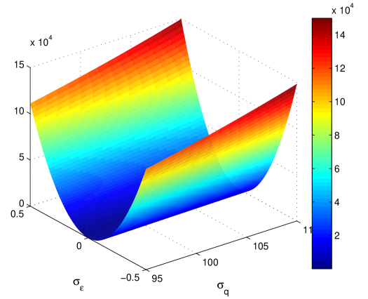
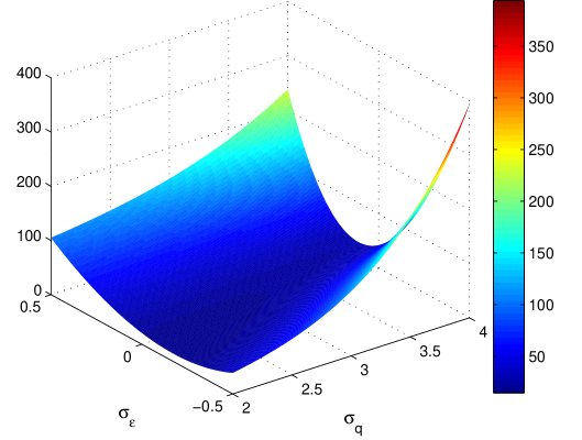
Figure 1: The 3D surfaces of the minimization function $F^{o}(\Xi)$: (left) $\sigma_{e}=0.0025,\sigma_{\nu}=0.0025$ (right) $\sigma_{e}=0.1,\sigma_{\nu}=0.1$

It is observed that for $n=5$ and $u_{m}=0$, the optimized value of $\sigma_{\epsilon}$ is close to zero or equal to zero, this is to say, the corresponding $s_{\epsilon}$ is close or equal to 2. When $\sigma_{e}$ and $\sigma_{\nu}$ are attenuated, numerically, $\sigma_{\epsilon}$ is equal to 0. However, the magnitude of $\sigma_{q}$ increases. Furthermore, the values of $F^{o}(\Xi)$ and $\mathcal{F}(\Xi)$ are around 17.9. In Fig. 1, the 3D surfaces of $F^{o}(\Xi)$ are displayed. From the figure, it is known that the function $F^{o}(\Xi)$ is convex and the extreme value can be found along $\sigma_{\epsilon}=0$. According to present numerical investigations, the value of $\sigma_{\epsilon}$ is always close or equal to 0. For the zero-mean flows, when $\sigma_{e}$ and $\sigma_{q}$ are specified, we can specify $\sigma_{\epsilon}$ equal to 0 or slightly larger than 0 in order to simplify the minimization problems for practical applications.

(a-1)                                                            (a-2)

(b-1)                                                            (b-2)

(c-1)                                                            (c-2)

(d-1)                                                            (d-2)

(e-1)                                                            (e-2)

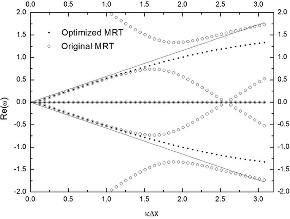
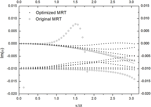
(f-1)                                                            (f-2)

Figure 2: Dispersion and dissipation profiles of the L-MRT-LBM based on recommended free parameters (except $s_{e}$ and $s_{\nu}$) [6] and optimized free parameters (group-A in Table 1). The relaxation parameters $s_{e}$ and $s_{\nu}$ are kept equal to those of the original MRT-LBM and the optimized MRT-LBM. The (#-1) figures display the dispersion profiles (magnified locally) and the straight lines represent the exact dispersion solutions. The (#-2) figures display the dissipation curves and the line is the expected shear mode and acoustic mode dissipation. The angle $\theta$ between the wavenumber $\bf k$ and the x-axis: (a) $\theta=0$;(b) $\theta=\pi/6$; (c) $\theta=\pi/4$; (d) $\theta=\pi/2$; (e) $\theta=2\pi/3$; (f) $\theta=3\pi/4$. (The symbol “#” stands for the characters a, b, c, d, e and f.)

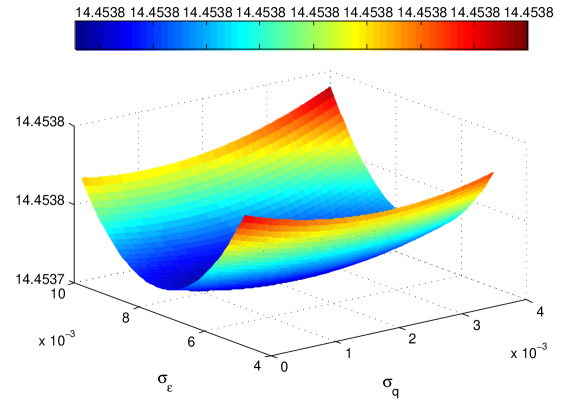
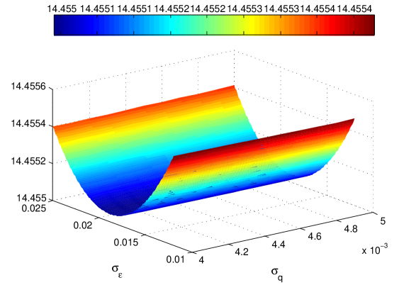
Figure 3: The 3D surfaces of the minimization function $\mathcal{F}^{o}(\Xi)$: (left) $\sigma_{e}=0.001,\sigma_{\nu}=0.001$; (right) $\sigma_{e}=0.0025,\sigma_{\nu}=0.0025$.

The Fig. 2 displays the dispersion and dissipation profiles of the L-MRT-LBM. In the original MRT-LBM, the free parameters $\sigma_{\epsilon}$ and $\sigma_{q}$ are taken equal to the recommended values [6] and the optimized free parameters are given by Group A in Table 1. From numerical results in Fig. 2, it is observed that when the wavenumber k is perpendicular or parallel to x-axis, the optimized MRT-LBM has the same dispersion relations as the original MRT-LBM. When $\theta$ is equal to other values, the optimized MRT-LBM performs better than the original MRT-LBM. These results also indicate that the cross derivatives in Eq. (37) are the main source of dispersion error. For the dissipation relations, it is observed that by the minimization problem, we can enhance the stability of the MRT-LBM. From the profiles of the dissipation relations, there exists one unstable mode the imaginary part ${\rm lm}(\omega)$ of which is larger than 0, when $0.75<k\Delta x<1.75$, $\theta\neq 0$ and $\theta\neq\pi/2$.

According to the definition of $\mathcal{M}_{\epsilon}$ in Sec. 3.2.2, we now consider $n=4$ and $u_{m}=0.1$ in Eqs. (37) and (59). Under these conditions, the dispersion and dissipation relations are investigated firstly. In Fig. (3), the 3D surfaces of $\mathcal{G}(\Xi)$ are shown. It is discovered that the function $\mathcal{G}(\Xi)$ is convex. Some optimized results for specified $\sigma_{e}$ and $\sigma_{\nu}$ are given in Table 2.

Table 2: Optimized free parameters for uniform flows ($u_{m}=0.1$) based on the perturbation matrix $\mathcal{M}_{\epsilon}$ in Sec. 3.2.2. The parameters are obtained by the minimization (71)

Groups	$\sigma_{e}=\sigma_{\nu}$	$\sigma_{\epsilon}$	$\sigma_{q}$	$\mathcal{G}(\Xi)$
A	0.001	0.00751873323089156	0.00171909400064198	14.4537555316616474
B	0.0025	0.0187982349323006	0.00429903714246050	14.4550408968152340

(a-1)                                                            (a-2)

(b-1)                                                            (b-2)

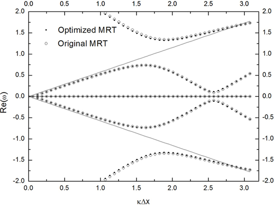
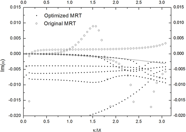
(c-1)                                                            (c-2)

Figure 4: Dispersion and dissipation profiles of the L-MRT-LBM based on recommended free parameters (except $s_{e}$ and $s_{\nu}$) [6] and optimized free parameters (group-A in Table 2). The relaxation parameters $s_{e}$ and $s_{\nu}$ are kept the same values for the original MRT-LBM and the optimized MRT-LBM. The (#-1) figures indicate the dispersion profiles (magnified locally) and the straight lines represent the exact dispersion solutions. The (#-2) figures indicate the dissipation curves and the line is the expected shear mode and acoustic mode dissipation. The angle $\vartheta=\pi/4$, $U=0.1$ and $V=0.1$. The angle $\widehat{\bf{k\cdot u}}$ between the wavenumber $\bf k$ and ${\bf u}$: (a) $\widehat{\bf{k\cdot u}}=0,\theta=\pi/4$;(b) $\widehat{\bf{k\cdot u}}=\pi/4,\theta=\pi$; (c) $\widehat{\bf{k\cdot u}}=\pi/2,\theta=3\pi/4$. (The symbol “#” stands for the characters a, b, and c.)

In Fig.4, we show the dispersion and dissipation profiles. It is seen that the best shear mode description is given by the optimization problem $\mathcal{G}(\Xi)$. At the same time, the optimized MRT-LBM is more stable than the original MRT-LBM. However, it is discovered that the dispersion error is not improved for $n=4$ by the minimization problem (71). If we want to reduce the influence of the non-zero mean flow on the dissipation relation and avoid handling lengthy mathematical expressions, it is suitable to choose $n=4$ in Eq. (37). Furthermore, when $\theta=\pi$, the optimized MRT-LBM has the similar dispersion and dissipation profiles with the original MRT-LBM in Fig. (4)-b. According to authors’ numerical investigations, when the angle $\theta$ is equal to $0$, $\pi/2$ and $\pi$, there always exist the similar dispersion and dissipation profiles between the optimized MRT-LBM and the original MRT-LBM. Based on the definition of $\mathcal{M}_{\epsilon}$ in Sec. 3.2.2, the results of numerical studies have shown that by the optimization problems (69), (70) and (71), the dispersion error was not reduced when $n<5$ in Eq. (37) for the uniform flows.

According to the definition of $\mathcal{M}_{\epsilon}$ in Sec. 3.2.3, we consider $n=4$ and $u_{m}=0.1$ in Eqs. (37) and (59). For very small shear and bulk viscosity parameters, we show some results in Table 3.

Table 3: Optimized free parameters for uniform flows ($u_{m}=0.1$) based on the perturbation matrix $\mathcal{M}_{\epsilon}$ in Sec. 3.2.3. The parameters are obtained by the minimization (71).

Group	$\sigma_{e}$	$\sigma_{\nu}$	$\sigma_{\epsilon}$	$\sigma_{q}$	$\mathcal{G}(\Xi)$
A	0.0025125628	0.00001	0.00947095595580122	0.00181622011980382	14.453655614637361
B	0.0000025	0.00001	0.0000311837523990053	0.00000760552251906507	14.45351071030945

In Figs. 5 and 6, the dispersion and dissipation relations are given for both the optimized MRT-LBM and the original MRT-LBM. It is discovered that, by the new definition of the perturbation matrix in Sec. 3.2.3, the optimized MRT-LBM is always stable for the very small viscosity and bulk viscosity. Furthermore, when the bulk viscosity (corresponding to Fig. 6) is very small, the numerical shear modes given by the optimized MRT-LBM agree with the exact shear modes very well. The obtained shear modes are nearly exact compared with the shear modes given by the original MRT-LBM. In order to observe the details of the optimized dissipation relations and the exact relations, in Fig. 7, the locally-magnified dissipation relations are given. It is clear that we observe a lower dissipation of the acoustic modes for the optimized MRT-LBM. From Figs. 5 and 6, it is also clear that when the bulk viscosity become smaller, the modes of the original MRT-LBM become more unstable for all values of the angle $\theta$. These results indicate that the original MRT-LBM is not suitable for aeroacoustic problems, because the bulk viscosity in the original MRT-LBM can not be chosen to be arbitrarily small. This limitation in the original MRT-LBM means that there exists a strong dissipation of the acoustic waves in the numerical simulations. The new definition of the perturbation matrix $\mathcal{M}_{\epsilon}$ in Sec. 3.2.3 coupled with the optimization strategy (71) overcomes this drawback of the MRT-LBM under the premise of guaranteeing the stability.

(a-1)                                                            (a-2)

(b-1)                                                            (b-2)

(c-1)                                                            (c-2)

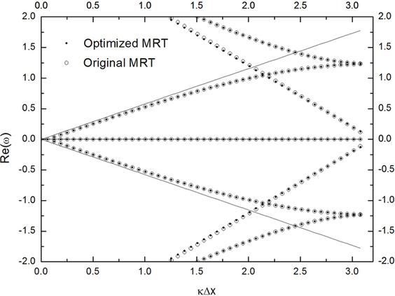
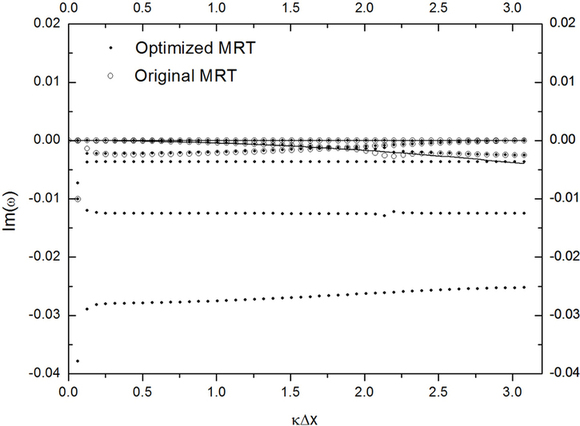
(d-1)                                                            (d-2)

Figure 5: Dispersion and dissipation profiles of the L-MRT-LBM based on recommended free parameters (except $s_{e}$ and $s_{\nu}$) [6] and optimized free parameters (group-A in Table 3). The relaxation parameters $s_{e}$ and $s_{\nu}$ are kept the same values for the original MRT-LBM and the optimized MRT-LBM. The (#-1) figures indicate the dispersion profiles (magnified locally) and the straight lines represent the exact dispersion solutions. The (#-2) figures indicate the dissipation curves and the lines are the expected shear mode and acoustic mode dissipation. The angle $\vartheta=\pi/4$, $U=0.1$ and $V=0.0$. The angle $\widehat{\bf{k\cdot u}}$ between the wavenumber $\bf k$ and ${\bf u}$: (a) $\widehat{\bf{k\cdot u}}=0,\theta=0$;(b) $\widehat{\bf{k\cdot u}}=\pi/3,\theta=\pi/3$; (c) $\widehat{\bf{k\cdot u}}=\pi/4,\theta=\pi/4$; (d) $\widehat{\bf{k\cdot u}}=\pi/2,\theta=\pi/2$. (The symbol “#” stands for the characters a, b, c and d.)

(a-1)                                                            (a-2)

(b-1)                                                            (b-2)

(c-1)                                                            (c-2)

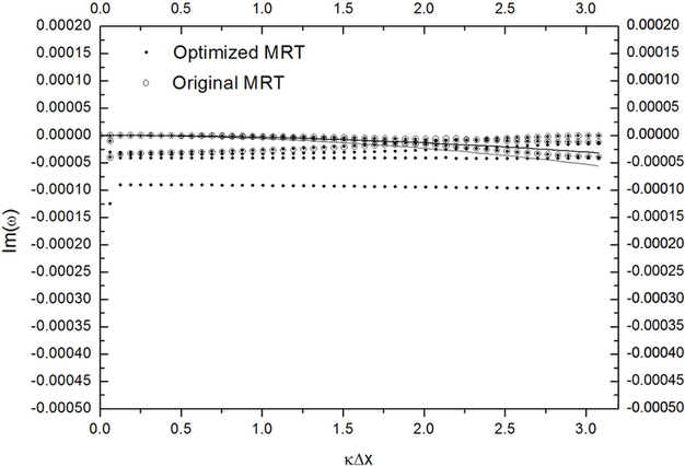
(d-1)                                                            (d-2)

Figure 6: Dispersion and dissipation profiles of the L-MRT-LBM based on recommended free parameters (except $s_{e}$ and $s_{\nu}$) [6] and optimized free parameters (group-B in Table 3). The relaxation parameters $s_{e}$ and $s_{\nu}$ are kept the same values for the original MRT-LBM and the optimized MRT-LBM. The (#-1) figures indicate the dispersion profiles (magnified locally) and the straight lines represent the exact dispersion solutions. The (#-2) figures indicate the dissipation curves and the lines are the expected shear mode and acoustic mode dissipation. The angle $\vartheta=\pi/4$, $U=0.1$ and $V=0.0$. The angle $\widehat{\bf{k\cdot u}}$ between the wavenumber $\bf k$ and ${\bf u}$: (a) $\widehat{\bf{k\cdot u}}=0,\theta=0$;(b) $\widehat{\bf{k\cdot u}}=\pi/3,\theta=\pi/3$; (c) $\widehat{\bf{k\cdot u}}=\pi/4,\theta=\pi/4$; (d) $\widehat{\bf{k\cdot u}}=\pi/2,\theta=\pi/2$. (The symbol “#” stands for the characters a, b, c and d.)

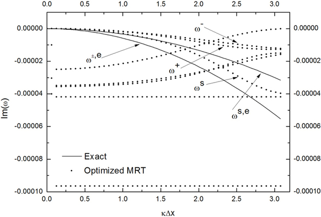
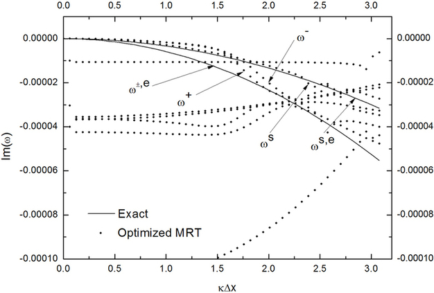
(a)                                                                     (b)

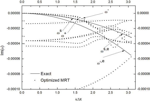
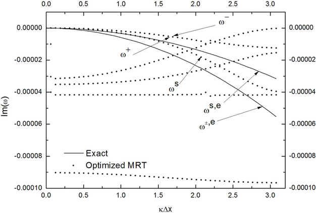
(c)                                                                     (d)

Figure 7: Locally-magnified dissipation profiles: Dissipation profiles of exact solutions (acoustic mode: $\omega^{\pm,{\rm e}}$; shear mode: $\omega^{\rm s,e}$) and optimized free parameters (group-B in Table 3; acoustic mode: $\omega^{\pm}$; shear mode: $\omega^{\rm s}$). The angle $\vartheta=\pi/4$, $U=0.1$ and $V=0.0$. The angle $\widehat{\bf{k\cdot u}}$ between the wavenumber $\bf k$ and ${\bf u}$: (a) $\widehat{\bf{k\cdot u}}=0,\theta=0$;(b) $\widehat{\bf{k\cdot u}}=\pi/3,\theta=\pi/3$; (c) $\widehat{\bf{k\cdot u}}=\pi/4,\theta=\pi/4$; (d) $\widehat{\bf{k\cdot u}}=\pi/2,\theta=\pi/2$.

5 Numerical simulations of acoustic problems

In this section, the classical acoustic problems will be simulated by optimized MRT-LBM. At the same time, some comparisons between the D2RP MRT-LBM and the original MRT-LBM are given.

5.1 Acoustic point source

In this part, we validate the optimized MRT-LBM by an acoustic point which sends out a sinusoidal signal [19, 20]. The point source is set by the following density configuration [19]

$$\rho({\rm x},t)=\rho_{0}+\rho_{s}{\rm sin}\left(\frac{2\pi}{T}t\right),$$ (79)

where $\rho_{s}$ is the point source amplitude, and $T$ the period of the oscillation with respect to lattice units. In order to avoid nonlinear wave effects, it is necessary that $\rho_{s}\ll\rho_{0}$. The macroscopic velocity $(u,v)$ at the point source is equal to 0.

Table 4: Specified relaxation parameters and optimized free relaxation parameters for zero-mean flows.

Groups	$s_{e}=s_{\nu}$	$s_{\epsilon}$	$s_{q}$	$\nu$	$\rho$	$\rho_{s}$
A	$1.99044751$	$2$	$0.00875438872$	$0.000799861$	1	0.01
B	1.95321	2	0.04126919093	0.00399257	1	0.01

Table 5: Specified parameters and optimized free parameters for uniform flows based on the perturbation matrix $\mathcal{M}_{\epsilon}$ in Sec. 3.2.3. The relaxation parameters are obtained by the minimization (71)

Groups	$s_{e}$	$s_{\nu}$	$s_{\epsilon}$	$s_{q}$
A	1.99	1.999960001	1.962820428	1.992761413
B	1.99999	1.999960001	1.999875273	1.999969578

It is known that the sound speed of the D2Q9 MRT-LBM is equal to $c_{s}=1/\sqrt{3}=0.57735$. In order to avoid the effects of boundaries, the wave propagation is limited in the computational domain $\Omega=100\times 100$. The lattice nodes are $101\times 101$ and the acoustic point source is set in the center of computational domain. So, if the lattice computational time $t$ is in the range $(0,\lfloor 50/c_{s}\rfloor]=(0,86]$, the wave will be limited in the domain $\Omega$. Now, we will use parameters given in Table 4 to validate the optimized MRT-LBM with the periodic boundary conditions.

In Figs. 8 and 9, the density contours and 3D surfaces are shown. Figs. 8(a) and 9(a) show that the optimized MRT-LBM corrects the anisotropy and annihilate the spurious fluctuations of waves. These results are better than the BGK-LBM and the original MRT-LBM. In Figs. 10 and 11, the waves along the line $y=51$ are given for three different methods at $t=80$ and $t=100$. It is clear that the optimized MRT-LBM is more effective than the BGK-LBM and the original MRT-LBM.

The numerical results demonstrate that by determining the free parameters, we can reduce the dispersion error and the isotropy error of the MRT-LBM.

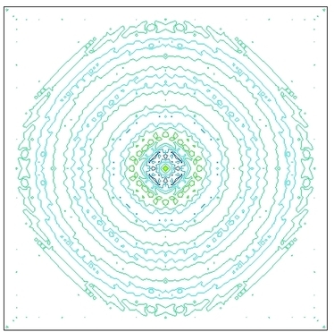
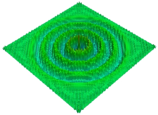
(a-1) $t=80$                                                             (a-2) $t=80$

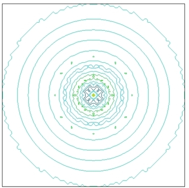
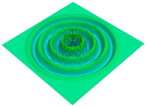
(b-1) $t=80$                                                             (b-2) $t=80$

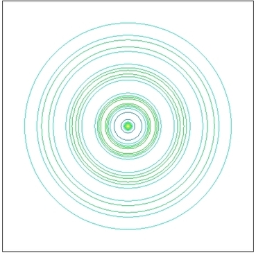
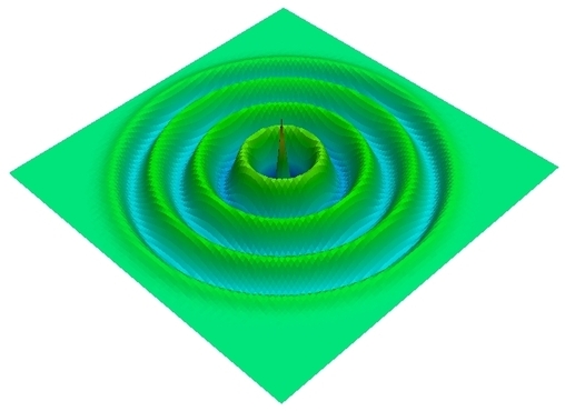
(c-1) $t=80$                                                             (c-2) $t=80$

Figure 8: The density contours (left figures) and the 3D surfaces (right figures) by the parameters of group-A in Table 4: (a) the BGK-LBM; (B) the original MRT-LBM; (C) the optimized MRT-LBM.

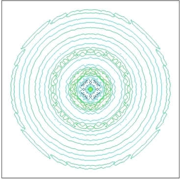
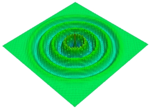
(a-1) $t=80$                                                             (a-2) $t=80$

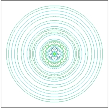
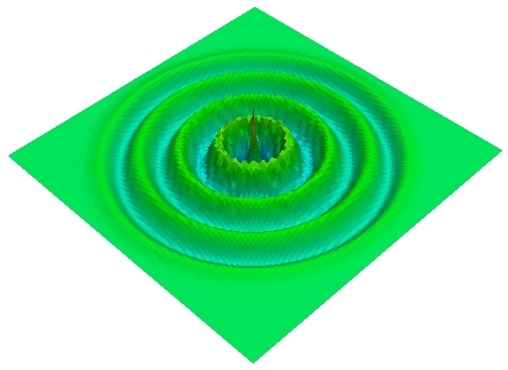
(b-1) $t=80$                                                              (b-2) $t=80$

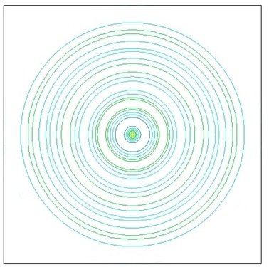
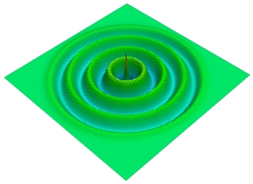
(b-1) $t=80$                                                             (b-2) $t=80$

Figure 9: The density contours (left figures) and the 3D surfaces (right figures) by the parameters of group-B in Table 4: (a) the BGK-LBM; (B) the original MRT-LBM; (C) the optimized MRT-LBM.

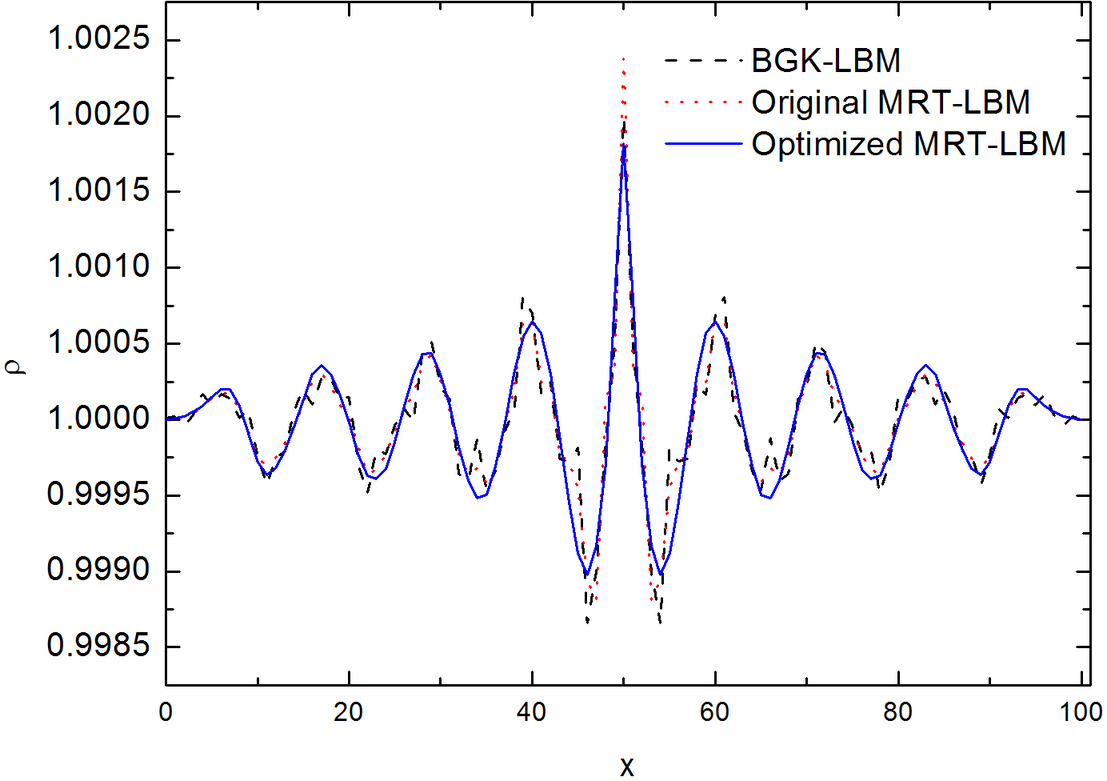
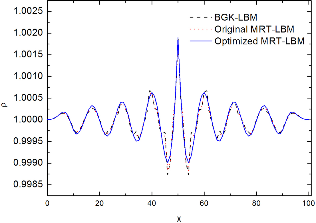
(a)                                                                     (b)

Figure 10: The comparisons of cross-profiles of the density $\rho$ at y=51 (the lattice time $t=80$): (a) Results obtained by the parameters of group-A in Table 4;(b) Results obtained by the parameters of group-B in Table 4.

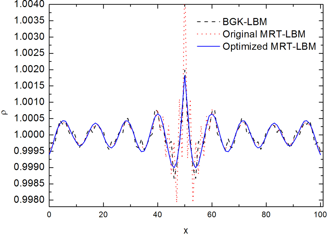
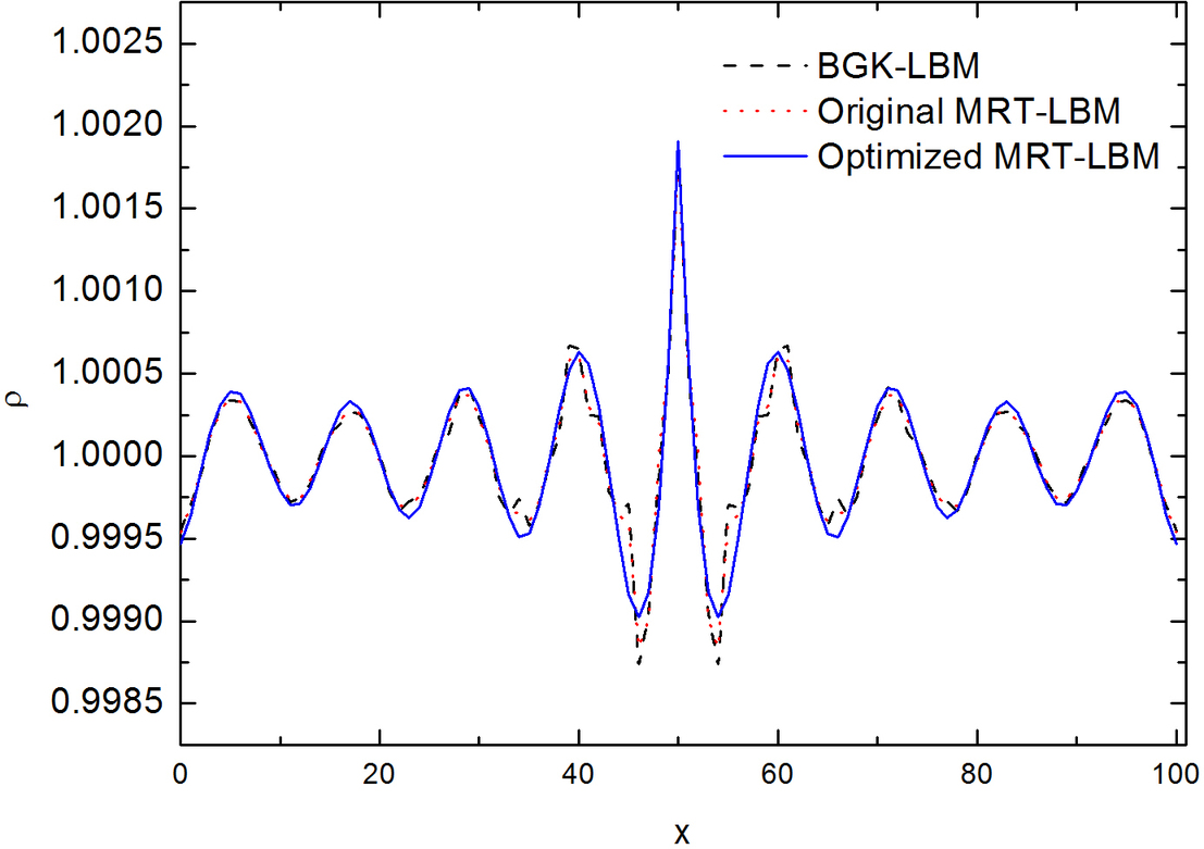
(a)                                                                     (b)

Figure 11: The comparisons of cross-profiles of the density $\rho$ at y=51 (the lattice time $t=100$):(a) Results obtained by the parameters of group-A in Table 4;(b) Results obtained by the parameters of group-B in Table 4.

5.2 Acoustic pressure pulse

In this part, the quality of the optimized MRT-LBM is assessed considering the acoustic pressure pulse problem. These comparisons provide an evidence for the accuracy of computed solutions. In order to compare the results with the exact solution and neglect the effects of the dissipation, the very small values of shear and bulk viscosity are chosen for a MRT-LBM. The initial perturbation is given by a Gaussian density distribution at the center of the domain at $t=0$ [11]

$$\left\{\begin{array}[]{rl}\rho(x,y,0)&=\rho_{0}+\varepsilon\mathrm{exp}(-\alpha\eta^{2}),\\ u(x,y,0)&=U_{0},\\ v(x,y,0)&=0,\end{array}\right.$$ (80)

where $\alpha$ is related to the half-width Gaussian , $b$, by $\alpha=\mathrm{ln}2/b^{2}$. $\eta$ is defined by $\eta=\left[(x-U_{0}t)^{2}+y^{2}\right]$, which is equal to the radial coordinate at $t=0$. $\varepsilon$ is the density pulse amplitude. The analytical solution of the problem for the pressure and density can be given by a zero-order Bessel function $J_{0}$ [11]

$$\rho(x,y,t)=\rho_{0}+\frac{\varepsilon}{2\alpha}\int_{0}^{\infty}\mathrm{exp}(-\xi^{2}/(4\alpha))\mathrm{cos}(c_{s}\xi t)J_{0}(\xi\eta)\xi\mathrm{d}\xi.$$ (81)

It is noted that Eq. (81) does not include the dissipation introduced by the viscosity of the fluid. So, in order to implement the computation, the influence of viscosity on pressure wave must be minimized by the small magnitude of viscosity. The computational domain is $[0,1]\times[0,1]$. The parameters $\varepsilon$ and $b$ are equal to 0.01 and 0.04, respectively. In Figs. 12 and 13, we show the horizontal density profiles at y=0.5. The simulation physical time $t=0.4$. From these figures, it is clear that the results by the optimized MRT-LBM are superior to the results by the original MRT-LBM. Obviously, the amplitudes of crests and troughs are damped by the bulk viscosity in the original MRT-LBM. It is demonstrated that by the proposed strategy (71) and the new definition of $\mathcal{M}_{\epsilon}$ in Sec. 3.2.3, the dissipation influence from the bulk viscosity on pressure waves can be reduced to a negligible level. Meanwhile, the bulk viscosity can be attenuated. In Fig. 14, the figures of density distribution are given. In order to test the accuracy, the following $L^{2}$-norm relative error is defined

$$E_{L^{2}}=\sqrt{\frac{\sum_{i=1}^{N_{\rm nodes}}{(\rho_{i}^{\rm th}-\rho_{i}^{\rm num})^{2}}}{\sum_{i=1}^{N_{\rm nodes}}(\rho_{i}^{\rm th})^{2}}},$$ (82)

where $\rho_{i}^{\rm th}$ and $\rho_{i}^{\rm num}$ denote the theoretical and numerical solutions, respectively. In Fig. 15, the $L^{2}$-norm relative errors of density are given based on lattice nodes in a log-log coordinate. From this figure, it is discovered that the convergence orders of pressure pulse for the optimized MRT-LBM and the original MRT-LBM are very close to 1. However, the result given by the optimized MRT-LBM are better than that given by the original MRT-LBM.

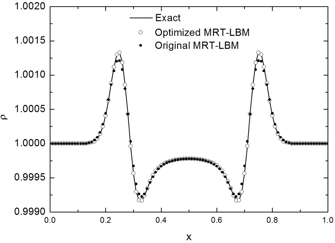
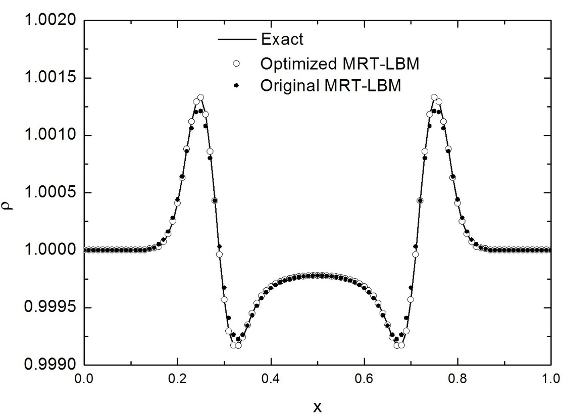
(a) Horizontal density profiles at y=0.5                 (b) Horizontal density profiles at y=0.5

Figure 12: The comparisons of the cross profiles of the density $\rho$ at y=0.5: The horizontal velocity $U_{0}=0$. (a) The results of the optimized MRT-LBM are obtained by the parameters of group-A in Table 5 (b) The results of the optimized MRT-LBM are obtained by the parameters of group-B in Table 5. (The computational physical time $t=0.4$)

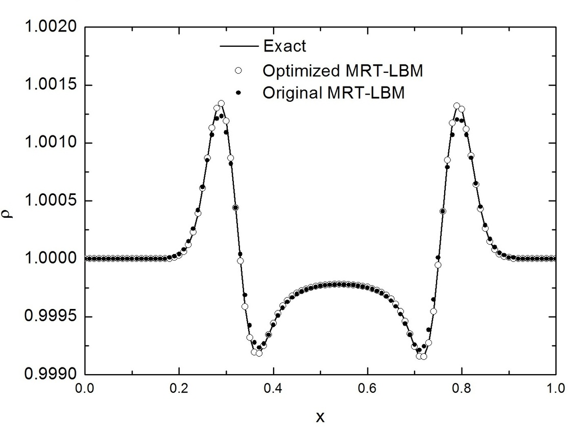
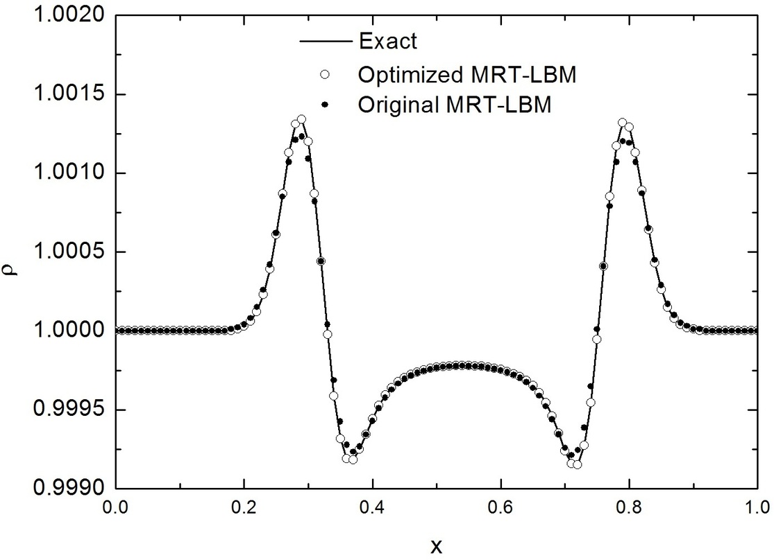
(a) Horizontal density profiles at y=0.5                 (b) Horizontal density profiles at y=0.5

Figure 13: The comparisons of the cross profiles of the density $\rho$ at y=0.5: The horizontal velocity $U_{0}=0.1$. (a) The results of the optimized MRT-LBM are obtained by the parameters of group-A in Table 5 (b) The results of the optimized MRT-LBM are obtained by the parameters of group-B in Table 5. (The computational physical time $t=0.4$)

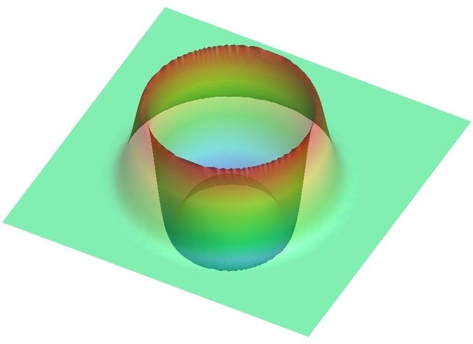
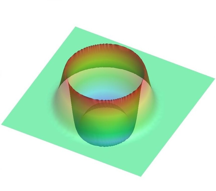
(a) Density distribution by the optimized MRT-LBM           (b) Density profiles by the original MRT-LBM.

Figure 14: The comparisons of density distribution with the horizontal velocity $U_{0}=0.1$. (a) The results of the optimized MRT-LBM are obtained by the parameters of group-A in Table 5 (b) The results of the original MRT-LBM. (The computational physical time $t=0.4$)

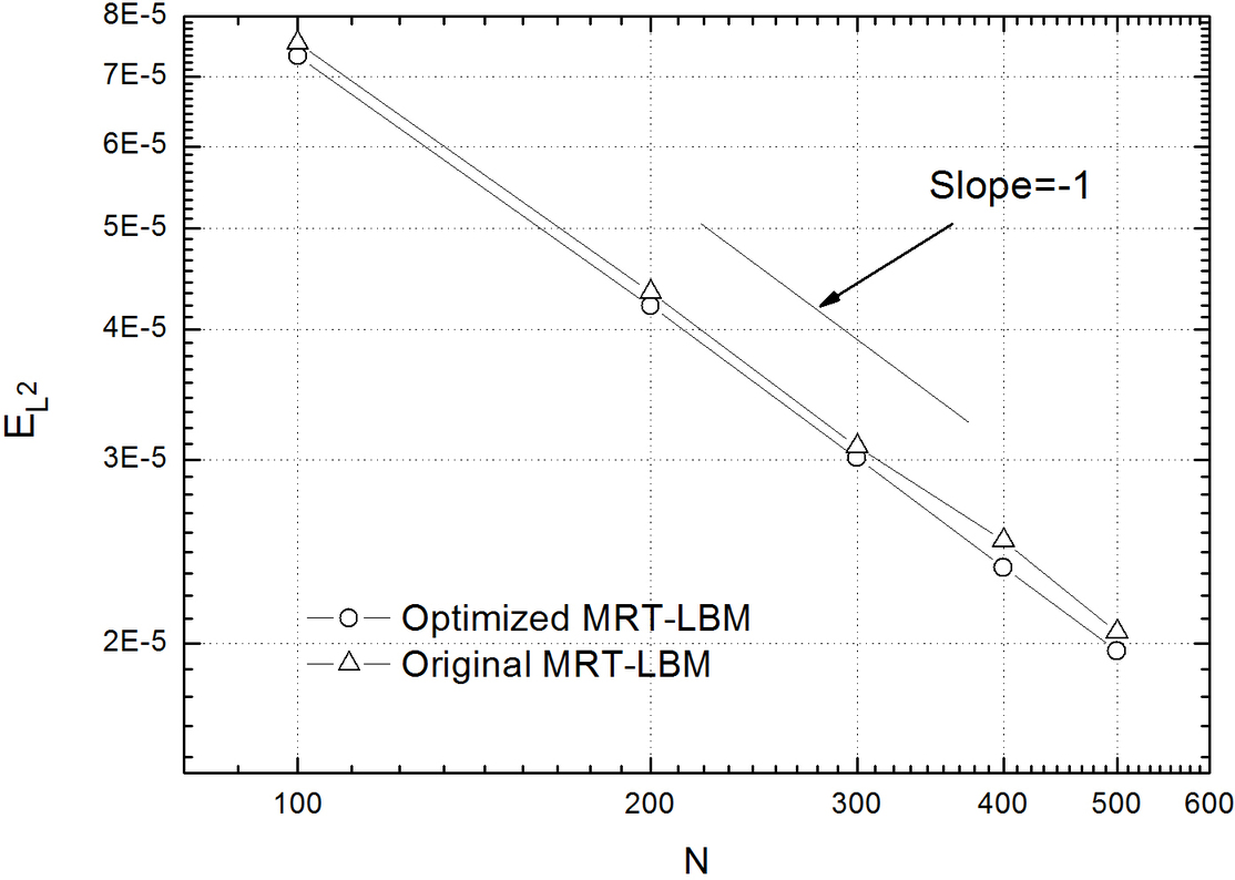
Figure 15: The comparisons of relative errors of the density $\rho$ in the log-log coordinate. The results of the optimized MRT-LBM are obtained by the parameters of group-A in Table 5 (The computational physical time $t=0.4$)

6 Conclusion

In this paper, we have proposed several numerical strategies to reduce the dispersion/dissipation errors (regarded the optimized MRT-LBM as the D2PR-LBM). We also gave an easy-to-use algorithm to derive linearized Navier-Stokes with the high-order truncation errors starting from the linearized MRT-LBM. Von Neumann analysis of the isothermal linearized MRT-LBM and the linearized BGK-LBM has been made to investigate the dispersion and dissipation relations. The von Neumann stability analysis also shows that by optimizing free parameters, the acoustic modes are decoupled from the shear modes and other modes with respect to zero-mean flows when the truncation error is up to $O(\delta t^{5})$. For uniform flows, it is discovered that when the truncation error is up to $O(\delta t^{4})$, by optimization strategies, the dissipation error can only be reduced and the influences from mean flows on dissipation relations are also reduced. The stability of the MRT-LBM is enhanced. Especially, when the shear viscosity and bulk viscosity are very small, the optimized dissipation relation is nearly exact. The optimized MRT-LBM can annihilate the spurious waves and the isotropic error suffered by the original MRT-LBM and reduce the over-damping influence of the bulk viscosity on pressure waves. Numerical simulations of acoustic problems demonstrated that for acoustic problems, the optimized MRT-LBM is more effective than the original MRT-LBM.

Appendix A The Taylor expansion strategy of the L-MRT-LBM in wave-number spaces

In this part, we show the derivation details from the L-MRT-LBM to the L-NSE and the truncation error is up to $O(\delta t^{4})$.
(1) When $J=1$ in Eq. (23), we have

$$W_{i}=m_{i},0\leq i\leq d,$$ (83)

$$m_{i}=\frac{1}{s_{i}}\Psi_{ij}W_{j}+O(\delta t),d<i\leq N.$$ (84)

We rewrite Eqs. (83) and (84) as a uniform expression

$$m_{i}=\Phi_{ij,1}W_{j}+O(\delta t),0\leq i\leq N,$$ (85)

where

$$\Phi_{ij,1}=\delta_{ij}(0\leq i\leq d),\Phi_{ij,1}=\frac{1}{s_{i}}\Psi_{ij}(d+1\leq i\leq N).$$ (86)

(2) When $J=2$ in Eq. (23), we have

$$m_{i}+\delta t\partial_{t}m_{i}=A_{ir,0}m_{r}+\delta tA_{ir,1}m_{r}+O(\delta t^{2}).$$ (87)

When $0\leq i\leq d$, we have

$$W_{i}+\delta t\partial_{t}W_{i}=A_{ir,0}m_{r}+\delta tA_{ir,1}m_{r}+O(\delta t^{2}).$$ (88)

Because $A_{ir,0}=\delta_{ir}$, we have

$$W_{i}+\delta t\partial_{t}W_{i}=\delta_{ir}m_{r}+\delta tA_{ir,1}m_{r}+O(\delta t^{2}).$$ (89)

That is,

$$\partial_{t}W_{i}=A_{ir,1}m_{r}+O(\delta t).$$ (90)

According to Eq. (85), we have

$$\partial_{t}W_{i}=A_{ir,1}\Phi_{rj,1}W_{j}+O(\delta t).$$ (91)

Let

$$B_{ij,1}=A_{ir,1}\Phi_{rj,1}.$$ (92)

Then, we obtain

$$\partial_{t}W_{i}=B_{ij,1}W_{j}+O(\delta t).$$ (93)

When $d+1\leq i\leq N$, we have

$$m_{i}+\delta t\partial_{t}m_{i}=A_{ir,0}m_{r}+\delta tA_{ir,1}m_{r}+O(\delta t^{2}).$$ (94)

It is known that when $d+1\leq i\leq N$, $A_{ir,0}$ is defined by [8]

$$A_{ir,0}m_{r}=(\delta_{ir}-S_{ir})m_{r}-\Psi_{ij}W_{j}.$$ (95)

So, we have (the combination of Eqs. (95) and (84))

$$m_{i}+\delta t\Phi_{ij,1}\partial_{t}W_{j}=(\delta_{ir}-S_{ir})m_{r}-\Psi_{ij}W_{j}+\delta tA_{ir,1}\Phi_{rj,1}W_{j}+O(\delta t^{2}),$$ (96)

$$m_{i}=\frac{1}{s_{i}}(-\Psi_{ij}-\delta t\Phi_{ik,1}B_{kj,1}+\delta tA_{ir,1}\Phi_{rj,1})W_{j}+O(\delta t^{2}).$$ (97)

Now, introducing $\Phi_{ij,2}$ as follows

$$\Phi_{ij,2}=\delta_{ij}(0\leq i\leq d),$$ (98)

we have

$$\Phi_{ij,2}=\frac{1}{s_{i}}(-\delta t\Phi_{ik,1}B_{kj,1}+\Psi_{ij}+\delta tA_{ir,1}\Phi_{rj,1}),(d+1\leq i\leq N).$$ (99)

So, we obtain

$$m_{i}=\Phi_{ij,2}W_{j}+O(\delta t^{2}).$$ (100)

(3) When $J=3$ in Eq. (23), we have

$$m_{i}+\delta t\partial_{t}m_{i}+\frac{\delta t^{2}}{2!}\partial_{t}m_{i}=A_{ir,0}m_{r}+\delta tA_{ir,1}m_{r}+\delta t^{2}A_{ir,2}m_{r}+O(\delta t^{3}).$$ (101)

When $0\leq i\leq d$, we have

$$\partial_{t}W_{i}+\frac{\delta t}{2!}\partial_{t}W_{i}=A_{ir,1}m_{r}+\delta tA_{ir,2}m_{r}+O(\delta t^{2}).$$ (102)

By Eqs. (93), (85) and (100), we get

$$\partial_{t}W_{i}=-\frac{\delta t}{2!}B_{ij,1}W_{j}+A_{ir,1}\Phi_{rj,2}W_{j}+\delta tA_{ir,2}\Phi_{rj,1}W_{j}+O(\delta t^{2}).$$ (103)

Let

$$B_{ij,2}=-\frac{\delta t}{2!}B_{ij,1}W_{j}+A_{ir,1}\Phi_{rj,2}W_{j}+\delta tA_{ir,2}\Phi_{rj,1},$$ (104)

we get

$$\partial_{t}W_{i}=B_{ij,2}W_{j}+O(\delta t^{2})$$ (105)

When $d+1\leq i\leq N$, by Eqs.(100), (85) and (105), we have

$$m_{i}=\frac{1}{s_{i}}(-\delta t\Phi_{ik,2}B_{kj,2}-\frac{\delta t^{2}}{2!}\Phi_{ik,1}B_{kj,1}^{2}+\Psi_{ij}+\delta tA_{ir,1}\Phi_{rj,2}+\frac{\delta t^{2}}{2!}A_{ir,2}\Phi_{rj,1})W_{j}+O(\delta t^{3}).$$ (106)

Now, introducing $\Phi_{ij,3}$, we get

$$\Phi_{ij,3}=\delta_{ij}(0\leq i\leq d),$$

and for $(d+1\leq i\leq N)$

$$\Phi_{ij,3}=\frac{1}{s_{i}}(-\delta t\Phi_{ik,2}B_{kj,2}-\frac{\delta t^{2}}{2!}\Phi_{ik,1}B_{kj,1}^{2}+\Psi_{ij}+\delta tA_{ir,1}\Phi_{rj,2}+\delta t^{2}A_{ir,2}\Phi_{rj,1}).$$ (107)

In order to restrict the truncated error of Eq. (107) equal to $O(\delta t^{3})$, we rewrite Eq. (107) as follows

$$\Phi_{ij,3}=\sum_{l=0}^{2}\delta t^{l}{\rm Coeff}(\Phi_{ij,3},\delta t,l).$$

So, we have

$$m_{i}=\Phi_{ij,3}W_{j}+O(\delta t^{3}).$$ (108)

(4) When $J=4$ in Eq. (23), we have

$$m_{i}+\delta t\partial_{t}m_{i}+\frac{\delta t^{2}}{2!}\partial_{t}^{2}m_{i}+\frac{\delta t^{3}}{3!}\partial_{t}^{3}m_{i}=A_{ir,0}m_{r}+\delta tA_{ir,1}m_{r}+\delta t^{2}A_{ir,2}m_{r}+\delta t^{3}A_{ir,3}m_{r}+O(\delta t^{4}).$$ (109)

When $0\leq i\leq d$, we have

$$\partial_{t}W_{i}+\frac{\delta t}{2!}\partial_{t}^{2}W_{i}+\frac{\delta t^{2}}{3!}\partial_{t}^{3}W_{i}=A_{ir,1}m_{r}+\delta tA_{ir,2}m_{r}+\delta t^{2}A_{ir,3}m_{r}+O(\delta t^{3}).$$ (110)

By Eqs. (108), (105) and (93), we get the R.H.S of Eq. (110),

$${\rm R.H.S}=A_{ir,1}\Phi_{rj,3}W_{j}+\delta tA_{ir,2}\Phi_{rj,2}W_{j}+\delta t^{2}A_{ir,3}B_{rj,1}W_{j}+O(\delta t^{3}).$$ (111)

By Eqs. (105) and (93), we get the L.H.S of Eq. (110),

$${\rm L.H.S}=\partial_{t}W_{i}+\frac{\delta t}{2!}B_{ij,2}^{2}W_{j}+\frac{\delta t^{2}}{3!}B_{ij,1}^{3}W_{j}.$$ (112)

So, we have

$$\partial_{t}W_{i}=(-\frac{\delta t}{2!}B_{ij,2}^{2}-\frac{\delta t^{2}}{3!}B_{ij,1}^{3}+A_{ir,1}\Phi_{rj,3}+\delta tA_{ir,2}\Phi_{rj,2}+\delta t^{2}A_{ir,3}\Phi_{rj,1})W_{j}+O(\delta t^{3}).$$ (113)

Let

$$B_{ij,3}=-\frac{\delta t}{2!}B_{ij,2}^{2}-\frac{\delta t^{2}}{3!}B_{ij,1}^{3}+A_{ir,1}\Phi_{rj,3}+\delta tA_{ir,2}\Phi_{rj,2}+\delta t^{2}A_{ir,3}\Phi_{rj,1},$$ (114)

we restrict the truncated error of Eq. (114) equal to $O(\delta t^{3})$ and get

$$B_{ij,3}=\sum_{l=0}^{2}\delta t^{l}{\rm Coeff}(B_{ij,3},\delta t,l).$$ (115)

Then, we have

$$\partial_{t}W_{i}=B_{ij,3}W_{j}+O(\delta t^{3}).$$ (116)

When $d+1\leq i\leq N$, we have

$$m_{i}+\delta t\partial_{t}m_{i}+\frac{\delta t^{2}}{2!}\partial_{t}^{2}m_{i}+\frac{\delta t^{3}}{3!}\partial_{t}^{3}m_{i}=A_{ir,0}m_{r}+\delta tA_{ir,1}m_{r}+\delta t^{2}A_{ir,2}m_{r}+\delta t^{3}A_{ir,3}m_{r}+O(\delta t^{4}).$$ (117)

By Eqs. (85), (93), (100), (105), (108) and (116), we get the L.H.S of Eq. (109)

$${\rm L.H.S}=m_{i}+\delta t\Phi_{ir,3}B_{rj,3}W_{j}+\frac{\delta t^{2}}{2!}\Phi_{ir,2}B_{rj,2}^{2}W_{j}+\frac{\delta t^{3}}{3!}\Phi_{ir,1}B_{rj,1}^{3}W_{j}.$$ (118)

By Eqs. (116), (105) and (85), we gain the R.H.S of Eq. (109)

$${\rm R.H.S}=(1-s_{i})m_{i}+\Psi_{ij}W_{j}+\delta tA_{ir,1}\Phi_{rj,3}W_{j}+\delta t^{2}A_{ir,2}\Phi_{rj,2}W_{j}+\delta t^{3}A_{ir,3}\Phi_{rj,1}W_{j}+O(\delta t^{4}).$$ (119)

So, we have

$$m_{i}=\frac{1}{s_{i}}(-\delta t\Phi_{ir,3}B_{rj,3}-\frac{\delta t^{2}}{2!}\Phi_{ir,2}B_{rj,2}^{2}-\frac{\delta t^{3}}{3!}\Phi_{ir,1}B_{rj,1}^{3}+\Psi_{ij}+\delta tA_{ir,1}\Phi_{rj,3}+\delta t^{2}A_{ir,2}\Phi_{rj,2}+\delta t^{3}A_{ir,3}\Phi_{rj,1})W_{j}+O(\delta t^{4}).$$ (120)

Let

$$\Phi_{ij,4}=\delta_{ij}(0\leq i\leq d),$$

and for $d+1\leq i\leq N$

$$\Phi_{ij,4}=\frac{1}{s_{i}}(-\delta t\Phi_{ir,3}B_{rj,3}-\frac{\delta t^{2}}{2!}\Phi_{ir,2}B_{rj,2}^{2}-\frac{\delta t^{3}}{3!}\Phi_{ir,1}B_{rj,1}^{3}+\Psi_{ij}+\delta tA_{ir,1}\Phi_{rj,3}+\delta t^{2}A_{ir,2}\Phi_{rj,2}+\delta t^{3}A_{ir,3}\Phi_{rj,1}),$$ (121)

and we restrict the truncated error of Eq. (121) equal to $O(\delta t^{4})$ and get

$$\Phi_{ij,4}=\sum_{l=0}^{3}\delta t^{l}{\rm Coeff}(\Phi_{ij,4},\delta t,l).$$

So, we have

$$m_{j}=\Phi_{ij,4}W_{j}+O(\delta t^{4}).$$ (122)

Appendix B The coefficient matrices of the higher-order L-NSE with the zero-mean flow

(A) The coefficients of $\delta t^{2}$ are given by the following matrix

$$\mathrm{i}\cdot\left[\begin{array}[]{ccc}0&-\frac{1}{18}\,{k_{x}}\,\left({{k_{x}}}^{2}+{{k_{y}}}^{2}\right)&-\frac{1}{18}\,{k_{y}}\,\left({{k_{x}}}^{2}+{{k_{y}}}^{2}\right)\\ \vskip 6.0pt plus 2.0pt minus 2.0pt\cr-\frac{1}{27}\,{k_{x}}\,\left(-{{k_{x}}}^{2}-{{k_{y}}}^{2}+3\,{{k_{y}}}^{2}{\sigma_{e}}^{2}+3\,{{k_{x}}}^{2}{\sigma_{e}}^{2}+3\,{{k_{y}}}^{2}{\sigma_{\nu}}^{2}+3\,{{k_{x}}}^{2}{\sigma_{\nu}}^{2}\right)&0&0\\ \vskip 6.0pt plus 2.0pt minus 2.0pt\cr-\frac{1}{27}\,{k_{y}}\,\left(-{{k_{x}}}^{2}-{{k_{y}}}^{2}+3\,{{k_{y}}}^{2}{\sigma_{e}}^{2}+3\,{{k_{x}}}^{2}{\sigma_{e}}^{2}+3\,{{k_{y}}}^{2}{\sigma_{\nu}}^{2}+3\,{{k_{x}}}^{2}{\sigma_{\nu}}^{2}\right)&0&0\end{array}\right]$$ (123)

(B) The coefficients of $\delta t^{3}$ are given by the following matrix

$${\rm Coeff}(B_{,5}[1,1],\delta t^{3})={\frac{1}{108}}\,{{k_{y}}}^{4}\sigma_{e}+{\frac{1}{54}}\,{{k_{x}}}^{2}{{k_{y}}}^{2}\sigma_{e}+{\frac{1}{108}}\,{{k_{x}}}^{4}\sigma_{e}+{\frac{1}{108}}\,{{k_{y}}}^{4}\sigma_{\nu}+{\frac{1}{108}}\,{{k_{x}}}^{4}\sigma_{\nu}+{\frac{1}{54}}\,{{k_{x}}}^{2}{{k_{y}}}^{2}\sigma_{\nu}$$ (124)

$${\rm Coeff}(B_{,5}[1,2],\delta t^{3})=0,{\rm Coeff}(B_{,5}[1,3],\delta t^{3})=0,{\rm Coeff}(B_{,5}[2,1],\delta t^{3})=0$$ (125)

$$\begin{array}[]{r}{\rm Coeff}(B_{,5}[2,2],\delta t^{3})=-\frac{5}{9}\,{{k_{x}}}^{2}{{k_{y}}}^{2}\sigma_{\nu}\,\sigma_{\epsilon}\,\sigma_{q}+\frac{1}{9}\,{{k_{x}}}^{4}\sigma_{\epsilon}\,\sigma_{q}\,\sigma_{\nu}+{\frac{5}{18}}\,{{k_{x}}}^{2}{{k_{y}}}^{2}{\sigma_{\nu}}^{2}\sigma_{q}-1/9\,{{k_{x}}}^{2}{{k_{y}}}^{2}{\sigma_{\nu}}^{2}\sigma_{e}-{\frac{5}{54}}\,{{k_{x}}}^{2}{{k_{y}}}^{2}\sigma_{\nu}-\\[5.69054pt] {\frac{13}{108}}\,{{k_{x}}}^{2}{{k_{y}}}^{2}\sigma_{e}-\frac{1}{9}\,{{k_{x}}}^{4}\sigma_{\nu}\,{\sigma_{e}}^{2}+\frac{1}{6}\,{{k_{x}}}^{4}{\sigma_{e}}^{2}\sigma_{q}-{\frac{1}{108}}\,{{k_{x}}}^{4}\sigma_{\nu}-{\frac{1}{108}}\,{{k_{x}}}^{4}\sigma_{e}-\frac{1}{9}\,{{k_{x}}}^{4}\sigma_{e}\,\sigma_{\epsilon}\,\sigma_{q}-\frac{1}{9}\,{{k_{x}}}^{2}{{k_{y}}}^{2}\sigma_{e}\,\sigma_{\epsilon}\,\sigma_{q}-\\[5.69054pt] \frac{1}{36}\,{{k_{y}}}^{4}\sigma_{\nu}-\frac{1}{9}\,{{k_{y}}}^{4}{\sigma_{\nu}}^{3}+{\frac{10}{9}}\,{{k_{x}}}^{2}{{k_{y}}}^{2}\sigma_{\nu}\,\sigma_{e}\,\sigma_{q}-\frac{2}{9}\,{{k_{x}}}^{4}\sigma_{\nu}\,\sigma_{e}\,\sigma_{q}+\frac{1}{6}\,{{k_{x}}}^{2}{{k_{y}}}^{2}{\sigma_{e}}^{2}\sigma_{q}-\frac{1}{9}\,{{k_{x}}}^{2}{{k_{y}}}^{2}{\sigma_{e}}^{2}\sigma_{\nu}+\frac{1}{18}\,{{k_{x}}}^{4}{\sigma_{\nu}}^{2}\sigma_{q}-\\[5.69054pt] \frac{1}{9}\,{{k_{x}}}^{4}{\sigma_{\nu}}^{2}\sigma_{e}-\frac{1}{9}\,{{k_{x}}}^{2}{{k_{y}}}^{2}{\sigma_{\nu}}^{3}+\frac{2}{9}\,{{k_{y}}}^{4}{\sigma_{\nu}}^{2}\sigma_{q}+\frac{1}{18}\,{{k_{x}}}^{2}{{k_{y}}}^{2}\sigma_{\epsilon}\end{array}$$ (126)

$$\begin{array}[]{r}{\rm Coeff}(B_{,5}[2,3],\delta t^{3})=\frac{1}{6}\,{k_{x}}\,{{k_{y}}}^{3}{\sigma_{\nu}}^{2}\sigma_{q}-\frac{5}{9}\,{k_{x}}\,{{k_{y}}}^{3}\sigma_{\nu}\,\sigma_{\epsilon}\,\sigma_{q}-\frac{1}{9}\,{k_{x}}\,{{k_{y}}}^{3}\sigma_{e}\,\sigma_{\epsilon}\,\sigma_{q}+\frac{1}{6}\,{{k_{x}}}^{3}{k_{y}}\,{\sigma_{\nu}}^{2}\sigma_{q}+\frac{1}{9}\,{{k_{x}}}^{3}{k_{y}}\,\sigma_{\epsilon}\,\sigma_{q}\,\sigma_{\nu}-\\[5.69054pt] \frac{1}{9}\,{{k_{x}}}^{3}{k_{y}}\,\sigma_{e}\,\sigma_{\epsilon}\,\sigma_{q}+\frac{1}{6}\,{k_{x}}\,{{k_{y}}}^{3}{\sigma_{e}}^{2}\sigma_{q}+{\frac{7}{9}}\,{k_{x}}\,{{k_{y}}}^{3}\sigma_{\nu}\,\sigma_{e}\,\sigma_{q}+\frac{1}{6}\,{{k_{x}}}^{3}{k_{y}}\,{\sigma_{e}}^{2}\sigma_{q}+\frac{1}{9}\,{{k_{x}}}^{3}{k_{y}}\,\sigma_{e}\,\sigma_{\nu}\,\sigma_{q}-{\frac{5}{54}}\,{k_{x}}\,{{k_{y}}}^{3}\sigma_{e}-\\[5.69054pt] {\frac{7}{108}}\,{k_{x}}\,{{k_{y}}}^{3}\sigma_{\nu}-{\frac{7}{108}}\,{{k_{x}}}^{3}{k_{y}}\,\sigma_{\nu}-\frac{1}{27}\,{{k_{x}}}^{3}{k_{y}}\,\sigma_{e}-\frac{1}{9}\,{k_{x}}\,{{k_{y}}}^{3}{\sigma e}^{2}\sigma_{\nu}+\frac{1}{9}\,{{k_{x}}}^{3}{k_{y}}\,{\sigma_{\nu}}^{3}+\frac{1}{9}\,{k_{x}}\,{{k_{y}}}^{3}{\sigma_{\nu}}^{3}-\frac{1}{9}\,{{k_{x}}}^{3}{k_{y}}\,{\sigma_{\nu}}^{2}\sigma_{e}+\\[5.69054pt] \frac{1}{18}\,{k_{x}}\,{{k_{y}}}^{3}\sigma_{\epsilon}-\frac{1}{9}\,{{k_{x}}}^{3}{k_{y}}\,\sigma_{\nu}\,{\sigma_{e}}^{2}-\frac{1}{9}\,{k_{x}}\,{{k_{y}}}^{3}{\sigma_{\nu}}^{2}\sigma_{e}\end{array}$$ (127)

$${\rm Coeff}(B_{,5}[3,1],\delta t^{3})=0$$ (128)

$$\begin{array}[]{r}{\rm Coeff}(B_{,5}[3,2],\delta t^{3})=\frac{1}{18}\,{{k_{x}}}^{3}{k_{y}}\,\sigma_{\epsilon}-\frac{5}{9}\,{{k_{x}}}^{3}{k_{y}}\,\sigma_{\epsilon}\,\sigma_{q}\,\sigma_{\nu}+\frac{1}{9}\,{k_{x}}\,{{k_{y}}}^{3}\sigma_{\nu}\,\sigma_{\epsilon}\,\sigma_{q}-\frac{1}{9}\,{k_{x}}\,{{k_{y}}}^{3}\sigma_{e}\,\sigma_{\epsilon}\,\sigma_{q}-\frac{1}{9}\,{{k_{x}}}^{3}{k_{y}}\,\sigma_{e}\,\sigma_{\epsilon}\,\sigma_{q}+\\[5.69054pt] \frac{1}{6}\,{{k_{x}}}^{3}{k_{y}}\,{\sigma_{\nu}}^{2}\sigma_{q}-\frac{1}{9}\,{{k_{x}}}^{3}{k_{y}}\,\sigma_{\nu}\,{\sigma_{e}}^{2}-\frac{1}{27}\,{k_{x}}\,{{k_{y}}}^{3}\sigma_{e}-{\frac{7}{108}}\,{k_{x}}\,{{k_{y}}}^{3}\sigma_{\nu}-{\frac{7}{108}}\,{{k_{x}}}^{3}{k_{y}}\,\sigma_{\nu}-{\frac{5}{54}}\,{{k_{x}}}^{3}{k_{y}}\,\sigma_{e}+\frac{1}{9}\,{k_{x}}\,{{k_{y}}}^{3}{\sigma_{\nu}}^{3}+\\[5.69054pt] {\frac{7}{9}}\,{{k_{x}}}^{3}{k_{y}}\,\sigma_{e}\,\sigma_{\nu}\,\sigma_{q}+\frac{1}{9}\,{k_{x}}\,{{k_{y}}}^{3}\sigma v\,\sigma_{e}\,\sigma_{q}-\frac{1}{9}\,{{k_{x}}}^{3}{k_{y}}\,{\sigma_{\nu}}^{2}\sigma_{e}+\frac{1}{6}\,{k_{x}}\,{{k_{y}}}^{3}{\sigma_{\nu}}^{2}\sigma_{q}-\frac{1}{9}\,{k_{x}}\,{{k_{y}}}^{3}{\sigma_{e}}^{2}\sigma_{\nu}+\frac{1}{6}\,{{k_{x}}}^{3}{k_{y}}\,{\sigma_{e}}^{2}\sigma_{q}+\\[5.69054pt] \frac{1}{9}\,{{k_{x}}}^{3}{k_{y}}\,{\sigma_{\nu}}^{3}-\frac{1}{9}\,{k_{x}}\,{{k_{y}}}^{3}{\sigma_{\nu}}^{2}\sigma_{e}+\frac{1}{6}\,{k_{x}}\,{{k_{y}}}^{3}{\sigma_{e}}^{2}\sigma_{q}\end{array}$$ (129)

$$\begin{array}[]{r}{\rm Coeff}(B_{,5}[3,3],\delta t^{3})=-\frac{5}{9}\,{{k_{x}}}^{2}{{k_{y}}}^{2}\sigma_{\nu}\,\sigma_{\epsilon}\,\sigma_{q}+{\frac{5}{18}}\,{{k_{x}}}^{2}{{k_{y}}}^{2}{\sigma_{\nu}}^{2}\sigma_{q}-\frac{1}{9}\,{{k_{x}}}^{2}{{k_{y}}}^{2}{\sigma_{\nu}}^{2}\sigma_{e}-{\frac{5}{54}}\,{{k_{x}}}^{2}{{k_{y}}}^{2}\sigma_{\nu}-{\frac{13}{108}}\,{{k_{x}}}^{2}{{k_{y}}}^{2}\sigma_{e}-\\[5.69054pt] \frac{1}{36}\,{{k_{x}}}^{4}\sigma_{\nu}-1/9\,{{k_{x}}}^{2}{{k_{y}}}^{2}\sigma_{e}\,\sigma_{\epsilon}\,\sigma_{q}-{\frac{1}{108}}\,{{k_{y}}}^{4}\sigma_{\nu}+\frac{1}{9}\,{{k_{y}}}^{4}\sigma_{\nu}\,\sigma_{\epsilon}\,\sigma_{q}+{\frac{10}{9}}\,{{k_{x}}}^{2}{{k_{y}}}^{2}\sigma_{\nu}\,\sigma_{e}\,\sigma_{q}+\frac{1}{6}\,{{k_{y}}}^{4}{\sigma_{e}}^{2}\sigma_{q}-\\[5.69054pt] \frac{1}{9}\,{{k_{y}}}^{4}{\sigma_{e}}^{2}\sigma_{\nu}-\frac{1}{9}\,{{k_{y}}}^{4}{\sigma_{\nu}}^{2}\sigma_{e}-\frac{1}{9}\,{{k_{x}}}^{4}{\sigma_{\nu}}^{3}-{\frac{1}{108}}\,{{k_{y}}}^{4}\sigma_{e}+\frac{1}{6}\,{{k_{x}}}^{2}{{k_{y}}}^{2}{\sigma_{e}}^{2}\sigma_{q}-\frac{1}{9}\,{{k_{x}}}^{2}{{k_{y}}}^{2}{\sigma_{e}}^{2}\sigma_{\nu}+\frac{2}{9}\,{{k_{x}}}^{4}{\sigma_{\nu}}^{2}\sigma_{q}-\\[5.69054pt] \frac{1}{9}\,{{k_{x}}}^{2}{{k_{y}}}^{2}{\sigma_{\nu}}^{3}+\frac{1}{18}\,{{k_{y}}}^{4}{\sigma_{\nu}}^{2}\sigma_{q}-\frac{2}{9}\,{{k_{y}}}^{4}\sigma_{\nu}\,\sigma_{e}\,\sigma_{q}-\frac{1}{9}\,{{k_{y}}}^{4}\sigma_{e}\,\sigma\epsilon\,\sigma_{q}+\frac{1}{18}\,{{k_{x}}}^{2}{{k_{y}}}^{2}\sigma_{\epsilon}\end{array}$$ (130)

(C) The coefficient matrix of $\delta t^{4}$ are given by the following matrix

$${\rm Coeff}(B_{,5}[1,1],\delta t^{4})=0$$ (131)

$$\begin{array}[]{r}{\rm Coeff}(B_{,5}[1,2],\delta t^{4})=-{\frac{1}{540}}\,\mathrm{i}\cdot{k_{x}}\,\left(20\,{{k_{x}}}^{2}{{k_{y}}}^{2}\sigma_{\nu}\,\sigma_{e}+10\,{{k_{x}}}^{4}\sigma_{\nu}\,\sigma_{e}-90\,{{k_{y}}}^{2}\sigma_{e}\,\sigma_{q}\,{{k_{x}}}^{2}+10\,{{k_{y}}}^{4}\sigma_{\nu}\,\sigma_{e}+4\,{{k_{x}}}^{4}+\right.\\[5.69054pt] \left.7\,{{k_{y}}}^{4}-30\,{{k_{y}}}^{4}\sigma_{\nu}\,\sigma_{q}+60\,{{k_{x}}}^{2}\sigma_{\epsilon}\,\sigma_{q}\,{{k_{y}}}^{2}+14\,{{k_{x}}}^{2}{{k_{y}}}^{2}-30\,{{k_{x}}}^{2}{{k_{y}}}^{2}\sigma_{\nu}\,\sigma_{q}\right)\end{array}$$ (132)

$$\begin{array}[]{r}{\rm Coeff}(B_{,5}[1,3],\delta t^{4})=-{\frac{1}{540}}\,\mathrm{i}\cdot{k_{y}}\,\left(60\,{{k_{x}}}^{2}\sigma_{\epsilon}\,\sigma_{q}\,{{k_{y}}}^{2}+14\,{{k_{x}}}^{2}{{k_{y}}}^{2}-90\,{{k_{y}}}^{2}\sigma_{e}\,\sigma_{q}\,{{k_{x}}}^{2}+20\,{{k_{x}}}^{2}{{k_{y}}}^{2}\sigma_{\nu}\,\sigma_{e}+7\,{{k_{x}}}^{4}-\right.\\[5.69054pt] \left.30\,{{k_{x}}}^{2}{{k_{y}}}^{2}\sigma_{\nu}\,\sigma_{q}-30\,{{k_{x}}}^{4}\sigma_{\nu}\,\sigma_{q}+10\,{{k_{x}}}^{4}\sigma_{\nu}\,\sigma_{e}+10\,{{k_{y}}}^{4}\sigma_{\nu}\,\sigma_{e}+4\,{{k_{y}}}^{4}\right)\end{array}$$ (133)

$${\rm Coeff}(B_{,5}[2,1],\delta t^{4})=\mathrm{i}\cdot(\zeta_{4,1}k_{x}k_{y}^{4}+\zeta_{2,3}k_{x}^{3}k_{y}^{2}+\zeta_{0,5}k_{y}^{5})$$ (134)

$${\rm Coeff}(B_{,5}[2,2],\delta t^{4})=0,{\rm Coeff}(B_{,5}[2,3],\delta t^{4})=0$$ (135)

$${\rm Coeff}(B_{,5}[3,1],\delta t^{4})=\mathrm{i}\cdot(\zeta_{4,1}k_{x}^{4}k_{y}+\zeta_{2,3}k_{x}^{2}k_{y}^{3}+\zeta_{0,5}k_{x}^{5})$$ (136)

$$\begin{array}[]{r}\zeta_{4,1}={\frac{1}{54}}{\sigma_{\epsilon}}^{2}-{\frac{19}{648}}{\sigma_{e}}^{2}-\frac{1}{27}{\sigma_{\nu}}^{4}-{\frac{5}{27}}\sigma_{\epsilon}{\sigma_{q}}^{2}\sigma_{\nu}+{\frac{7}{27}}{\sigma_{\nu}}^{3}\sigma_{q}+\frac{1}{9}{\sigma_{e}}^{3}\sigma_{q}+\frac{1}{18}{\sigma_{e}}^{2}{\sigma_{q}}^{2}-{\frac{2}{27}}{\sigma_{e}}^{2}{\sigma_{\nu}}^{2}-\frac{1}{27}\sigma_{\nu}{\sigma_{e}}^{3}-\frac{1}{12}\sigma_{e}\sigma_{q}+\\[5.69054pt] {\frac{7}{54}}{\sigma_{\nu}}^{2}{\sigma_{q}}^{2}+{\frac{7}{27}}\sigma_{e}\sigma_{q}{\sigma_{\nu}}^{2}+{\frac{7}{27}}\sigma_{e}{\sigma_{q}}^{2}\sigma_{\nu}+{\frac{5}{108}}\sigma_{\epsilon}\sigma_{\nu}+{\frac{1}{108}}\sigma_{e}\sigma_{\epsilon}-{\frac{17}{324}}\sigma_{\nu}\sigma_{e}-{\frac{7}{108}}\sigma_{\nu}\sigma_{q}+\frac{1}{18}\sigma_{\epsilon}\sigma_{q}-{\frac{5}{27}}\sigma_{\epsilon}\sigma_{q}{\sigma_{\nu}}^{2}-\\[5.69054pt] {\frac{5}{27}}{\sigma_{\epsilon}}^{2}\sigma_{\nu}\sigma_{q}-\frac{1}{27}{\sigma_{\epsilon}}^{2}\sigma_{q}\sigma_{e}-\frac{1}{27}\sigma_{\epsilon}\sigma_{q}{\sigma_{e}}^{2}+{\frac{7}{27}}\sigma_{\nu}\sigma q{\sigma_{e}}^{2}-\frac{1}{27}{\sigma_{q}}^{2}\sigma_{\epsilon}\sigma_{e}-\frac{1}{27}{\sigma_{e}}^{4}+{\frac{13}{1620}}-{\frac{31}{648}}{\sigma_{\nu}}^{2}-\frac{1}{27}\sigma_{e}{\sigma_{\nu}}^{3}\end{array}$$ (137)

$$\begin{array}[]{r}\zeta_{2,3}={\frac{13}{810}}+{\frac{1}{54}}{\sigma_{\epsilon}}^{2}-{\frac{4}{81}}{\sigma_{e}}^{2}-{\frac{2}{27}}{\sigma_{\nu}}^{4}-{\frac{4}{27}}\sigma_{\epsilon}{\sigma_{q}}^{2}\sigma_{\nu}+{\frac{8}{27}}{\sigma_{\nu}}^{3}\sigma_{q}+\frac{2}{9}{\sigma_{e}}^{3}\sigma_{q}+\frac{1}{9}{\sigma_{e}}^{2}{\sigma_{q}}^{2}-{\frac{4}{27}}{\sigma_{e}}^{2}{\sigma_{\nu}}^{2}-{\frac{2}{27}}\sigma_{\nu}{\sigma_{e}}^{3}-\\[5.69054pt] {\frac{13}{108}}\sigma_{e}\sigma_{q}+{\frac{4}{27}}{\sigma_{\nu}}^{2}{\sigma_{q}}^{2}+{\frac{11}{27}}\sigma_{e}\sigma_{q}{\sigma_{\nu}}^{2}+{\frac{11}{27}}\sigma_{e}{\sigma_{q}}^{2}\sigma_{\nu}+\frac{1}{27}\sigma_{\epsilon}\sigma_{\nu}+{\frac{1}{54}}\sigma_{e}\sigma_{\epsilon}-{\frac{25}{324}}\sigma_{\nu}\sigma_{e}-{\frac{13}{108}}\sigma_{\nu}\sigma_{q}+\frac{1}{18}\sigma_{\epsilon}\sigma_{q}-\\[5.69054pt] {\frac{4}{27}}\sigma_{\epsilon}\sigma_{q}{\sigma_{\nu}}^{2}-{\frac{4}{27}}{\sigma_{\epsilon}}^{2}\sigma_{\nu}\sigma_{q}-{\frac{2}{27}}{\sigma_{\epsilon}}^{2}\sigma_{q}\sigma_{e}-{\frac{2}{27}}\sigma_{\epsilon}\sigma_{q}{\sigma_{e}}^{2}+{\frac{11}{27}}\sigma_{\nu}\sigma_{q}{\sigma_{e}}^{2}-{\frac{2}{27}}{\sigma_{q}}^{2}\sigma_{\epsilon}\sigma_{e}-{\frac{2}{27}}{\sigma_{e}}^{4}-{\frac{19}{324}}{\sigma_{\nu}}^{2}-{\frac{2}{27}}\sigma_{e}{\sigma_{\nu}}^{3}\end{array}$$ (138)

$$\begin{array}[]{r}\zeta_{0,5}=-\frac{1}{27}\,\sigma_{e}\,{\sigma_{\nu}}^{3}+{\frac{1}{54}}\,{\sigma_{\nu}}^{2}{\sigma_{q}}^{2}+\frac{1}{27}\,\sigma_{\epsilon}\,{\sigma_{q}}^{2}\sigma_{\nu}-{\frac{2}{27}}\,{\sigma_{e}}^{2}{\sigma_{\nu}}^{2}+\frac{1}{27}\,{\sigma_{\epsilon}}^{2}\sigma_{\nu}\,\sigma_{q}+1/9\,{\sigma_{e}}^{3}\sigma_{q}-\frac{1}{27}\,{\sigma_{e}}^{4}+\frac{1}{27}\,{\sigma_{\nu}}^{3}\sigma_{q}-\\[5.69054pt] \frac{1}{27}\,{\sigma_{\nu}}^{4}+1/18\,{\sigma_{e}}^{2}{\sigma_{q}}^{2}-{\frac{2}{27}}\,\sigma_{e}\,\sigma_{q}\,{\sigma_{\nu}}^{2}-{\frac{1}{108}}\,\sigma_{\epsilon}\,\sigma_{\nu}+{\frac{1}{108}}\,\sigma_{e}\,\sigma_{\epsilon}-{\frac{2}{27}}\,\sigma_{e}\,{\sigma_{q}}^{2}\sigma_{\nu}+\frac{1}{27}\,\sigma_{\epsilon}\,\sigma_{q}\,{\sigma_{\nu}}^{2}-\frac{1}{27}\,\sigma_{\epsilon}\,\sigma_{q}\,{\sigma_{e}}^{2}-\\[5.69054pt] \frac{1}{27}\,{\sigma_{q}}^{2}\sigma_{\epsilon}\,\sigma_{e}-{\frac{1}{648}}\,{\sigma_{e}}^{2}-{\frac{2}{27}}\,\sigma_{\nu}\,\sigma_{q}\,{\sigma_{e}}^{2}-\frac{1}{27}\,\sigma_{\nu}\,{\sigma_{e}}^{3}+{\frac{1}{1620}}-\frac{1}{27}\,{\sigma_{\epsilon}}^{2}\sigma_{q}\,\sigma_{e}+{\frac{5}{648}}\,{\sigma_{\nu}}^{2}+{\frac{5}{162}}\,\sigma_{\nu}\,\sigma_{e}\end{array}$$ (139)

$${\rm Coeff}(B_{,5}[3,2],\delta t^{4})=0,{\rm Coeff}(B_{,5}[3,3],\delta t^{4})=0$$ (140)

Appendix C The coefficient matrices of the higher-order L-NSE with the uniform flow

$${\rm Coeff}(B_{,2}[1,1],\delta t)=0,{\rm Coeff}(B_{,2}[1,2],\delta t)=0,{\rm Coeff}(B_{,2}[1,3],\delta t)=0$$ (141)

$$\begin{array}[]{r}{\rm Coeff}(B_{,2}[2,1],\delta t)=-2\,{{k_{y}}}^{2}U{V}^{2}\sigma_{\nu}+\frac{1}{3}\,{{k_{y}}}^{2}U\sigma_{\nu}-3\,{k_{x}}\,{k_{y}}\,{U}^{2}V\sigma_{\nu}+{{k_{x}}}^{2}U{V}^{2}\sigma_{\nu}+{k_{x}}\,{k_{y}}\,{V}^{3}\sigma_{\nu}+\frac{1}{3}\,{{k_{x}}}^{2}U\sigma_{\nu}-\\[5.69054pt] {{k_{x}}}^{2}{U}^{3}\sigma_{\nu}-{{k_{x}}}^{2}U{V}^{2}\sigma_{e}+\frac{1}{3}\,{{k_{x}}}^{2}U\sigma_{e}-{{k_{x}}}^{2}{U}^{3}\sigma_{e}-{k_{x}}\,{k_{y}}\,{U}^{2}V\sigma_{e}+\frac{1}{3}\,{k_{x}}\,{k_{y}}\,V\sigma_{e}-{k_{x}}\,{k_{y}}\,{V}^{3}\sigma_{e}\end{array}$$ (142)

$$\begin{array}[]{r}{\rm Coeff}(B_{,2}[2,2],\delta t)=-\frac{1}{3}\,{{k_{x}}}^{2}\sigma_{\nu}+{{k_{y}}}^{2}{V}^{2}\sigma_{\nu}-\frac{1}{3}\,{{k_{y}}}^{2}\sigma_{\nu}-\frac{1}{2}\,{{k_{x}}}^{2}{V}^{2}\sigma_{\nu}+\frac{3}{2}\,{{k_{x}}}^{2}{U}^{2}\sigma_{\nu}+3\,{k_{x}}\,{k_{y}}\,UV\sigma_{\nu}+\\[5.69054pt] {k_{x}}\,{k_{y}}\,UV\sigma_{e}+\frac{1}{2}\,{{k_{x}}}^{2}{V}^{2}\sigma_{e}-\frac{1}{3}\,{{k_{x}}}^{2}\sigma_{e}+\frac{3}{2}\,{{k_{x}}}^{2}{U}^{2}\sigma_{e}\end{array}$$ (143)

$$\begin{array}[]{r}{\rm Coeff}(B_{,2}[2,3],\delta t)=2\,{{k_{y}}}^{2}UV\sigma_{\nu}+\frac{3}{2}\,{k_{x}}\,{k_{y}}\,{U}^{2}\sigma_{\nu}-\frac{3}{2}\,{k_{x}}\,{k_{y}}\,{V}^{2}\sigma_{\nu}-{{k_{x}}}^{2}UV\sigma_{\nu}+\frac{1}{2}\,{k_{x}}\,{k_{y}}\,{U}^{2}\sigma_{e}+{{k_{x}}}^{2}UV\sigma_{e}-\\[5.69054pt] \frac{1}{3}\,{k_{x}}\,{k_{y}}\,\sigma_{e}+\frac{3}{2}\,{k_{x}}\,{k_{y}}\,{V}^{2}\sigma_{e}\end{array}$$ (144)

$$\begin{array}[]{r}{\rm Coeff}(B_{,2}[3,1],\delta t)=-3\,{k_{y}}\,{k_{x}}\,U{V}^{2}\sigma_{\nu}-{{k_{y}}}^{2}{V}^{3}\sigma_{\nu}+\frac{1}{3}\,{{k_{x}}}^{2}V\sigma_{\nu}+{{k_{y}}}^{2}{U}^{2}V\sigma_{\nu}+{k_{y}}\,{k_{x}}\,{U}^{3}\sigma_{\nu}+\frac{1}{3}\,{{k_{y}}}^{2}V\sigma_{\nu}-\\[5.69054pt] 2\,{{k_{x}}}^{2}V{U}^{2}\sigma_{\nu}-{{k_{y}}}^{2}{V}^{3}\sigma_{e}-{k_{y}}\,{k_{x}}\,U{V}^{2}\sigma_{e}+\frac{1}{3}\,{{k_{y}}}^{2}V\sigma_{e}-{k_{y}}\,{k_{x}}\,{U}^{3}\sigma_{e}+\frac{1}{3}\,{k_{y}}\,{k_{x}}\,U\sigma_{e}-{{k_{y}}}^{2}{U}^{2}V\sigma_{e}\end{array}$$ (145)

$$\begin{array}[]{r}{\rm Coeff}(B_{,2}[3,2],\delta t)=-{{k_{y}}}^{2}UV\sigma_{\nu}-\frac{3}{2}\,{k_{x}}\,{k_{y}}\,{U}^{2}\sigma_{\nu}+\frac{3}{2}\,{k_{x}}\,{k_{y}}\,{V}^{2}\sigma_{\nu}+2\,{{k_{x}}}^{2}UV\sigma_{\nu}-\frac{1}{3}\,{k_{x}}\,{k_{y}}\,\sigma_{e}+\frac{3}{2}\,{k_{x}}\,{k_{y}}\,{U}^{2}\sigma_{e}+\\[5.69054pt] \frac{1}{2}\,{k_{x}}\,{k_{y}}\,{V}^{2}\sigma_{e}+{{k_{y}}}^{2}UV\sigma_{e}\end{array}$$ (146)

$$\begin{array}[]{r}{\rm Coeff}(B_{,2}[3,3],\delta t)=-\frac{1}{3}\,{{k_{x}}}^{2}\sigma_{\nu}+3\,{k_{x}}\,{k_{y}}\,UV\sigma_{\nu}-\frac{1}{3}\,{{k_{y}}}^{2}\sigma_{\nu}+{{k_{x}}}^{2}{U}^{2}\sigma_{\nu}-\frac{1}{2}\,{{k_{y}}}^{2}{U}^{2}\sigma_{\nu}+\frac{3}{2}\,{{k_{y}}}^{2}{V}^{2}\sigma_{\nu}-\\[5.69054pt] \frac{1}{3}\,{{k_{y}}}^{2}\sigma_{e}+{k_{x}}\,{k_{y}}\,UV\sigma_{e}+\frac{3}{2}\,{{k_{y}}}^{2}{V}^{2}\sigma_{e}+\frac{1}{2}\,{{k_{y}}}^{2}{U}^{2}\sigma_{e}\end{array}$$ (147)

Appendix D The optimized values of free parameters

Considering $n=5$ and $u_{m}=0$ in Eqs. (37) and (59), $\sigma_{e}=0.0025$ and $\sigma_{\nu}=0.0025$, the analytic expressions of the problems (64) and (67) are given by

$$\begin{array}[]{rl}F^{o}(\Xi)=&-0.9276312550\,\sigma_{q}+0.1201533868\,\sigma_{\epsilon}+7.203744088\,{\sigma_{\epsilon}}^{4}+129.3388220\,\sigma_{\epsilon}\,\sigma_{q}-0.4322246453\,\sigma_{q}\,{\sigma_{\epsilon}}^{4}+\\[5.69054pt] &0.01296673935\,{\sigma_{q}}^{3}{\sigma_{\epsilon}}^{3}-0.00007699001495\,{\sigma_{q}}^{4}\sigma_{\epsilon}+113.4657225\,{\sigma_{\epsilon}}^{2}{\sigma_{q}}^{2}+43.21814228\,\sigma_{q}\,{\sigma_{\epsilon}}^{3}+\\[5.69054pt] &0.006483369681\,{\sigma_{q}}^{2}{\sigma_{\epsilon}}^{4}+0.01836896999\,{\sigma_{q}}^{3}\sigma_{\epsilon}-2.155399630\,{\sigma_{q}}^{2}\sigma_{\epsilon}-1.728866164\,{\sigma_{q}}^{2}{\sigma_{\epsilon}}^{3}+\\[5.69054pt] &0.006483369681\,{\sigma_{q}}^{4}{\sigma_{\epsilon}}^{2}-0.5121252003\,\sigma_{q}\,{\sigma_{\epsilon}}^{2}-1.296718509\,{\sigma_{q}}^{3}{\sigma_{\epsilon}}^{2}+\\[5.69054pt] &0.1080561613\,{\sigma_{\epsilon}}^{3}+0.009393468450\,{\sigma_{q}}^{2}+16.02085679\,{\sigma_{\epsilon}}^{2}-0.00006398720339\,{\sigma_{q}}^{3}+57.80191535+\\[5.69054pt] &0.0000002304635316\,{\sigma_{q}}^{4}\end{array}$$ (148)

$$\begin{array}[]{rl}F^{e}(\Xi)=&0.007225929590\,{\sigma_{\epsilon}}^{2}{\sigma_{q}}^{2}+8.028810655\,{\sigma_{\epsilon}}^{2}+0.0000002866536304\,{\sigma_{q}}^{2}-0.1773049091\,\sigma_{\epsilon}-\\[5.69054pt] &0.00003525193584\,\sigma_{q}-0.4817286393\,\sigma_{q}\,{\sigma_{\epsilon}}^{2}-0.00008580791386\,{\sigma_{q}}^{2}\sigma_{\epsilon}+\\[5.69054pt] &0.008179411071\,\sigma_{\epsilon}\,\sigma_{q}+0.001159746366\\[5.69054pt] \end{array}$$ (149)

References

- [1] S. Chen, G. Doolen, Lattice Boltzmann method for fluid flows, Annu. Rev. Fluid Mech. 161 (1998) 329.
- [2] J. M. Buick, C. A. Greated, D. M. Cmpbell, Lattice BGK simulation of sound waves, Eurohys. Lett. 43 (2) (1998) 235-240.
- [3] S. Marié, D. Ricot, P. Sagaut, Comparison between lattice Boltzmann method and Navier-Stokes high order schemes for computational aeroacoustics, J. Comput. Phys. 228 (2009) 1056-1070.
- [4] D. Ricot, S. Marié, P. Sagaut, C. Bailly, Lattice Boltzmann method with selective viscosity filter, J. Comput. Phys. 228 (2009) 4478-4490.
- [5] J. M. Buick, C. L. Buckley, C. A. Greated, Lattice Boltzmann BGK-simulation of non-linear sound waves: The development of a shock front, J. Phys. A: Math. Gen. 33 (2000) 3917-3928.
- [6] P. Lallemand, L. S. Luo, Theory of the lattice Boltzmann method: Dispersion, dissipation, isotropy, Galilean invariance, and stability, Phys. Rev. E. 61(6) (2000) 6546-6562.
- [7] D. D’Humières, I. Ginzburg, M. Krafczyk, P. Lallemend and L.S. Luo, Multiple-relaxation-time lattice Boltzmann models in three dimensions, Phil. Trans. R. Soc. Lond. A 360 (2002) 437-451.
- [8] F. Dubois, P. Lallemand, Towards higher order lattice Boltzmann schemes, J. Stat. Mech. Theory E, (2009) P0600.6
- [9] F. Dubois, Third order equivalent equation of lattice Boltzmann scheme, Disc. & Cont. Dyn. Syst. 23 (1/2) (2009) 221-248.
- [10] T. Sengupta, A. Dipankar, P. Sagaut, Error dynamics: Beyond von Neumann analysis, J. Comput. Phys. 226 (2) (2007) 1211-1218.
- [11] K.W. Christopher, J. C. Webb, Dispersion-relation-preserving finite difference schemes for computational acoustics, J. Comput. Phys. 107 (1993) 262-281.
- [12] M. Junk, A. Klar, L. S. Luo, Asymptotic analysis of the lattice Boltzmann equation, J. Comput. Phys. 210 (2005) 676-704.
- [13] M. Bouzidi, D. d’Humières, P. Lallemand, L.S. Luo, Lattice Boltzmann equation on a two-dimensional rectangular grid, J. Comput. Phys. 172(2) 2001: 704-717.
- [14] G. Stewart, J. G. Sun, Matrix Perturbation Theory, Boston: Academic Press, 1990.
- [15] R. Horn, C. Johnson, Matrix Analysis, Cambridge University Press, 1985.
- [16] L. Hogben, R. Brualdi, A. Greenbaum, R. Mathia, Handbook of Linear Algebra, New York: Chapman & Hall/CRC, 2007.
- [17] J.W. Thomas, Numerical Partial Differential Equations: Finite Difference Methods, New York: Springer-Verlag, 1995.
- [18] L.D Landau, E.M. Lifshitz, Fluid Mechanics,second ed., Oxford: Pergamon, 1987.
- [19] E.M. Viggen, The lattice Boltzmann methods with applications in acoustics, thesis, Norwegian University of Science and Technology, 2009.
- [20] L.E. Kinsler, A.R. Frey, A.B. Coppens, J.V. Sanders, Fundamentals of Acoustics, fourth ed., New York: John Wiley & Sons, 2000.