Formation and Evolution of the Dust in Galaxies. I.
The Condensation Efficiencies

Abstract

Context. The growing interest in the high-z universe, where strongly obscured objects are present, has determined an effort to improve the simulations of dust formation and evolution in galaxies. Three main basic ingredients enter the problem influencing the total dust budget and the kind of mixture of the dust grains: the types and amounts of dust injected by AGB stars and SNæ and the accretion and destruction processes of dust in the interstellar medium (ISM). They govern the relative abundances of the gas and dust components of the ISM of a galaxy.

Aims. In this study, we focus on the dust emitted by stars and present a database of condensation efficiencies for the refractory elements C, O, Mg, Si, S, Ca and Fe in AGB stars and SNæ that can be easily applied to the traditional gaseous ejecta, in order to determine the amount and kind of refractory elements locally embedded into dust and injected into the ISM.

Methods. The best theoretical recipes available nowadays in literature to estimate the amount of dust produced by SNæ and AGB stars have been discussed and for SNæ compared to the observations to get clues on the problem. The condensation efficiencies have been then analyzed in the context of a classical chemical model of dust formation and evolution in the Solar Neighbourhood and Galactic Disk.

Results. Tables of condensation coefficients are presented for (i) AGB stars at varying the metallicity and (ii) SNæ at varying the density n${}_{\textrm{H}}$ of the ISM where the SNa explosions took place. In particular, we show how the controversial CNT approximation widely adopted to form dust in SNæ, still gives good results and agrees with some clues coming from the observations. A new generation of dust formation models in SNæ is however required to solve some contradictions that have recently emerged.

Conclusions. A simple database of condensation efficiencies is set up to be used in chemical models including the effect of dusts of different type and meant to simulate real galaxies of different type going from primordial proto-galaxies to those currently seen in the local universe.

1 Introduction

Understanding and modelling the interstellar dust has recently received a great deal of attention thanks to current observations unveiling the existence of a high-z universe heavily obscured by large quantities of dust (Shapley et al. 2001; Carilli et al. 2001; Bertoldi et al. 2003; Robson et al. 2004; Wang et al. 2008a, b; Michałowski et al. 2010b, a). Once established the presence of dust, some key questions must be answered about the physical nature of a dust-rich universe. What is the origin of these copious amounts of dust? What is the dust composition? What is a plausible mixture of the dust grains able to account for the observational properties of extinction of the stellar light and emission in the mid and far infrared (MIR/FIR)? Starting from the first simplified models simulating in some way the formation and evolution of dust in galaxies (Lisenfeld & Ferrara 1998; Morgan & Edmunds 2003; Inoue 2003), over the years models of growing complexity have been presented: from the pioneer work of Dwek (1998) on the MW till the recent ones by Zhukovska et al. (2008) and Piovan et al. (2011a) on the Solar Neighborhood (SoNe) of the Milky Way (MW) or the whole Galactic Disk of Piovan et al. (2011b), on galaxies of different morphological types (Calura et al. 2008), on star-burst galaxies (Gall et al. 2011a), on QSOs, LBGs and the Early Universe (Valiante et al. 2009, 2011; Pipino et al. 2011; Dwek & Cherchneff 2011; Mattsson 2011; Gall et al. 2011b; Yamasawa et al. 2011).
The concept of duty cycle for the dust must be introduced to suitably describe the formation and evolution of dust in high-z and local galaxies, and to simultaneously infer precious clues on when and how galaxies formed and evolved. The cyclic history of the interstellar dust is described in detail by Zhukovska et al. (2008) and nicely illustrated in the classical diagram by Jones (2004). In brief, low and intermediate AGB stars thanks to mass loss by stellar winds, and massive stars thanks to the Core Collapse SNa explosions (CCSNæ), inject refractory elements in the ISM: most of this material is in gaseous form, but important amounts of it condense into the so-called star-dust. Once mixed in the turbulent ISM, star-dust grains are subjected to destructive processes that restitute the material to the gaseous phase. The competition between this process and the one of dust accretion onto the so-called seeds in dense and cold molecular clouds (MCs), determines the total budget of dust in the ISM and the observed depletion of the refractory elements by formation of new dust grains. In the MCs, where dust accretes and cools down the region, star formation takes place generating new stars that in turn evolve and die, thus more and more enriching the ISM with new metals and star-dust (the fraction of it able to survive to local shocks). It is soon evident even from this simple description that some key agents must intervene to drive the evolution of dust. They are identified with some grains or grain families with given composition and properties, the physical mechanisms of formation/accretion and destruction of dust in the ISM, and finally the yields of dust by stars.
In this study we focus the attention on the dust emitted by stars of different mass and metallicities during the AGB evolutionary phase and/or the SNa explosion as appropriated to their initial mass (Zhukovska et al. 2008). The amount of produced star-dust and the injection timescales are the object of a vivid debate, largely motivated by the high-z galaxies. Indeed, it is not clear (i) whether star-dust of SNa origin is able alone to explain the amount of dust observed in high-z objects (Gall et al. 2011b, b), (ii) up to which redshift and how strong is the role played by massive AGB stars (Valiante et al. 2009; Dwek & Cherchneff 2011), and (iii) whether the contribution by the dust accreted in the ISM cannot be neglected (Dwek et al. 2009; Draine 2009; Mattsson 2011). In this study, we intend to thoroughly discuss what could be the best compilation of theoretical condensation efficiencies currently available in literature and how much of each refractory element could locally condense in form of star-dust. To this aim we present here a easy-to-use compilation of condensation efficiencies $\delta$ (Dwek 1998; Calura et al. 2008; Piovan et al. 2011b) to be applied to the masses of single elements restituted by stars to the ISM. In other words, starting from the classical compilations of the gas mass in form of a given element ejected by each star during its life back into the ISM (Portinari et al. 1998; van den Hoek & Groenewegen 1997; François et al. 2004), we provide a compilation of coefficients giving the dust-to-gas ratio for that specific ejecta.

Table 1: Prescriptions taken from literature to model the star-dust contribution to the ISM:

Work	AGB stars	SNæ
Calura et al. (2008)1	Dwek (1998)	Dwek (1998)
Zhukovska et al. (2008)2	Ferrarotti & Gail (2006)	Its own $\delta^{SN}$ scheme
Valiante et al. (2009)3	Ferrarotti & Gail (2006)	Bianchi & Schneider (2007)
Pipino et al. (2011)4	Dwek (1998)	revised Dwek (1998)
Yamasawa et al. (2011)5	no AGB stars	Nozawa et al. (2003, 2007)
Gall et al. (2011a, b)6	Ferrarotti & Gail (2006)	Todini & Ferrara (2001); Nozawa et al. (2003, 2006)
Dwek & Cherchneff (2011)7	Dwek (1998)	Its own $\delta^{SN}$ scheme

¹The same condensation efficiencies $\delta$ proposed by Dwek (1998) are adopted.  ²Low and constant condensation efficiencies are proposed and adopted for SNæ.  ³The original model by Todini & Ferrara (2001) for dust formation in SNæ is extended to a wider set of initial conditions and model assumptions.  ⁴Condensation efficiencies $\delta$ by Dwek (1998) are lowered to match the observation of dust in CCSNæ, thus including in some way the uncertainties of the destructive reverse shock effects.  ⁵Only SNæ are included as dust factories because the study is limited to the very early universe.  ⁶Average coefficients are obtained in order to study the evolution of the total dust mass in star-bursters and QSOs.  ⁷Only the average total amount of dust formed in SNæ and WR is considered.

Many different recipes are proposed to deal with the two main factories of star-dust (AGB stars and SNæ), each of which with a different level of complexity (Gail et al. 2009; Dwek 2005): some of them consider only the total amount of dust that is injected and neglect its composition (spectrum of elements), others adopt simple schemes to follow the evolution of a group of elements and/or molecules taken as representative of the dust in the ISM. In Table 1 we list all the prescriptions we have adopted based on the most recent models of dust formation and destruction.

The plan of the paper is as follows. In Sect. 2 we discuss the amount of dust injected by a SNa in the ISM, both from theoretical and observational point of view, look at the different types of SNæ producing dust, calculate and present the condensation efficiencies for the single elements from various sources in literature, and finally analyze the various alternatives highlighting their merits and drawbacks. In Sect. 3 we examine the production of dust by AGB stars. In Sect. 4 we analyze the prescription for stardust we have just derived and their effects with the aid of the classical model for the Galactic Disk and SoNe of the MW by Piovan et al. (2011b). Although the model includes the injection of star-dust, dust accretion and destruction in the ISM, radial flows of matter and effects of the Bar for the innermost regions, we limit ourselves here to examine only the effects brought about by type II SNæ, type Ia SNæ, and AGB stars in three regions of the MW disk: an inner region, the SoNe, and an outer region. In Sect. 5 we summarize the results and draw some conclusions. This paper is the first of series of three (Piovan et al. 2011b, c) dedicated to the wide subject of dust formation/ destruction and evolution, and its effects. Particular attention is paid to the MW which is the ideal workbench for any model of chemical evolution. In Piovan et al. (2011b) we will present our chemical model for the MW-SoNe with dust and formation and evolution based upon the classical model with infall developed long ago by Chiosi (1980) and ever since used by many authors. In Piovan et al. (2011c) we will apply the same model to investigate the radial chemical properties of the MW Disk.

2 Yields of dust by SNæ

It is long known that SNæ are primary sites of dust formation. The direct evidence began with the pioneering observations of the SN 1987A (Danziger et al. 1991; Dwek et al. 1992; McCray 1993; Bautista et al. 1995; Dwek 1998) until the recent and deep observations of the SN 1987A itself and other SNæ, like E0102 in SMC or Cas A in the MW. These new data strengthening our knowledge about dust and SNæ, are obtained by means of the new generation of IR and sub-mm instruments, like Spitzer (Bouchet et al. 2006; Meikle et al. 2007; Rho et al. 2008, 2009a; Kotak et al. 2009; Rho et al. 2009b), Akari (Sakon et al. 2009), SCUBA (Dunne et al. 2003) and PACS/SPIRE onboard Herschel Space Observatory (Matsuura et al. 2011).

Table 2: Observational data on the dust formation in the ejecta and remnants of CCSNæ and in the Kepler SNa, the progenitor of which is still controversial.

SNæ()	Galaxy()	Type()	$M_{*,prog}$()	$M_{d}$()
		$(M_{\odot})$	$(M_{\odot})$
SN 1987A	LMC	II-peculiar	20()	$2\cdot 10^{-4}-1.3\cdot 10^{-3}$(), 0.4-0.7()
SN 1999em	NGC1637	II-P()	$12-14$()	$>10^{-4}$ ()
SN 2003gd	M74	II-P()	$8^{+4}_{-2}$ ()	$10^{-4}$ () $-0.02$ ()
Kepler	MW	Ia(10,12),Ib(),II-L()	$8$ (${}^{)}-$  $>10$ ()	$0.09$ () $-0.14$ (); $<1.2$()
SNR1E0102.2-7219	SMC	Ib,Ic,II-L()	25()	$8\cdot 10^{-4}$() - $0.014$()
Cassiopeia A	MW	IIn()-IIb()	13-30(18,20)	$0.02-0.054$(); $<1.0$()
SN 2005af	NGC 4945	II-P()	13-35()	$4\cdot 10^{-4}$()
N 132D	LMC	Ib()	30-35()	$>8\cdot 10^{-3}$()

¹Identification name of the SNæ and remnants. ²Galaxy in which the supernova has been observed. ³Classification of the CCSNæ and thermonuclear SNæ according to the observational scheme: almost all of the tabulated objects are CCSNæ, only for Kepler SNa the classification is still debated. ⁴Estimated mass of the progenitor in solar masses. ⁽⁵⁾Estimated mass of dust condensed in the remnant.  ⁽⁶⁾Elmhamdi et al. (2003). ⁽⁶⁾Meikle et al. (2007).  ⁽⁸⁾Hendry & Smartt (2005). ⁽⁹⁾Sugerman et al. (2006).  ⁽¹⁰⁾Reynolds et al. (2007).  ⁽¹¹⁾Bandiera (1987). ⁽¹²⁾Cassam-Chenaï et al. (2004).  ⁽¹³⁾Gomez et al. (2009). The estimated mass depends strongly on the absorption coefficient $\kappa$. The adopted value is the one appropriate for SNa dust according to Dunne et al. (2009). But for different $\kappa$ the estimate could grow until $1.2M_{\odot}$ or even more (Gomez et al. 2009). . ⁽¹⁴⁾Sandstrom et al. (2009).  ⁽¹⁵⁾Stanimirović et al. (2005). ⁽¹⁶⁾Rho et al. (2009a), but according to the estimate by Sandstrom et al. (2009), up to $0.6M_{\odot}$ of cold dust could be present.  ⁽¹⁷⁾Finkelstein et al. (2004). ⁽¹⁸⁾Young (2006).  ⁽¹⁹⁾Rho et al. (2008). ⁽²⁰⁾Krause et al. (2008).  ⁽²¹⁾Chevalier & Oishi (2003). ⁽²²⁾Kotak et al. (2006).  ⁽²³⁾Kotak (2008). ⁽²⁴⁾Rho et al. (2009b).  ⁽²⁵⁾Ercolano et al. (2007). ⁽²⁶⁾Dunne et al. (2009)  ⁽²⁷⁾Matsuura et al. (2011).

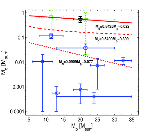
Figure 1: Observational estimates of the masses of newly formed dust M${}_{\textrm{d}}$ in the CCSNæ (four-points stars and solid line error bars) as a function of the progenitor mass M${}_{\textrm{p}}$, both expressed in solar units. The recent estimates of the amount of newly formed dust in Kepler SNa (square with dotted line error bars), Cas A (circle with dotted line error bars) obtained by sub-mm observations, and in SN 1987A (five-pointed star with continuous line error bars) with the PACS/SPIRE onboard the Herschel Space Observatory are also displayed. Three fits are shown: the dotted line represents the best fit obtained from using only the masses of dust determined by NIR/MIR observations; the dashed line represents the best fit to all the data; finally, the continuous line represents the best fit only to the amounts of dust derived from FIR/sub-mm data.

Given these premises, several important questions arise. How much dust is produced by a single SNa according to the observational data ? What is the condensation efficiency of the different refractory elements during the evolution of the SNa remnants (Nozawa et al. 2003; Ercolano et al. 2007; Cherchneff & Lilly 2008; Zhukovska et al. 2008; Calura et al. 2008), in particular when the effects of forward and reverse shocks are taken into account (Nozawa et al. 2006, 2007; Kozasa et al. 2009) ? Do SNæ produce enough dust to significantly contribute to the obscuration of primordial galaxies (Dwek et al. 2007; Nozawa et al. 2008; Dwek & Cherchneff 2011; Gall et al. 2011b) or a substantial amount of that dust is due to nucleation in the ISM with SNæ mainly providing the seeds on which dust grains of the ISM grow (Dwek et al. 2009; Draine 2009; Mattsson 2011) ? Do current theoretical models of dust formation (Todini & Ferrara 2001; Nozawa et al. 2003; Schneider et al. 2004; Kozasa et al. 2009) agree with the observational data (Rho et al. 2008, 2009a; Kozasa et al. 2009; Rho et al. 2009b; Matsuura et al. 2011) ? Finally, which kind of SNæ produce dust? We need to deal with all these questions to build a reliable set of dust yields by SNæ to be included in chemical models of galaxies.
How much dust can a single supernova inject into the ISM ? Since the early observations of the SNa 1987A, this question has long been debated with controversial answers. The reasons of uncertainty can be summarized as follows: (1) The sample of observed SNæ with ongoing dust formation is small (Kozasa et al. 2009) so that it is almost impossible to get some reliable clues about the link between mass and metallicity of the progenitor and the amount of produced dust; (2) The MIR-NIR observations could miss the presence of a significant amount of cold and very cold dust. Only with SCUBA-2, ALMA, and Herschel Space Observatory we might be able to highlight this issue (Gomez et al. 2007; Rho et al. 2008; Nozawa et al. 2008; Dunne et al. 2009; Gomez et al. 2009). The very recent discovery of a significant amount of very cold dust grains in SN 1987A (Matsuura et al. 2011) seems to strengthen this point, thus suggesting that, as suspected, NIR/MIR observations are not able to trace a complete picture of the dust in SNæ; (3) It is not clear if and how much dust is embedded in a thin envelope or in thick clumpy regions (Ercolano et al. 2007), thus making quantitative estimates highly uncertain. In some cases the assumption that the radiation emitted by dust comes from an optically thin region could lead to large errors (Kozasa et al. 2009; Meikle et al. 2007); (4) It is always a cumbersome affair to discriminate between contamination by foreground dust and dust residing and forming locally in the observed SNa (see for instance the discussion on the foreground contamination in the case of CasA by Dunne et al. 2003; Krause et al. 2004; Wilson & Batrla 2005; Rho et al. 2008). What do observations tell us? Till now, ongoing dust formation in the ejecta of thermonuclear type Ia SNæ has not been observed (Kozasa et al. 2009; Draine 2009), even if for instance the classification of the Kepler SNa is still uncertain and perhaps suggesting a type Ia SNa (Gomez et al. 2009). As nowadays, a great deal of the observational evidence of dust formation comes from family of type II SNæ otherwise known as CCSNæ. The Only exceptions in the family of CCSNæ are the type Ic SNæ, in which no dust has been revealed so far (Kozasa et al. 2009).
In Table LABEL:tabella1 we summarize the most significant observations of dust formation in SNæ, together with the available information about the progenitor mass and the SNa type. It is soon evident that, despite the growing number of observed objects and the improved quality of the data with the new IR telescopes, our current knowledge of the problem is still far from being satisfactory. Because of the uncertainties and the poor statistics, it is not possible to disentangle the complex dependence of the observed ongoing dust formation on physical parameters like the mass and metallicity of the progenitor star and the density of the underlying environment where the explosion took place. In Fig. 1 we display the current observational estimates of the amounts of dust together with their uncertainties as a function of the progenitor mass (the entries of Table LABEL:tabella1). For Kepler and Cas A SNæ we plot also the estimates derived from taking into account recent sub-mm determinations of the cold dust contribution (Dunne et al. 2009; Gomez et al. 2009). In the same way, for SN 1987A we plot the new estimate of the dust mass derived from FIR/sub-mm observations with PACS and SPIRE onboard Herschel Space Observatory. Finally, we fit our small and scattered sample of data with simple analytical expressions. If we consider all the objects whose estimates of the dust content is based only upon observations of warm dust in the NIR/MIR, the analytical fit yields about 0.006-0.05 M_⊙ of dust per SNa, depending on the progenitor mass. Clearly, this is only a mean lower limit because we are neglecting the cold dust emitting at longer wavelengths. As suggested by the FIR/sub-mm data for Cas A (Dunne et al. 2009), Kepler (Gomez et al. 2009) and SN 1987A (Matsuura et al. 2011), the contribution by cold dust could easily increase the average estimate by one or even two orders of magnitude, i.e. up to 0.1-0.2 M_⊙ of dust per SNa (dashed line in Fig. 1). If we consider only the observations taking into account FIR/sub-mm data, we get 0.4-0.7 M_⊙ per SNa: in this case SNæ would be very efficient dust factories! However, with a sample of only three data drawing any conclusion would be premature. In any case, the data on the cold wing of the dust population clearly indicates that SNæ are not poor dust producers as claimed by Zhukovska et al. (2008). The issue is anyway still open. Therefore, even ignoring the other points of uncertainty we have mentioned above, i.e. the thin layer approximation, the poor statistics and the foreground contamination, the sole large uncertainty on the contribution by cold dust renders the whole subject highly uncertain. More sub-mm data from SCUBA-2, ALMA, and Herschel Space Observatory are needed to solve the problem.

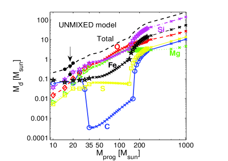
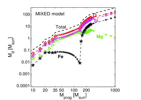
Figure 2: Yields of dust for C, O, Mg, Si, S and Fe, calculated from the list of dust compounds of Nozawa et al. (2003) and the unmixed (Left Panel) and mixed (Right Panel) models of ejecta as a function of the progenitor mass. All quantities on display are expressed in solar masses. Small crosses represent extrapolations from the data of Nozawa et al. (2003) to other mass ranges. The legend is as follows: C (empty circles and continuous line); O (diamonds and dashed line); Mg (triangles and dotted line); Si (six-pointed stars and dot-dashed line); S (squares and continuous line) and Fe (five-pointed stars and dashed line). The dashed line without markers represents the total amount of dust left over by the shocks in the SNR. We also show (filled circles) the total yields of dust by Kozasa et al. (2009) for the unmixed 15, 18 and 20M_⊙ models. The effect of a different hydrogen-rich envelope on the amount of dust formed by a 18M_⊙ model is also indicated by the arrow.

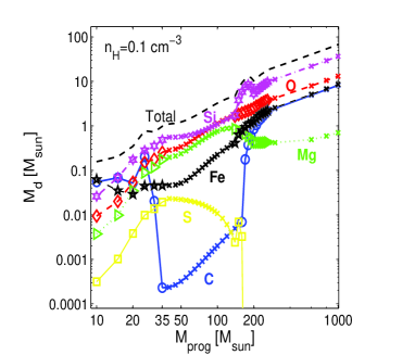
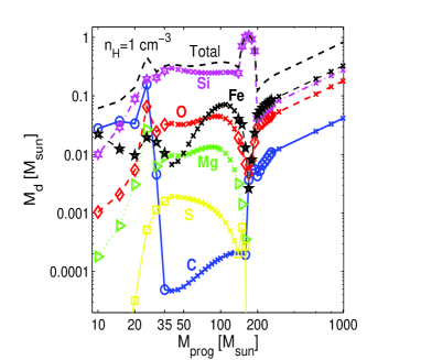
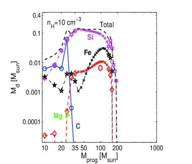
Figure 3: Masses of C, O, Mg, Si, S and Fe, hidden in the dust and left over by the reverse shocks in SNRs (Nozawa et al. 2007) as a function of the progenitor mass, for the unmixed grain model of Nozawa et al. (2003) and at varying the hydrogen number density n${}_{\textrm{H}}$. All quantities on display are expressed in solar masses. Small crosses represent extrapolations from the dust yields calculated by Nozawa et al. (2003) to other mass ranges. The legend is as follows: C (empty circles and continuous line); O (diamonds and dashed line); Mg (triangles and dotted line); Si (six-pointed stars and dot-dashed line); S (squares and continuous line) and Fe (five-pointed stars and dashed line). The dashed line without markers represents the total amount of dust survived to the shocks in the SNR. Left Panel: Masses of C, O, Mg, Si, S and Fe in dust survived to reverse shocks for n${}_{\textrm{H}}=0.1\,$cm^-3. Middle Panel: The same as in left panel but for n${}_{\textrm{H}}=1\,$cm^-3. Right Panel: The same as in left panel but for n${}_{\textrm{H}}=10\,$cm^-3.

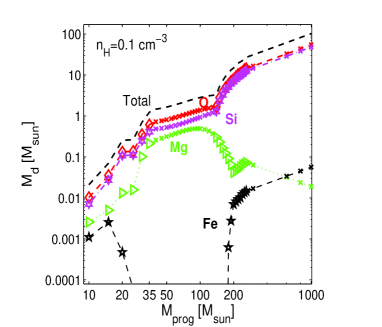
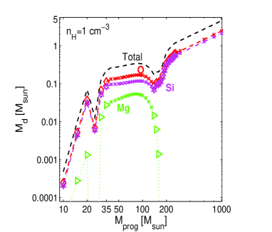
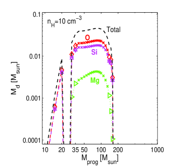
Figure 4: The same as in Fig. 3 but for the mixed grain model by Nozawa et al. (2003). The meaning of all the symbols is the same as in Fig. 3. Left Panel: The masses of O, Mg, Si and Fe in dust that survived to the reverse shocks for n${}_{\textrm{H}}=0.1\,$cm^-3. Middle Panel: The same as in left panel but for n${}_{\textrm{H}}=1\,$cm^-3. Right Panel: The same as in left panel but for n${}_{\textrm{H}}=10\,$cm^-3.

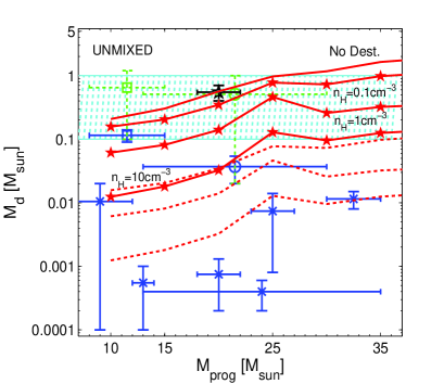
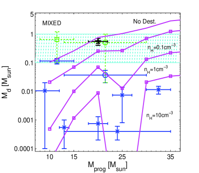
Figure 5: Comparison between theoretical models and observational data. The amount of dust surviving destruction is shown for three ambient number densities n${}_{\textrm{H}}=0.1$ cm^-3, n${}_{\textrm{H}}=1$ cm^-3 and n${}_{\textrm{H}}=10$ cm^-3. Also, the original undestroyed yields by Nozawa et al. (2003) are displayed. The crosses, circles, squares and five-pointed star represent observational data from Table LABEL:tabella1 relative to freshly formed dust in SNRs, as in Fig. 1, with the same meaning of the symbols. The hatched area in both panels represent the amount of dust per SNa needed to explain the obscured high-z quasars, according to the estimates by Dwek et al. (2009). Left panel Theory vs. observation for the unmixed model. The solid line without marks shows the undestroyed yields. The continuous lines from top to bottom show the yields at increasing n${}_{\textrm{H}}$. Dotted lines represent the three n${}_{\textrm{H}}$ re-scaled by a factor of 10. Right panel Theory vs. observation for the mixed model. The continuous lines have the same meaning as in the left panel.

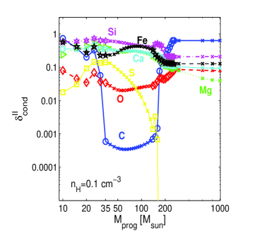
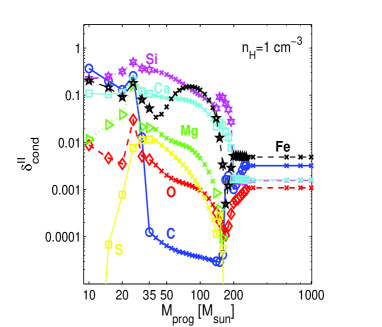
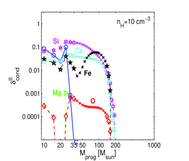
Figure 6: Condensation efficiencies of the elements C, O, Mg, Si, Ca, S and Fe in SNRs as a function of the progenitor mass, according to the unmixed grain models of Nozawa et al. (2003, 2007) and at varying the hydrogen number density n_H. The small crosses represent extrapolations of the yields of dust by Nozawa et al. (2003) to other mass ranges. We plot: C (empty circles and continuous line); O (diamonds and dashed line); Mg (triangles and dotted line); Si (six-pointed stars and dot-dashed line); S (squares and continuous line); Ca (squares and continuous line) and Fe (five-pointed stars and dashed line). Left Panel: Condensation efficiencies of C, O, Mg, Si, S and Fe in dust survived to reverse shocks in a medium with n${}_{\textrm{H}}=0.1\,$cm^-3. Middle Panel: The same as in left panel but for n${}_{\textrm{H}}=1\,$cm^-3. Right Panel: The same as in left panel, only for n${}_{\textrm{H}}=10\,$cm^-3.

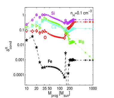
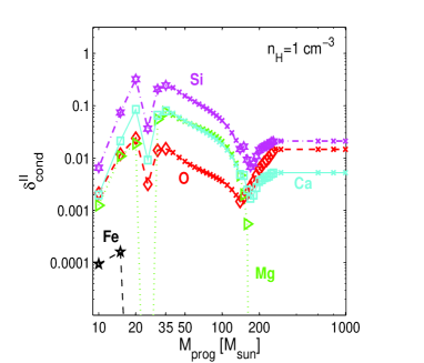
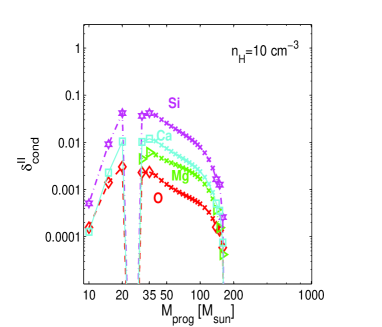
Figure 7: The same as in Fig. 6 but for the mixed grain model of Nozawa et al. (2003, 2007). The meaning of all the symbols is the same as in Fig. 6. Left Panel: Condensation efficiencies of O, Mg, Si, Ca and Fe for n${}_{\textrm{H}}=0.1\,$cm^-3. Middle Panel: The same as in left panel but for n${}_{\textrm{H}}=1\,$cm^-3. Right Panel: The same as in left panel but for n${}_{\textrm{H}}=10\,$cm^-3.

How the empirical data compare with the theoretical models? Until now, an handful of studies have tried to theoretically model dust (Todini & Ferrara 2001; Nozawa et al. 2003; Schneider et al. 2004; Kozasa et al. 2009) and molecules (Cherchneff & Lilly 2008; Cherchneff & Dwek 2009, 2010) formation in SNæ, coupling a more or less refined classical nucleation theory (CNT) or kinetic theory with models of SNæ explosions able to follow for hundred of days the evolution of the expanding envelope. Even if some of these studies have been dedicated to Population III SNæ, their results and conclusions can be applied to SNæ with progenitors of different metallicities, even with super-solar values. Indeed, according to Todini & Ferrara (2001) and Nozawa et al. (2003), dust formation in the ejecta is almost insensitive to the metallicity of the progenitor stars. The processes of dust destruction and cooling in the surrounding ISM are also scarcely dependent on the ISM metallicity (Nozawa et al. 2007, 2008). The most complete compilation of dust yields are, even if limited to Pop III SNæ, by Nozawa et al. (2003). In brief, they modelled the formation of dust in CCSNæ from 13 to 30 M_⊙ and Pair-Instability SNæ (PISNæ) from 170 to 200 M_⊙ for both unmixed and mixed He cores and including a wide range of dust compounds. From their database we derived the mass of each element embedded in the dust components. More details of it are given in Appendix A. In Fig. 2 we show the yields of dust for each element and the total yield, for both unmixed (left panel) and mixed (right panel) cases. Since the progenitor masses in the Nozawa et al. (2003) grid do not cover the whole range of possible values some interpolation/extrapolation of the data have been applied. Owing to the coarse coverage of large mass intervals, the interpolation/extrapolation procedure may be affected by large uncertainties. In general, in the case of unmixed cores, many dusty compounds form, in particular the carbon and sulphur dust, that do not form in the mixed case. In this latter, oxygen atoms are more abundant than carbon atoms and only silicates and oxides form (Nozawa et al. 2008). The general trend of all the elements is quite regular, with just some exceptions, like carbon (in the unmixed model) and iron (in the mixed model): the yields grow at growing mass of the progenitor.
Compared with the observational data, are the theoretical yields satisfactory? Before comparing theory and observations, we have taken into account the dynamical evolution of the dust and its destruction in SNRs, in particular due to the passage of the reverse shock (Nozawa et al. 2007; Bianchi & Schneider 2007). Basing on previous studies by Nozawa et al. (2003) and Nozawa et al. (2006), Nozawa et al. (2007) calculated the dust yields and sizes of dust grains surviving destruction. Starting from the yields described in Appendix A and multiplying them for the destruction coefficients (Nozawa et al. 2007), we derive the new yields as a functions of the ambient numerical density n${}_{\textrm{H}}$ that are presented in Figs. 3 (unmixed model) and 4 (mixed model). Here, we show the amount of each element embedded into dust grains and finally injected into the ISM without being destroyed in the SNR evolution as a function of the ambient gas number density $\textrm{n}_{\textrm{H}}$. In both mixed and unmixed cases, the higher the ambient density $\textrm{n}_{\textrm{H}}$, the higher is the amount of dust destroyed and the smaller the yields. Some elements, like S or Mg in the unmixed case or Fe in the mixed one, are completely destroyed in high density environments.
Finally, in Fig. 5 we compare the theoretical yields with the observational data, for both the unmixed and mixed models. The yields based on the unmixed models marginally agree with the observational data obtained from the MIR observations of SNRs. To get a satisfactory agreement with the MIR estimates of the dust content we would need to re-scale the yields from unmixed models by at least a factor of 10 (see as Fig. 5). However, these yields much better agree with the estimates of the dust content in Kepler, Cas A (dotted crosses) and 1987A (continuous black cross) SNæ , once the contribution by cold dust is included (Gomez et al. 2009; Dunne et al. 2009; Matsuura et al. 2011). These more recent data increase the dust production by SNæ by at least one order of magnitude. In any case, a satisfactory comparison between data and theory, the latter including also accurate evaluations of the amounts of cold dust, would be possible if more and better observations of SNæ in the FIR/sub-mm become available. The yields based on mixed models, because of the stronger destruction of dust grains in the SNRs, better agree with the MIR observations, but considering the contribution of cold dust they fail to match the FIR/sub-mm data unless the SNa explosion takes place in a low density environment.
Condensation efficiencies. Once the original total yields from the SNæ models are known, one can derive the condensation efficiencies of the various elements. One could refer to the study by Nozawa et al. (2003) who used ad-hoc hydrodynamic models and results of nucleosynthesis calculations that were based on the models by Umeda & Nomoto (2002), but with different properties, like the mass-cut, progenitor mass, Y_e and explosion energy (T. Nozawa, private communication). Unfortunately these SNa models are not publicly available. To cope with this, we follow the suggestion by Umeda (2011, private communication) and make use of the up-to-date nucleosynthesis calculations by Nomoto et al. (2006); Tominaga et al. (2007) and the original models by Umeda & Nomoto (2002) to get the final dust-to-gas ratios from the gaseous yields (the correct correspondence between the parameters of the SNa models and those used to derive the yield of Nozawa et al. (2003) is secured).

In Figs. 6 and 7 we show the condensation efficiencies of C, O, Mg, Si, S and Fe for the unmixed model and O, Mg, Si, Ca and Fe for the mixed one, both at varying the ambient density n${}_{\textrm{H}}$. Obviously for the highest densities, more grains are destroyed before being injected into the ISM and therefore the condensation efficiencies are lower. In our chemical model we consider also the evolution of Ca. This element is not considered in the nucleation models by Nozawa et al. (2003), but is included in the SNa yields by Portinari et al. (1998) and with other refractory elements contributes to various pyroxene and olivine minerals. For the condensation efficiency of Ca we adopt the mean value of the other refractory elements (Mg, Si, S and Fe). The result for Ca is shown in Figs. 6 and 7 as a continuous line with empty squares.

How these yields of dust and corresponding condensation efficiencies compare with the amount of dust that is estimated to explain the obscured objects at high redshift? The question is still open and vividly debated, see for instance Dwek et al. (2007, 2009), Draine (2009) and Nozawa et al. (2008), and in particular Maiolino et al. (2004), Wang et al. (2008a, 2009), Wagg et al. (2009) and Michałowski et al. (2010b, a) for high-z observations of obscured quasars and LAEs. It is not clear whether SNæ play a major role as dust producers in high-z, very young galaxies, when AGB stars still have not yet started contributing to the total budget (Sugerman et al. 2006; Bianchi & Schneider 2007; Nozawa et al. 2008), or grain accretion in the ISM dominate leaving to SNRs the role of seed producers over which accretion should take place (Dwek et al. 2009; Draine 2009). Dwek et al. (2009) argue that $0.1-1$M_⊙ of dust is produced by every SNa to fully explain high-z obscured objects, the dust being originating in SNRs. In Fig. 5 we indicate with the hatched area the $0.1-1$M_⊙ region. Our theoretical yields agree with the values falling into the hatched region, in particular for the unmixed case. They may differ by about one order of magnitude from the MIR estimates which, as shown in Fig. 1, indicate about $0.01\,\textrm{M}_{\odot}$ of dust per SNa. Because of it, Dwek et al. (2009); Draine (2009) favoured the accretion in the ISM as the dominant source of dust in high-z quasars. However, more detailed observations of cold dust in some SNRs (Gomez et al. 2009; Dunne et al. 2009), and in particular the recent Matsuura et al. (2011) estimate, significantly increase the dust contribution by SNæ, that becomes high enough to overwhelm the ISM accretion in the early stages. This is also what is theoretically predicted and modelled in the high SFR inner regions of the MW Disk by Piovan et al. (2011b, c). The dust accretion in the ISM requires that some enrichment in metals has already occurred so that some delay is unavoidable. For very high SFR such as in QSOs, the delay can be very short (Gall et al. 2011a, b), thus further complicating the whole picture. The issue is still debated.
Which kind of SNæ produce dust? From the entries of Table LABEL:tabella1 we note that nearly all SNa types are dust producers. The only exception are type Ia SNæ in which no dust has been detected (Borkowski et al. 2006; Draine 2009). In addition to this, in meteorites no pre-solar grains formed in type Ia thermonuclear SNæ explosions have been found (Clayton & Nittler 2004). Therefore, it is most likely that type Ia SNæ have almost zero condensation efficiency. Recently, Kozasa et al. (2009) calculated some models of dust formation in CCSNæ, based upon the same formalism of Nozawa et al. (2003), but using different underlying models of SNæ. The aim was to investigate the effects on dust nucleation of a different amount of hydrogen in the envelope at the onset of the collapse. In Fig. 2 (left panel) we show the total yields of dust by Kozasa et al. (2009) for their unmixed 15, 18 and 20M_⊙ models (filled circles), and compare them with the Nozawa et al. (2003) yields. When the hydrogen-rich envelope at the onset of the collapse is thick, the models agree each other, and the total amount of dust produced is about the same. On the contrary, as indicated by the arrow in Fig. 2 for the 18M_⊙ star, the effect of the hydrogen-rich envelope on the amount of dust produced is significant: for type IIb SNæ it drops by a factor of about three, from $\thicksim$0.45M_⊙ to 0.167M_⊙. This finding for the 18M_⊙ model suggests that in chemical models of galaxies it would be interesting to distinguish the contribution by different types of CCSNæ, e.g. because of different mass loss histories a different onion-like structures of the progenitor (Kozasa et al. 2009; Gall et al. 2011a). The effect of the varying hydrogen envelope could modify our view of the types of SNæ able to produce significant amounts of dust.

Mixed or unmixed. Which is more consistent with observations? Basing on observations of the Cas A remnant (Ennis et al. 2006), Kozasa et al. (2009) prefer to use unmixed models. Furthermore: (i) the unmixed model better reproduces the extinction curves observed in high-z quasars Hirashita et al. (2005); (ii) they are exactly in the range suggested by Dwek et al. (2009) to cope with the high-z obscured universe and, finally, (iii) SNæ have to produce some amount of carbonaceous grains according to observations of pre-solar dust, whereas the mixed model is not able to produce C-based dust. It seems therefore that the unmixed model condensation efficiencies should be preferred. We will present in our tables only the condensation efficiencies for the unmixed case.

Other condensation efficiencies. For the sake of comparison and completeness, we take into account other prescriptions for the efficiency of dust condensation in SNRs. First of all the simple formulation by Dwek (1998) and Calura et al. (2008) who for type II SNæ adopt a set of condensation efficiencies independent from the mass/metallicity of the star or the density of the parental environment:

$$M_{D,A}\left(M,Z\right)=\delta^{II}_{c}\left(A\right)M_{A}\left(M,Z\right)$$ (1)

$$M_{D,C}\left(M,Z\right)=\delta^{II}_{c}\left(C\right)M_{C}\left(M,Z\right)$$ (2)

where $M_{A}\left(M,Z\right)$ is the mass of the generic element $A$ ejected by the star of mass $M$ and metallicity $Z$, and A$=$ Mg, Si, S, Ca, Fe (all the refractory elements included into the model), but carbon. $M_{C}\left(M,Z\right)$ is the ejected mass of carbon. $\delta^{II}_{c}\left(C\right)$ and $\delta^{II}_{c}\left(A\right)$ are the condensation efficiencies of Carbon and refractory elements, finally $M_{D,C}\left(M,Z\right)$ and $M_{D,A}\left(M,Z\right)$ are the ejected mass of dust for carbon and element $A$. For the oxygen an average between the refractory elements is used, where every element is weighted for its mass number $\mathcal{A}_{A}$:

$$M_{D,O}\left(M,Z\right)=16\sum_{A}\delta^{II}_{c}\left(A\right)\frac{M_{A}\left(M,Z\right)}{\mathcal{A}_{A}}$$ (3)

where A=Mg,Si,S,Ca,Fe. A similar set of equation is used for type Ia SNæ with the condensation factors indicated by $\delta^{I}_{c}$. The adopted values are $\delta^{II}_{c}\left(A\right)=\delta^{I}_{c}\left(A\right)=0.8$ for $A={Mg,Si,S,Ca,Fe}$ and $\delta^{II}_{c}\left(A\right)=\delta^{I}_{c}\left(A\right)=0.5$ for C. No distinction is made for the condensation efficiencies between type II CCSNæ and thermonuclear type Ia SNæ. The values for the condensation efficiencies are somewhat arbitrary (Dwek 1998); they are simply meant to indicate the effect of condensation with some destruction. One of the most controversial issues is the assumption made by Dwek (1998) and Calura et al. (2008) about Type Ia SNæ: the condensation efficiencies are assumed to be high despite the fact that no dust formation has been observed in Type Ia SNRs (Draine 2009). This contradictory assumption has been recently corrected in Pipino et al. (2011). Calura et al. (2008) also assume condensation efficiencies all equal to 0.1 and compare the results with those of Dwek (1998). They find that the fraction of newly formed dust is nearly independent from the condensation efficiencies if dust accretion and destruction balance each other as it seems to be the case of the MW at the present age (Dwek 1998; Zhukovska et al. 2008). However, this could not be true for different ages in the history of MW or for other galaxies with different SFHs. Finally, the destruction-accretion balance may heavily depend on subtle details of the two processes and their uncertainties errors. For all these considerations, we suggest that the more detailed set of condensation efficiencies based on Nozawa et al. (2003, 2006, 2007) that we analyzed above, is more safe and of general use to be adopted into theoretical models. It relies on detailed models that are still the most handy available in literature thanks to the number of modelled masses, to the included effects of the reverse shock and environmental density on the surviving mass of dust grains.
However, we are still far away from a satisfactory picture. Indeed, an important point to consider is that the classical nucleation theory (CNT), widely used to model the formation of dust in SNæ, has been improperly applied. The founding hypotheses of this theory do not hold in the SNæ environment, that is neither at equilibrium nor at steady state. As recently shown by Cherchneff & Lilly (2008), Cherchneff & Dwek (2009); Cherchneff (2009), and (Cherchneff & Dwek 2010), the steady state is not reached, complicating the problem since molecules would act as a bottleneck against dust formation (Nozawa et al. 2008). Molecules affect dust formation by depleting the gas from metals and cooling the environment. A kinetically driven approach should be therefore used and the formation of molecules, as dust precursors, should be properly treated, thus influencing the nucleation models for dust formation in SNæ. As shown by Cherchneff & Dwek (2010), a proper stochastic, kinetic approach leads to masses of dust that can be 2-5 times less than the amount predicted by Nozawa et al. (2003). Interestingly, this reduction in the dust mass would produce a worst agreement between the observational data in Fig. 5 and the predictions of the unmixed model. Furthermore, as outlined by (Cherchneff & Dwek 2010), the dust mixture produced with the kinetic description is different. Standing on these considerations, it is clear that detailed databases of dust yields by SNæ, taking into account different progenitor masses and metallicities, hydrogen envelopes and molecules formation, are needed. Doing this would greatly improve upon the equilibrium and steady state approximation. Nevertheless, as long as models at varying those parameters are not available, the current estimates of the condensation efficiencies by Nozawa et al. (2003, 2006, 2007) can be safely used in chemical models.
Another prescription for dust condensation in SNæ worth being examined is the one by Zhukovska et al. (2008). They assume that SNæ are poor producers of dust. This hypothesis is likely contradicted by the recent estimates of dust content in Cas A, Kepler SNa, and SN 1987A. Anyway, according to Zhukovska et al. (2008), the uncertainties on dust formation in SNæ are still so large that purely theoretical yields cannot be safely used. Therefore, they adopt the same scheme of Dwek (1998), introduce condensation factors independent from both mass of the progenitor and/or metallicity, and assume that Type II SNæ produce all types of dust, while Type Ia produce only small amounts of iron.
To adapt their scheme and use it into our model (see below Sect. 4 and Piovan et al. 2011b, for more details about the chemical model), we must switch from their description limited to some typical dust grains as a whole to ours in which single elements are followed both in gas and dust and as a whole in the ISM. Let $M_{i,j}\left(M,Z\right)$ be the ejecta for the key-element $i$-th of the $j$-type of grain (Zhukovska et al. 2008), coming from a SNa of mass $M$ and metallicity $Z$. If we divide by the mass of the key-element $A_{i,j}m_{H}$ we get the number of atoms of the key-element $i$-th available for dust formation. Dividing again by the number of atoms of the key-element $\nu_{i,j}$ for one unit of dust $j$ (we can simply assume $\nu_{i,j}=1$) and multiplying by the mass of one grain we get the maximum mass of dust that can be formed. A multiplicative factor can be the introduced to take into account the higher or lower efficiency of the condensation process

$$M_{D,j}\left(M,Z\right)=\delta_{c,j}^{Ia,II}\cdot\frac{A_{j,d}}{A_{i,j}}\cdot M_{i,j}\left(M,Z\right)$$ (4)

where $i$ refers to the key-element and $j$ to the type of dust grain. The ejecta is simply scaled by means of the ratio between the atomic weights and multiplied for the condensation factor to get the $j$-th type of dust injected into the ISM. If we want the amount of the element $k$-th ejected in form of dust we have:

$$M_{D,k}\left(M,Z\right) =\sum_{j=1}^{n}M_{D,j}\left(M,Z\right)\frac{A_{k,j}}{A_{j,d}}=$$

$$=\sum_{j=1}^{n}\delta_{c,j}^{Ia,II}\cdot\frac{A_{k,j}}{A_{i,j}}\cdot M_{i,j}\left(M,Z\right)$$ (5)

where $A_{k,j}=A_{i,j}$ if the element of interest coincides with the key element. The condensation factors in use here are much lower than for instance those of Dwek (1998); Calura et al. (2008): $\delta_{c,j}^{II}$ is 0.00035, 0.15, 0.001, 0.0003 respectively for silicates, carbonaceous grains, SiC and iron grains, while $\delta_{c,j}^{Ia}$ is always zero except for iron where it is 0.005 (in order to agree with the observations). In particular, the dust condensation efficiencies for the refractory elements involved in the formation of silicates are very low. Indeed, they are calibrated on the observational hints from meteorites and interplanetary dust particles, where the number of detected silicates is small up to now. According to Zhukovska et al. (2008), these low values could be also explained if we take into account all the local destructive processes affecting the SNa grains in the ISM (mostly the reverse shock and also shocks inside the star cluster itself).

3 Yields of dust from AGB stars

While SNRs from massive stars eject newly formed dust in amounts that are largely uncertain, low and intermediate mass stars in the asymptotic giant branch (AGB) phase are long known to safely be strong injectors of dust in the ISM. It is worth noting that previous evolutionary phases of low and intermediate mass-stars are not so important: dust formation in the red giant branch (RGB) and even early asymptotic giant branch (E-AGB) stars can be ignored because the physical properties of their stellar winds do not favour dust formation and the rates of mass loss are very low (Gail et al. 2009). Only the thermally pulsing AGB (TP-AGB) stars are expected to form dust in significant amounts.
TP-AGB stars have been the subject of an impressive number of studies based on the theory of stellar evolution and going from synthetic models (see for instance Groenewegen & de Jong 1993; Marigo et al. 1996; Wagenhuber & Groenewegen 1998; Marigo 2002; Izzard & Poelarends 2006; Marigo & Girardi 2007) to full calculations of evolutionary, even hydrodynamical, models (see for instance Herwig et al. 1997; Karakas et al. 2002; Ventura et al. 2002; Herwig 2004; Weiss & Ferguson 2009). Moreover, dust formation in AGB stars has been the subject of more and more refined and detailed models (Gail et al. 1984; Gail & Sedlmayr 1985, 1987; Dominik et al. 1993; Gail & Sedlmayr 1999; Ferrarotti & Gail 2002, 2006; Gail et al. 2009), able to calculate the amount of newly formed dust in M-stars, S-stars and C-stars, along a sequence of growing C/O ratio. This ratio determines the dust mixtures formed in the outflows (Piovan et al. 2003; Ferrarotti & Gail 2006; Gail et al. 2009). AGB stars with C/O$<$1 are oxygen-rich stars, that produce dust grains mainly formed by refractory elements, generically defined as silicates, like pyroxenes and olivines, oxides like alumina and maybe iron dust. When the C/O ratio is higher than one, we have carbon-rich stars in outflows of which carbon dust, SiC, and even iron dust can condensate. SiC is detected by means of the typical MIR feature. When C/O $\approx$ 1 then we get S-stars where quartz and iron dust should form (Ferrarotti & Gail 2002). However the C-rich or O-rich phases dominate, so that for example the contribution of SiC produced during the S phase can be neglected compared to the SiC produced during the carbon-star phase.
Depending on the initial mass, the metallicity and the complex interplay between the third dredge-up and mass-loss, the star will become or not carbon-rich. Typically, low mass stars are not able to become C-rich, because they loose the envelope before that carbon overcomes the oxygen abundance, while intermediate mass stars are able to reach C/O$>$1, even if in some cases only for a short part of the TP-AGB (as it happens for the most massive AGB stars). Recently, Ferrarotti & Gail (2006) presented a detailed database of dust yields from AGB stars, where many compounds are taken into account. This database has been later extended by Zhukovska et al. (2008). Even if, as pointed out by Draine (2009), the dust yields from AGB stars are not known at the same level of confidence as the purely gaseous ones, they are surely much better known than those from SNæ ejecta.
Ferrarotti & Gail (2006) models are obtained applying the schemes for dust formation to synthetic AGB models standing on Groenewegen & de Jong (1993) and Marigo et al. (1996). Similar recipes have been proposed by van den Hoek & Groenewegen (1997) and have been adopted as reference scheme for the total gaseous yields (see Zhukovska et al. 2008, for more details). Also, for some elements the results by Karakas & Lattanzio (2003) have been used. Since we want to obtain the dust condensation coefficients $\delta_{c,i}^{w}$ for every element $i$-th of our set, first of all we must calculate the amount of each element embedded in newly formed dust. The details of these calculations are given Appendix Appendix B.

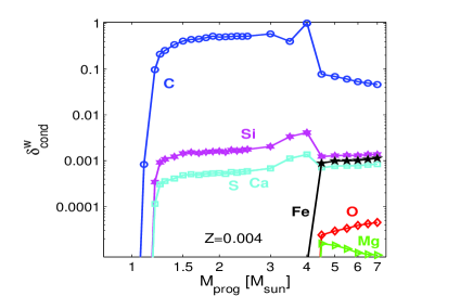
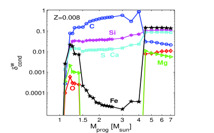
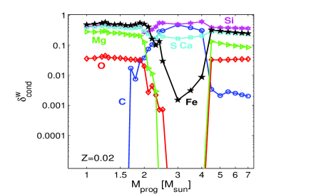
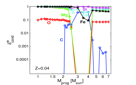
Figure 8: Condensation efficiencies for the elements C, O, Mg, Si, Ca, S and Fe in SNRs as a function of the progenitor mass at varying the metallicity Z. We plot: C (empty circles and continuous line); O (diamonds and dashed line); Mg (triangles and dotted line); Si (six-pointed stars and dot-dashed line); S and Ca (squares and continuous line) and Fe (five-pointed stars and dashed line).

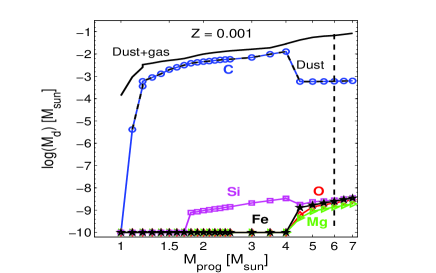
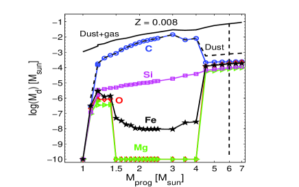
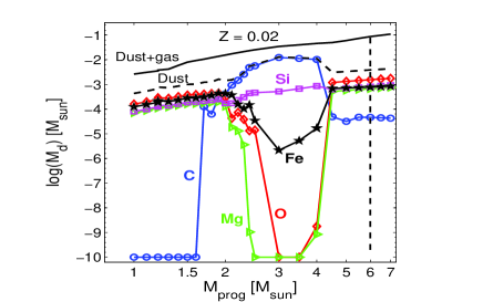
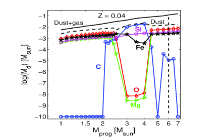
Figure 9: Dust ejecta for C, O, Mg, Si, and Fe, calculated by means of dust compounds of Ferrarotti & Gail (2006); Zhukovska et al. (2008) for AGB stars as a function of the progenitor mass. Four metallicities are considered. The legend is as follows: C (empty circles and continuous line); O (diamonds and dashed line); Mg (triangles and dotted line); Si (six-pointed stars and dot-dashed line); S (squares and continuous line) and Fe (five-pointed stars and dashed line). The dashed line without markers is the total amount of dust in the ejecta. The vertical dashed line represents the 6 M_⊙ upper AGB limit according to our set of yields Marigo et al. (1996, 1998); Portinari et al. (1998). Finally, the continuous line shows the total ejected mass in dust and gas for what concerns the five elements we have considered in the plot according to van den Hoek & Groenewegen (1997).

In Fig. 9, for the elements C, O, Mg, Si, Fe, we show the total amount $M_{i,d}\left(M,Z\right)$ of dust formed in the outflows of AGB stars, according to the models by van den Hoek & Groenewegen (1997); Ferrarotti & Gail (2006); Zhukovska et al. (2008). Moreover, for each AGB star, we show the total amount of ejected dust and compare it to the total amount of lost material. The following remarks can be made. First, as shown in the top panels, the dust produced by low metallicity AGB stars of any mass is carbon dominated. This point seems to agree with the suggested high-z scenario in which the appearance of the PAH features and graphite extinction bump in the UV are both connected to the delayed injection of carbon by AGB stars, as shown by observations of galaxies of different metallicity (Dwek 2005; Galliano et al. 2008; Dwek et al. 2009). In the early universe, before the most massive AGB stars start contributing to the dust content of the ISM, only SNæ are injecting dust. It is worth noticing that this scenario, based upon the dust production by different stellar sources, needs deeper investigations. The works by Dwek et al. (2009) and Draine (2009) have shown that a significant amount of dust should be produced also by accretion in the ISM (therefore dust would not be only of stellar origin). In the extreme case, the role played by SNæ could be even limited to only injecting metals and seeds for grain growth. However, the recent observations of large amounts of cold dust in SNæ (Dunne et al. 2009; Gomez et al. 2009; Matsuura et al. 2011) reshuffled the problem putting again SNæ on the table as possible major dust factories. Second, at growing metallicity, silicate dust starts to be formed in significant amount, however there is always some injection of carbon dust from stars around 3M_⊙. Third, the following questions arise: At which mass do AGB stars disappear? What is the role played by Super-AGB (SAGB) stars (if any)? Is there any mass range for the existence of thermonuclear SNæ from single stars igniting carbon? What is the lower mass limit for core collapse SNæ (CCSNæ)? Our recipe is strictly classical and follows the one adopted by Portinari et al. (1998) to calculate the chemical yields, since we will base our simulations upon the latest release of those yields. Below 6 solar masses we have stars ending as WDs through the AGB channel; for masses between 6 and 8M_⊙ Portinari et al. (1998) assumed 1.3M$\odot$ of remnant, either WD or NS, and the overlying layers expelled either by an explosion or a TP-AGB phase; for masses M$>8$M_⊙ we have stars developing an iron core and exploding as CCSNæ. However, other mass limits would be possible considering all the uncertainties affecting the evolution of stars in the mass range 6 to 12M_⊙. For instance Zhukovska et al. (2008) and Gail et al. (2009) extend the AGB stars to stars with initial mass of 8M_⊙ and neglect the possibility of SAGB stars; Calura et al. (2008) assume also quiescent outflows until 8M_⊙. Although the investigation of this point is beyond the aims of this study, it is worth keeping in mind that stellar models in this particular mass range are still far from being fully understood, and therefore different mixtures of dust could be formed and ejected.

Once the masses of dust ejecta $M_{i,d}\left(M,Z\right)$ are defined, we can obtain the condensation efficiencies for the element $i$-th during the TP-AGB phase as:

$$\delta_{i}^{w}=\frac{M_{i,d}\left(M,Z\right)}{\Delta M^{AGB}\left(M,Z\right)\cdot X_{i,0}\left(M,Z\right)+M\cdot p_{i}\left(M,Z\right)}$$ (6)

where $\Delta M^{AGB}\left(M,Z\right)\cdot X_{i,0}\left(M,Z\right)$ is the mass of the $i$-th element ejected according to the initial abundance of that element in the stellar model and $M\cdot p_{i}\left(M,Z\right)$ is the newly formed and ejected amount of the same element. In Fig. 8 we show the condensation efficiencies at growing metallicity. While the condensation efficiency of carbon keeps quite high, for oxygen and other refractory elements it grows at increasing metallicity. For metallicity two times solar, for some elements like Si and some stellar masses, almost all the material is condensed into dust. For the sake of comparison we consider also another possibility for the condensation efficiencies, widely adopted in literature, and proposed by Dwek (1998) for AGB stars. They depend on the final C/O ratio in the ejecta, without following the evolution of the star along the AGB as in the complex dust nucleation model by Ferrarotti & Gail (2006) and they are also independent from the metallicity of the stars. If C/O$>$1 then:

$$M_{D}\left(C,M\right)=\delta^{w}_{c}\left(C\right)\left[M_{ej}\left(C,M\right)-\frac{3}{4}M_{ej}\left(O,M\right)\right]$$ (7)

$$M_{D}\left(A,M\right)=\delta^{w}_{c}\left(A\right)\cdot M_{ej}\left(A,M\right)=0$$ (8)

where $M_{D}\left(C,M\right)$ and $M_{D}\left(A,M\right)$ are the ejected masses of C and the generic refractory element $A$ embedded into dust; $M_{ej}\left(C,M\right)$, $M_{ej}\left(O,M\right)$ and $M_{ej}\left(A,M\right)$ are the ejected masses of carbon, oxygen and refractory element $A$ from the star of mass $M$. In our case, $\textrm{A}=\,\textrm{O},\,\textrm{Mg},\,\textrm{Si},\,\textrm{S},\,\textrm{Ca},\,\textrm{Fe}$. $M_{ej}\left(C,M\right)$ is the ejected mass of $C$. $\delta^{w}_{c}\left(C\right)$ and $\delta^{w}_{c}\left(A\right)=0$ are the condensation efficiencies of C and refractory elements. When instead C/O$<$1 then:

$$M_{D}\left(C,M\right)=\delta^{w}_{c}\left(C\right)\cdot M_{ej}\left(C,M\right)=0$$ (9)

$$M_{D}\left(A,M\right)=\delta^{w}_{c}\left(A\right)M_{ej}\left(A,M\right)$$ (10)

$$M_{D}\left(O,M\right)=16\sum_{A}\delta^{w}_{c}\left(A\right)\frac{M_{ej}\left(A,M\right)}{\mathcal{A}_{A}}$$ (11)

where A=Mg,Si,S,Ca,Fe. For the oxygen, the average value of the refractory elements is introduced, where each element is weighted by its mass number $\mathcal{A}_{A}$. In practice $\delta^{w}_{c}\left(A\right)=1$ is chosen, assuming complete condensation of the element.

4 The effect of different yields of dust

We analyzed the most popular recipes adopted in literature to describe the condensation efficiency of dust in the two main dust factories, AGB and SNæ, thus deriving theoretical sets of condensation efficiencies for single refractory elements that can be generally applied to any set of stellar yields. We want now to test these different recipes in a full dust formation and evolution model. At this purpose we introduced the various possibilities for dust condensation efficiencies into the model by Piovan et al. (2011b, c). This model stands on the classical formulation for the chemical enrichment of a galaxy (Chiosi 1980), in his latest multi-ring formulation by Portinari & Chiosi (2000) and Portinari et al. (2004) for disk galaxies, with the introduction of radial flows of matter and galactic bar. The adopted stellar yields are the original ones by Portinari et al. (1998) in its latest revised version (Portinari 2006 - private communication). The model is able to describe the evolution of the abundances of the different refractory elements into dust, properly simulating the process of injection of the stardust into the ISM and the accretion/destruction processes to which the dust is subjected. We trace the evolution of the abundance of both some main typical grain families usually adopted for a general description of a dusty ISM and the single elements into dust.
The complete description of the equations governing the model can be found in Piovan et al. (2011b, c). In the following we briefly introduce only the the equations governing the evolution of the dust component. The evolution of the generic elemental species $i$-th in the dust at the radial distance $r_{k}$ from the centre of the galaxy and at the time $t$, is described according to the extension by Dwek (1998) of the formulation for gas only to a two-component ISM made by gas and dust. Let $\sigma(r,t)$ be the total surface mass density (gas, dust and stars) of the galaxy at the radial distance $r$ and time $t$, and $\sigma(r,t_{G})$ the same but at the galactic age $t_{G}$. The fractionary surface mass density of dust $D(r,t)$ and of the generic element $i$ in form of dust $D_{i}(r,t)$ are given by the following relations

$$D\left(r_{k},t\right)=\frac{\sigma^{D}\left(r_{k},t\right)}{\sigma\left(r_{k},t_{G}\right)}$$ (12)

and

$$D_{i}\left(r_{k},t\right)=\frac{\chi_{i}^{D}\left(r_{k},t\right)\sigma_{D}\left(r_{k},t\right)}{\sigma\left(r_{k},t_{G}\right)}=\chi_{i}^{D}\left(r_{k},t\right)D\left(r_{k},t\right)$$ (13)

where $\chi_{i}^{D}(r,t)$ is the fractionary mass abundance of the element $i$ trapped in the dust, and all surface mass densities are normalized to $\sigma(r,t_{G})$. Identical expressions can be written for the gas component and the corresponding mass abundance of the generic element $i$ trapped in the gas is $\chi_{i}^{G}(r,t)$. By definition the following companion relationship applies $\sum_{i}\left[\chi_{i}^{D}\left(r_{k},t\right)+\chi_{i}^{G}\left(r_{k},t\right)\right]=1$, from which $\sum_{i}\chi_{i}^{D}\left(r_{k},t\right)\neq 1$ and $\sum_{i}\chi_{i}^{G}\left(r_{k},t\right)\neq 1$. Finally, the equations governing the temporal variation of $D_{i}(r,t)$ is

$$\frac{d}{dt} D_{i}\left(r_{k},t\right)=-\chi_{i}^{D}\psi+$$

$$+\int_{0}^{t-\tau_{M_{B,l}}}\psi\left[\phi\delta^{w}_{c,i}R_{i}\cdot\left(-\frac{dM}{d\tau_{M}}\right)\right]_{M\left(\tau\right)}dt^{\prime}+$$

$$+\left(1-A\right)\int_{t-\tau_{M_{B,l}}}^{t-\tau_{M_{SN{\ae}}}}\psi\left[\phi\delta^{w}_{c,i}R_{i}\cdot\left(-\frac{dM}{d\tau_{M}}\right)\right]_{M\left(\tau\right)}dt^{\prime}+$$

$$+\left(1-A\right)\int_{t-\tau_{M_{SN{\ae}}}}^{t-\tau_{M_{B,u}}}\psi\left[\phi\delta^{II}_{c,i}R_{i}\cdot\left(-\frac{dM}{d\tau_{M}}\right)\right]_{M\left(\tau\right)}dt^{\prime}+$$

$$+\int_{t-\tau_{M_{B,u}}}^{t-\tau_{M_{u}}}\psi\left[\phi\delta^{II}_{c,i}R_{i}\cdot\left(-\frac{dM}{d\tau_{M}}\right)\right]_{M\left(\tau\right)}dt^{\prime}+$$

$$+A\int_{t-\tau_{M_{SN{\ae}}}}^{t-\tau_{M_{1},max}}\psi\left[\textit{f}\left(M_{1}\right)\delta^{II}_{c,i}R_{i,1}\cdot\left(-\frac{dM_{1}}{d\tau_{M_{1}}}\right)\right]_{M\left(\tau\right)}dt^{\prime}+$$

$$+A\int_{t-\tau_{M_{1},min}}^{t-\tau_{M_{SN{\ae}}}}\psi\left[\textit{f}\left(M_{1}\right)\delta^{w}_{c,i}R_{i,1}\cdot\left(-\frac{dM_{1}}{d\tau_{M_{1}}}\right)\right]_{M\left(\tau\right)}dt^{\prime}+$$

$$+R_{SNI}E_{SNI,i}\delta^{I}_{c,i}+$$

$$-\left[\frac{d}{dt}D_{i}\left(r_{k},t\right)\right]_{out}+\left[\frac{d}{dt}D_{i}\left(r_{k},t\right)\right]_{rf}+$$

$$+\left[\frac{d}{dt}D_{i}\left(r_{k},t\right)\right]_{accr}-\left[\frac{d}{dt}D_{i}\left(r_{k},t\right)\right]_{SN}$$ (14)

where $\psi(r,t)$ is the star formation rate and $\phi=\phi(M)$ the initial mass function (IMF). The first term at the r.h.s. of eqn. (4) is the depletion of dust because of the star formation that consumes both gas and dust (assumed uniformly mixed in the ISM). The second term is the contribution by stellar winds from low mass stars to the enrichment of the $i$-th component of the dust. Respect to the classical gas-only formulation, the so-called condensation coefficients $\delta^{w}_{c,i}$ determines the fraction of material in stellar winds that goes into dust with respect to that in gas (local condensation of dust in the stellar outflow of low-intermediate mass stars). For these coefficients we can adopt the recipes presented in Sect. 3. The third term is the contribution by stars not belonging to binary systems and not going into type II SNæ (the same coefficients $\delta^{w}_{c,i}$ are used). The fourth term is the contribution by stars not belonging to binary systems, but going into type II SNæ. The condensation efficiency in the ejecta of type II SNæ are named as $\delta^{II}_{c,i}$. For these efficiencies the recipes analyzed in Sect. 2 will be adopted. The fifth term is the contribution of massive stars going into type II SNæ. The sixth and seventh term represent the contribution by the primary star of a binary system, distinguishing between those becoming type II SNæ from those failing this stage and using in each situation the correct coefficients. The eighth term is the contribution of type Ia SNæ, where the condensation coefficients are named as $\delta^{I}_{c,i}$ to describe the mass fraction of the ejecta going into dust. The last four terms describe: (1) the outflow of dust due to galactic winds (in the case of disk galaxies this term can be set to zero); (2) the radial flows of matter between contiguous shells; (3) the accretion term describing the accretion of grain onto bigger particles in cold clouds; (4) the destruction term taking into account the effect of the shocks of SNæ on grains, obviously giving a negative contribution. The infall term in the case of dust can be neglected because we can assume that the primordial material entering the galaxy is made by gas only without a solid dust component mixed to it.
In the model by Piovan et al. (2011b), many choices for the various terms of the eqns. (4) related to dust have been considered and tested together with other prescriptions that are needed to solve the companion equations for gas and total ISM (See Piovan et al. 2011b, for the systems of equations describing the evolution of the gas and ISM). In Table LABEL:Parameters we summarize the list of assumptions/parameters specifying a given model. A detailed description of each possible combination of the parameters is in Piovan et al. (2011b). Let us shortly describe here the parameters in use:

• The IMF determines the relative number of AGB stars, SNæ, and very low mass stars (not contributing to the enrichment of the ISM), thus driving the amounts of star-dust injected by the different sources above. Many IMFs are possible. They are examined in detail by Piovan et al. (2011b). For the purposes of this paper, to analyze the effect of different condensation efficiencies, we consider the IMF by Kroupa (2007) (here indicated by $\mathcal{G}$ according to our identification code). The IMF is kept constant throughout this paper.

• Several laws of star formation can be found in literature (see Piovan et al. 2011b,   for more details). We choose here the star formation law by Dopita & Ryder (1994) (indicated by $\mathcal{D}$) with an intrinsic efficiency given by $\nu=0.55$ (see Piovan et al. 2011b,   for all details). In this study, the law of star formation is kept constant.

• Dust accretion in the cold regions of the ISM strongly depends on the fraction of molecular clouds (MCs) with respect to the gas mass of the ISM. this fraction is named here $\chi_{MC}$. This fraction can be kept constant or varied in time and space. For this latter case, (Piovan et al. 2011c) develop a simple model based on Artificial Neural Networks (ANN) and observational data on the SFR, content of molecular hydrogen H₂, and total gas mass in the SN and MW Disk. With the aid of the ANN we derive from the local values of the SFR and gas mass, the corresponding H₂ mass and it is the one adopted here (case $\mathcal{A}$).

• Two models for the dust accretion in the ISM are available. Here we adopt the most complex one (case $\mathcal{B}$), based upon the work by Zhukovska et al. (2008) and taking into account the numerical densities in the ISM (thus allowing variable time-scales of accretion), the lifetime and the mass of MCs as cold regions where the accretion happens and, finally, a set of dust grains representative of the ISM.

• The condensation efficiencies of type II SNæ, type Ia SNæ and AGB stars are the target of this paper and will be varied and discussed below.

• The galactic bar and the radial flows mechanism of matter exchange between contiguous shells is fixed according to the considerations and models by (Portinari & Chiosi 2000).

Table 3: Parameters of the models. Column (1) is the parameter number, column (2) the associated physical quantity, and column (3) the source and the italic symbols are the identification code we have adopted. See the text for some more details and Piovan et al. (2011b) for a detailed description.

no	Parameter	Source and identification label
1	IMF	Salpeter1 $(\mathcal{A})$, Larson2 $(\mathcal{B}$), Kennicutt3 $(\mathcal{C})$ Kroupa orig.4 $(\mathcal{D})$,
		Chabrier5 $(\mathcal{E})$, Arimoto6 $(\mathcal{F})$, Kroupa 20077 $(\mathcal{G})$, Scalo8 $(\mathcal{H})$, Larson SN9 $(\mathcal{I})$
2	SFR law	Constant SFR $(\mathcal{A})$, Schmidt10 $(\mathcal{B})$, Talbot & Arnett11 $(\mathcal{C})$, Dopita & Ryder12 $(\mathcal{D})$, Wyse & Silk13 $(\mathcal{E})$
3	$\chi_{MC}$ model	Artificial Neural Networks model14 $(\mathcal{A})$, Constant $\chi_{MC}$ as in the Solar Neigh.15 $(\mathcal{B})$
4	Accr. model	Modified Dwek (1998) and Calura et al. (2008) $(\mathcal{A})$; adapted Zhukovska et al. (2008) model $(\mathcal{B})$
5	SNæ Ia model	Dust injection adapted from: Dwek (1998), Calura et al. (2008) $(\mathcal{A})$, Zhukovska et al. (2008) $(\mathcal{B})$
6	SNæ II model	Dust injection adapted from: Dwek (1998) $(\mathcal{A})$, Zhukovska et al. (2008) $(\mathcal{B})$,
		Nozawa et al. (2003, 2006, 2007) $(\mathcal{C})$
7	AGB model	Dust injection adapted from: Dwek (1998) $(\mathcal{A})$, Ferrarotti & Gail (2006) $(\mathcal{B})$
8	Galactic Bar16	No onset $(\mathcal{A})$, onset at $t_{G}-4$ Gyr $(\mathcal{B})$, onset at $t_{G}-1$ Gyr $(\mathcal{C})$
9	Efficiency SFR17	Low efficiency $(\mathcal{A})$, medium efficiency $(\mathcal{B})$ , high efficiency $(\mathcal{C})$

¹Salpeter (1955).  ²Larson (1986, 1998).  ³Kennicutt (1983); Kennicutt et al. (1994). ⁴Kroupa (1998).  ⁵Chabrier (2001). ⁶Arimoto & Yoshii (1987).  ⁷Kroupa (2002, 2007). ⁸Scalo (1986).  ⁹Larson (1986); Scalo (1986); Portinari et al. (2004). ¹⁰Schmidt (1959).  ¹⁰Talbot & Arnett (1975). ¹¹Talbot & Arnett (1975).  ¹²Dopita & Ryder (1994). ¹³Wyse & Silk (1989).  ¹⁴Piovan et al. (2011c). ¹⁵Zhukovska et al. (2008).  ¹⁶Portinari & Chiosi (2000). ¹⁶Piovan et al. (2011b).

Each model can be therefore identified, for the sake of concision, by a string of nine letters (the number of parameters) in italic face whose position in the string and the alphabet corresponds to a particular parameter and choice for it. The sequence should be read from top to bottom. Just for example, the string $\mathcal{DBAABABAB}$ corresponds to Kroupa 1998 IMF, Schmidt SFR, ANN model for $\chi_{MC}$, Dwek (1998) accretion model, Zhukovska et al. (2008) SN Ia recipe for dusty yields, Dwek (1998) condensation efficiencies for type II SNæ, Ferrarotti & Gail (2006) yields for AGB stars, no bar effect on the inner regions and average efficiency $\nu$ of the SFR. If not otherwise specified radial flows will always be included by default. We do not enter the detail of the different accretion models or IMFs and SF laws (See Piovan et al. 2011b, for this point), but we want to focus here on the recipes for dust condensation. Are they reliable? When the difference between one condensation set and another is more striking? How the fully theoretical set that we compiled behaves? To try to face and discuss these issues we define a ”standard model”, according to the choices just described above for the IMF and the other parameters, upon which apply different sets of condensation efficiencies. This reference model is identified by the string $\mathcal{GDABBCBBB}$.

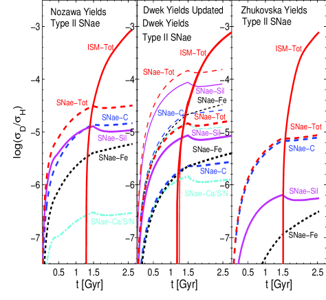
Figure 10: Temporal evolution of the contribution to the dust budget in the Solar Neighborhood during the first 1.5 Gyr-2.5 Gyr by type II SNæ according to three different prescriptions for the dust condensation efficiencies. All the contributions are already corrected for the effect of dust destruction. We show: the contribution by accretion of dust grains in the ISM (ISM-tot, continuous line); the total contribution by SNæ dust yields (SNæ-tot, dashed line); the contributions by the different kind of SNa dust grains, that is Silicates (SNæ-Sil, continuous line), carbonaceous grains (SNæ-C, dashed line), iron dust grains (SNæ-Fe, dotted line) and Ca/S/N generic dust grains (SNæ-Ca/S/N, dot-dashed line). Left panel: the results based on the Nozawa et al. (2003, 2006, 2007) condensation efficiencies. Central panel: the same as in the left panel but for the Dwek (1998) condensation efficiencies and for the Pipino et al. (2011) efficiencies. Right panel: the same as in the left panel but for the Calura et al. (2008) condensation efficiencies.

Let us start our analysis of different yields of dust by evaluating the effect of varying the amount of star-dust injected from type II SNæ. In the reference model identified by the parameter string $\mathcal{GDABBCBBB}$ we vary the recipe for dust yields (the sixth parameter of the string) choosing among the three possible solutions presented in Sect. 2, namely the one with high condensation efficiencies by Dwek (1998) and Calura et al. (2008), the set we built based upon the most CNT models for Type II SNæ by Nozawa et al. (2003, 2006, 2007), and the low SNæ efficiencies proposed by Zhukovska et al. (2008). We also included in the discussion the recently revised Dwek (1998) efficiencies, as proposed by Pipino et al. (2011) in order to reproduce the observational constraints: the coefficients for type II SNæ are lowered by a factor of 10. The results of the corresponding chemical models, with every parameter fixed except the use of different CCSNæ efficiencies, are presented in Fig. 10 where for simplicity we divided the contribution by SNæ grouping the elements in some typical grain families, silicates (like olivines, pyroxenes and quartz, depleting the gas of magnesium, silicon, iron and oxygen), carbonaceous grains, iron dust and other grains involving S/Ca/N (see Piovan et al. 2011b, for more details). The simulated region is the Solar Neighbourhood (SoNe) ring. Even if the SoNe region is not interested by an intense star formation activity, nevertheless in the early phases of the evolution, before that dust accretion in the ISM becomes significant, different efficiencies have a strong impact on the early evolution of the dust content. The CNT models present a contribution that is in the middle between low efficiencies by Zhukovska et al. (2008) and the high efficiencies by Dwek (1998). It is interesting to observe that the corrected contribution by Pipino et al. (2011), scaled in such a way to agree with the observations, also shown in the middle panel of Fig. 10 (thin lines), tends to produce similar total amount of dust as the CNT models. The relative contribution to the total mass budget of the elements embedded into dust grains is however quite different. It is interesting to underline the following point: Zhukovska et al. (2008) type II SNæ condensation efficiencies are chosen relying upon clues coming from pre-solar dust grains that seem to suggest a not negligible contribution of carbon based dust grains coming from SNæ. The level of carbonaceous grains formed adopting the Zhukovska et al. (2008) coefficient for carbon is similar to the one predicted by the revised ad-hoc efficiencies by Pipino et al. (2011) and the CNT models by Nozawa et al. (2003). This agreement seems satisfactory and it suggests some confidence in the carbon coefficient by Nozawa et al. (2003). However, it must be underlined that the recent 20M_⊙ and 170M_⊙ models by Cherchneff & Dwek (2010) with kinetic approach and following molecules evolution, do not form carbon based grains. The formation of carbon is hampered unless C-rich and He⁺ deprived regions are introduced, thus implying a strong dependence from the mixing induced by the explosion. Not even SiC is formed, however it is present in pre-solar dust grains (Hoppe et al. 2000). More detailed models are then probably required as well as more precise abundances of pre-solar dust grains, still highly uncertain.
For the refractory elements involved into the formation of silicates, the small number of detections of pre-solar grains does not allow a safe constraint. Zhukovska et al. (2008) assume a very low efficiency of condensation as working hypothesis, while in the other recipes that we included, a higher efficiency is chosen or comes out from CNT models. According to the results by Matsuura et al. (2011), this latter choice seems to be the most realistic one. They try to fit the emission spectrum of SN 1987A in the FIR/sub-mm observed with the PACS, using different combinations of typical dust grains. They find that a single dust species implies unrealistic dust masses. Therefore, a combinations of different dust grains is necessary. In this mixture, silicates are present as the most abundant species, thus suggesting that they condense in significant amounts. These recipes (Nozawa et al. 2003; Pipino et al. 2011) do not differ too much each other except from the original highly efficient Dwek (1998) recipe that produces a lot of dust. The kind of mixture of silicates anyway is strongly model dependent, and quite different partitions of grains are formed if we adopt the CNT hypothesis or the stochastic/kinetic models. We can therefore conclude that it is not so safe to follow the specific grain compounds that are injected into the ISM, due to the uncertainties on the specific mixture of dust produced. A bit more safe is to rely on a database like the one we calculated with the condensation efficiencies of the single elements, that in some way represents an average of the amount of an element involved into dust.

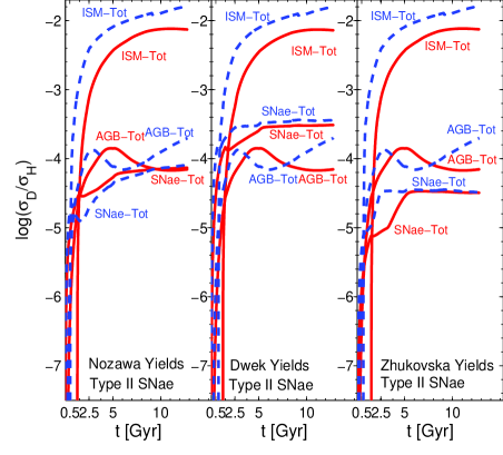
Figure 11: Temporal evolution of the contribution to the dust budget by type II SNæ according to three different prescriptions for the dust condensation efficiencies. The data refer to the Solar Neighbourhood (continuous lines) and the innermost region of the MW (dashed lines). All the contributions are already corrected for the effect of dust destruction. We show: the contribution by accretion of dust grain in the ISM (ISM-tot) and the total contributions by SNæ (SNæ-tot) and AGB stars (AGB-tot). Left panel: the results for the Nozawa et al. (2003, 2006, 2007) condensation efficiencies. Central panel: the same as in the left panel but for the Dwek (1998) and Calura et al. (2008) condensation efficiencies. Right panel: the same as in the left panel but for the Zhukovska et al. (2008) condensation efficiencies.

While the influence of different yields of dust by SNæ can be very important in the early stages of the evolution, once the accretion process in the ISM becomes the dominant dust factory and the SFR declines, there is in practice no influence on the relative dust budget compared to the gas amount at the current age, as clearly shown in Fig. 11. In this figure we present the evolution until the current time of three region of the MW, that are an inner ring around 2.3 Kpc (left panel), the Solar Neighbourhood at 8.5 Kpc (middle panel) and an outer ring at 15.1 Kpc (right panel). The three regions,from left to right, can be taken in some way as representative of three environments where a high/average/low star formation, respectively, occurred (Piovan et al. 2011b). The poor influence of the different recipes on the current total mass budget is true even for the innermost regions of the MW with higher SFR: once the accretion in MCs is the dominating process, the stardust injection becomes a secondary issue. The final dust content is controlled by dust accretion in the cold region of the ISM. In the same figure we also show for comparison the AGB reference contribution of the $\mathcal{GDABBCBBB}$ model based on the Ferrarotti & Gail (2006) and Zhukovska et al. (2008) estimate of the AGB efficiencies. Finally, it is interesting to note that different prescriptions for the dust yields by Type II SNæ cannot affect the amounts of the various elements embedded into dust in a low-star-forming environment in which the ISM is already enriched in atoms of metals and dust seeds. In these conditions the amount of free metals available in the ISM does not appreciably vary as a consequence of changes in the SNæ condensations, even in the case of SNæ yields dominating over those by AGB stars as in the model presented in the middle panel.

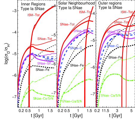
Figure 12: Temporal evolution of the contribution to the dust budget during the first 1.5 Gyr-2.5 Gyr by type Ia SNæ for two prescriptions of dust ejecta and three different regions of the MW: an inner ring at 2.3 Kpc, the SoNe, and an outer ring at 15.1 Kpc. The results for prescription $\mathcal{A}$ based on Dwek (1998); Calura et al. (2008) are represented with thin lines, whereas those for case $\mathcal{B}$ based on Zhukovska et al. (2008) are shown with thick lines. All the contributions are already corrected for the effect of dust destruction. We show: the contribution by accretion of dust grain in the ISM (ISM-tot, continuous lines); the total contribution by SNæ dust yields (SNæ-tot, type Ia + type II SNæ - continuous line); the contributions by the different kind of SNa dust grains, that is silicates (SNæ-Sil, continuous lines), carbonaceous grains (SNæ-C, dashed lines), iron dust grains (SNæ-Fe, dotted lines) and Ca/S/N based dust grains (SNæ-Ca/S/N, dot-dashed lines). Left panel: the results for the inner ring. Central panel: the same as in the left panel but for the SoNe. Right panel: the same as in the left panel but for the outer ring.

We turn now to examine the contribution to the dust content by Type Ia SNæ. Two different evaluations have been included into the model by Piovan et al. (2011b), namely one with high efficiency of dust formation by type Ia SNæ (see Dwek 1998, - our parameter n^o 5 in Tab. LABEL:Parameters, model $\mathcal{A}$) and one with very low efficiency, in closer agreement with the clues from observations (model $\mathcal{B}$). It must be underlined that in Pipino et al. (2011) the efficiency of condensation in type Ia SNæ by Calura et al. (2008) has been corrected from the high original value taken from Dwek (1998) to a much lower one, in order to satisfy what the observations actually tell us, that is no dust condensation is still observed in type Ia SNæ. In any case we want to explore the whole range of possibilities and for this reason we included two different solution. In Fig. 12 we present the evolution in the first Gyrs of the star-dust injected by the SNæ in three different regions of the MW Disk as before (left panel for the innermost regions, middle panel for the solar vicinity, right panel for the outermost one). The contribution by SNæ is in turn split according to the different types of grains that have been considered in Piovan et al. (2011a) and on which the single elements have been suitably grouped together. Finally, two models are displayed, one with high efficiency (thin lines) and one with low efficiency (thick lines). As expected, Type Ia SNæ do not affect the dust evolution during the first 0.5-1 Gyr, simply according to the current scenario for the origin of these objects since they still have to come in significant numbers. In brief, in the double-degenerate picture they start to contribute only after a certain amount of time has elapsed and their effect depends on the SFR history of the region. Furthermore, in the innermost regions, with high SFR and fast ISM enrichment, the dust accretion process starts to dominate early on the dust production and when type Ia SNæ come into play, it is already too late to have a significant role. However, in regions with low SFR such as the solar vicinity or, even more significantly, the outermost regions, it may happen that Type Ia SNæ significantly affect the dust enrichment, simply because the ISM accretion mechanism is delayed because of the poor enrichment in metals. This effect gets clearly stronger at lowering the SFR.

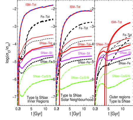
Figure 13: Temporal evolution up to 13 Gyr of the contribution to the dust budget by type Ia SNæ for two prescriptions of dust ejecta (models $\mathcal{A}$ and $\mathcal{B}$ of Fig. 12) and three different regions of the MW. The results for model $\mathcal{A}$ are represented by thin lines, whereas those of model $\mathcal{B}$ are indicated by thick lines. We show: the contribution by accretion of dust grain in the ISM (ISM-tot, continuous lines); the total evolution of the iron-dust (Fe-tot, dashed lines); the contributions by some of the SNa dust grains, that is silicates (SNæ-Sil, continuous lines), iron dust grains (SNæ-Fe, dotted lines) and Ca/S/N based dust grains (SNæ-Ca/S/N, dot-dashed lines). Left panel: the results for the inner ring. Central panel: the same but for the SoNe. Right panel: the same but for the outer ring.

Do different choices for the Type Ia SNæ condensation efficiencies influence the final depletion of the elements into dust at the current age? We show in Fig. 13 the evolution of the dust budget for our two different recipes for Type Ia SNæ: there is no difference in the ISM accretion process even for the low SFR environment. Even if the two recipes for the dust condensation in Type Ia SNæ produce very different amount of dust (see the thin and thick lines) this has no influence on the ISM process that mainly depends on the global amount of metals available in the ISM. We also checked what is the effect on the iron-dust budget: since Type Ia SNæ are the main iron polluters we would expect if not an effect on the global dust budget, at least some influence on the iron dust. Indeed, we find some differences, but only when we consider a low-star-forming environment. In that case the iron dust from SNæ can play a role in the final depletion. In the solar vicinity, on the contrary, at the present time no effect can be seen even if varying the condensation coefficients in Type Ia SNæ.

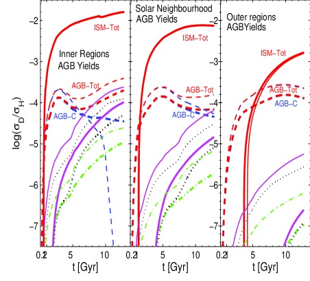
Figure 14: Temporal evolution of the contribution from AGB stars to the dust budget calculated until the present age. All the contributions have been properly corrected for the effect of dust destruction. Three regions of the MW Disk are considered as usual: the inner ring (left panel), the SoNe (middle panel), and the outer region (right panel). Thick lines represent our model $\mathcal{A}$ based upon Dwek (1998), whereas the thin lines represent model $\mathcal{B}$ based upon Ferrarotti & Gail (2006). We show: the total contribution by accretion of dust grain in the ISM (continuous lines) and the total contribution by AGB stars (dashed lines); the contributions by the various kinds of AGBs dust grains, in the specific: the iron-stardust (dotted lines); the silicates (continuous lines), the carbonaceous grains (dashed lines) and Ca/S/N based dust grains (dot-dashed lines). Left panel: The results for the inner ring. Central panel: the same as in the left panel but for the SoNe. Right panel: the same as in the left panel but for the outer ring.

Finally, we examine the role played by AGB stars that are long known to pollute the ISM with metals and dust of various kinds depending on the C/O ratio. In the very early stages of the evolution the contribution by AGB stars is negligible: since the most massive AGB star that we included in our models has 6 M_⊙, it takes some time before AGB stars start polluting the ISM. Depending on the condensation efficiency of the SNæ dust, if this latter is low it may happen that there could be a possibility for AGB stars to contribute significantly before the ISM accretion process starts dominating. In Fig. 14 we show the evolution of the AGB dust budget for the three regions of the MW disk for our two models $\mathcal{A}$ and $\mathcal{B}$ (see Table LABEL:Parameters). The difference between the models is less striking than for SNæ, with some exception like carbon evolution at high metallicities (left panel). Once more, dust production by ISM accretion overwhelms that by stars (the AGB stars in this case) and for low SFR (right panel - outer regions) we see a temporal window where AGB could produce some effect before the ISM accretion process becomes predominant. In any case we consider more reliable the use of the Ferrarotti & Gail (2006) models, that includes the effect of the metallicity on the development of the Carbon rich phase in the AGB, while the simple recipe by Dwek (1998); Calura et al. (2008); Pipino et al. (2011) do not take into account this point. The approach by which dust formation is simulated in the circumstellar envelope of AGB stars, in spite of its limitations, is more reliable than the hypotheses assumed for dust formation in SNæ (Cherchneff & Dwek 2010), and we can rely on Ferrarotti & Gail (2006) results. The inclusion of the metallicity effect allows to respect an important characteristic of the dust mixture: we have, as expected from AGB models, that low metallicity stars more easily enter the carbon rich phase and produce more carbon dust, while high metallicity stars, mainly avoiding or briefly entering the C-rich part of the evolution mainly contribute with silicates.
As we said, we fixed at 6 M_⊙ the transition between AGB stars and SNæ. In classical chemical models this limit typically varies from 5 to 8 M_⊙: this would have only a very small effect on the relative proportion of dust generated by SNæ and AGB stars, but it could affect the way by which AGB stars contribute to the early evolution (Valiante et al. 2009). Interestingly enough, recently a complete set of yields from S-AGB stars spanning the mass interval from 7.5 and 10.5 M_⊙ has been calculated (Siess 2010b, a). Even if the number of stars in this mass range nearly parallels the number of stars more massive than this limit (Siess 2010b), because of their short lifetime there are no firm evaluations of the role played by S-AGB stars in the chemical evolution of galaxies and even more important what could be their effect on the early evolution of the dust content in galaxies.

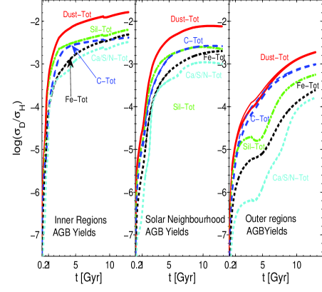
Figure 15: Temporal evolution of the contribution from AGB stars to the dust budget calculated until the present age. Three regions of the MW Disk are considered as usual: the inner ring (left panel), the SoNe (middle panel), and the outer region (right panel). Thick lines represent our model $\mathcal{A}$ based upon Dwek (1998), while thin lines represent model $\mathcal{B}$, based upon Ferrarotti & Gail (2006). We show: the total amount of dust grains in the ISM (continuous lines) and the total amount of the various grain families, where with total we mean AGB stardust plus SNæ stardust plus accreted dust in the ISM. In detail we show: the iron-stardust (dotted lines); the silicates (dot-dashed lines), the carbonaceous grains (dashed lines) and Ca/S/N based dust grains (dotted lines). Left panel: The results for the inner region of the MW Disk. Central panel: the same as in the left panel but for the SoNe. Right panel: the same as in the left panel but for the outer ring.

Does the different possible recipes for AGB star-dust lead to some differences in the evolution of the dust content in the ISM? In Fig. 15 we show (always for the three regions of the disk) the evolution of the total normalized abundance of the various dust grains families for the prescriptions for the AGB stars. Only in the outer regions with very low star formation rates and low metallicities we can notice a difference between one model of dust nucleation and injection by AGB stars and another. In the other regions, there is in practice no difference in the total budget at varying the AGB condensation efficiencies. This simply means that in the early stages, with the typical SF laws for the MW, AGB stars dust factory is dominated by SNæ (unless we assume a very low condensation efficiencies by SNæ), and later by the accretion process in the ISM. Obviously AGB stars play a fundamental role in refueling the ISM with metals and seeds, but the dust factory of the ISM accretion mechanism is the starring actor. Of course, if some peculiar dust grains (like SiC) are injected by AGBs and not formed by accretion in the ISM, in that case AGB stars play a crucial role in determining the evolution of that kind of dust.

5 Discussion and conclusions

In this paper we have described the database of condensation efficiencies for the main elements that form the dust emitted by the most important dust factories in nature, i.e. SNæ and AGB stars. The results are organized in tables containing the condensation efficiencies for the refractory elements C, O, Mg, Si, S, Ca (for this latter and partially for S, the average values between the condensation efficiencies of the other refractory elements has been adopted) and Fe in AGB stars and SNæ. The condensation efficiencies, multiplied by the gaseous ejecta provide an estimate of the amount of each element trapped into dust that is injected into the ISM. Our compilation stands upon the theoretical work by Ferrarotti & Gail (2006); Zhukovska et al. (2008) and Nozawa et al. (2003, 2006, 2007) and allows us to take into account: (1) the different metallicity of the AGB stars, thus simulating the growing number of C-rich stars forming carbonaceous grains at lowering the metallicity; (2) the different density of the environment in which the SNa explosion occurs which crucially determines the final amount of dust surviving to the shocks.
There is an important aspect of the results to note. The mixture of dust grains emitted by stars, in particular the one by SNæ, is still very model dependent: for instance the kinetic models by Cherchneff & Dwek (2010) not only predict different total amounts of dust as compared to the classical CNT models by Nozawa et al. (2003), but also different composition for the dust. To somehow cure this point of uncertainty we calculated (and tested) average condensation coefficients for each elements. To this aim, we made use of the best prescriptions for the production of dust by stars, and compared the results one would obtain by introducing them in the classical chemical model for the MW Disk and SoNe (Piovan et al. 2011b, c). As already mentioned, the largest uncertainty is due to SNæ: to highlight the point we compare the model results with the available data about the amounts of dust and its composition, taking into account the observational hints by pre-solar grains and IR emission from SNa remnants. In particular we look for the best solution to be adopted for SNæ. We find that the CNT approximation widely adopted for dust formation in SNæ, despite its limitations as a first order approximation of a complex situation neither at equilibrium nor at steady state, still gives good results. Indeed, (i) it produces amounts of carbonaceous grains that agree with the estimate required by the pre-solar dust grains; (ii) it produces significant amounts of silicates that seem to be necessary to reproduce very recent cold dust emission spectra in the SN 1987A; (iii) the amount of dust produced by SNæ is not negligible, as indicated by the most recent in observations at long wavelengths and, (iv) the CNT unmixed model agrees well with both the FIR/sub-mm estimates of newly formed dust in SNæ and the amount of dust required to explain high-z obscured objects with the SNæ playing a decisive role.
The whole picture we have just outlined could be considered as satisfactory. However, it is worth noticing: (i) the reduction in the amount of dust predicted by the more physically correct kinetic models, goes in the opposite direction with respect to what indicated by observations of cold dust; (ii) the poor data available on pre-solar silicates does not support an efficient condensation of silicates as indicated by estimates of cold dust in SNæ.
This simply means that our understanding of dust formation in SNæ is still very uncertain, both theoretically and observationally. More data on cold dust for a wider sample of SNæ is needed. A new generation of models of dust formation in SNæ is therefore required to highlight the many points of uncertainty and contradiction. They go from the obvious uncertainty in the correct approach to use, the complicated description of the dust formation and the the limited number of accurate models in literature to poor statistics, lack of high quality observations of the cold dust in the FIR/sub-mm for many SNæ, and uncertainties on estimating the amount of fresh dust).

Acknowledgements. L. Piovan acknowledges A. Weiss and the Max Planck Institut Fur AstroPhysik (Garching - Germany) for the very warm and friendly hospitality and providing unlimited computational support during the visits as EARA fellow when a significant part of this study has been carried out. The authors are also deeply grateful to S. Zhukovska and H. P. Gail for many explanations and clarifications about their yields of dust from AGB stars, T. Nozawa and H. Umeda for many fruitful discussions about SNa dust yields. This work has been financed by the University of Padua with the dedicated fellowship ”Numerical Simulations of galaxies (dynamical, chemical and spectrophotometric models), strategies of parallelization in dynamical lagrangian approach, communication cell-to-cell into hierarchical tree codes, algorithms and optimization techniques” as part of the AACSE Strategic Research Project.

Appendix A

The models of dust formation in the ejecta of Pop III CCSNæ (core collapse) and PISNæ (pair-instability) by Nozawa et al. (2003) are obtained taking into account two extreme cases, i.e. no mixing and full mixing in the He core. In the un-mixed case the typical onion-like structure is considered. In the uniformly mixed model all the elements are mixed in the He core. In both cases many types of dust grain are considered: Fe, FeS, Si, V, T, Cr, Co, Ni, Cu, C, SiC, TiC, Al₂O₃, MgSiO₃, Mg₂SiO₄, SiO₂, MgO, Fe₃O₄, FeO. In the final yields of dust, only some of these species are present. In the un-mixed case we have Fe, FeS, Si, C, Al₂O₃, MgSiO₃, Mg₂SiO₄, SiO₂ and MgO, whereas for the mixed one we have SiO₂, Al₂O₃, MgSiO₃, Mg₂SiO₄ and Fe₃O₄. For the abundances of the single elements in the yields of dust of the $i$-th progenitor we used the following equations. For the unmixed case:

$$M_{i} \left(C\right)=M_{i}\left(C\right)$$ (15)

$$M_{i} \left(O\right)=A\left(O\right)\left[\frac{4M_{i}\left(MgSiO_{4}\right)}{A\left(MgSiO_{4}\right)}+\frac{3M_{i}\left(MgSiO_{3}\right)}{A\left(MgSiO_{3}\right)}+\right.$$

$$+\left.\frac{3M_{i}\left(Al_{2}O_{3}\right)}{A\left(Al_{2}O_{3}\right)}+\frac{M_{i}\left(2SiO_{2}\right)}{A\left(SiO_{2}\right)}+\frac{M_{i}\left(MgO\right)}{A\left(MgO\right)}\right]$$ (16)

$$M_{i} \left(Mg\right)=A\left(Mg\right)\left[\frac{M_{i}\left(MgSiO_{3}\right)}{A\left(MgSiO_{3}\right)}+\frac{M_{i}\left(MgSiO_{4}\right)}{A\left(MgSiO_{4}\right)}+\right.$$

$$+\left.\frac{M_{i}\left(MgO\right)}{A\left(MgO\right)}\right]$$ (17)

$$M_{i} \left(Si\right)=A\left(Si\right)\left[\frac{M_{i}\left(MgSiO_{3}\right)}{A\left(MgSiO_{3}\right)}+\frac{M_{i}\left(MgSiO_{4}\right)}{A\left(MgSiO_{4}\right)}+\right.$$

$$+\left.\frac{M_{i}\left(Si\right)}{A\left(Si\right)}+\frac{M_{i}\left(SiO_{2}\right)}{A\left(SiO_{2}\right)}\right]$$ (18)

$$M_{i} \left(S\right)=A\left(S\right)\frac{M_{i}\left(FeS\right)}{A\left(FeS\right)}$$ (19)

$$M_{i} \left(Fe\right)=A\left(Fe\right)\left[\frac{M_{i}\left(Fe\right)}{A\left(Fe\right)}+\frac{M_{i}\left(FeS\right)}{A\left(FeS\right)}\right]$$ (20)

where $A\left(...\right)$ are the mass numbers of the considered elements or molecules and $M_{i}\left(...\right)$ are the dust yields of a given element or molecule for the $i$-th progenitor. For the mixed case the equations in use are:

$$M_{i} \left(O\right)=A\left(O\right)\left[\frac{4M_{i}\left(MgSiO_{4}\right)}{A\left(MgSiO_{4}\right)}+\frac{3M_{i}\left(MgSiO_{3}\right)}{A\left(MgSiO_{3}\right)}+\right.$$

$$+\left.\frac{3M_{i}\left(Al_{2}O_{3}\right)}{A\left(Al_{2}O_{3}\right)}+\frac{M_{i}\left(2SiO_{2}\right)}{A\left(SiO_{2}\right)}+\frac{3M_{i}\left(Al_{2}O_{3}\right)}{A\left(Al_{2}O_{3}\right)}\right]$$ (21)

$$M_{i} \left(Mg\right)=A\left(Mg\right)\left[\frac{M_{i}\left(MgSiO_{3}\right)}{A\left(MgSiO_{3}\right)}+\frac{M_{i}\left(MgSiO_{4}\right)}{A\left(MgSiO_{4}\right)}\right]$$ (22)

$$M_{i} \left(Si\right)=A\left(Si\right)\left[\frac{M_{i}\left(MgSiO_{3}\right)}{A\left(MgSiO_{3}\right)}+\frac{M_{i}\left(MgSiO_{4}\right)}{A\left(MgSiO_{4}\right)}+\right.$$

$$+\left.\frac{M_{i}\left(SiO_{2}\right)}{A\left(SiO_{2}\right)}\right]$$ (23)

$$M_{i} \left(Fe\right)=A\left(Fe\right)\left[\frac{3M_{i}\left(Fe_{3}O_{4}\right)}{A\left(Fe_{3}O_{4}\right)}\right]$$ (24)

In this latter case, Aluminium $M_{i}\left(Al\right)$ is not taken into account, because our chemical model does not include the evolution of this element.

Appendix B

According to Zhukovska et al. (2008), dust formation in AGB stars has been interpolated and extrapolated from the data and models by Ferrarotti & Gail (2006) to eight metallicities, going from $Z=0.001$ to $Z=0.04$ and to a set of twenty-seven masses from $1$M_⊙ to $7$M_⊙. Three types of mixtures are considered depending on the C/O ratio, i.e. for M-stars, S-stars and C-stars. For M-stars they consider the formation of the following dust molecules: (1) magnesium iron silicates, like the olivines forsterite (Mg₂SiO₄, with Mg as the end-member) and fayalite (Fe₂SiO₄, with Fe as the end-member), the pyroxenes enstatite (MgSiO₃, with Mg as the end-member), and ferrosilite (FeSiO₃, with Fe as the end-member); (2) quartz SiO₂ and (3) iron dust grains Fe. For S-stars they only consider (1) quartz SiO₂ and (2) iron dust grains Fe, while for carbon rich C-stars they include (1) carbonaceous grains made by C and H, again (2) quartz SiO₂ and (3) iron dust grains Fe.

For the abundances of the single elements in the dust yields of the $i$-th progenitor we used the following equations:

For $M$-stars

$$M_{i} \left(O\right)=A\left(O\right)\left[\frac{4M_{i}\left(MgSiO_{4}\right)}{A\left(MgSiO_{4}\right)}+\frac{3M_{i}\left(MgSiO_{3}\right)}{A\left(MgSiO_{3}\right)}+\right.$$

$$+\left.\frac{4M_{i}\left(FeSiO_{4}\right)}{A\left(FeSiO_{4}\right)}+\frac{3M_{i}\left(FeSiO_{3}\right)}{A\left(FeSiO_{3}\right)}+\frac{M_{i}\left(2SiO_{2}\right)}{A\left(SiO_{2}\right)}\right]$$ (25)

$$M_{i} \left(Mg\right)=A\left(Mg\right)\left[\frac{M_{i}\left(MgSiO_{3}\right)}{A\left(MgSiO_{3}\right)}+\frac{M_{i}\left(MgSiO_{4}\right)}{A\left(MgSiO_{4}\right)}\right]$$ (26)

$$M_{i} \left(Si\right)=A\left(Si\right)\left[\frac{M_{i}\left(MgSiO_{3}\right)}{A\left(MgSiO_{3}\right)}+\frac{M_{i}\left(MgSiO_{4}\right)}{A\left(MgSiO_{4}\right)}+\right.$$

$$+\left.\frac{M_{i}\left(SiO_{2}\right)}{A\left(SiO_{2}\right)}\right]$$ (27)

$$M_{i} \left(Fe\right)=A\left(Fe\right)\left[\frac{M_{i}\left(FeSiO_{4}\right)}{A\left(FeSiO_{4}\right)}+\frac{M_{i}\left(FeSiO_{3}\right)}{A\left(FeSiO_{3}\right)}+\right.$$

$$+\left.\frac{M_{i}\left(Fe\right)}{A\left(Fe\right)}\right]$$ (28)

where $A\left(...\right)$ are the mass numbers of the considered elements or molecules and $M_{i}\left(...\right)$ are the dust yields of a given element or molecule for the $i$-th progenitor.

For $S$-stars

$$M_{i} \left(O\right)=A\left(O\right)\left[\frac{2M_{i}\left(SiO_{2}\right)}{A\left(SiO_{2}\right)}\right]$$ (29)

$$M_{i} \left(Si\right)=A\left(Si\right)\left[\frac{M_{i}\left(SiO_{2}\right)}{A\left(SiO_{2}\right)}\right]$$ (30)

$$M_{i} \left(Fe\right)=A\left(Fe\right)\left[\frac{M_{i}\left(Fe\right)}{A\left(Fe\right)}\right]$$ (31)

Finally, for C-stars

$$M_{i} \left(Si\right)=A\left(Si\right)\left[\frac{M_{i}\left(SiC\right)}{A\left(SiC\right)}\right]$$ (32)

$$M_{i} \left(C\right)=A\left(C\right)\left[\frac{M_{i}\left(C\right)}{A\left(C\right)}+\frac{M_{i}\left(SiC\right)}{A\left(SiC\right)}\right]$$ (33)

$$M_{i} \left(Fe\right)=A\left(Fe\right)\left[\frac{M_{i}\left(Fe\right)}{A\left(Fe\right)}\right]$$ (34)

with the usual meaning of the symbols.

Table 4: Dust condensation efficiencies for AGB stars of metallicity Z=0.001.

M⊙	$\delta_{C}$	$\delta_{O}$	$\delta_{Mg}$	$\delta_{Si}$	$\delta_{Fe}$	$\delta_{Ca}$	$\delta_{S}$	$\delta_{Al}$
1.00	0.00000000	0.00000000	0.00000000	0.00000000	0.00000000	0.00000000	0.00000000	0.00000000
1.10	0.00481670	0.00000000	0.00000000	0.00000000	0.00000000	0.00000000	0.00000000	0.00000000
1.20	0.14639919	0.00000000	0.00000000	0.00000000	0.00000000	0.00000000	0.00000000	0.00000000
1.25	0.18576120	0.00000000	0.00000000	0.00000000	0.00000000	0.00000000	0.00000000	0.00000000
1.30	0.23425915	0.00000000	0.00000000	0.00000000	0.00000000	0.00000000	0.00000000	0.00000000
1.40	0.29019752	0.00000000	0.00000000	0.00000000	0.00000000	0.00000000	0.00000000	0.00000000
1.50	0.39619540	0.00000000	0.00000000	0.00000000	0.00000000	0.00000000	0.00000000	0.00000000
1.60	0.45922137	0.00000000	0.00000000	0.00000000	0.00000000	0.00000000	0.00000000	0.00000000
1.70	0.52030200	0.00000000	0.00000000	0.00000000	0.00000000	0.00000000	0.00000000	0.00000000
1.80	0.53833388	0.00000000	0.00000000	0.00003080	0.00000000	0.00001026	0.00001026	0.00001026
1.90	0.50111438	0.00000000	0.00000000	0.00003117	0.00000000	0.00001039	0.00001039	0.00001039
2.00	0.47470917	0.00000000	0.00000000	0.00003262	0.00000000	0.00001087	0.00001087	0.00001087
2.10	0.46005052	0.00000000	0.00000000	0.00003321	0.00000000	0.00001107	0.00001107	0.00001107
2.20	0.45734066	0.00000000	0.00000000	0.00003437	0.00000000	0.00001145	0.00001145	0.00001145
2.30	0.46136134	0.00000000	0.00000000	0.00003487	0.00000000	0.00001162	0.00001162	0.00001162
2.40	0.46360417	0.00000000	0.00000000	0.00003586	0.00000000	0.00001195	0.00001195	0.00001195
2.50	0.45318091	0.00000000	0.00000000	0.00003663	0.00000000	0.00001221	0.00001221	0.00001221
3.00	0.47763680	0.00000000	0.00000000	0.00004363	0.00000000	0.00001454	0.00001454	0.00001454
3.50	0.53036135	0.00000000	0.00000000	0.00004637	0.00000000	0.00001545	0.00001545	0.00001545
4.00	1.00000000	0.00000000	0.00000000	0.00004927	0.00000000	0.00001642	0.00001642	0.00001642
4.50	0.15586482	0.00000014	0.00000006	0.00002279	0.00001202	0.00001162	0.00001162	0.00001162
5.00	0.14262594	0.00000033	0.00000008	0.00002682	0.00001382	0.00001357	0.00001357	0.00001357
5.50	0.12204322	0.00000049	0.00000008	0.00002615	0.00001530	0.00001384	0.00001384	0.00001384
6.00	0.10409485	0.00000073	0.00000007	0.00002593	0.00001666	0.00001422	0.00001422	0.00001422
6.50	0.09531371	0.00000081	0.00000006	0.00002658	0.00001798	0.00001487	0.00001487	0.00001487
7.00	0.08813571	0.00000083	0.00000006	0.00002702	0.00001928	0.00001545	0.00001545	0.00001545

Table 5: Dust condensation efficiencies for AGB stars of metallicity Z=0.002.

M⊙	$\delta_{C}$	$\delta_{O}$	$\delta_{Mg}$	$\delta_{Si}$	$\delta_{Fe}$	$\delta_{Ca}$	$\delta_{S}$	$\delta_{Al}$
1.00	0.00000000	0.00000000	0.00000000	0.00000000	0.00000000	0.00000000	0.00000000	0.00000000
1.10	0.00265956	0.00000000	0.00000000	0.00000000	0.00000000	0.00000000	0.00000000	0.00000000
1.20	0.15026726	0.00000000	0.00000000	0.00003450	0.00000000	0.00001150	0.00001150	0.00001150
1.25	0.15487339	0.00000000	0.00000000	0.00004420	0.00000000	0.00001473	0.00001473	0.00001473
1.30	0.21380446	0.00000000	0.00000000	0.00006667	0.00000000	0.00002222	0.00002222	0.00002222
1.40	0.29515964	0.00000000	0.00000000	0.00010309	0.00000000	0.00003436	0.00003436	0.00003436
1.50	0.36691218	0.00000102	0.00000000	0.00015487	0.00000000	0.00005162	0.00005162	0.00005162
1.60	0.39952639	0.00000000	0.00000000	0.00012928	0.00000000	0.00004309	0.00004309	0.00004309
1.70	0.41162551	0.00000000	0.00000000	0.00012490	0.00000000	0.00004163	0.00004163	0.00004163
1.80	0.42151132	0.00000000	0.00000000	0.00013551	0.00000000	0.00004517	0.00004517	0.00004517
1.90	0.41303055	0.00000000	0.00000000	0.00014318	0.00000000	0.00004772	0.00004772	0.00004772
2.00	0.40014155	0.00000000	0.00000000	0.00015340	0.00000000	0.00005113	0.00005113	0.00005113
2.10	0.37498383	0.00000000	0.00000000	0.00015437	0.00000000	0.00005145	0.00005145	0.00005145
2.20	0.38755967	0.00000000	0.00000000	0.00015997	0.00000000	0.00005332	0.00005332	0.00005332
2.30	0.37049519	0.00000000	0.00000000	0.00016498	0.00000000	0.00005499	0.00005499	0.00005499
2.40	0.37186737	0.00000000	0.00000000	0.00016891	0.00000000	0.00005630	0.00005630	0.00005630
2.50	0.36282426	0.00000000	0.00000000	0.00017613	0.00000000	0.00005871	0.00005871	0.00005871
3.00	0.34320933	0.00000000	0.00000000	0.00021219	0.00000000	0.00007073	0.00007073	0.00007073
3.50	0.46943942	0.00000000	0.00000000	0.00024423	0.00000000	0.00008141	0.00008141	0.00008141
4.00	1.00000000	0.00000000	0.00000000	0.00027761	0.00000000	0.00009253	0.00009253	0.00009253
4.50	0.12055474	0.00000142	0.00000059	0.00011654	0.00006326	0.00006013	0.00006013	0.00006013
5.00	0.10926296	0.00000177	0.00000053	0.00012074	0.00007193	0.00006440	0.00006440	0.00006440
5.50	0.09486079	0.00000242	0.00000052	0.00012001	0.00007762	0.00006605	0.00006605	0.00006605
6.00	0.08336151	0.00000323	0.00000044	0.00011962	0.00008168	0.00006725	0.00006725	0.00006725
6.50	0.07595158	0.00000366	0.00000043	0.00012366	0.00008886	0.00007098	0.00007098	0.00007098
7.00	0.07009158	0.00000393	0.00000043	0.00012864	0.00009646	0.00007518	0.00007518	0.00007518

Table 6: Dust condensation efficiencies for AGB stars of metallicity Z=0.004.

M⊙	$\delta_{C}$	$\delta_{O}$	$\delta_{Mg}$	$\delta_{Si}$	$\delta_{Fe}$	$\delta_{Ca}$	$\delta_{S}$	$\delta_{Al}$
1.00	0.00000000	0.00000000	0.00000000	0.00000000	0.00000000	0.00000000	0.00000000	0.00000000
1.10	0.00083222	0.00000000	0.00000000	0.00000000	0.00000000	0.00000000	0.00000000	0.00000000
1.20	0.09697428	0.00000000	0.00000000	0.00034345	0.00000000	0.00011448	0.00011448	0.00011448
1.25	0.21074678	0.00000000	0.00000000	0.00092058	0.00000000	0.00030686	0.00030686	0.00030686
1.30	0.25507001	0.00000000	0.00000000	0.00108098	0.00000000	0.00036032	0.00036032	0.00036032
1.40	0.33996781	0.00000000	0.00000000	0.00123257	0.00000000	0.00041085	0.00041085	0.00041085
1.50	0.40811000	0.00000000	0.00000000	0.00144564	0.00000000	0.00048188	0.00048188	0.00048188
1.60	0.44345154	0.00000000	0.00000000	0.00153059	0.00000000	0.00051019	0.00051019	0.00051019
1.70	0.45103152	0.00000000	0.00000000	0.00146990	0.00000000	0.00048996	0.00048996	0.00048996
1.80	0.48278305	0.00000000	0.00000000	0.00155159	0.00000000	0.00051719	0.00051719	0.00051719
1.90	0.52098757	0.00000000	0.00000000	0.00159094	0.00000000	0.00053031	0.00053031	0.00053031
2.00	0.49801535	0.00000000	0.00000000	0.00162689	0.00000000	0.00054229	0.00054229	0.00054229
2.10	0.50604017	0.00000000	0.00000000	0.00155156	0.00000000	0.00051718	0.00051718	0.00051718
2.20	0.51122053	0.00000000	0.00000000	0.00171615	0.00000000	0.00057205	0.00057205	0.00057205
2.30	0.52421529	0.00000000	0.00000000	0.00164786	0.00000000	0.00054928	0.00054928	0.00054928
2.40	0.51358635	0.00000000	0.00000000	0.00171132	0.00000000	0.00057044	0.00057044	0.00057044
2.50	0.52089403	0.00000258	0.00000000	0.00177490	0.00000000	0.00059163	0.00059163	0.00059163
3.00	0.58487881	0.00000000	0.00000000	0.00204975	0.00000385	0.00068453	0.00068453	0.00068453
3.50	0.40179017	0.00000000	0.00000000	0.00336510	0.00000554	0.00112355	0.00112355	0.00112355
4.00	1.00000000	0.00000000	0.00000000	0.00410518	0.00000553	0.00137024	0.00137024	0.00137024
4.50	0.07722777	0.00002405	0.00001569	0.00123602	0.00088501	0.00071224	0.00071224	0.00071224
5.00	0.06873504	0.00002940	0.00001430	0.00129496	0.00099224	0.00076717	0.00076717	0.00076717
5.50	0.06051039	0.00003360	0.00001203	0.00132337	0.00099961	0.00077834	0.00077834	0.00077834
6.00	0.05301306	0.00003907	0.00000986	0.00130422	0.00102121	0.00077843	0.00077843	0.00077843
6.50	0.04938816	0.00004243	0.00000911	0.00136929	0.00107905	0.00081915	0.00081915	0.00081915
7.00	0.04591880	0.00004523	0.00000880	0.00138212	0.00113674	0.00084255	0.00084255	0.00084255

Table 7: Dust condensation efficiencies for AGB stars of metallicity Z=0.008.

M⊙	$\delta_{C}$	$\delta_{O}$	$\delta_{Mg}$	$\delta_{Si}$	$\delta_{Fe}$	$\delta_{Ca}$	$\delta_{S}$	$\delta_{Al}$
1.00	0.00000000	0.00000000	0.00000000	0.00000000	0.00000000	0.00000000	0.00000000	0.00000000
1.10	0.00027758	0.00009887	0.00036252	0.00132490	0.00261710	0.00143484	0.00143484	0.00143484
1.20	0.07760180	0.00059906	0.00212571	0.01598957	0.02168562	0.01326697	0.01326697	0.01326697
1.25	0.07606858	0.00030102	0.00105843	0.03153497	0.01847338	0.01702226	0.01702226	0.01702226
1.30	0.14477275	0.00028493	0.00100876	0.03348390	0.00776547	0.01408604	0.01408604	0.01408604
1.40	0.15255537	0.00025173	0.00093851	0.03289920	0.00726190	0.01369987	0.01369987	0.01369987
1.50	0.15482117	0.00000000	0.00000000	0.03063335	0.00022130	0.01028488	0.01028488	0.01028488
1.60	0.22931682	0.00000000	0.00000000	0.03446039	0.00013123	0.01153054	0.01153054	0.01153054
1.70	0.29105982	0.00000000	0.00000000	0.03601382	0.00006852	0.01202745	0.01202745	0.01202745
1.80	0.32492563	0.00000000	0.00000000	0.03546248	0.00005612	0.01183953	0.01183953	0.01183953
1.90	0.35826111	0.00000000	0.00000000	0.03614184	0.00003385	0.01205856	0.01205856	0.01205856
2.00	0.39031755	0.00000000	0.00000000	0.03749559	0.00003115	0.01250891	0.01250891	0.01250891
2.10	0.42299855	0.00000000	0.00000000	0.03821450	0.00002576	0.01274675	0.01274675	0.01274675
2.20	0.43290204	0.00000000	0.00000000	0.03648384	0.00002441	0.01216942	0.01216942	0.01216942
2.30	0.45596038	0.00000000	0.00000000	0.03759902	0.00002318	0.01254073	0.01254073	0.01254073
2.40	0.46422409	0.00000000	0.00000000	0.04062868	0.00002216	0.01355028	0.01355028	0.01355028
2.50	0.48453652	0.00000000	0.00000000	0.03974079	0.00002097	0.01325392	0.01325392	0.01325392
3.00	0.57992976	0.00000000	0.00000000	0.04517592	0.00001616	0.01506402	0.01506402	0.01506402
3.50	0.29496188	0.00000000	0.00000000	0.06281384	0.00003823	0.02095069	0.02095069	0.02095069
4.00	0.86459902	0.00000000	0.00000000	0.06980109	0.00003735	0.02327948	0.02327948	0.02327948
4.50	0.03021447	0.00779002	0.01101550	0.10334552	0.14612063	0.08682722	0.08682722	0.08682722
5.00	0.03000158	0.00816375	0.00846570	0.10708606	0.14715856	0.08757011	0.08757011	0.08757011
5.50	0.02708609	0.00923751	0.00761757	0.10935401	0.14469343	0.08722167	0.08722167	0.08722167
6.00	0.02422391	0.01037559	0.00670013	0.11334449	0.14625306	0.08876589	0.08876589	0.08876589
6.50	0.02282019	0.01068092	0.00606410	0.11320376	0.14183756	0.08703514	0.08703514	0.08703514
7.00	0.02128779	0.01095849	0.00561900	0.11206287	0.13593213	0.08453800	0.08453800	0.08453800

Table 8: Dust condensation efficiencies for AGB stars of metallicity Z=0.015.

M⊙	$\delta_{C}$	$\delta_{O}$	$\delta_{Mg}$	$\delta_{Si}$	$\delta_{Fe}$	$\delta_{Ca}$	$\delta_{S}$	$\delta_{Al}$
1.00	0.00000000	0.01622151	0.10337936	0.19067569	0.26824351	0.18743286	0.18743286	0.18743286
1.10	0.00000000	0.01989686	0.11994899	0.23451746	0.31372527	0.22273057	0.22273057	0.22273057
1.20	0.00000000	0.01897280	0.10806979	0.22449623	0.29882128	0.21046243	0.21046243	0.21046243
1.25	0.00000000	0.01940105	0.10893929	0.23035203	0.29258844	0.21062658	0.21062658	0.21062658
1.30	0.00000000	0.02117347	0.11832043	0.25223618	0.31781088	0.22945583	0.22945583	0.22945583
1.40	0.00000000	0.01880107	0.10771517	0.22584695	0.30122424	0.21159545	0.21159545	0.21159545
1.50	0.01612098	0.01844121	0.10805736	0.24602971	0.31441874	0.22283527	0.22283527	0.22283527
1.60	0.00187487	0.01829934	0.10631659	0.22389462	0.33054988	0.22025369	0.22025369	0.22025369
1.70	0.03372210	0.01095275	0.06322135	0.18120554	0.55583957	0.26675549	0.26675549	0.26675549
1.80	0.05378203	0.00771053	0.00727006	0.24215832	0.11816384	0.12253074	0.12253074	0.12253074
1.90	0.10033417	0.00123331	0.00688251	0.17667234	0.04297937	0.07551141	0.07551141	0.07551141
2.00	0.17177962	0.00117904	0.00650155	0.33888422	0.15096066	0.16544881	0.16544881	0.16544881
2.10	0.22003572	0.00084726	0.00461739	0.31107965	0.02916475	0.11495393	0.11495393	0.11495393
2.20	0.26818177	0.00062284	0.00344337	0.29958994	0.02299745	0.10867692	0.10867692	0.10867692
2.30	0.31008388	0.00141144	0.00000089	0.32679560	0.00348235	0.11009295	0.11009295	0.11009295
2.40	0.34559179	0.00000010	0.00000059	0.28613619	0.00427951	0.09680543	0.09680543	0.09680543
2.50	0.36478837	0.00000000	0.00000000	0.29653113	0.00712501	0.10121871	0.10121871	0.10121871
3.00	0.53051299	0.00000000	0.00000000	0.29465242	0.00022888	0.09829376	0.09829376	0.09829376
3.50	0.34012190	0.00000000	0.00000000	0.33390767	0.00067675	0.11152814	0.11152814	0.11152814
4.00	0.28373240	0.00000000	0.00000000	0.40260222	0.00445742	0.13568654	0.13568654	0.13568654
4.50	0.00883125	0.02274328	0.06481755	0.27767137	0.26289180	0.20179357	0.20179357	0.20179357
5.00	0.00763527	0.02265625	0.05189337	0.27938663	0.24193878	0.19107293	0.19107293	0.19107293
5.50	0.00685113	0.02352466	0.04558380	0.27452172	0.23402431	0.18470995	0.18470995	0.18470995
6.00	0.00577691	0.02453750	0.03980196	0.26985066	0.22267650	0.17744304	0.17744304	0.17744304
6.50	0.00555197	0.02492647	0.03636159	0.26652971	0.21356319	0.17215149	0.17215149	0.17215149
7.00	0.00502738	0.02528332	0.03375876	0.26303478	0.20576146	0.16751834	0.16751834	0.16751834

Table 9: Dust condensation efficiencies for AGB stars of metallicity Z=0.02.

M⊙	$\delta_{C}$	$\delta_{O}$	$\delta_{Mg}$	$\delta_{Si}$	$\delta_{Fe}$	$\delta_{Ca}$	$\delta_{S}$	$\delta_{Al}$
1.00	0.00000000	0.03588087	0.28188633	0.42317978	0.48590908	0.39699173	0.39699173	0.39699173
1.10	0.00000000	0.03744050	0.27525320	0.44111016	0.51543185	0.41059841	0.41059841	0.41059841
1.20	0.00000000	0.04159802	0.28644563	0.48998219	0.54661994	0.44101592	0.44101592	0.44101592
1.25	0.00000000	0.04468728	0.30066679	0.52663114	0.58942348	0.47224047	0.47224047	0.47224047
1.30	0.00000000	0.03918550	0.26010042	0.46278830	0.51112469	0.41133780	0.41133780	0.41133780
1.40	0.00000000	0.03815650	0.25531810	0.45374694	0.49276080	0.40060861	0.40060861	0.40060861
1.50	0.00000000	0.03755734	0.25306780	0.44863829	0.50755628	0.40308746	0.40308746	0.40308746
1.60	0.00000000	0.03523968	0.23093010	0.42641801	0.45943436	0.37226082	0.37226082	0.37226082
1.70	0.01731944	0.03372272	0.21993045	0.42843372	0.46029551	0.36955323	0.36955323	0.36955323
1.80	0.00747658	0.03313635	0.21398305	0.42163598	0.49490421	0.37684108	0.37684108	0.37684108
1.90	0.03012721	0.03244870	0.20786083	0.43504426	0.55978612	0.40089707	0.40089707	0.40089707
2.00	0.03783436	0.02008472	0.12747051	0.27485541	0.50827910	0.30353501	0.30353501	0.30353501
2.10	0.07491230	0.00273484	0.01705400	0.26454065	0.41019760	0.23059742	0.23059742	0.23059742
2.20	0.10537837	0.00442499	0.01136481	0.33324845	0.16352652	0.16937993	0.16937993	0.16937993
2.30	0.16635710	0.00219678	0.00294874	0.41019668	0.09997012	0.17103852	0.17103852	0.17103852
2.40	0.28411965	0.00072087	0.00000080	0.55655533	0.13558008	0.23071207	0.23071207	0.23071207
2.50	0.30505662	0.00072684	0.00000000	0.55319755	0.02987900	0.19435885	0.19435885	0.19435885
3.00	0.47605672	0.00000000	0.00000000	0.49814355	0.00150995	0.16655116	0.16655116	0.16655116
3.50	0.38344394	0.00000000	0.00000000	0.54722350	0.00311482	0.18344611	0.18344611	0.18344611
4.00	0.30805414	0.00000005	0.00000028	0.60713409	0.00867781	0.20527073	0.20527073	0.20527073
4.50	0.00340680	0.03293037	0.13415468	0.39329761	0.32212277	0.28319169	0.28319169	0.28319169
5.00	0.00211536	0.03241885	0.11598430	0.38785476	0.29799660	0.26727855	0.26727855	0.26727855
5.50	0.00284376	0.03312643	0.10431749	0.37975338	0.27933865	0.25446984	0.25446984	0.25446984
6.00	0.00253550	0.03402182	0.09563033	0.37537577	0.26596970	0.24565860	0.24565860	0.24565860
6.50	0.00224815	0.03448482	0.09007775	0.36997262	0.25614723	0.23873253	0.23873253	0.23873253
7.00	0.00202929	0.03486064	0.08524557	0.36396209	0.24701413	0.23207393	0.23207393	0.23207393

Table 10: Dust condensation efficiencies for AGB stars of metallicity Z=0.03.

M⊙	$\delta_{C}$	$\delta_{O}$	$\delta_{Mg}$	$\delta_{Si}$	$\delta_{Fe}$	$\delta_{Ca}$	$\delta_{S}$	$\delta_{Al}$
1.00	0.00000000	0.07082836	0.75108259	0.83103533	0.98354473	0.85522088	0.85522088	0.85522088
1.10	0.00000000	0.07613366	0.75363042	0.89351633	1.00000000	0.88238225	0.88238225	0.88238225
1.20	0.00000000	0.07597349	0.69104898	0.89162629	1.00000000	0.86089176	0.86089176	0.86089176
1.25	0.00000000	0.07699561	0.67622678	0.90447559	1.00000000	0.86023412	0.86023412	0.86023412
1.30	0.00000000	0.07586636	0.64606965	0.89227962	0.98093727	0.83976218	0.83976218	0.83976218
1.40	0.00000000	0.07277666	0.59900888	0.85792214	0.92814101	0.79502401	0.79502401	0.79502401
1.50	0.00000000	0.06978718	0.56132950	0.82496602	0.90455843	0.76361798	0.76361798	0.76361798
1.60	0.00000000	0.06493798	0.51116937	0.77327433	0.87573021	0.72005797	0.72005797	0.72005797
1.70	0.00750569	0.06582141	0.50562327	0.78475048	0.79965006	0.69667461	0.69667461	0.69667461
1.80	0.01899001	0.06746586	0.51131057	0.83609174	0.79478610	0.71406280	0.71406280	0.71406280
1.90	0.01806721	0.06679816	0.50277474	0.86088724	0.87817759	0.74727986	0.74727986	0.74727986
2.00	0.03160594	0.06807771	0.50599904	0.85074611	0.77483299	0.71052605	0.71052605	0.71052605
2.10	0.03794097	0.06224528	0.46910262	0.79211867	0.93645211	0.73255780	0.73255780	0.73255780
2.20	0.04378164	0.04456768	0.33003823	0.55757792	0.96248021	0.61669879	0.61669879	0.61669879
2.30	0.05061630	0.04602102	0.04360384	0.98405163	0.65148339	0.55971296	0.55971296	0.55971296
2.40	0.06320275	0.00576956	0.01617968	0.29795188	0.96971374	0.42794843	0.42794843	0.42794843
2.50	0.11939945	0.00143085	0.01141116	0.35561157	0.58280965	0.31661079	0.31661079	0.31661079
3.00	0.42346974	0.00000002	0.00000022	0.84328022	0.04839004	0.29722349	0.29722349	0.29722349
3.50	0.42175841	0.00000006	0.00000046	0.80959367	0.02271603	0.27743672	0.27743672	0.27743672
4.00	0.42738901	0.00000008	0.00000057	0.83127976	0.01961049	0.28363028	0.28363028	0.28363028
4.50	0.00227282	0.05200890	0.32983869	0.62278143	0.39312278	0.44858097	0.44858097	0.44858097
5.00	0.00158088	0.05099778	0.26781185	0.60590159	0.37157343	0.41509562	0.41509562	0.41509562
5.50	0.00000000	0.05080716	0.29316400	0.59229197	0.38538367	0.42361321	0.42361321	0.42361321
6.00	0.00058438	0.05156336	0.29533909	0.59156759	0.34692253	0.41127640	0.41127640	0.41127640
6.50	0.00059364	0.05209715	0.29094937	0.58501816	0.34266797	0.40621183	0.40621183	0.40621183
7.00	0.00039084	0.05278038	0.28655054	0.57970047	0.33187034	0.39937378	0.39937378	0.39937378

Table 11: Dust condensation efficiencies for AGB stars of metallicity Z=0.04.

M⊙	$\delta_{C}$	$\delta_{O}$	$\delta_{Mg}$	$\delta_{Si}$	$\delta_{Fe}$	$\delta_{Ca}$	$\delta_{S}$	$\delta_{Al}$
1.00	0.00000000	0.09575488	1.00000000	1.00000000	1.00000000	1.00000000	1.00000000	1.00000000
1.10	0.00000000	0.11433025	1.00000000	1.00000000	1.00000000	1.00000000	1.00000000	1.00000000
1.20	0.00000000	0.11894327	1.00000000	1.00000000	1.00000000	1.00000000	1.00000000	1.00000000
1.25	0.00000000	0.11149659	1.00000000	1.00000000	1.00000000	1.00000000	1.00000000	1.00000000
1.30	0.00000000	0.11257290	1.00000000	1.00000000	1.00000000	1.00000000	1.00000000	1.00000000
1.40	0.00000000	0.10862042	1.00000000	1.00000000	1.00000000	1.00000000	1.00000000	1.00000000
1.50	0.00000000	0.10340609	0.92197638	1.00000000	1.00000000	0.97399212	0.97399212	0.97399212
1.60	0.00000000	0.09942303	0.85732739	1.00000000	1.00000000	0.95244246	0.95244246	0.95244246
1.70	0.00000000	0.10355969	0.87022826	1.00000000	1.00000000	0.95674275	0.95674275	0.95674275
1.80	0.00000000	0.09636815	0.80451336	1.00000000	1.00000000	0.93483778	0.93483778	0.93483778
1.90	0.00000000	0.09577716	0.79577738	1.00000000	1.00000000	0.93192579	0.93192579	0.93192579
2.00	0.00000000	0.10104673	0.82643983	1.00000000	1.00000000	0.94214661	0.94214661	0.94214661
2.10	0.03748761	0.09204577	0.74974691	1.00000000	1.00000000	0.91658230	0.91658230	0.91658230
2.20	0.02558362	0.08406925	0.68316619	1.00000000	1.00000000	0.89438873	0.89438873	0.89438873
2.30	0.04100302	0.07695840	0.62984640	1.00000000	1.00000000	0.87661546	0.87661546	0.87661546
2.40	0.04817184	0.07991250	0.17760612	1.00000000	0.88695599	0.68818737	0.68818737	0.68818737
2.50	0.04149373	0.02841000	0.02179646	0.66093798	1.00000000	0.56091148	0.56091148	0.56091148
3.00	0.36332013	0.00000014	0.00000130	1.00000000	0.81994561	0.60664897	0.60664897	0.60664897
3.50	0.37492885	0.00000012	0.00000100	0.98702456	0.13749214	0.37483924	0.37483924	0.37483924
4.00	0.38434334	0.00000019	0.00000142	1.00000000	0.08887748	0.36295963	0.36295963	0.36295963
4.50	0.00287962	0.07073514	0.53140808	0.84193033	0.52269274	0.63201038	0.63201038	0.63201038
5.00	0.00000000	0.06938901	0.51852810	0.82662466	0.49251262	0.61255513	0.61255513	0.61255513
5.50	0.00077662	0.06863618	0.44163665	0.81843120	0.46734515	0.57580433	0.57580433	0.57580433
6.00	0.00028089	0.06881210	0.57364937	0.81409916	0.45906608	0.61560487	0.61560487	0.61560487
6.50	0.00035566	0.06955029	0.56709971	0.80625341	0.43526870	0.60287394	0.60287394	0.60287394
7.00	0.00000000	0.07071037	0.56273765	0.80240491	0.43006581	0.59840279	0.59840279	0.59840279

Table 12: Dust condensation efficiencies for CCSNæ and PISNæ with environmental density of hydrogen n_H=0.1cm^-3. Unmixed model. Since for masses under 10M_⊙ no models are available we kept the condensation efficiencies obtained for the 10M_⊙.

M⊙	$\delta_{C}$	$\delta_{O}$	$\delta_{Mg}$	$\delta_{Si}$	$\delta_{S}$	$\delta_{Ca}$	$\delta_{Fe}$
8.0	0.761600	0.079599	0.240478	0.580435	0.017779	0.352828	0.572620
9.0	0.761600	0.079599	0.240478	0.580435	0.017779	0.352828	0.572620
10.0	0.761600	0.079599	0.240478	0.580435	0.017779	0.352828	0.572620
15.0	0.728914	0.045431	0.383057	0.593230	0.030652	0.355489	0.415019
20.0	0.683200	0.034797	0.440417	0.627777	0.092563	0.359057	0.275471
25.0	0.736000	0.069298	0.548345	0.728713	0.145156	0.459010	0.413825
30.0	0.560800	0.037068	0.401763	0.639319	0.135128	0.294052	0.000000
35.0	0.560815	0.034143	0.394543	0.623800	0.139907	0.289562	0.000000
40.0	0.560861	0.027818	0.385938	0.615143	0.131841	0.283230	0.000000
45.0	0.560938	0.023009	0.328929	0.598507	0.105834	0.258318	0.000000
50.0	0.561045	0.020911	0.300423	0.579052	0.086477	0.241488	0.000000
55.0	0.561183	0.020168	0.290482	0.558445	0.071386	0.230078	0.000000
60.0	0.561351	0.020142	0.289856	0.538117	0.059253	0.312632	0.363304
65.0	0.561550	0.020501	0.293767	0.519060	0.049295	0.311544	0.384056
70.0	0.561780	0.021062	0.299610	0.501823	0.041013	0.311025	0.401653
75.0	0.562040	0.021721	0.305915	0.486621	0.034067	0.310401	0.415001
80.0	0.562331	0.022416	0.311832	0.473449	0.028213	0.309334	0.423840
85.0	0.562652	0.023109	0.306223	0.462181	0.023270	0.305019	0.428402
90.0	0.563004	0.023778	0.299257	0.452633	0.019094	0.300035	0.429157
95.0	0.563387	0.024408	0.292389	0.444605	0.015570	0.294806	0.426659
100.0	0.563800	0.024992	0.285570	0.437902	0.012604	0.289384	0.421459
110.0	0.564718	0.026004	0.271909	0.427778	0.008036	0.278165	0.404936
120.0	0.565759	0.026800	0.257972	0.421099	0.004879	0.266737	0.382999
130.0	0.566922	0.027390	0.243487	0.404934	0.002754	0.252359	0.358260
140.0	0.568208	0.027807	0.228194	0.375880	0.001381	0.234548	0.332739
150.0	0.569616	0.030000	0.211937	0.492890	0.003355	0.237831	0.243140
160.0	0.571147	0.037363	0.194414	0.512762	0.000679	0.227533	0.202279
170.0	0.572800	0.046971	0.175410	0.465367	0.000000	0.204242	0.176192
180.0	0.582523	0.046626	0.155560	0.449846	0.000000	0.191561	0.160840
190.0	0.604258	0.043842	0.135302	0.355407	0.000000	0.158891	0.144855
200.0	0.632000	0.044636	0.114842	0.209691	0.000000	0.114537	0.133616
210.0	0.632000	0.049919	0.114534	0.209710	0.000000	0.114942	0.135523
220.0	0.632000	0.053117	0.114203	0.207845	0.000000	0.113978	0.133862
230.0	0.632000	0.059726	0.106786	0.207785	0.000000	0.111808	0.132663
240.0	0.632000	0.065658	0.100796	0.207621	0.000000	0.109667	0.130252
250.0	0.632000	0.072806	0.096465	0.207607	0.000000	0.108192	0.128694
260.0	0.632000	0.079860	0.093527	0.205513	0.000000	0.106698	0.127754
270.0	0.632000	0.086956	0.088870	0.205730	0.000000	0.105588	0.127754

Table 13: Dust condensation efficiencies for CCSNæ and PISNæ with environmental density of hydrogen n_H=1cm^-3. Unmixed model. Since for masses under 10M_⊙ no models are available we kept the condensation efficiencies obtained for the 10M_⊙.

M⊙	$\delta_{C}$	$\delta_{O}$	$\delta_{Mg}$	$\delta_{Si}$	$\delta_{S}$	$\delta_{Ca}$	$\delta_{Fe}$
8.0	0.384000	0.008791	0.011565	0.222091	0.000000	0.109540	0.204505
9.0	0.384000	0.008791	0.011565	0.222091	0.000000	0.109540	0.204505
10.0	0.384000	0.008791	0.011565	0.222091	0.000000	0.109540	0.204505
15.0	0.393024	0.004674	0.023645	0.250208	0.000068	0.105031	0.146205
20.0	0.442400	0.003497	0.039002	0.318588	0.000778	0.112494	0.091607
25.0	0.572800	0.030027	0.163564	0.502400	0.007565	0.213708	0.181303
30.0	0.126400	0.005055	0.021344	0.372298	0.011137	0.101195	0.000000
35.0	0.118441	0.004327	0.020441	0.346292	0.011531	0.094566	0.000000
40.0	0.110897	0.003307	0.018818	0.328854	0.010866	0.089635	0.000000
45.0	0.103753	0.002471	0.014699	0.302104	0.008723	0.081381	0.000000
50.0	0.096994	0.002015	0.012299	0.273533	0.007127	0.073240	0.000000
55.0	0.090605	0.001748	0.010922	0.245334	0.005883	0.065535	0.000000
60.0	0.084573	0.001582	0.010032	0.219029	0.004883	0.085645	0.108635
65.0	0.078882	0.001469	0.009365	0.195426	0.004063	0.084041	0.127310
70.0	0.073516	0.001384	0.008789	0.174773	0.003380	0.082018	0.141130
75.0	0.068463	0.001313	0.008237	0.156966	0.002808	0.079383	0.149520
80.0	0.063706	0.001247	0.007677	0.141722	0.002325	0.076115	0.152737
85.0	0.059231	0.001181	0.006860	0.128695	0.001918	0.072232	0.151457
90.0	0.055024	0.001114	0.006063	0.117540	0.001574	0.067920	0.146501
95.0	0.051068	0.001043	0.005321	0.107944	0.001283	0.063308	0.138684
100.0	0.047351	0.000969	0.004631	0.099633	0.001039	0.058512	0.128745
110.0	0.040570	0.000811	0.003398	0.085988	0.000662	0.048756	0.104977
120.0	0.034563	0.000645	0.002357	0.075184	0.000402	0.039298	0.079248
130.0	0.029212	0.000479	0.001507	0.064294	0.000227	0.030121	0.054455
140.0	0.024398	0.000324	0.000847	0.052817	0.000114	0.021625	0.032722
150.0	0.020003	0.000211	0.000376	0.091431	0.000277	0.026143	0.012488
160.0	0.015910	0.000131	0.000094	0.089070	0.000056	0.023149	0.003375
170.0	0.012000	0.000107	0.000000	0.066617	0.000000	0.016778	0.000495
180.0	0.008553	0.000168	0.000000	0.049857	0.000000	0.012765	0.001203
190.0	0.005723	0.000305	0.000000	0.027392	0.000000	0.007572	0.002896
200.0	0.003200	0.000519	0.000000	0.001629	0.000000	0.001683	0.005103
210.0	0.003200	0.000593	0.000000	0.001625	0.000000	0.001700	0.005176
220.0	0.003200	0.000636	0.000000	0.001585	0.000000	0.001674	0.005113
230.0	0.003200	0.000727	0.000000	0.001581	0.000000	0.001662	0.005067
240.0	0.003200	0.000807	0.000000	0.001576	0.000000	0.001638	0.004975
250.0	0.003200	0.000903	0.000000	0.001574	0.000000	0.001622	0.004915
260.0	0.003200	0.000995	0.000000	0.001530	0.000000	0.001602	0.004879
270.0	0.003200	0.001091	0.000000	0.001534	0.000000	0.001603	0.004879

Table 14: Dust condensation efficiencies for CCSNæ and PISNæ with environmental density of hydrogen n_H=10cm^-3. Unmixed model. Since for masses under 10M_⊙ no models are available we kept the condensation efficiencies obtained for the 10M_⊙.

M⊙	$\delta_{C}$	$\delta_{O}$	$\delta_{Mg}$	$\delta_{Si}$	$\delta_{S}$	$\delta_{Ca}$	$\delta_{Fe}$
8.0	0.085600	0.000287	0.000000	0.064344	0.000000	0.023620	0.030138
9.0	0.085600	0.000287	0.000000	0.064344	0.000000	0.023620	0.030138
10.0	0.085600	0.000287	0.000000	0.064344	0.000000	0.023620	0.030138
15.0	0.084599	0.000090	0.000000	0.071024	0.000000	0.022832	0.020303
20.0	0.083200	0.000000	0.000000	0.090492	0.000000	0.025242	0.010478
25.0	0.218400	0.000103	0.001033	0.166885	0.000000	0.051658	0.038714
30.0	0.008000	0.000651	0.000000	0.158752	0.000000	0.039688	0.000000
35.0	0.007439	0.000585	0.000000	0.152355	0.000000	0.038089	0.000000
40.0	0.006898	0.000475	0.000000	0.148896	0.000000	0.037224	0.000000
45.0	0.006378	0.000372	0.000000	0.139471	0.000000	0.034868	0.000000
50.0	0.005878	0.000316	0.000000	0.127779	0.000000	0.031945	0.000000
55.0	0.005398	0.000286	0.000000	0.115116	0.000000	0.028779	0.000000
60.0	0.004939	0.000269	0.000000	0.102513	0.000000	0.034057	0.033713
65.0	0.004500	0.000260	0.000000	0.090634	0.000000	0.033253	0.042379
70.0	0.004082	0.000256	0.000000	0.079811	0.000000	0.032318	0.049461
75.0	0.003684	0.000254	0.000000	0.070145	0.000000	0.031175	0.054556
80.0	0.003306	0.000252	0.000000	0.061600	0.000000	0.029801	0.057605
85.0	0.002949	0.000250	0.000000	0.054069	0.000000	0.028206	0.058753
90.0	0.002612	0.000247	0.000000	0.047420	0.000000	0.026416	0.058244
95.0	0.002296	0.000242	0.000000	0.041522	0.000000	0.024468	0.056351
100.0	0.002000	0.000234	0.000000	0.036259	0.000000	0.022402	0.053348
110.0	0.001469	0.000214	0.000000	0.027245	0.000000	0.018061	0.044999
120.0	0.001020	0.000183	0.000000	0.019785	0.000000	0.013680	0.034936
130.0	0.000653	0.000145	0.000000	0.013139	0.000000	0.009422	0.024550
140.0	0.000367	0.000101	0.000000	0.007555	0.000000	0.005631	0.014968
150.0	0.000163	0.000062	0.000000	0.007067	0.000000	0.003155	0.005554
160.0	0.000041	0.000023	0.000000	0.002702	0.000000	0.001010	0.001340
170.0	0.000000	0.000000	0.000000	0.000518	0.000000	0.000130	0.000000
180.0	0.000000	0.000000	0.000000	0.000277	0.000000	0.000069	0.000000
190.0	0.000000	0.000000	0.000000	0.000113	0.000000	0.000028	0.000000
200.0	0.000000	0.000000	0.000000	0.000000	0.000000	0.000000	0.000000
210.0	0.000000	0.000000	0.000000	0.000000	0.000000	0.000000	0.000000
220.0	0.000000	0.000000	0.000000	0.000000	0.000000	0.000000	0.000000
230.0	0.000000	0.000000	0.000000	0.000000	0.000000	0.000000	0.000000
240.0	0.000000	0.000000	0.000000	0.000000	0.000000	0.000000	0.000000
250.0	0.000000	0.000000	0.000000	0.000000	0.000000	0.000000	0.000000
260.0	0.000000	0.000000	0.000000	0.000000	0.000000	0.000000	0.000000
270.0	0.000000	0.000000	0.000000	0.000000	0.000000	0.000000	0.000000

References

- Arimoto & Yoshii (1987) Arimoto, N. & Yoshii, Y. 1987, A&A, 173, 23
- Bandiera (1987) Bandiera, R. 1987, ApJ, 319, 885
- Bautista et al. (1995) Bautista, M. A., Depoy, D. L., Pradhan, A. K., Elias, J. H., Gregory, B., Phillips, M. M., & Suntzeff, N. B. 1995, AJ, 109, 729
- Bertoldi et al. (2003) Bertoldi, F., Carilli, C. L., Cox, P., Fan, X., Strauss, M. A., Beelen, A., Omont, A., & Zylka, R. 2003, A&A, 406, L55
- Bianchi & Schneider (2007) Bianchi, S. & Schneider, R. 2007, MNRAS, 378, 973
- Borkowski et al. (2006) Borkowski, K. J., Williams, B. J., Reynolds, S. P., Blair, W. P., Ghavamian, P., Sankrit, R., Hendrick, S. P., Long, K. S., Raymond, J. C., Smith, R. C., Points, S., & Winkler, P. F. 2006, ApJL, 642, L141
- Bouchet et al. (2006) Bouchet, P., Dwek, E., Danziger, J., Arendt, R. G., De Buizer, I. J. M., Park, S., Suntzeff, N. B., Kirshner, R. P., & Challis, P. 2006, ApJ, 650, 212
- Calura et al. (2008) Calura, F., Pipino, A., & Matteucci, F. 2008, A&A, 479, 669
- Carilli et al. (2001) Carilli, C. L., Bertoldi, F., Rupen, M. P., Fan, X., Strauss, M. A., Menten, K. M., Kreysa, E., Schneider, D. P., Bertarini, A., Yun, M. S., & Zylka, R. 2001, ApJ, 555, 625
- Cassam-Chenaï et al. (2004) Cassam-Chenaï, G., Decourchelle, A., Ballet, J., Hwang, U., Hughes, J. P., Petre, R., & et al. 2004, A&A, 414, 545
- Chabrier (2001) Chabrier, G. 2001, ApJ, 554, 1274
- Cherchneff (2009) Cherchneff, I. 2009, ArXiv e-prints
- Cherchneff & Dwek (2009) Cherchneff, I. & Dwek, E. 2009, ArXiv:astro-ph/0907.3621
- Cherchneff & Dwek (2010) —. 2010, ApJ, 713, 1
- Cherchneff & Lilly (2008) Cherchneff, I. & Lilly, S. 2008, ApJL, 683, L123
- Chevalier & Oishi (2003) Chevalier, R. A. & Oishi, J. 2003, ApJL, 593, L23
- Chiosi (1980) Chiosi, C. 1980, A&A, 83, 206
- Clayton & Nittler (2004) Clayton, D. D. & Nittler, L. R. 2004, ARA&A, 42, 39
- Danziger et al. (1991) Danziger, I. J., Lucy, L. B., Bouchet, P., & Gouiffes, C. 1991, in Supernovae, ed. S. E. Woosley, 69
- Dominik et al. (1993) Dominik, C., Sedlmayr, E., & Gail, H. 1993, A&A, 277, 578
- Dopita & Ryder (1994) Dopita, M. & Ryder, S. D. 1994, ApJ, 430, 163
- Draine (2009) Draine, B. T. 2009, ArXiv:astro-ph/0903.1658
- Dunne et al. (2003) Dunne, L., Eales, S., Ivison, R., Morgan, H., & Edmunds, M. 2003, Nat, 424, 285
- Dunne et al. (2009) Dunne, L., Maddox, S. J., Ivison, R. J., Rudnick, L., Delaney, T. A., Matthews, B. C., Crowe, C. M., Gomez, H. L., Eales, S. A., & Dye, S. 2009, MNRAS, 394, 1307
- Dwek (1998) Dwek, E. 1998, ApJ, 501, 643
- Dwek (2005) Dwek, E. 2005, in American Institute of Physics Conference Series, Vol. 761, The Spectral Energy Distributions of Gas-Rich Galaxies: Confronting Models with Data, ed. C. C. Popescu & R. J. Tuffs, 103
- Dwek & Cherchneff (2011) Dwek, E. & Cherchneff, I. 2011, ApJ, 727, 63
- Dwek et al. (2009) Dwek, E., Galliano, F., & Jones, A. 2009, ArXiv:astro-ph/0903.0006
- Dwek et al. (2007) Dwek, E., Galliano, F., & Jones, A. P. 2007, ApJ, 662, 927
- Dwek et al. (1992) Dwek, E., Moseley, S. H., Glaccum, W., Graham, J. R., Loewenstein, R. F., Silverberg, R. F., & Smith, R. K. 1992, ApJL, 389, L21
- Elmhamdi et al. (2003) Elmhamdi, A., Danziger, I. J., Chugai, N., Pastorello, A., Turatto, M., Cappellaro, E., Altavilla, G., Benetti, S., Patat, F., & Salvo, M. 2003, MNRAS, 338, 939
- Ennis et al. (2006) Ennis, J. A., Rudnick, L., Reach, W. T., Smith, J. D., Rho, J., DeLaney, T., Gomez, H., & Kozasa, T. 2006, ApJ, 652, 376
- Ercolano et al. (2007) Ercolano, B., Barlow, M. J., & Sugerman, B. E. K. 2007, MNRAS, 375, 753
- Ferrarotti & Gail (2002) Ferrarotti, A. S. & Gail, H. 2002, A&A, 382, 256
- Ferrarotti & Gail (2006) —. 2006, A&A, 447, 553
- Finkelstein et al. (2004) Finkelstein, S. L., Morse, J. A., Green, J. C., & COS Science. 2004, in Bulletin of the American Astronomical Society, Vol. 36, Bulletin of the American Astronomical Society, 1510
- François et al. (2004) François, P., Matteucci, F., Cayrel, R., Spite, M., Spite, F., & Chiappini, C. 2004, A&A, 421, 613
- Gail et al. (1984) Gail, H., Keller, R., & Sedlmayr, E. 1984, A&A, 133, 320
- Gail & Sedlmayr (1985) Gail, H. & Sedlmayr, E. 1985, A&A, 148, 183
- Gail & Sedlmayr (1999) —. 1999, A&A, 347, 594
- Gail et al. (2009) Gail, H., Zhukovska, S. V., Hoppe, P., & Trieloff, M. 2009, ApJ, 698, 1136
- Gail & Sedlmayr (1987) Gail, H. P. & Sedlmayr, E. 1987, A&A, 171, 197
- Gall et al. (2011a) Gall, C., Andersen, A. C., & Hjorth, J. 2011a, A&A, 528, A13+
- Gall et al. (2011b) —. 2011b, A&A, 528, A14+
- Galliano et al. (2008) Galliano, F., Dwek, E., & Chanial, P. 2008, ApJ, 672, 214
- Gomez et al. (2009) Gomez, H. L., Dunne, L., Ivison, R. J., Reynoso, E. M., Thompson, M. A., Sibthorpe, B., Eales, S. A., Delaney, T. M., Maddox, S., & Isaak, K. 2009, MNRAS, 397, 1621
- Gomez et al. (2007) Gomez, H. L., Eales, S. A., & Dunne, L. 2007, International Journal of Astrobiology, 6, 159
- Groenewegen & de Jong (1993) Groenewegen, M. A. T. & de Jong, T. 1993, A&A, 267, 410
- Hendry & Smartt (2005) Hendry, M. A. & Smartt, S. J. 2005, in Astronomical Society of the Pacific Conference Series, Vol. 342, 1604-2004: Supernovae as Cosmological Lighthouses, ed. M. Turatto, S. Benetti, L. Zampieri, & W. Shea, 341
- Herwig (2004) Herwig, F. 2004, ApJS, 155, 651
- Herwig et al. (1997) Herwig, F., Bloecker, T., Schoenberner, D., & El Eid, M. 1997, A&A, 324, L81
- Hirashita et al. (2005) Hirashita, H., Nozawa, T., Kozasa, T., Ishii, T. T., & Takeuchi, T. T. 2005, MNRAS, 357, 1077
- Hoppe et al. (2000) Hoppe, P., Strebel, R., Eberhardt, P., Amari, S., & Lewis, R. S. 2000, Meteoritics and Planetary Science, 35, 1157
- Inoue (2003) Inoue, A. K. 2003, PASJ, 55, 901
- Izzard & Poelarends (2006) Izzard, R. G. & Poelarends, A. J. T. 2006, Memorie della Societa Astronomica Italiana, 77, 840
- Jones (2004) Jones, A. P. 2004, in Astronomical Society of the Pacific Conference Series, Vol. 309, Astrophysics of Dust, ed. A. N. Witt, G. C. Clayton, & B. T. Draine, 347–+
- Karakas & Lattanzio (2003) Karakas, A. I. & Lattanzio, J. C. 2003, Publications of the Astronomical Society of Australia, 20, 279
- Karakas et al. (2002) Karakas, A. I., Lattanzio, J. C., & Pols, O. R. 2002, Publications of the Astronomical Society of Australia, 19, 515
- Kennicutt (1983) Kennicutt, Jr., R. C. 1983, ApJ, 272, 54
- Kennicutt et al. (1994) Kennicutt, Jr., R. C., Tamblyn, P., & Congdon, C. E. 1994, ApJ, 435, 22
- Kotak (2008) Kotak, R. 2008, in IAU Symposium, Vol. 250, IAU Symposium, ed. F. Bresolin, P. A. Crowther, & J. Puls, 437–442
- Kotak et al. (2009) Kotak, R., Meikle, P., Farrah, D., Gerardy, C., Foley, R., van Dyk, S., Fransson, C., Lundqvist, P., Sollerman, J., Fesen, R., Filippenko, A., Mattila, S., Andersen, A., Hoeflich, P., Pozzo, M., & Wheeler, J. C. 2009, ArXiv:astro-ph/0904.3737
- Kotak et al. (2006) Kotak, R., Meikle, P., Pozzo, M., van Dyk, S. D., Farrah, D., Fesen, R., Filippenko, A. V., Foley, R. J., Fransson, C., Gerardy, C. L., Höflich, P. A., Lundqvist, P., Mattila, S., Sollerman, J., & Wheeler, J. C. 2006, ApJL, 651, L117
- Kozasa et al. (2009) Kozasa, T., Nozawa, T., Tominaga, N., Umeda, H., Maeda, K., & Nomoto, K. 2009, ArXiv:astro-ph/0903.0217
- Krause et al. (2004) Krause, O., Birkmann, S. M., Rieke, G. H., Lemke, D., Klaas, U., Hines, D. C., & Gordon, K. D. 2004, Nat, 432, 596
- Krause et al. (2008) Krause, O., Birkmann, S. M., Usuda, T., Hattori, T., Goto, M., Rieke, G. H., & Misselt, K. A. 2008, Science, 320, 1195
- Kroupa (1998) Kroupa, P. 1998, in Astronomical Society of the Pacific Conference Series, Vol. 134, Brown Dwarfs and Extrasolar Planets, ed. R. Rebolo, E. L. Martin, & M. R. Zapatero Osorio, 483
- Kroupa (2002) Kroupa, P. 2002, Science, 295, 82
- Kroupa (2007) —. 2007, ArXiv:astro-ph/0703124
- Larson (1986) Larson, R. B. 1986, MNRAS, 218, 409
- Larson (1998) Larson, R. B. 1998, MNRAS, 301, 569
- Lisenfeld & Ferrara (1998) Lisenfeld, U. & Ferrara, A. 1998, ApJ, 496, 145
- Maiolino et al. (2004) Maiolino, R., Oliva, E., Ghinassi, F., Pedani, M., Mannucci, F., Mujica, R., & Juarez, Y. 2004, A&A, 420, 889
- Marigo (2002) Marigo, P. 2002, A&A, 387, 507
- Marigo et al. (1996) Marigo, P., Bressan, A., & Chiosi, C. 1996, A&A, 313, 545
- Marigo et al. (1998) —. 1998, A&A, 331, 564
- Marigo & Girardi (2007) Marigo, P. & Girardi, L. 2007, A&A, 469, 239
- Matsuura et al. (2011) Matsuura, M., Dwek, E., Meixner, M., Otsuka, M., Babler, B., Barlow, M. J., Roman-Duval, J., Engelbracht, C., Sandstrom, K., Lakicevic, M., van Loon, J. T., Sonneborn, G., Clayton, G. C., Long, K. S., Lundqvist, P., Nozawa, T., Gordon, K. D., Hony, S., Panuzzo, P., Okumura, K., Misselt, K. A., Montiel, E., & Sauvage, M. 2011, ArXiv e-prints
- Mattsson (2011) Mattsson, L. 2011, MNRAS, 451
- McCray (1993) McCray, R. 1993, ARA&A, 31, 175
- Meikle et al. (2007) Meikle, W. P. S., Mattila, S., Pastorello, A., Gerardy, C. L., Kotak, R., Sollerman, J., Van Dyk, S. D., Farrah, D., Filippenko, A. V., Höflich, P., Lundqvist, P., Pozzo, M., & Wheeler, J. C. 2007, ApJ, 665, 608
- Michałowski et al. (2010a) Michałowski, M. J., Murphy, E. J., Hjorth, J., Watson, D., Gall, C., & Dunlop, J. S. 2010a, A&A, 522, A15+
- Michałowski et al. (2010b) Michałowski, M. J., Watson, D., & Hjorth, J. 2010b, ApJ, 712, 942
- Morgan & Edmunds (2003) Morgan, H. L. & Edmunds, M. G. 2003, MNRAS, 343, 427
- Nomoto et al. (2006) Nomoto, K., Tominaga, N., Umeda, H., Kobayashi, C., & Maeda, K. 2006, Nuclear Physics A, 777, 424
- Nozawa et al. (2006) Nozawa, T., Kozasa, T., & Habe, A. 2006, ApJ, 648, 435
- Nozawa et al. (2007) Nozawa, T., Kozasa, T., Habe, A., Dwek, E., Umeda, H., Tominaga, N., Maeda, K., & Nomoto, K. 2007, ApJ, 666, 955
- Nozawa et al. (2008) Nozawa, T., Kozasa, T., Umeda, H., Hirashita, H., Maeda, K., Nomoto, K., Tominaga, N., Habe, A., Dwek, E., Takeuchi, T. T., & Ishii, T. T. 2008, ArXiv e-prints
- Nozawa et al. (2003) Nozawa, T., Kozasa, T., Umeda, H., Maeda, K., & Nomoto, K. 2003, ApJ, 598, 785
- Piovan et al. (2011a) Piovan, L., Chiosi, C., Merlin, E., Grassi, T., Tantalo, R., & Cassarà, L. P. 2011a, A&A
- Piovan et al. (2011b) —. 2011b, A&A
- Piovan et al. (2011c) —. 2011c, A&A
- Piovan et al. (2003) Piovan, L., Tantalo, R., & Chiosi, C. 2003, A&A, 408, 559
- Pipino et al. (2011) Pipino, A., Fan, X. L., Matteucci, F., Calura, F., Silva, L., Granato, G., & Maiolino, R. 2011, A&A, 525, A61+
- Portinari & Chiosi (2000) Portinari, L. & Chiosi, C. 2000, A&A, 355, 929
- Portinari et al. (1998) Portinari, L., Chiosi, C., & Bressan, A. 1998, A&A, 334, 505
- Portinari et al. (2004) Portinari, L., Sommer-Larsen, J., & Tantalo, R. 2004, MNRAS, 347, 691
- Reynolds et al. (2007) Reynolds, S. P., Borkowski, K. J., Hwang, U., Hughes, J. P., Badenes, C., Laming, J. M., & Blondin, J. M. 2007, ApJL, 668, L135
- Rho et al. (2008) Rho, J., Kozasa, T., Reach, W. T., Smith, J. D., Rudnick, L., DeLaney, T., Ennis, J. A., Gomez, H., & Tappe, A. 2008, ApJ, 673, 271
- Rho et al. (2009a) Rho, J., Reach, W. T., Tappe, A., Hwang, U., Slavin, J. D., Kozasa, T., & Dunne, L. 2009a, ApJ, 700, 579
- Rho et al. (2009b) Rho, J., Reach, W. T., Tappe, A., Rudnick, L., Kozasa, T., Hwang, U., Andersen, M., Gomez, H., DeLaney, T., Dunne, L., & Slavin, J. 2009b, ArXiv:astro-ph/0901.1699
- Robson et al. (2004) Robson, I., Priddey, R. S., Isaak, K. G., & McMahon, R. G. 2004, MNRAS, 351, L29
- Sakon et al. (2009) Sakon, I., Onaka, T., Wada, T., Ohyama, Y., Kaneda, H., Ishihara, D., Tanabé, T., Minezaki, T., Yoshii, Y., Tominaga, N., Nomoto, K., & Nozawa, T. e. a. 2009, ApJ, 692, 546
- Salpeter (1955) Salpeter, E. E. 1955, ApJ, 121, 161
- Sandstrom et al. (2009) Sandstrom, K. M., Bolatto, A. D., Stanimirović, S., van Loon, J. T., & Smith, J. D. T. 2009, ApJ, 696, 2138
- Scalo (1986) Scalo, J. M. 1986, Fundam. Cosmic Phys., 11, 1
- Schmidt (1959) Schmidt, M. 1959, ApJ, 129, 243
- Schneider et al. (2004) Schneider, R., Ferrara, A., & Salvaterra, R. 2004, MNRAS, 351, 1379
- Shapley et al. (2001) Shapley, A., Fabbiano, G., & Eskridge, P. B. 2001, ApJS, 137, 139
- Siess (2010a) Siess, L. 2010a, VizieR Online Data Catalog, 351, 29010
- Siess (2010b) —. 2010b, A&A, 512, A10+
- Stanimirović et al. (2005) Stanimirović, S., Bolatto, A. D., Sandstrom, K., Leroy, A. K., Simon, J. D., Gaensler, B. M., Shah, R. Y., & Jackson, J. M. 2005, ApJL, 632, L103
- Sugerman et al. (2006) Sugerman, B. E. K., Ercolano, B., Barlow, M. J., Tielens, A. G. G. M., Clayton, G. C., Zijlstra, A. A., Meixner, M., Speck, A., Gledhill, T. M., Panagia, N., Cohen, M., Gordon, K. D., Meyer, M., Fabbri, J., Bowey, J. E., Welch, D. L., Regan, M. W., & Kennicutt, R. C. 2006, Science, 313, 196
- Talbot & Arnett (1975) Talbot, R. J. & Arnett, D. W. 1975, ApJ, 197, 551
- Todini & Ferrara (2001) Todini, P. & Ferrara, A. 2001, MNRAS, 325, 726
- Tominaga et al. (2007) Tominaga, N., Umeda, H., & Nomoto, K. 2007, ApJ, 660, 516
- Umeda & Nomoto (2002) Umeda, H. & Nomoto, K. 2002, ApJ, 565, 385
- Valiante et al. (2009) Valiante, R., Schneider, R., Bianchi, S., & Andersen, A. C. 2009, MNRAS, 397, 1661
- Valiante et al. (2011) Valiante, R., Schneider, R., Salvadori, S., & Bianchi, S. 2011, ArXiv e-prints
- van den Hoek & Groenewegen (1997) van den Hoek, L. B. & Groenewegen, M. A. T. 1997, A&AS, 123, 305
- Ventura et al. (2002) Ventura, P., D’Antona, F., & Mazzitelli, I. 2002, A&A, 393, 215
- Wagenhuber & Groenewegen (1998) Wagenhuber, J. & Groenewegen, M. A. T. 1998, A&A, 340, 183
- Wagg et al. (2009) Wagg, J., Kanekar, N., & Carilli, C. L. 2009, ApJL, 697, L33
- Wang et al. (2009) Wang, R., Carilli, C. L., Neri, R., Walter, F., Bertoldi, F., & Cox, P. 2009, in Astronomical Society of the Pacific Conference Series, Vol. 408, Astronomical Society of the Pacific Conference Series, ed. W. Wang, Z. Yang, Z. Luo, & Z. Chen, 452
- Wang et al. (2008a) Wang, R., Carilli, C. L., Wagg, J., Bertoldi, F., Walter, F., Menten, K. M., Omont, A., Cox, P., Strauss, M. A., Fan, X., Jiang, L., & Schneider, D. P. 2008a, ApJ, 687, 848
- Wang et al. (2008b) Wang, R., Wagg, J., Carilli, C. L., Benford, D. J., Dowell, C. D., Bertoldi, F., Walter, F., Menten, K. M., Omont, A., Cox, P., Strauss, M. A., Fan, X., & Jiang, L. 2008b, AJ, 135, 1201
- Weiss & Ferguson (2009) Weiss, A. & Ferguson, J. W. 2009, ArXiv e-prints
- Wilson & Batrla (2005) Wilson, T. L. & Batrla, W. 2005, A&A, 430, 561
- Wyse & Silk (1989) Wyse, R. F. G. & Silk, J. 1989, ApJ, 339, 700
- Yamasawa et al. (2011) Yamasawa, D., Habe, A., Kozasa, T., Nozawa, T., Hirashita, H., Umeda, H., & Nomoto, K. 2011, ArXiv e-prints
- Young (2006) Young, P. 2006, in KITP Conference: Supernova and Gamma-Ray Burst Remnants
- Zhukovska et al. (2008) Zhukovska, S., Gail, H.-P., & Trieloff, M. 2008, A&A, 479, 453