Frictionless flow in a binary polariton superfluid

Abstract

We study the properties of a binary microcavity polariton superfluid coherently injected by two lasers at different momenta and energies. The crossover from the supersonic to the subsonic regime, where motion is frictionless, is described by evaluating the linear response of the system to a weak defect potential. We show that the coupling between the two components requires that either both components flow without friction or both scatter against the defect, though scattering can be small when the two fluids are weakly coupled. By analyzing the drag force exerted on a defect, we give a recipe to experimentally address the crossover from the supersonic to the subsonic regime.

Coherent quantum fluids can undergo a transition to the superfluid phase, where the fluid viscosity is zero. When the system excitations are described in terms of quasi particles, the Landau criterion Pitaevskii and Stringari (2003) establishes the value of the fluid critical velocity below which no excitation can be created and the fluid exhibits superfluidity. In particular, for weakly interacting Bose-Einstein condensates (BECs), the critical velocity equals the speed of sound. The description of the superfluid properties of coupled multicomponent condensates, where each component can have a different density, and so a different speed of sound, and a different velocity, is far from trivial. Yet, exploring how the superfluid properties of one fluid are modified by the presence of a second one is of fundamental interest. Binary superfluids in cold atomic BECs have recently attracted noticeable interest: here, the formation of solitary waves (see, e.g., Ref. Berloff (2005)), the emission of Cherenkov-like radiation from a dragged defect Susanto et al. (2007), and the critical velocities Kravchenko and Fil (2008) have been studied. Because of their versatility in control and detection, cavity polaritons — the strong coherent mixture of a quantum well exciton with a cavity photon — represent an ideal framework to address this problem. In particular, the injection of polaritons by two external laser fields allows us to independently tune the two fluid degrees of freedom such as energies, momenta (and therefore flow velocities), and particle densities, something not possible to implement in atomic condensates. At the same time, their finite lifetime makes polaritons prototypical systems for the study of condensation out of equilibrium.

Superfluidity in resonantly excited one component polariton fluids has been tested both theoretically Carusotto and Ciuti (2004); Ciuti and Carusotto (2005) and experimentally Amo et al. (2009) through the observation of a dramatic but not complete Cancellieri et al. (2010) reduction of the scattering against a defect. As far as multicomponent polariton fluids are concerned, superfluidity has been demonstrated in the optical parametric oscillator (OPO) regime through the frictionless propagation of wave packets Amo et al. (2008) and the observation of quantized vortices and persistent currents Sanvitto et al. (2010); Marchetti et al. (2010). However, a thorough analysis of the superfluid properties of multicurrent systems is still missing.

In this Letter we consider a two-component polariton system resonantly injected via two pumping lasers at different momenta and energies, and analyze its superfluid properties. Following a Landau criterion approach, we study the Bogoliubov excitation spectra in the linear approximation, showing the conditions under which the system can sustain frictionless flow, and analyzing how the superfluid properties of one component depend on the density and velocity of the other component. We perform the linear response analysis for defects with size smaller than the healing length. The case of bigger and stronger defects is more complex since nonlinear waves can be emitted and a linear analysis of the problem might not be sufficient El et al. (2007). Remarkably, we find that, within the validity of the Landau criterion, the possibility of the system to display frictionless flow in one component and simultaneously a flow with friction in the other is impeded by the coupling between the two components. Naturally, when coupling a supersonic (SP) fluid with a subsonic (SB) one, the amount of scattering induced by the SP component to the SB one depends on the coupling strength between the two fluids and their individual properties. Further, by making use of a full numerical analysis of the system mean-field nonlinear dynamics, we study the drag force exerted by both condensates on a defect, and give a recipe to experimentally address the SB to supersonic SP crossover.

We describe the dynamics of resonantly-driven microcavity polaritons via a Gross-Pitaevskii equation for coupled cavity ($\psi_{C}$) and exciton ($\psi_{X}$) fields generalized to include decay and resonant pumping ($\hbar=1$) Whittaker (2005):

$$i\partial_{t}\begin{pmatrix}\psi_{X}\\ \psi_{C}\end{pmatrix} =\begin{pmatrix}0\\ F\end{pmatrix}+\left[\hat{H}_{0}+\begin{pmatrix}g_{X}|\psi_{X}|^{2}&0\\ 0&V_{C}\end{pmatrix}\right]\begin{pmatrix}\psi_{X}\\ \psi_{C}\end{pmatrix}$$

$$\hat{H}_{0} =\begin{pmatrix}\omega_{X}-i\kappa_{X}&\Omega_{R}/2\\ \Omega_{R}/2&\omega_{C}(-i\nabla)-i\kappa_{C}\end{pmatrix}\;.$$ (1)

Here, two continuous wave pumping lasers, $F={\cal F}_{1}({\bf r})e^{i({\bf k}_{1}\cdot{\bf r}-\omega_{1}t)}+{\cal F}_{2}({\bf r})e^{i({\bf k}_{2}\cdot{\bf r}-\omega_{2}t)}$ resonantly inject polaritons at frequencies $\omega_{1,2}$ and momenta ${\bf k}_{1,2}$ – both lasers pump along the $x$-axis, ${\bf k}_{1,2}=(k_{1,2},0)$. We assume the exciton dispersion $\omega_{X}$ to be constant and the cavity one quadratic, $\omega_{C}(-i\nabla)=\omega^{0}_{C}-\frac{\nabla^{2}}{m_{C}}$, with $m_{C}=2\times 10^{-5}m_{0}$ and $m_{0}$ being the electron mass. $\Omega_{R}$ is the Rabi frequency ($\Omega_{R}=4.4$ meV) and $\kappa_{X}$ and $\kappa_{C}$ are the excitonic and photonic decay rates. The exciton-exciton interaction strength $g_{X}$ is set to one by rescaling both $\psi_{X,C}$ and ${\cal F}_{1,2}$. We set the energy zero to $\omega_{X}=\omega^{0}_{C}$ (zero detuning). Finally, the potential $V_{C}({\mathbf{r}})$ describes either a defect naturally present in the cavity mirrors or generated by an extra laser pump Amo et al. (2010).

In the linear approximation regime, and for a homogeneous pump (${\cal F}_{1,2}({\bf r})=F_{1,2}$), we can limit our study to the following approximated solution of the Gross-Pitaevskii equation

$$\psi_{X,C}({\mathbf{r}},t)=\sum_{j=1,2}e^{-i\omega_{j}t}\left[e^{i{\mathbf{k}}_{j}\cdot{\mathbf{r}}}\psi^{ss}_{j_{X,C}}+\theta_{j_{X,C}}({\mathbf{r},t})\right]\;,$$ (2)

where $\psi^{ss}_{j_{X,C}}$ are the mean-field steady state solutions, and where $\theta_{i_{X,C}}({\mathbf{r}},t)$ are small fluctuation fields describing the linear response of the system to a weak defect potential $V_{C}({\mathbf{r}})$. Similarly to Refs. Carusotto and Ciuti (2004); Ciuti and Carusotto (2005), by substituting (2) into (1), at the zeroth order ($\theta_{j_{X,C}}=0=V_{C}({\mathbf{r}})$) the mean-field solutions $\psi^{ss}_{j_{X,C}}$ solve a system of four coupled complex equations, while the fluctuation fields as well as their (Bogoliubov-like) spectra can be obtained by expanding linearly in $\theta_{j_{X,C}}$ and $V_{C}({\mathbf{r}})$. For additional details, see the Supplemental Material and Ref. Cancellieri et al. (2011).

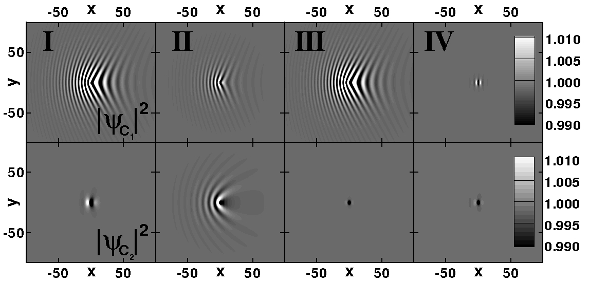
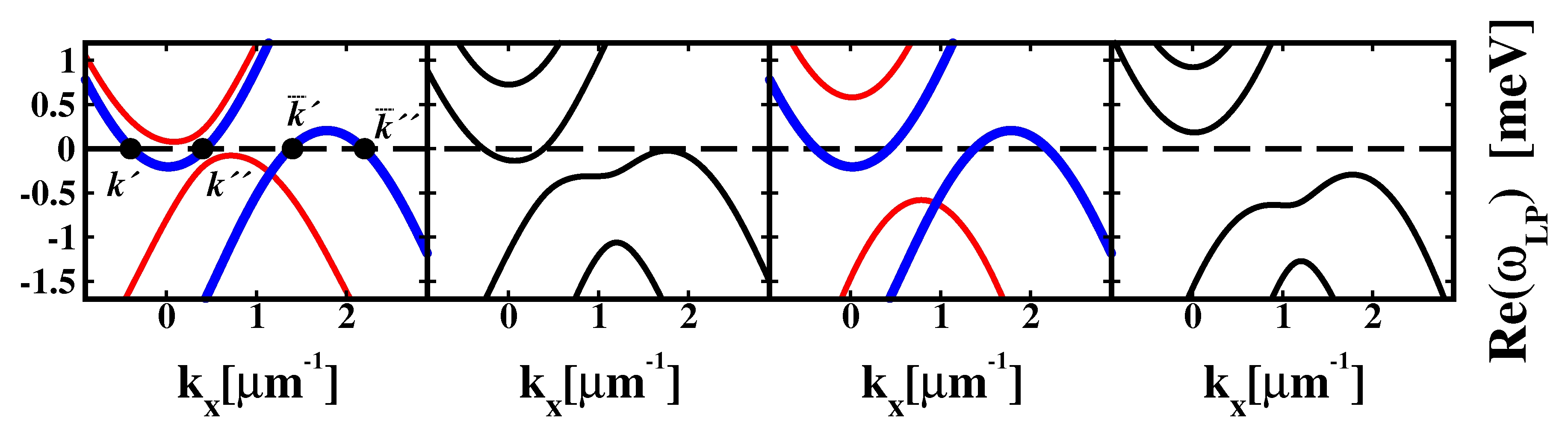
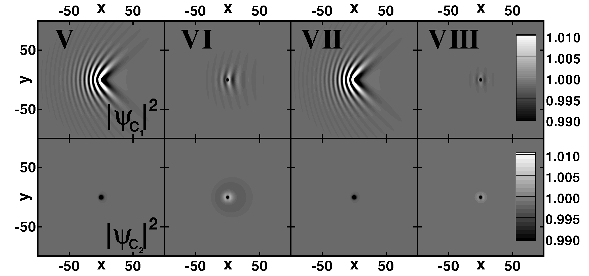
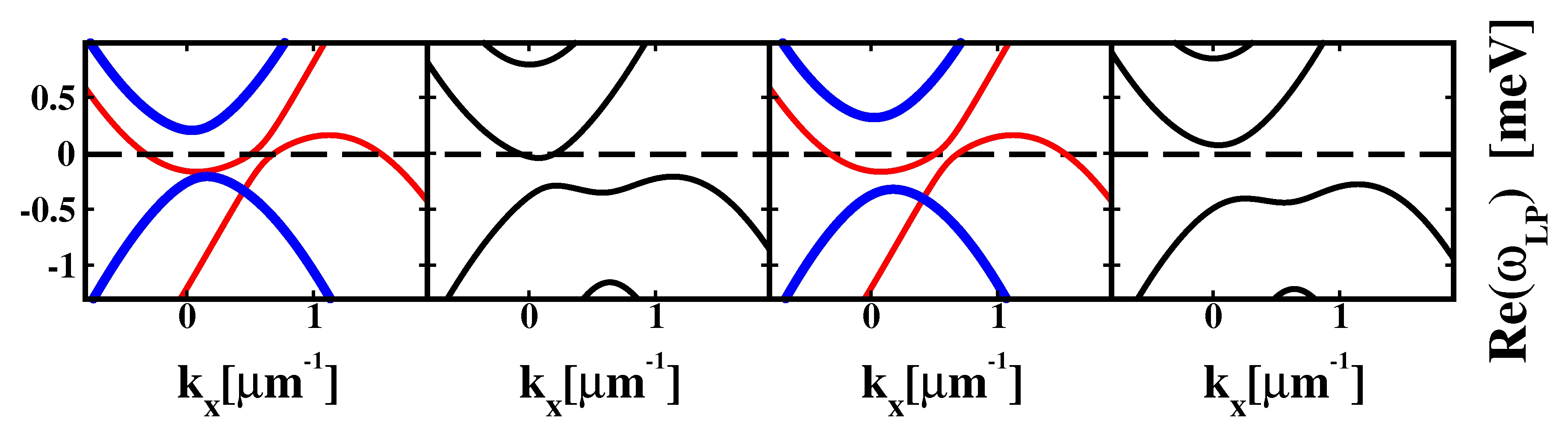
Figure 1: (Color online) 2D contour plots of the space profiles $|\psi_{{1,2}_{C}}({\mathbf{r}})|^{2}$ [arbitrary units] (gray maps) and associated excitation spectra $\Re[\omega_{LP}({\mathbf{k}})]$ [meV]: the two laser pumps are shined at momenta $k_{1}=0.9$ and $k_{2}=0.4~{}\mu$m^-1 (columns I-IV) and at momenta $k_{1}=0.6$ and $k_{2}=0.1~{}\mu$m^-1 (columns V-VIII), while in all cases the laser energies are $0.5$ meV blue-detuned above the bare LP branch ($\kappa_{C}=\kappa_{X}=0.1$ meV). Columns I, III, V, and VII corresponds to the case where fluid 1 (red) is uncoupled from fluid 2 (blue), while columns II, IV, VI, and VIII describe the coupled cases. The densities of the two components have been fixed to $g_{X}|\psi_{1_{X}}|^{2}=1.5$ meV and $g_{X}|\psi_{2_{X}}|^{2}=1.2$ meV (columns I and II), to $g_{X}|\psi_{1_{X}}|^{2}=1.5$ meV and $g_{X}|\psi_{2_{X}}|^{2}=2.5$ meV (III and IV), to $g_{X}|\psi_{1_{X}}|^{2}=1.0$ meV and $g_{X}|\psi_{2_{X}}|^{2}=1.25$ meV (V and VI), and to $g_{X}|\psi_{1_{X}}|^{2}=1.0$ meV and $g_{X}|\psi_{2_{X}}|^{2}=1.5$ meV (VII and VIII). The momentum labels $k^{\prime}=-0.4$, $k^{\prime\prime}=0.40$, $\bar{k}^{\prime}=1.4$ and $\bar{k}^{\prime\prime}=2.2~{}\mu$m^-1 are explicitly indicated in the spectrum of column I.

The SP vs. SB character of the excitations generated by the defect potential can be studied by analyzing the real part of the Bogoliubov spectra $\omega_{LP_{j},UP_{j}}^{\pm}({\mathbf{k}})$. According to the Landau criterion for superfluidity, a fluid moving against a defect is in a SB regime if it is unable to excite quasi particle states (i.e., when elastic scattering is forbidden). This happens when the system’s excitation spectra, is either gapped, i.e.,

$$\Re[\omega_{LP_{j}}^{\pm}({\mathbf{k}})]\neq 0\quad\forall{\mathbf{k}}\,,$$ (3)

or it satisfies the condition $\Re[\omega_{LP_{j}}^{\pm}({\mathbf{k}}_{0})]=0$ for one value of the momentum only, namely that of the condensate’s momentum ${\mathbf{k}}_{0}$ (linear spectrum). Conversely, when for at least two values of ${\mathbf{k}}$, $\Re[\omega_{LP_{j}}^{\pm}({\mathbf{k}})]=0$, the system is in the SP regime. Note that, unlike for superfluid systems in thermal equilibrium, for polaritons the above definition of the SB regime does not mean a complete suppression of the energy dissipation into the creation of quasi particles Wouters and Carusotto (2010a); Cancellieri et al. (2010). In fact, because of the polariton finite lifetime, the spectra are broadened and a residual drag is always present.

In order to analyze the superfluid properties of the system, in Fig. 1 we compare the cases of coupled and uncoupled fluids. This can be regarded, both from a theoretical and experimental point of view, as the comparison between the case of two fluids pumped in different regions of the cavity (uncoupled) with the case of two fluids pumped in the same region (coupled). Clearly, the densities of two coupled fluids depend on both pump intensities, and thus, in order to correctly compare the coupled and uncoupled scenarios, such intensities must be adjusted so that the polariton densities of each fluid in the coupled case separately coincide with the ones of the uncoupled fluids. Typical behaviors of the system are illustrated in Fig. 1, where both 2D contour plots of the space profiles $|\psi_{{1,2}_{C}}({\mathbf{r}})|^{2}$ and their associated excitation spectra $\Re[\omega_{LP}({\mathbf{k}})]$ are plotted. Let us consider first the case of the panels corresponding to columns I to IV: for uncoupled components (columns I and III), the spectrum of fluid $1$ (red) crosses the zero-energy line in four points at $k^{\prime}$, $k^{\prime\prime}$, $\bar{k}^{\prime}$ and $\bar{k}^{\prime\prime}$, satisfying $k^{\prime}+\bar{k}^{\prime\prime}=2k_{1}$ and $k^{\prime\prime}+\bar{k}^{\prime}=2k_{1}$. Two quasi particles with momentum $k_{1}$ can be excited, and thus fluid $1$ is in the SP regime. Now Cherenkov-like waves can be emitted from the $\delta$-like defect positioned in ${\mathbf{r}}=0$ (see the $|\psi_{{1}_{C}}({\mathbf{r}})|^{2}$ map of column I). In contrast, the spectrum of the fluid $2$ (blue) is gapped, no Cherenkov waves can be emitted from the defect, and therefore fluid $2$ is in the SB regime. When, instead, we analyze the case where the same two fluids are coupled (column II), we see that Cherenkov-like waves appear in the 2D profiles of both $|\psi_{C_{1}}({\mathbf{r}})|^{2}$ and $|\psi_{C_{2}}({\mathbf{r}})|^{2}$. This is because the interaction between the two fluids produces an anticrossing, and thus a mixing, of the corresponding Bogoliubov modes. As a consequence, the fluid injected in the component $2$ can now scatter against the defect. An opposite case is shown in columns III and IV. The polariton density of fluid $2$ is now doubled with respect to the case of columns I and II, keeping unchanged the fluid $1$ density. Now, the effect of the coupling is to considerably decrease the scattering in component $1$ and the coupled excitation spectra satisfies Eq. (3): in this case the effect of the coupling is that both components can flow without friction. From this analysis, we can conclude that a two-component polariton fluid can be in SB regime only if both components are SB. This is because, due to the coupling, the Bogoliubov spectra mix and only the scattering properties of the system as a whole can be defined. Since the combined state of the coupled system depends on the densities of both fluids, the system as a whole is SP or SB depending on which component dominates. In addition, we find that when a fluid has either a too low density or a too high velocity to exhibit frictionless flow on its own, the fluid can instead flow without friction when coupled to another fluid with the suitable properties. In order to identify the role played by the coupling strength between the two fluids in our predictions, we consider in columns V-VIII of Fig. 1 the case of two fluids with a higher photonic component, and therefore more weakly coupled, with respect to the case of columns I-IV. While the same qualitative conclusions hold, the scattering induced by fluid $1$ over fluid $2$ is now substantially smaller and comparable with the effect due to the polariton linewidth.

Figure 2: (Color online) Phase diagram, as a function of the rescaled pump intensities $\sqrt{g_{X}}F_{1,2}$ [meV^3/2], showing the regions where the system is SP (red) or SB (blue). In this case, the two lasers pump at an energy $0.5$ meV blue-detuned from the bare LP branch and $\kappa_{X}=\kappa_{C}=0.1$ meV. In panel I, the lasers momenta are $k_{1}=0.6$, and $k_{2}=0.1~{}\mu$m^-1. In panels II and III the $x$-component of the momentum of laser 2 is increased by $0.2$ and $0.4~{}\mu$m^-1 respectively. Points $A$ and $B$ correspond to cases discussed in the text.

Applying Eq. (3), one can study the SP and SB character of the binary fluid as a function of the two particle densities (see Supplemental Material). It is however useful to perform this study also as a function of the two pump intensities, being these the experimentally accessible parameters. Panels I-III of Fig. 2 show the SB regions for three values of the fluid $2$ velocity. Clearly, if any of the two pumps is switched off ($F_{j}=0$), one reproduces the single-fluid case. As $k_{2}<k_{1}$, the SB region for $F_{1}=0$ starts at lower pump intensities than the SB region for $F_{2}=0$ (panel I): for higher fluid velocities, the system requires higher polariton populations, and therefore higher pump intensities, in order to be in the SB regime. Even if the analytical dependence of the SB region on the two pump intensities cannot be evaluated, one can qualitatively understand its behavior: for fixed cavity and laser parameters, the SB regime depends on the total particle density seen by the two components $|\psi_{X}^{ss}|^{2}=|\psi_{1_{X}}^{ss}|^{2}+|\psi_{2_{X}}^{ss}|^{2}$. For $F_{2}=0$ and $\sqrt{g_{X}}F_{1}=0.45$ meV^3/2 (point A of Fig. 2), the total particle density $|\psi_{X}^{ss}|^{2}$, seen by the fluid is $|\psi_{X}^{ss}|^{2}=|\psi_{1_{X}}|^{2}=1.37$ meV/$g_{X}$ and the system is SB. If now the second pump is turned on and $\sqrt{g_{X}}F_{2}$ set to $0.3$ meV^3/2 (point B), the total particle density decreases to $|\psi_{X}^{ss}|^{2}=1.34$ meV/$g_{X}$ and the system is in the SP regime. This is because when $F_{2}$ is turned on the particle density increases by a factor $|\psi_{2_{X}}|^{2}$ but, at the same time, the fluid $1$ particle density is decreased by a bigger factor. Since the system starts in a SB regime, the dressed LP branch is blue-detuned with respect to the pump frequency $\omega_{1}$ and, therefore, the effect of $F_{2}\neq 0$ is to further bluedetune it, making it more difficult for pump 1 to fill the cavity.

Evaluating the linear spectrum of excitations in experiments can be a challenging task. In principle, the appearance and disappearance of Cherenkov waves could be used to determine the SP to SB crossover, similarly to Ref. Amo et al. (2009). However, for a quantitative description of the crossover we propose to determine the drag force exerted by the binary fluid on the defect $V_{C}({\mathbf{r}})$ Wouters and Carusotto (2010a); Astrakharchik and Pitaevskii (2004); Cancellieri et al. (2010):

$${\mathbf{F}}_{d}=\frac{1}{\int d{\mathbf{r}}|\psi_{C}({\mathbf{r}})|^{2}}\int d{\mathbf{r}}|\psi_{C}({\mathbf{r}})|^{2}\nabla V_{C}({\mathbf{r}})\;.$$ (4)

We evaluate the time average of the cavity field $\psi_{C}({\mathbf{r}})$, numerically solving the dynamics of Eq. (1) on a 2D grid ($256\times 256$ points) of $150\times 150~{}\mu$m, by using a fifth-order adaptive-step Runge-Kutta algorithm. The pumping lasers have a smoothen top-hat spatial profile ${\cal F}_{1,2}({\bf r})$ with a full width at half maximum of $\sigma=130~{}\mu$m; the weak defect has a Gaussian shape. In Fig. 3 we plot the drag force that the binary fluid exerts on the defect as a function of the two fluid numbers of particles, comparing the coupled and uncoupled cases. The limit when one of the two pumps is turned off recovers the results for a single fluid Cancellieri et al. (2010): when the particle density increases, the drag force decreases from high values to a residual finite value. For the case with two currents, we find that the drag force exerted by two coupled fluids on the defect is weaker than the drag force exerted by the two uncoupled components. This is because, in the coupled case, particles of each component move in an effectively denser medium than in the uncoupled case (Eq. (3) of the Supplemental Material), thus the drag force is smaller. From the experimental point of view, in order to determine the drag force, one could measure the near-field cavity emission in a region around the defect as a function of position, and, if the shape of the defect is known, one could evaluate the drag force making use of Eq. (4). Note, that the important quantity needed for this measure is the shape of the potential, not its precise height. Any uncertainty in the defect potential intensity will systematically affect the drag force overall scale but not its global dependence on the polariton densities. Finally, we would like to stress that higher fluid velocities and shorter polariton lifetimes give rise to higher values (therefore more easily measurable) of the drag force and of its residual value at high polariton density.

Figure 3: (Color online) Time average of the drag force of the fluid as a function of the number of particles $N_{1}$ and $N_{2}$. The two lasers are pumping at momenta $k_{1}=0.9$, and $k_{2}=1.0~{}\mu$m^-1 and energies $0.3$ meV blue-detuned from the bare LP branch, and $\kappa_{X}=0.22$ meV, $\kappa_{C}=0.22$ meV. Red dots correspond to the case of two uncoupled fluids, while black cubes correspond to the case of coupled fluids. The drag force for the uncoupled case is evaluated as: ${\mathbf{F}}_{d}=\frac{1}{N_{1}+N_{2}}(N_{1}{\mathbf{F}}_{d_{1}}+N_{2}{\mathbf{F}}_{d_{2}})$.

To conclude, we would like to note that we can draw this Letter’s conclusions independently on the polariton lifetime, as they exclusively depend on the real part of the Bogoliubov spectra and therefore hold in equilibrium conditions, e.g., for the case of atomic superfluids. However, even for extremely long polariton lifetimes, binary polariton superfluids are more general than atomic ones. This is because, while for the latter case the chemical potential fixes the atom density, for the former, the laser frequency can be tuned independently on its power which determines the polariton density. Further, the polariton dispersion deviates from quadratic at large momenta. This together with the finite polariton lifetime has important consequences on the Bogoliubov spectrum, even in the case of one fluid only: while for atoms, Bogoliubov spectra are all linear at small wave vectors, for coherently pumped polaritons they can in addition be gapped or diffusive Ciuti and Carusotto (2005).

This research has been supported by the Spanish MEC (MAT2008-01555, QOIT-CSD2006-00019) and CAM (S-2009/ESP-1503). F.M.M. acknowledges the financial support from the program Ramón y Cajal.

Frictionless flow in a binary polariton superfluid: Supplementary Material

I Appendix A

I.1 Stationary solutions in the homogeneous case

We describe the system of resonantly-driven microcavity polaritons via Gross-Pitaevskii equation for coupled cavity ($\psi_{C}$) and exciton ($\psi_{X}$) fields generalized to include the description of the finite life-time of photons and excitons and the injection of polaritons in the cavity through resonant pumping ($\hbar=1$) Whittaker (2005):

$$i\partial_{t}\begin{pmatrix}\psi_{X}\\ \psi_{C}\end{pmatrix}=\begin{pmatrix}0\\ F\end{pmatrix}+\left[\hat{H}_{0}+\begin{pmatrix}g_{X}|\psi_{X}|^{2}+V_{X}&0\\ 0&V_{C}\end{pmatrix}\right]\begin{pmatrix}\psi_{X}\\ \psi_{C}\end{pmatrix}\\$$

$$\hat{H}_{0}=\begin{pmatrix}\omega_{X}-i\kappa_{X}&\Omega_{R}/2\\ \Omega_{R}/2&\omega_{C}(-i\nabla)-i\kappa_{C}\end{pmatrix}\;.$$ (5)

Polaritons are continuously injected into the cavity by two spatially homogeneous continuous-wave laser fields:

$$F({\mathbf{r}},t)=F_{1}e^{i({\mathbf{k}}_{1}\cdot{\mathbf{r}}-\omega_{1}t)}+F_{2}e^{i({\mathbf{k}}_{2}\cdot{\mathbf{r}}-\omega_{2}t)}\;,$$

with intensities $F_{1,2}$, and with independently tunable frequencies $\omega_{1,2}$ and momenta ${\mathbf{k}}_{1,2}$, which can be experimentally changed by changing the laser angle of incidence with respect to the growth direction. Under the continuous pump conditions and in the homogeneous case (i.e., in absence of an external potential, $V_{C,X}({\mathbf{r}})=0$), the mean-field solutions of Eq. (5) can be written as:

$$\psi_{X,C}({\mathbf{r}},t)=\psi^{ss}_{1_{X,C}}e^{i({\mathbf{k}}_{1}\cdot{\mathbf{r}}-\omega_{1}t)}+\psi^{ss}_{2_{X,C}}e^{i({\mathbf{k}}_{2}\cdot{\mathbf{r}}-\omega_{2}t)}\;.$$ (6)

Substituting the expression (6) into (5) we obtain 4 contributions, two of which oscillate at the main frequencies $\omega_{1}$ and $\omega_{2}$ and the additional two at the replica (or satellite state) frequencies $\omega_{1}-\Delta\omega$ and $\omega_{2}+\Delta\omega$, where $\Delta\omega=\omega_{2}-\omega_{1}$. Similarly to what is done in the OPO regime Whittaker (2005); Wouters and Carusotto (2007) where replica states in addition to the pump signal and idler states are neglected, here, we consider only the terms oscillating at the main frequencies $\omega_{1}$ and $\omega_{2}$. In this approximation the mean-field values for $\psi^{ss}_{{1,2}_{X,C}}$, can be obtained solving the following system of complex equations:

$$\begin{cases}[\omega_{X}-\omega_{1}-i\kappa_{X}+G_{12}]\psi_{1_{X}}^{ss}+\frac{\Omega_{R}}{2}\psi_{1_{C}}^{ss}=0\\ [\omega_{C}({\bf k}_{1})-\omega_{1}-i\kappa_{C}]\psi_{1_{C}}^{ss}+\frac{\Omega_{R}}{2}\psi_{1_{X}}^{ss}+F_{1}=0\\ [\omega_{X}-\omega_{2}-i\kappa_{X}+G_{21}]\psi_{2_{X}}^{ss}+\frac{\Omega_{R}}{2}\psi_{2_{C}}^{ss}=0\\ [\omega_{C}({\bf k}_{2})-\omega_{2}-i\kappa_{C}]\psi_{2_{C}}^{ss}+\frac{\Omega_{R}}{2}\psi_{2_{X}}^{ss}+F_{2}=0\;,\end{cases}$$ (7)

where $G_{ij}=g_{X}(|\psi_{i_{X}}^{ss}|^{2}+2|\psi_{j_{X}}^{ss}|^{2})$ with $i\neq j=1,2$. The mean-field system of equations (7) can have up to 9 solutions, i.e. 6 solutions more than in the case of one pumping laser, but only a maximum of 3 solutions are stable. For details see Ref. Cancellieri et al. (2011).

I.2 Linearized Bogoliubov-like theory

The perturbative Bogoliubov-like analysis, first introduced for resonantly pumped polaritons in Refs. Carusotto and Ciuti (2004); Ciuti and Carusotto (2005), is here generalized to the case of two pumping lasers. Adding small fluctuations to the homogeneous solution, the Bogoliubov-like theory allows for the study of the dynamical stability of the two-pump-frequency mean-field solution, as well as for the study of the subsonic or supersonic character of the fluid. Moreover, the Bogoliubov theory allows for the evaluation of the real and momentum space representation of the photonic and excitonic distributions in the presence of weak perturbing potentials. We start our analysis by adding small fluctuations ($\theta_{1,2_{X,C}}$) to the homogeneous solutions:

$$\psi_{X,C}({\mathbf{r}},t)=e^{-i\omega_{1}t}\left[e^{i{\mathbf{k}}_{1}\cdot{\mathbf{r}}}\psi^{ss}_{1_{X,C}}+\theta_{1_{X,C}}({\mathbf{r},t})\right]+e^{-i\omega_{2}t}\left[e^{i{\mathbf{k}}_{2}\cdot{\mathbf{r}}}\psi^{ss}_{2_{X,C}}+\theta_{2_{X,C}}({\mathbf{r},t})\right]\;,$$ (8)

where the fluctuation fields can be divided into particle-like and hole-like excitations:

$$\theta_{i_{X,C}}({\mathbf{r}},t)=\sum_{{\mathbf{k}}}[e^{-i\omega t+i{\mathbf{k}}\cdot{\mathbf{r}}}u_{i_{X,C}{\mathbf{k}}}+e^{i\omega t+i(2{\mathbf{k}}_{i}-{\mathbf{k}})\cdot{\mathbf{r}}}v^{*}_{i_{X,C}{\mathbf{k}}}]\;.$$

Inserting Eq. (8) in Eq. (5) and expanding up to linear terms in $\theta_{1,2_{X,C}}$, we obtain 4 terms oscillating at frequencies $\omega_{1}-\Delta\omega\pm\omega$ and $\omega_{2}+\Delta\omega\pm\omega$, which we neglect, and 4 terms oscillating at $\omega_{1,2}\pm\omega$ which we consider. In other words, we limit our study to the case where only the two states with frequencies $\omega_{1,2}$ are occupied and analyze the excitation of particles with frequencies $\omega_{1,2}\pm\omega$.

I.2.1 Excitation Spectra

Within this analysis, the stability of the system and the scattering properties of the collective excitations are evaluated through the spectra of the particle-like $u_{i_{X,C}{\mathbf{k}}}$ and of the hole-like $v^{*}_{i_{X,C}{\mathbf{k}}}$ excitations which are given by the solutions of the eigenvalue equation:

$$\left[\omega\mathbb{I}-\mathbb{L}_{{\mathbf{k}}}\right]\mathbb{U}_{{\mathbf{k}}}=\left[\omega\mathbb{I}-\begin{pmatrix}\mathbb{L}_{11{\mathbf{k}}}&\mathbb{L}_{12{\mathbf{k}}}\\ \mathbb{L}_{21{\mathbf{k}}}&\mathbb{L}_{22{\mathbf{k}}}\end{pmatrix}\right]\mathbb{U}_{{\mathbf{k}}}=0\;,$$ (9)

where the excitation fields have been arranged in the 8-component vector $\mathbb{U}^{\text{T}}=(u_{1_{X}},u_{1_{C}},v_{1_{X}},v_{1_{C}},u_{2_{X}},u_{2_{C}},v_{2_{X}},v_{2_{C}})$. In the above equation the matrices $\mathbb{L}_{ij{\mathbf{k}}}$ with $i\neq j$ are given by

$$2g_{X}e^{i({\mathbf{k}}_{i}-{\mathbf{k}}_{j})\cdot{\mathbf{r}}}\begin{pmatrix}\psi_{i_{X}}^{ss}\psi_{j_{X}}^{ss\star}&0&\psi_{i_{X}}^{ss}\psi_{j_{X}}^{ss}&0\\ 0&0&0&0\\ -\psi_{i_{X}}^{ss\star}\psi_{j_{X}}^{ss\star}&0&-\psi_{i_{X}}^{ss\star}\psi_{j_{X}}^{ss}&0\\ 0&0&0&0\end{pmatrix}$$

and $\mathbb{L}_{jj{\mathbf{k}}}$ are given by

$$\begin{pmatrix}\omega_{X}-\omega_{j}-i\kappa_{X}+2g_{X}|\psi_{X}^{ss}|^{2}&\frac{\Omega_{R}}{2}&g_{X}\psi_{j_{X}}^{ss}\psi_{j_{X}}^{ss}&0\\ \frac{\Omega_{R}}{2}&\omega_{C}({\mathbf{k}})-\omega_{j}-i\kappa_{C}&0&0\\ -g_{X}\psi_{j_{X}}^{ss\star}\psi_{j_{X}}^{ss\star}&0&-\omega_{X}(2{\mathbf{k}}_{j}-{\mathbf{k}})+\omega_{j}-i\kappa_{X}-2g_{X}|\psi_{X}^{ss}|^{2}&-\frac{\Omega_{R}}{2}\\ 0&0&-\frac{\Omega_{R}}{2}&-\omega_{C}(2{\mathbf{k}}_{j}-{\mathbf{k}})+\omega_{j}-i\kappa_{C}\end{pmatrix}\;,$$

with $|\psi_{X}^{ss}|^{2}=|\psi_{1_{X}}^{ss}|^{2}+|\psi_{2_{X}}^{ss}|^{2}$ being the total excitonic density. At given values of the pumping strength $F_{1}$ and $F_{2}$, the solutions of the mean-field equations (7) are stable if all the eight eigenvalues $\omega_{LP_{j},UP_{j}}^{\pm}({\mathbf{k}})$ of Eq. (9) have negative imaginary part for every value of the momentum ${\mathbf{k}}$. When the stability of the solution for given values of the pump intensities has been checked, the information about the scattering properties of the fluctuations can be extracted by the analysis of the real part of the eight eigenvalues.

I.2.2 Response to a weak potential

We evaluate now the response of the excitonic and photonic density profiles to a weak static potential $V_{C}({\mathbf{r}})$. The starting point is the equation of motion for the fluctuation fields in the presence of a perturbation Ciuti and Carusotto (2005): $i\partial_{t}\mathbb{U}_{{\mathbf{k}}}=\mathbb{L}_{{\mathbf{k}}}\mathbb{U}_{{\mathbf{k}}}+\mathbb{P}_{{\mathbf{k}}}$, where

$$\mathbb{P}_{{\mathbf{k}}}=\begin{pmatrix}\tilde{V}_{X}({\mathbf{k}})\psi_{1_{X}}^{ss}\\ \tilde{V}_{C}({\mathbf{k}})\psi_{1_{C}}^{ss}\\ -\tilde{V}_{X}({\mathbf{k}}-2{\mathbf{k}}_{1})\psi_{1_{X}}^{*ss}\\ -\tilde{V}_{C}({\mathbf{k}}-2{\mathbf{k}}_{1})\psi_{1_{C}}^{*ss}\\ \tilde{V}_{X}({\mathbf{k}})\psi_{2_{X}}^{ss}\\ \tilde{V}_{C}({\mathbf{k}})\psi_{2_{C}}^{ss}\\ -\tilde{V}_{X}({\mathbf{k}}-2{\mathbf{k}}_{2})\psi_{2_{X}}^{*ss}\\ -\tilde{V}_{C}({\mathbf{k}}-2{\mathbf{k}}_{2})\psi_{2_{C}}^{*ss}\\ \end{pmatrix}\;,$$ (10)

where $\tilde{V}_{C,X}({\mathbf{k}})$ is the Fourier transform into momentum space of $V_{C,X}({\mathbf{r}})$. Since we are interested in the steady state of the system we can extract the perturbed photonic and excitonic fields in momentum space as:

$$\mathbb{U}_{{\mathbf{k}}}=-\mathbb{L}^{-1}_{{\mathbf{k}}}\mathbb{P}_{{\mathbf{k}}}\;,$$ (11)

and back-Fourier transform them in order to obtain the perturbation fields in real space. At this point, the total photon/exciton field intensity for each component (homogeneous solution + potential induced perturbation), normalized to the intensity of the homogeneous solution without the potential is obtained as:

$$|\psi_{i_{C,X}}|^{2}=\frac{|\psi^{ss}_{i_{C,X}}+\theta_{i_{X,C}}({\mathbf{r}},t)|^{2}}{|\psi^{ss}_{i_{C,X}}|^{2}}\;.$$ (12)

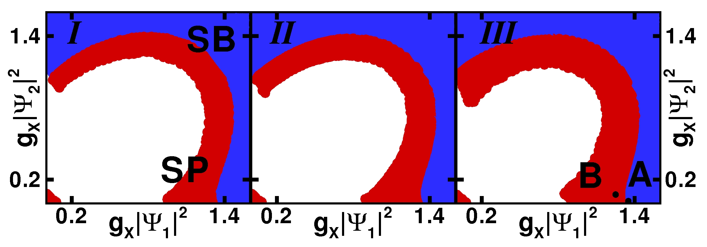
Figure 4: (Color online) Phase diagram, as a function of $g_{X}|\psi_{i_{X}}|^{2}$ [meV], showing the regions where the system is SP (red) or SB (blue). The white regions correspond do particle densities for which the system is not stable. In this case, the two lasers pump at an energy $0.5$ meV blue detuned from the bare LP branch and $\kappa_{X}=\kappa_{C}=0.1$ meV. In Panel $I$, the lasers momenta are $k_{1}=0.6$, and $k_{2}=0.1~{}\mu$m^-1. In Panels $II$ and $III$ the $x$-component of the momentum of laser 2 is increased by $0.2$ and $0.4~{}\mu$m^-1 respectively. The points $A$ and $B$ correspond to cases discussed in the text.

II Appendix B

II.1 Phase diagram for the sub (super) sonic behavior of a binary fluid

Looking at the spectra of small excitations over the stationary state, it is possible to determine the sub-sonic (SB) or super-sonic (SP) behavior of the coupled binary fluid. For given values of the lasers and cavity parameters, it is possible to evaluate the stability of the system and, for the stable conditions, the existence of a SB solution. As discussed in the article, if the real part of the excitation spectra satisfies the condition:

$$\Re[\omega_{LP_{j}}^{\pm}({\mathbf{k}})]\neq 0\quad\forall{\mathbf{k}}\,,$$ (13)

the fluid is considered to be SB. In Fig. 4 we plot the stable solutions that are SB (blue) or SP (red) as a function of the particle densities of the two modes $|\psi_{i_{X}}|^{2}$. The three panels reproduce the same laser and cavity conditions as panels $I-III$ of Fig. 2 of the article. In the case of one pump turned off (for example $F_{2}$, i.e. $|\psi_{2_{X}}|^{2}=0$) we have a SP region at low densities, a wide region for which the system is not stable (in white), a second SP region and, finally, a SB one that starts at $g_{X}|\psi_{1_{X}}|^{2}=1.36$. In Panel $III$ we show the two points $A$ and $B$ as in the article. Point $A$ is in the SB region while point $B$ is in the SP one. Note, that the boundary between the SB and the SP region is not perfectly circular meaning that the SB behavior depends on the two densities but in an unbalanced way. This can be understood recalling that polaritons at different energies and momenta have different masses and couplings, and therefore their weight on the SB behavior is different.

References

- Pitaevskii and Stringari (2003) L. P. Pitaevskii and S. Stringari, Bose-Einstein Condensation (Clarendon Press, Oxford, 2003).
- Berloff (2005) N. G. Berloff, Phys. Rev. Lett. 94, 120401 (2005).
- Susanto et al. (2007) H. Susanto et al., Phys. Rev. A 75, 055601 (2007).
- Kravchenko and Fil (2008) L. Kravchenko and D. Fil, Journal of Low Temperature Physics 150 (2008).
- Carusotto and Ciuti (2004) I. Carusotto and C. Ciuti, Phys. Rev. Lett. 93, 166401 (2004).
- Ciuti and Carusotto (2005) C. Ciuti and I. Carusotto, physica status solidi (b) 242, 2224 (2005), ISSN 1521-3951.
- Amo et al. (2009) A. Amo et al., Nat. Phys. 5, 805 (2009).
- Cancellieri et al. (2010) E. Cancellieri, F. M. Marchetti, M. H. Szymańska, and C. Tejedor, Phys. Rev. B 82, 224512 (2010).
- Amo et al. (2008) A. Amo et al., Nature 457, 291 (2008).
- Sanvitto et al. (2010) D. Sanvitto et al., Nature Physics 6, 527 (2010), eprint 0907.2371.
- Marchetti et al. (2010) F. M. Marchetti, M. H. Szymańska, C. Tejedor, and D. M. Whittaker, Phys. Rev. Lett. 105, 063902 (2010).
- El et al. (2007) G. A. El et al., J. Phys. A 40, 611 (2007),
- Whittaker (2005) D. M. Whittaker, Phys. Rev. B 71, 115301 (2005).
- Amo et al. (2010) A. Amo et al., Phys. Rev. B 82, 081301 (2010).
- Cancellieri et al. (2011) E. Cancellieri, F. M. Marchetti, M. H. Szymańska, and C. Tejedor, Phys. Rev. B 83, 214507 (2011).
- Wouters and Carusotto (2010a) M. Wouters and I. Carusotto, Phys. Rev. Lett. 105, 020602 (2010a).
- Astrakharchik and Pitaevskii (2004) G. E. Astrakharchik and L. P. Pitaevskii, Phys. Rev. A 70, 013608 (2004).
- Wouters and Carusotto (2007) M. Wouters and I. Carusotto, Phys. Rev. Lett. 99, 140402 (2007).