Multi-task Regression using Minimal Penalties

Abstract

In this paper we study the kernel multiple ridge regression framework, which we refer to as multi-task regression, using penalization techniques. The theoretical analysis of this problem shows that the key element appearing for an optimal calibration is the covariance matrix of the noise between the different tasks. We present a new algorithm to estimate this covariance matrix, based on the concept of minimal penalty, which was previously used in the single-task regression framework to estimate the variance of the noise. We show, in a non-asymptotic setting and under mild assumptions on the target function, that this estimator converges towards the covariance matrix. Then plugging this estimator into the corresponding ideal penalty leads to an oracle inequality. We illustrate the behavior of our algorithm on synthetic examples.

Keywords: multi-task, oracle inequality, learning theory

1 Introduction

A classical paradigm in statistics is that increasing the sample size (that is, the number of observations) improves the performance of the estimators. However, in some cases it may be impossible to increase the sample size, for instance because of experimental limitations. Hopefully, in many situations practicioners can find many related and similar problems, and might use these problems as if more observations were available for the initial problem. The techniques using this heuristic are called “multi-task” techniques. In this paper we study the kernel ridge regression procedure in a multi-task framework.

One-dimensional kernel ridge regression, which we refer to as “single-task” regression, has been widely studied. As we briefly review in Section 3 one has, given $n$ data points $(X_{i},Y_{i})_{i=1}^{n}$, to estimate a function $f$, often the conditional expectation $f(X_{i})=\mathbb{E}[Y_{i}|X_{i}]$, by minimizing the quadratic risk of the estimator regularized by a certain norm. A practically important task is to calibrate a regularization parameter, that is, to estimate the regularization parameter directly from data. For kernel ridge regression (a.k.a. smoothing splines), many methods have been proposed based on different principles, for example, Bayesian criteria through a Gaussian process interpretation (see, e.g., Rasmussen and Williams, 2006) or generalized cross-validation (see, e.g., Wahba, 1990). In this paper, we focus on the concept of minimal penalty, which was first introduced by Birgé and Massart (2007) and Arlot and Massart (2009) for model selection, then extended to linear estimators such as kernel ridge regression by Arlot and Bach (2011).

In this article we consider $p\geq 2$ different (but related) regression tasks, a framework we refer to as “multi-task” regression. This setting has already been studied in different papers. Some empirically show that it can lead to performance improvement (Thrun and O’Sullivan, 1996; Caruana, 1997; Bakker and Heskes, 2003). Liang et al. (2010) also obtained a theoretical criterion (unfortunately non observable) which tells when this phenomenon asymptotically occurs. Several different paths have been followed to deal with this setting. Some consider a setting where $p\gg n$, and formulate a sparsity assumption which enables to use the group Lasso, assuming all the different functions have a small set of common active covariates (see for instance Obozinski et al., 2011; Lounici et al., 2010). We exclude this setting from our analysis, because of the Hilbertian nature of our problem, and thus will not consider the similarity between the tasks in terms of sparsity, but rather in terms of an Euclidean similarity. Another theoretical approach has also been taken (see for example, Brown and Zidek (1980), Evgeniou et al. (2005) or Ando and Zhang (2005) on semi-supervised learning), the authors often defining a theoretical framework where the multi-task problem can easily be expressed, and where sometimes solutions can be computed. The main remaining theoretical problem is the calibration of a matricial parameter $M$ (typically of size $p$), which characterizes the relationship between the tasks and extends the regularization parameter from single-task regression. Because of the high dimensional nature of the problem (i.e., the small number of training observations) usual techniques, like cross-validation, are not likely to succeed. Argyriou et al. (2008) have a similar approach to ours, but solve this problem by adding a convex constraint to the matrix, which will be discussed at the end of Section 5.

Through a penalization technique we show in Section 2 that the only element we have to estimate is the correlation matrix $\Sigma$ of the noise between the tasks. We give here a new algorithm to estimate $\Sigma$, and show that the estimation is sharp enough to derive an oracle inequality for the estimation of the task similarity matrix $M$, both with high probability and in expectation. Finally we give some simulation experiment results and show that our technique correctly deals with the multi-task settings with a low sample-size.

1.1 Notations

We now introduce some notations, which will be used throughout the article.

• The integer $n$ is the sample size, the integer $p$ is the number of tasks.

• For any $n\times p$ matrix $Y$, we define

  $$y=\operatorname{vec}(Y):=\left(Y_{1,1},\ldots,Y_{n,1},Y_{1,2},\ldots,Y_{n,2},\ldots,Y_{1,p},\ldots,Y_{n,p}\right)\in\mathbb{R}^{np},$$

  that is, the vector in which the columns $Y^{j}:=(Y_{i,j})_{1\leq i\leq n}$ are stacked.

• $\mathcal{M}_{n}(\mathbb{R})$ is the set of all matrices of size $n$.

• $\mathcal{S}_{p}(\mathbb{R})$ is the set of symmetric matrices of size $p$.

• $\mathcal{S}_{p}^{+}(\mathbb{R})$ is the set of symmetric positive-semidefinite matrices of size $p$.

• $\mathcal{S}_{p}^{++}(\mathbb{R})$ is the set of symmetric positive-definite matrices of size $p$.

• $\preceq$ denotes the partial ordering on $\mathcal{S}_{p}(\mathbb{R})$ defined by: $A\preceq B$ if and only if $B-A\in\mathcal{S}_{p}^{+}(\mathbb{R})$.

• $\mathbf{1}$ is the vector of size $p$ whose components are all equal to $1$.

• $\left\|\cdot\right\|_{2}$ is the usual Euclidean norm on $\mathbb{R}^{k}$ for any $k\in\mathbb{N}$: $\forall u\in\mathbb{R}^{k}$, $\left\|u\right\|_{2}^{2}:=\sum_{i=1}^{k}u_{i}^{2}$.

2 Multi-task Regression: Problem Set-up

We consider $p$ kernel ridge regression tasks. Treating them simultaneously and sharing their common structure (e.g., being close in some metric space) will help in reducing the overall prediction error.

2.1 Multi-task with a Fixed Kernel

Let $\mathcal{X}$ be some set and $\mathcal{F}$ a set of real-valued functions over $\mathcal{X}$. We suppose $\mathcal{F}$ has a reproducing kernel Hilbert space (RKHS) structure (Aronszajn, 1950), with kernel $k$ and feature map $\Phi:\mathcal{X}\to\mathcal{F}$. We observe $\mathcal{D}_{n}=(X_{i},Y_{i}^{1},\ldots,Y_{i}^{p})_{i=1}^{n}\in(\mathcal{X}\times\mathbb{R}^{p})^{n}$, which gives us the positive semidefinite kernel matrix $K=(k(X_{i},X_{\ell}))_{1\leq i,\ell\leq n}\in\mathcal{S}_{n}^{+}(\mathbb{R})$. For each task $j\in\{1,\ldots,p\}$, $\mathcal{D}_{n}^{j}=(X_{i},y_{i}^{j})_{i=1}^{n}$ is a sample with distribution $\mathcal{P}_{j}$, for which a simple regression problem has to be solved. In this paper we consider for simplicity that the different tasks have the same design $(X_{i})_{i=1}^{n}$. When the designs of the different tasks are different the analysis is carried out similarly by defining $X_{i}=(X_{i}^{1},\dots,X_{i}^{p})$, but the notations would be more complicated.

We now define the model. We assume $(f^{1},\ldots,f^{p})\in\mathcal{F}^{p}$, $\Sigma$ is a symmetric positive-definite matrix of size $p$ such that the vectors $(\varepsilon_{i}^{j})_{j=1}^{p}$ are i.i.d. with normal distribution $\mathcal{N}(0,\Sigma)$, with mean zero and covariance matrix $\Sigma$, and

$$\forall i\in\{1,\ldots,n\},\forall j\in\{1,\ldots,p\},\leavevmode\nobreak\ y_{i}^{j}=f^{j}(X_{i})+\varepsilon_{i}^{j}\enspace.$$ (1)

This means that, while the observations are independent, the outputs of the different tasks can be correlated, with correlation matrix $\Sigma$ between the tasks. We now place ourselves in the fixed-design setting, that is, $(X_{i})_{i=1}^{n}$ is deterministic and the goal is to estimate $\left(f^{1}(X_{i}),\dots,f^{p}(X_{i})\right)_{i=1}^{n}$. Let us introduce some notation:

• $\mu_{\min}=\mu_{\min}(\Sigma)$ (resp. $\mu_{\max}$) denotes the smallest (resp. largest) eigenvalue of $\Sigma$.

• $c(\Sigma):=\mu_{\max}/\mu_{\min}$ is the condition number of $\Sigma$.

To obtain compact equations, we will use the following definition:

Definition 1

We denote by $F$ the $n\times p$ matrix $(f^{j}(X_{i}))_{1\leq i\leq n\,,\,1\leq j\leq p}$ and introduce the vector $f:=\operatorname{vec}(F)=(f^{1}(X_{1}),\dots,f^{1}(X_{n}),\dots,f^{p}(X_{1}),\dots,f^{p}(X_{n}))\in\mathbb{R}^{np}$, obtained by stacking the columns of $F$. Similarly we define $Y:=(y_{i}^{j})\in\mathcal{M}_{n\times p}(\mathbb{R})$, $y:=\operatorname{vec}(Y)$, $E:=(\varepsilon_{i}^{j})\in\mathcal{M}_{n\times p}(\mathbb{R})$ and $\varepsilon:=\operatorname{vec}(E)$.

In order to estimate $f$, we use a regularization procedure, which extends the classical ridge regression of the single-task setting. Let $M$ be a $p\times p$ matrix, symmetric and positive-definite. Generalizing the work of Evgeniou et al. (2005), we estimate $(f^{1},\dots,f^{p})\in\mathcal{F}^{p}$ by

$$\widehat{f}_{M}\in\underset{g\in\mathcal{F}^{p}}{\operatorname{argmin}}\left\{\frac{1}{np}\sum_{i=1}^{n}\sum_{j=1}^{p}(y_{i}^{j}-g^{j}(X_{i}))^{2}+\sum_{j=1}^{p}\sum_{\ell=1}^{p}M_{j,l}\langle g^{j},g^{\ell}\rangle_{\mathcal{F}}\right\}\enspace.$$ (2)

Although $M$ could have a general unconstrained form we may restrict $M$ to certain forms, for either computational or statistical reasons.

Remark 2

Requiring that $M\succeq 0$ implies that Equation (2) is a convex optimization problem, which can be solved through the resolution of a linear system, as explained later. Moreover it allows an RKHS interpretation, which will also be explained later.

Example 3

The case where the $p$ tasks are treated independently can be considered in this setting: taking $M=M_{\operatorname{ind}}(\lambda):=\frac{1}{p}\operatorname{Diag}(\lambda_{1},\dots,\lambda_{p})$ for any $\lambda\in\mathbb{R}^{p}$ leads to the criterion

$$\frac{1}{p}\sum_{j=1}^{p}\left[\frac{1}{n}\sum_{i=1}^{n}(y_{i}^{j}-g^{j}(X_{i}))^{2}+\lambda_{j}\|g^{j}\|_{\mathcal{F}}^{2}\right]\enspace,$$ (3)

that is, the sum of the single-task criteria described in Section 3. Hence, minimizing Equation (3) over $\lambda\in\mathbb{R}^{p}$ amounts to solve independently $p$ single task problems.

Example 4

As done by Evgeniou et al. (2005), for every $\lambda,\mu\in\left(0,+\infty\right)^{2}$, define

$$M_{\mathrm{similar}}(\lambda,\mu):=(\lambda+p\mu)I_{p}-\mu\boldsymbol{1}\boldsymbol{1}^{\top}=\begin{pmatrix}\lambda+(p-1)\mu&&-\mu\\ &\ddots&\\ -\mu&&\lambda+(p-1)\mu\end{pmatrix}\enspace.$$

Taking $M=M_{\mathrm{similar}}(\lambda,\mu)$ in Equation (2) leads to the criterion

$$\frac{1}{np}\sum_{i=1}^{n}\sum_{j=1}^{p}(y_{i}^{j}-g^{j}(X_{i}))^{2}+\lambda\sum_{j=1}^{p}\left\lVert g^{j}\right\rVert_{\mathcal{F}}^{2}+\frac{\mu}{2}\sum_{j=1}^{p}\sum_{k=1}^{p}\left\lVert g^{j}-g^{k}\right\rVert_{\mathcal{F}}^{2}\enspace.$$ (4)

Minimizing Equation (4) enforces a regularization on both the norms of the functions $g^{j}$ and the norms of the differences $g^{j}-g^{k}$. Thus, matrices of the form $M_{\mathrm{similar}}(\lambda,\mu)$ are useful when the functions $g^{j}$ are assumed to be similar in $\mathcal{F}$. One of the main contributions of the paper is to go beyond this case and learn from data a more general similarity matrix $M$ between tasks.

Example 5

We extend Example 4 to the case where the $p$ tasks consist of two groups of close tasks. Let $I$ be a subset of $\{1,\dots,p\}$, of cardinality $1\leq k\leq p-1$. Let us denote by $I^{c}$ the complementary of $I$ in $\{1,\dots,p\}$, $\boldsymbol{1}_{I}$ the vector $v$ with components $v_{i}=\boldsymbol{1}_{i\in I}$, and $\operatorname{Diag}(I)$ the diagonal matrix $d$ with components $d_{i,i}=\boldsymbol{1}_{i\in I}$. We then define

$$M_{I}(\lambda,\mu,\nu):=\lambda I_{p}+\mu\operatorname{Diag}(I)+\nu\operatorname{Diag}(I^{c})-\frac{\mu}{k}\boldsymbol{1}_{I}\boldsymbol{1}_{I}^{\top}-\frac{\nu}{p-k}\boldsymbol{1}_{I^{c}}\boldsymbol{1}_{I^{c}}^{\top}\enspace.$$

This matrix leads to the following criterion, which enforces a regularization on both the norms of the functions $g^{j}$ and the norms of the differences $g^{j}-g^{k}$ inside the groups $I$ and $I^{c}$:

$$\frac{1}{np}\sum_{i=1}^{n}\sum_{j=1}^{p}(y_{i}^{j}-g^{j}(X_{i}))^{2}+\lambda\sum_{j=1}^{p}\left\lVert g^{j}\right\rVert_{\mathcal{F}}^{2}+\frac{\mu}{2k}\sum_{j\in I}\sum_{k\in I}\left\lVert g^{j}-g^{k}\right\rVert_{\mathcal{F}}^{2}+\frac{\nu}{2(p-k)}\sum_{j\in I^{c}}\sum_{k\in I^{c}}\left\lVert g^{j}-g^{k}\right\rVert_{\mathcal{F}}^{2}\enspace.$$ (5)

As shown in Section 6, we can estimate the set $I$ from data (see Jacob et al., 2008 for a more general formulation).

Remark 6

Since $I_{p}$ and $\boldsymbol{1}\boldsymbol{1}^{\top}$ can be diagonalized simultaneously, minimizing Equation (4) and Equation (5) is quite easy: it only demands optimization over two independent parameters, which can be done with the procedure of Arlot and Bach (2011).

Remark 7

As stated below (Proposition 8), $M$ acts as a scalar product between the tasks. Selecting a general matrix $M$ is thus a way to express a similarity between tasks.

Following Evgeniou et al. (2005), we define the vector-space $\mathcal{G}$ of real-valued functions over $\mathcal{X}\times\{1,\dots,p\}$ by

$$\mathcal{G}:=\left\{g:\mathcal{X}\times\{1,\dots,p\}\to\mathbb{R}\,/\,\forall j\in\left\{1,\dots,p\right\}\,,\,g(\cdot,j)\in\mathcal{F}\right\}\enspace.$$

We now define a bilinear symmetric form over $\mathcal{G}$,

$$\forall g,h\in\mathcal{G}\enspace,\quad\langle g,h\rangle_{\mathcal{G}}:=\sum_{j=1}^{p}\sum_{l=1}^{p}M_{j,l}\langle g(\cdot,j),h(\cdot,l)\rangle_{\mathcal{F}},$$

which is a scalar product as soon as $M$ is positive semi-definite (see proof in Appendix A) and leads to a RKHS (see proof in Appendix B):

Proposition 8

With the preceding notations $\langle\cdot,\cdot\rangle_{\mathcal{G}}$ is a scalar product on $\mathcal{G}$.

Corollary 9

$(\mathcal{G},\langle\cdot,\cdot\rangle_{\mathcal{G}})$ is a RKHS.

In order to write down the kernel matrix in compact form, we introduce the following notations.

Definition 10 (Kronecker Product)

Let $A\in\mathcal{M}_{m,n}(\mathbb{R})$, $B\in\mathcal{M}_{p,q}(\mathbb{R})$. We define the Kronecker product $A\otimes B$ as being the $(mp)\times(nq)$ matrix built with $p\times q$ blocks, the block of index $(i,j)$ being $A_{i,j}\cdot B$:

$$A\otimes B=\begin{pmatrix}A_{1,1}B&\ldots&A_{1,n}B\\ \vdots&\ddots&\vdots\\ A_{m,1}B&\ldots&A_{m,n}B\\ \end{pmatrix}\enspace.$$

The Kronecker product is a widely used tool to deal with matrices and tensor products. Some of its classical properties are given in Section E; see also Horn and Johnson (1991).

Proposition 11

The kernel matrix associated with the design $\widetilde{X}:=(X_{i},j)_{i,j}\in\mathcal{X}\times\{1,\dots,p\}$ and the RKHS $(\mathcal{G},\langle\cdot,\cdot\rangle_{\mathcal{G}})$ is $\widetilde{K}_{M}:=M^{-1}\otimes K$.

Proposition 11 is proved in Appendix C. We can then apply the representer’s theorem (Schölkopf and Smola, 2002) to the minimization problem (2) and deduce that $\widehat{f}_{M}=A_{M}y$ with

$$A_{M}=A_{M,K}:=\widetilde{K}_{M}(\widetilde{K}_{M}+npI_{np})^{-1}=(M^{-1}\otimes K)\left((M^{-1}\otimes K)+npI_{np}\right)^{-1}\enspace.$$

2.2 Optimal Choice of the Kernel

Now when working in multi-task regression, a set $\mathcal{M}\subset\mathcal{S}_{p}^{++}(\mathbb{R})$ of matrices $M$ is given, and the goal is to select the “best” one, that is, minimizing over $M$ the quadratic risk $n^{-1}\|\widehat{f}_{M}-f\|_{2}^{2}$. For instance, the single-task framework corresponds to $p=1$ and $\mathcal{M}=(0,+\infty)$. The multi-task case is far richer. The oracle risk is defined as

$$\inf_{M\in\mathcal{M}}\left\{\left\|\widehat{f}_{M}-f\right\|_{2}^{2}\right\}\enspace.$$ (6)

The ideal choice, called the oracle, is any matrix

$$M^{\star}\in\underset{M\in\mathcal{M}}{\operatorname{argmin}}\left\{\left\|\widehat{f}_{M}-f\right\|_{2}^{2}\right\}\enspace.$$

Nothing here ensures the oracle exists. However in some special cases (see for instance Example 12) the infimum of $\|\widehat{f}_{M}-f\|^{2}$ over the set $\{\widehat{f}_{M},\leavevmode\nobreak\ M\in\mathcal{M}\}$ may be attained by a function $f^{*}\in\mathcal{F}^{p}$—which we will call “oracle” by a slight abuse of notation—while the former problem does not have a solution.

From now on we always suppose that the infimum of $\{\|\widehat{f}_{M}-f\|^{2}\}$ over $\mathcal{M}$ is attained by some function $f^{\star}\in\mathcal{F}^{p}$. However the oracle $M^{\star}$ is not an estimator, since it depends on $f$.

Example 12 (Partial computation of the oracle in a simple setting)

It is possible in certain simple settings to exactly compute the oracle (or, at least, some part of it). Consider for instance the set-up where the $p$ functions are taken to be equal (that is, $f^{1}=\dots=f^{p}$). In this setting it is natural to use the set

$$\mathcal{M}_{\mathrm{similar}}:=\left\{M_{\mathrm{similar}}\left(\lambda,\mu\right)=(\lambda+p\mu)I_{p}-\frac{\mu}{p}\boldsymbol{1}\boldsymbol{1}^{\top}\,/\,(\lambda,\mu)\in(0,+\infty)^{2}\right\}\enspace.$$

Using the estimator $\widehat{f}_{M}=A_{M}y$ we can then compute the quadratic risk using the bias-variance decomposition given in Equation (36):

$$\mathbb{E}\left[\left\|\widehat{f}_{M}-f\right\|_{2}^{2}\right]=\|(A_{M}-I_{np})f\|_{2}^{2}+\operatorname{tr}(A_{M}^{\top}A_{M}\cdot(\Sigma\otimes I_{n}))\enspace.$$

Computations (reported in Appendix D) show that, with the change of variables $\widetilde{\mu}=\lambda+p\mu$, the bias does not depend on $\widetilde{\mu}$ and the variance is a decreasing function of $\widetilde{\mu}$. Thus the oracle is obtained when $\widetilde{\mu}=+\infty$, leading to a situation where the oracle functions $f^{1,\star},\dots,f^{p,\star}$ verify $f^{1,\star}=\dots=f^{p,\star}$. It is also noticeable that, if one assumes the maximal eigenvalue of $\Sigma$ stays bounded with respect to $p$, the variance is of order $\mathcal{O}(p^{-1})$ while the bias is bounded with respect to $p$.

As explained by Arlot and Bach (2011), we choose

$$\widehat{M}\in\underset{M\in\mathcal{M}}{\operatorname{argmin}}\{\operatorname{crit}(M)\}\quad\mbox{with}\quad\operatorname{crit}(M)=\frac{1}{np}\left\lVert y-\widehat{f}_{M}\right\rVert_{2}^{2}+\operatorname{pen}(M)\enspace,$$

where the penalty term $\operatorname{pen}(M)$ has to be chosen appropriately.

Remark 13

Our model (1) does not constrain the functions $f^{1},\dots,f^{p}$. Our way to express the similarities between the tasks (that is, between the $f^{j}$) is via the set $\mathcal{M}$, which represents the a priori knowledge the statistician has about the problem. Our goal is to build an estimator whose risk is the closest possible to the oracle risk. Of course using an inappropriate set $\mathcal{M}$ (with respect to the target functions $f^{1},\dots,f^{p}$) may lead to bad overall performances. Explicit multi-task settings are given in Examples 3, 4 and 5 and through simulations in Section 6.

The unbiased risk estimation principle (introduced by Akaike, 1970) requires

$$\mathbb{E}\left[\operatorname{crit}(M)\right]\approx\mathbb{E}\left[\frac{1}{np}\left\lVert\widehat{f}_{M}-f\right\rVert_{2}^{2}\right]\enspace,$$

which leads to the (deterministic) ideal penalty

$$\operatorname{pen}_{\operatorname{id}}(M):=\mathbb{E}\left[\frac{1}{np}\|\widehat{f}_{M}-f\|_{2}^{2}\right]-\mathbb{E}\left[\frac{1}{np}\left\lVert y-\widehat{f}_{M}\right\rVert_{2}^{2}\right]\enspace.$$

Since $\widehat{f}_{M}=A_{M}y$ and $y=f+\varepsilon$, we can write

$$\left\lVert\widehat{f}_{M}-y\right\rVert_{2}^{2} =\left\lVert\widehat{f}_{M}-f\right\rVert_{2}^{2}+\left\lVert\varepsilon\right\rVert_{2}^{2}-2\langle\varepsilon,A_{M}\varepsilon\rangle+2\langle\varepsilon,(I_{np}-A_{M})f\rangle\enspace.$$

Since $\varepsilon$ is centered and $M$ is deterministic, we get, up to an additive factor independent of $M$,

$$\operatorname{pen}_{\operatorname{id}}(M)=\frac{2\mathbb{E}\left[\langle\varepsilon,A_{M}\varepsilon\rangle\right]}{np}\enspace,$$

that is, as the covariance matrix of $\varepsilon$ is $\Sigma\otimes I_{n}$,

$$\operatorname{pen}_{\operatorname{id}}(M)=\frac{2\operatorname{tr}\big{(}A_{M}\cdot(\Sigma\otimes I_{n})\big{)}}{np}\enspace.$$ (7)

In order to approach this penalty as precisely as possible, we have to sharply estimate $\Sigma$. In the single-task case, such a problem reduces to estimating the variance $\sigma^{2}$ of the noise and was tackled by Arlot and Bach (2011). Since our approach for estimating $\Sigma$ heavily relies on these results, they are summarized in the next section.

Note that estimating $\Sigma$ is a mean towards estimating $M$. The technique we develop later for this purpose is not purely a multi-task technique, and may also be used in a different context.

3 Single Task Framework: Estimating a Single Variance

This section recalls some of the main results from Arlot and Bach (2011) which can be considered as solving a special case of Section 2, with $p=1$, $\Sigma=\sigma^{2}>0$ and $\mathcal{M}=[0,+\infty]$. Writing $M=\lambda$ with $\lambda\in[0,+\infty]$, the regularization matrix is

$$\forall\lambda\in(0,+\infty)\,,\quad A_{\lambda}=A_{\lambda,K}=K(K+n\lambda I_{n})^{-1}\enspace,$$

$A_{0}=I_{n}$ and $A_{+\infty}=0$; the ideal penalty becomes

$$\operatorname{pen}_{\operatorname{id}}(\lambda)=\frac{2\sigma^{2}\operatorname{tr}(A_{\lambda})}{n}\enspace.$$

By analogy with the case where $A_{\lambda}$ is an orthogonal projection matrix, $\operatorname{df}(\lambda):=\operatorname{tr}(A_{\lambda})$ is called the effective degree of freedom, first introduced by Mallows (1973); see also the work by Zhang (2005). The ideal penalty however depends on $\sigma^{2}$; in order to have a fully data-driven penalty we have to replace $\sigma^{2}$ by an estimator $\widehat{\sigma}^{2}$ inside $\operatorname{pen}_{\operatorname{id}}(\lambda)$. For every $\lambda\in[0,+\infty]$, define

$$\operatorname{pen}_{\min}(\lambda)=\operatorname{pen}_{\min}(\lambda,K):=\frac{(2\operatorname{tr}(A_{\lambda,K})-\operatorname{tr}(A_{\lambda,K}^{\top}A_{\lambda,K}))}{n}\enspace.$$

We shall see now that it is a minimal penalty in the following sense. If for every $C>0$

$$\widehat{\lambda}_{0}(C)\in\underset{\lambda\in[0,+\infty]}{\operatorname{argmin}}\left\{\frac{1}{n}\left\lVert A_{\lambda,K}Y-Y\right\rVert_{2}^{2}+C\operatorname{pen}_{\min}(\lambda,K)\right\}\enspace,$$

then—up to concentration inequalities—$\widehat{\lambda}_{0}(C)$ acts as a mimimizer of

$$g_{C}(\lambda)=\mathbb{E}\left[\frac{1}{n}\left\lVert A_{\lambda}Y-Y\right\rVert_{2}^{2}+C\operatorname{pen}_{\min}(\lambda)\right]-\sigma^{2}=\frac{1}{n}\left\lVert(A_{\lambda}-I_{n})f\right\rVert_{2}^{2}+(C-\sigma^{2})\operatorname{pen}_{\min}(\lambda)\enspace.$$

The former theoretical arguments show that

• if $C<\sigma^{2}$, $g_{C}(\lambda)$ decreases with $\operatorname{df}(\lambda)$ so that $\operatorname{df}(\widehat{\lambda}_{0}(C))$ is huge: the procedure overfits;

• if $C>\sigma^{2}$, $g_{C}(\lambda)$ increases with $\operatorname{df}(\lambda)$ when $\operatorname{df}(\lambda)$ is large enough so that $\operatorname{df}(\widehat{\lambda}_{0}(C))$ is much smaller than when $C<\sigma^{2}$.

The following algorithm was introduced by Arlot and Bach (2011) and uses this fact to estimate $\sigma^{2}$.

Algorithm 14

1. Input: $Y\in\mathbb{R}^{n}$, $K\in\mathcal{S}_{n}^{++}(\mathbb{R})$

2. For every $C>0$, compute

   $$\widehat{\lambda}_{0}(C)\in\underset{\lambda\in[0,+\infty]}{\operatorname{argmin}}\left\{\frac{1}{n}\left\lVert A_{\lambda,K}Y-Y\right\rVert_{2}^{2}+C\operatorname{pen}_{\min}(\lambda,K)\right\}\enspace.$$

3. Output: $\widehat{C}$ such that $\operatorname{df}(\widehat{\lambda}_{0}(\widehat{C}))\in[n/10,n/3]$.

An efficient algorithm for the first step of Algorithm 14 is detailed by Arlot and Massart (2009), and we discuss the way we implemented Algorithm 14 in Section 6. The output $\widehat{C}$ of Algorithm 14 is a provably consistent estimator of $\sigma^{2}$, as stated in the following theorem.

Theorem 15 (Corollary of Theorem 1 of Arlot and Bach, 2011)

Let $\beta=150$. Suppose $\varepsilon\sim\mathcal{N}(0,\sigma^{2}I_{n})$ with $\sigma^{2}>0$, and that $\lambda_{0}\in(0,+\infty)$ and $d_{n}\geq 1$ exist such that

$$\operatorname{df}(\lambda_{0})\leq\sqrt{n}\mbox{ and }\frac{1}{n}\left\lVert(A_{\lambda_{0}}-I_{n})F\right\rVert_{2}^{2}\leq d_{n}\sigma^{2}\sqrt{\frac{\ln n}{n}}\enspace.$$ (8)

Then for every $\delta\geq 2$, some constant $n_{0}(\delta)$ and an event $\Omega$ exist such that $\mathbb{P}(\Omega)\geq 1-n^{-\delta}$ and if $n\geq n_{0}(\delta)$, on $\Omega$,

$$\left(1-\beta(2+\delta)\sqrt{\frac{\ln n}{n}}\right)\sigma^{2}\leq\widehat{C}\leq\left(1+\beta(2+\delta)d_{n}\sqrt{\frac{\ln(n)}{n}}\right)\sigma^{2}\enspace.$$ (9)

Remark 16

The values $n/10$ and $n/3$ in Algorithm 14 have no particular meaning and can be replaced by $n/k$, $n/k^{\prime}$, with $k>k^{\prime}>2$. Only $\beta$ depends on $k$ and $k^{\prime}$. Also the bounds required in Assumption (8) only impact the right hand side of Equation (9) and are chosen to match the left hand side. See Proposition 10 of Arlot and Bach (2011) for more details.

4 Estimation of the Noise Covariance Matrix $\Sigma$

Thanks to the results developped by Arlot and Bach (2011) (recapitulated in Section 3), we know how to estimate a variance for any one-dimensional problem. In order to estimate $\Sigma$, which has $p(p+1)/2$ parameters, we can use several one-dimensional problems. Projecting $Y$ onto some direction $z\in\mathbb{R}^{p}$ yields

$$Y_{z}:=Y\cdot z=F\cdot z+E\cdot z=F_{z}+\varepsilon_{z}\enspace,$$ (10)

with $\varepsilon_{z}\sim\mathcal{N}(0,\sigma^{2}_{z}I_{n})$ and $\sigma_{z}^{2}:=\operatorname{Var}[\varepsilon\cdot z]=z^{\top}\Sigma z$. Therefore, we will estimate $\sigma_{z}^{2}$ for $z\in\mathcal{Z}$ a well chosen set, and use these estimators to build back an estimation of $\Sigma$.

We now explain how to estimate $\Sigma$ using those one-dimensional projections.

Definition 17

Let $a(z)$ be the output $\widehat{C}$ of Algorithm 14 applied to problem (10), that is, with inputs $Y_{z}\in\mathbb{R}^{n}$ and $K\in\mathcal{S}_{n}^{++}(\mathbb{R})$.

The idea is to apply Algorithm 14 to the elements $z$ of a carefully chosen set $\mathcal{Z}$. Noting $e_{i}$ the $i$-th vector of the canonical basis of $\mathbb{R}^{p}$, we introduce $\mathcal{Z}=\{e_{i},\leavevmode\nobreak\ i\in\{1,\dots,p\}\}\cup\{e_{i}+e_{j},\leavevmode\nobreak\ 1\leq i<j\leq p\}$. We can see that $a(e_{i})$ estimates $\Sigma_{i,i}$, while $a(e_{i}+e_{j})$ estimates $\Sigma_{i,i}+\Sigma_{j,j}+2\Sigma_{i,j}$. Henceforth, $\Sigma_{i,j}$ can be estimated by $(a(e_{i}+e_{j})-a(e_{i})-a(e_{j}))/2$. This leads to the definition of the following map $J$, which builds a symmetric matrix using the latter construction.

Definition 18

Let $J:\mathbb{R}^{\frac{p(p+1)}{2}}\to\mathcal{S}_{p}(\mathbb{R})$ be defined by

$$J(a_{1},\dots,a_{p},a_{1,2},\dots,a_{1,p},\dots,a_{p-1,p})_{i,i} =a_{i}\leavevmode\nobreak\ \textrm{if}\leavevmode\nobreak\ 1\leq i\leq p\enspace,$$

$$J(a_{1},\dots,a_{p},a_{1,2},\dots,a_{1,p},\dots,a_{p-1,p})_{i,j} =\frac{a_{i,j}-a_{i}-a_{j}}{2}\mbox{ if }1\leq i<j\leq p\enspace.$$

This map is bijective, and for all $B\in\mathcal{S}_{p}(\mathbb{R})$

$$J^{-1}(B)=\left(B_{1,1},\dots,B_{p,p},B_{1,1}+B_{2,2}+2B_{1,2},\dots,B_{p-1,p-1}+B_{p,p}+2B_{p-1,p}\right)\enspace.$$

This leads us to defining the following estimator of $\Sigma$:

$$\widehat{\Sigma}:=J\left(a(e_{1}),\dots,a(e_{p}),a(e_{1}+e_{2}),\dots,a(e_{1}+e_{p}),\dots,a(e_{p-1}+e_{p})\right)\enspace.$$ (11)

Remark 19

If a diagonalization basis $(e_{1}^{\prime},\dots,e_{p}^{\prime})$ (whose basis matrix is $P$) of $\Sigma$ is known, or if $\Sigma$ is diagonal, then a simplified version of the algorithm defined by Equation (11) is

$$\widehat{\Sigma}_{\mathrm{simplified}}=P^{\top}\operatorname{Diag}(a(e_{1}^{\prime}),\dots,a(e_{p}^{\prime}))P\enspace.$$ (12)

This algorithm has a smaller computational cost and leads to better theoretical bounds (see Remark 24 and Section 5.2).

Let us recall that $\forall\lambda\in(0,+\infty)$, $A_{\lambda}=A_{\lambda,K}=K(K+n\lambda I_{n})^{-1}$. Following Arlot and Bach (2011) we make the following assumption from now on:

$$\left.\begin{aligned} &\forall j\in\left\{1,\ldots,p\right\},\,\exists\lambda_{0,j}\in(0,+\infty)\,,\\ &\qquad\operatorname{df}(\lambda_{0,j})\leq\sqrt{n}\quad\mbox{and}\quad\frac{1}{n}\left\lVert(A_{\lambda_{0,j}}-I_{n})F_{e_{j}}\right\rVert_{2}^{2}\leq\Sigma_{j,j}\sqrt{\frac{\ln n}{n}}\end{aligned}\enspace\right\}$$ (13)

We can now state the first main result of the paper.

Theorem 20

Let $\widehat{\Sigma}$ be defined by Equation (11), $\alpha=2$ and assume (13) holds. For every $\delta\geq 2$, a constant $n_{0}(\delta)$, an absolute constant $L_{1}>0$ and an event $\Omega$ exist such that $\mathbb{P}(\Omega)\geq 1-p(p+1)/2\times n^{-\delta}$ and if $n\geq n_{0}(\delta)$, on $\Omega$,

$$(1-\eta)\Sigma\preceq\widehat{\Sigma}\preceq(1+\eta)\Sigma$$ (14)

$$\mbox{where}\qquad\eta :=L_{1}(2+\delta)p\sqrt{\frac{\ln(n)}{n}}c(\Sigma)^{2}\enspace.$$

Theorem 20 is proved in Section E. It shows $\widehat{\Sigma}$ estimates $\Sigma$ with a “multiplicative” error controlled with large probability, in a non-asymptotic setting. The multiplicative nature of the error is crucial for deriving the oracle inequality stated in Section 5, since it allows to show the ideal penalty defined in Equation (7) is precisely estimated when $\Sigma$ is replaced by $\widehat{\Sigma}$.

An important feature of Theorem 20 is that it holds under very mild assumptions on the mean $f$ of the data (see Remark 22). Therefore, it shows $\widehat{\Sigma}$ is able to estimate a covariance matrix without prior knowledge on the regression function, which, to the best of our knowledge, has never been obtained in multi-task regression.

Remark 21 (Scaling of $(n,p)$ for consistency)

A sufficient condition for ensuring $\widehat{\Sigma}$ is a consistent estimator of $\Sigma$ is

$$pc(\Sigma)^{2}\sqrt{\frac{\ln(n)}{n}}\longrightarrow 0\enspace,$$

which enforces a scaling between $n$, $p$ and $c(\Sigma)$. Nevertheless, this condition is probably not necessary since the simulation experiments of Section 6 show that $\Sigma$ can be well estimated (at least for estimator selection purposes) in a setting where $\eta\gg 1$.

Remark 22 (On assumption (13))

Assumption (13) is a single-task assumption (made independently for each task). The upper bound $\sqrt{\ln(n)/n}$ can be multiplied by any factor $1\leq d_{n}\ll\sqrt{n/\ln(n)}$ (as in Theorem 15), at the price of multiplying $\eta$ by $d_{n}$ in the upper bound of Equation (14). More generally the bounds on the degree of freedom and the bias in (13) only influence the upper bound of Equation (14). The rates are chosen here to match the lower bound, see Proposition 10 of Arlot and Bach (2011) for more details.

Assumption (13) is rather classical in model selection, see Arlot and Bach (2011) for instance. In particular, (a weakened version of) (13) holds if the bias $n^{-1}\|(A_{\lambda}-I_{n})F_{e_{i}}\|_{2}^{2}$ is bounded by $C_{1}\operatorname{tr}(A_{\lambda})^{-C_{2}}$, for some $C_{1},C_{2}>0$.

Remark 23 (Choice of the set $\mathcal{Z}$)

Other choices could have been made for $\mathcal{Z}$, however ours seems easier in terms of computation, since $|\mathcal{Z}|=p(p+1)/2$. Choosing a larger set $\mathcal{Z}$ leads to theoretical difficulties in the reconstruction of $\widehat{\Sigma}$, while taking other basis vectors leads to more complex computations. We can also note that increasing $|\mathcal{Z}|$ decreases the probability in Theorem 20, since it comes from an union bound over the one-dimensional estimations.

Remark 24

When $\widehat{\Sigma}=\widehat{\Sigma}_{\mathrm{simplified}}$ as defined by Equation (12), that is, when a diagonalization basis of $\Sigma$ is known, Theorem 20 still holds on a set of larger probability $1-\kappa pn^{-\delta}$ with a reduced error $\eta=L_{1}(\alpha+\delta)\sqrt{{\ln(n)}/{n}}$. Then, a consistent estimation of $\Sigma$ is possible whenever $p=O(n^{\delta})$ for some $\delta\geq 0$.

5 Oracle Inequality

This section aims at proving “oracle inequalities”, as usually done in a model selection setting: given a set of models or of estimators, the goal is to upper bound the risk of the selected estimator by the oracle risk (defined by Equation (6)), up to an additive term and a multiplicative factor. We show two oracle inequalities (Theorems 26 and 29) that correspond to two possible definitions of $\widehat{\Sigma}$.

Note that “oracle inequality” sometimes has a different meaning in the literature (see for instance Lounici et al., 2011) when the risk of the proposed estimator is controlled by the risk of an estimator using information coming from the true parameter (that is, available only if provided by an oracle).

5.1 A General Result for Discrete Matrix Sets $\mathcal{M}$

We first show that the estimator introduced in Equation (11) is precise enough to derive an oracle inequality when plugged in the penalty defined in Equation (7) in the case where $\mathcal{M}$ is finite.

Definition 25

Let $\widehat{\Sigma}$ be the estimator of $\Sigma$ defined by Equation (11). We define

$$\widehat{M}\in\underset{M\in\mathcal{M}}{\operatorname{argmin}}\left\{\left\|\widehat{f}_{M}-y\right\|_{2}^{2}+2\operatorname{tr}\left(A_{M}\cdot(\widehat{\Sigma}\otimes I_{n})\right)\right\}\enspace.$$

We assume now the following holds true:

$$\exists(C,\alpha_{\mathcal{M}})\in(0,+\infty)^{2},\quad\operatorname{card}(\mathcal{M})<Cn^{\alpha_{\mathcal{M}}}\enspace.$$ (15)

Theorem 26

Let $\alpha=\max(\alpha_{\mathcal{M}},2)$, $\delta\geq 2$ and assume (13) and (15) hold true. Absolute constants $L_{2},\kappa^{\prime}>0$, a constant $n_{1}(\delta)$ and an event $\widetilde{\Omega}$ exist such that $\mathbb{P}(\widetilde{\Omega})\geq 1-\kappa^{\prime}p(p+C)n^{-\delta}$ and the following holds as soon as $n\geq n_{1}(\delta)$. First, on $\widetilde{\Omega}$,

$$\begin{split}\frac{1}{np}\left\|\widehat{f}_{\widehat{M}}-f\right\|_{2}^{2}\leq\left(1+\frac{1}{\ln(n)}\right)^{2}\inf_{M\in\mathcal{M}}\left\{\frac{1}{np}\left\|\widehat{f}_{M}-f\right\|_{2}^{2}\right\}+L_{2}c(\Sigma)^{4}\operatorname{tr}(\Sigma)(\alpha+\delta)^{2}\frac{p^{3}\ln(n)^{3}}{np}\enspace.\end{split}$$ (16)

Second, an absolute constant $L_{3}$ exists such that

$$\begin{split}\mathbb{E}\left[\frac{1}{np}\left\|\widehat{f}_{\widehat{M}}-f\right\|_{2}^{2}\right]\leq\left(1+\frac{1}{\ln(n)}\right)^{2}\mathbb{E}\left[\inf_{M\in\mathcal{M}}\left\{\frac{1}{np}\left\|\widehat{f}_{M}-f\right\|_{2}^{2}\right\}\right]\leavevmode\nobreak\ \leavevmode\nobreak\ \leavevmode\nobreak\ \leavevmode\nobreak\ \leavevmode\nobreak\ \leavevmode\nobreak\ \leavevmode\nobreak\ \leavevmode\nobreak\ \leavevmode\nobreak\ \leavevmode\nobreak\ \leavevmode\nobreak\ \leavevmode\nobreak\ \leavevmode\nobreak\ \leavevmode\nobreak\ \leavevmode\nobreak\ \leavevmode\nobreak\ \leavevmode\nobreak\ \leavevmode\nobreak\ \leavevmode\nobreak\ \leavevmode\nobreak\ \leavevmode\nobreak\ \leavevmode\nobreak\ \leavevmode\nobreak\ \\ \leavevmode\nobreak\ \leavevmode\nobreak\ \leavevmode\nobreak\ \leavevmode\nobreak\ \leavevmode\nobreak\ \leavevmode\nobreak\ \leavevmode\nobreak\ \leavevmode\nobreak\ \leavevmode\nobreak\ \leavevmode\nobreak\ \leavevmode\nobreak\ \leavevmode\nobreak\ +L_{2}c(\Sigma)^{4}\operatorname{tr}(\Sigma)(\alpha+\delta)^{2}\frac{p^{3}\ln(n)^{3}}{np}+L_{3}\frac{\sqrt{p(p+C)}}{n^{\delta/2}}\left(|\!|\!|\Sigma|\!|\!|+\frac{\left\|f\right\|_{2}^{2}}{np}\right)\enspace.\end{split}$$ (17)

Theorem 26 is proved in Section F.

Remark 27

If $\widehat{\Sigma}=\widehat{\Sigma}_{\mathrm{simplified}}$ is defined by Equation (12) the result still holds on a set of larger probability $1-\kappa^{\prime}p(1+C)n^{-\delta}$ with a reduced error, similar to the one in Theorem 29.

5.2 A Result for a Continuous Set of Jointly Diagonalizable Matrices

We now show a similar result when matrices in $\mathcal{M}$ can be jointly diagonalized. It turns out a faster algorithm can be used instead of Equation (11) with a reduced error and a larger probability event in the oracle inequality. Note that we no longer assume $\mathcal{M}$ is finite, so it can be parametrized by continuous parameters.

Suppose now the following holds, which means the matrices of $\mathcal{M}$ are jointly diagonalizable:

$$\exists P\in O_{p}(\mathbb{R})\,,\quad\mathcal{M}\subseteq\left\{P^{\top}\operatorname{Diag}(d_{1},\dots,d_{p})P\,,\,(d_{i})_{i=1}^{p}\in(0,+\infty)^{p}\right\}\enspace.$$ (18)

Let $P$ be the matrix defined in Assumption (18), $\widetilde{\Sigma}=P\Sigma P^{\top}$ and recall that $A_{\lambda}=K(K+n\lambda I_{n})^{-1}\,$. Computations detailed in Appendix D show that the ideal penalty introduced in Equation (7) can be written as

$$\begin{split}\forall M=P^{\top}\operatorname{Diag}(d_{1},\dots,d_{p})P\in\mathcal{M},\leavevmode\nobreak\ \leavevmode\nobreak\ \leavevmode\nobreak\ \leavevmode\nobreak\ \leavevmode\nobreak\ \leavevmode\nobreak\ \leavevmode\nobreak\ \leavevmode\nobreak\ \leavevmode\nobreak\ \leavevmode\nobreak\ \leavevmode\nobreak\ \leavevmode\nobreak\ \leavevmode\nobreak\ \leavevmode\nobreak\ \leavevmode\nobreak\ \leavevmode\nobreak\ \leavevmode\nobreak\ \leavevmode\nobreak\ \leavevmode\nobreak\ \leavevmode\nobreak\ \leavevmode\nobreak\ \leavevmode\nobreak\ \leavevmode\nobreak\ \leavevmode\nobreak\ \leavevmode\nobreak\ \leavevmode\nobreak\ \leavevmode\nobreak\ \leavevmode\nobreak\ \leavevmode\nobreak\ \leavevmode\nobreak\ \leavevmode\nobreak\ \leavevmode\nobreak\ \leavevmode\nobreak\ \leavevmode\nobreak\ \leavevmode\nobreak\ \leavevmode\nobreak\ \leavevmode\nobreak\ \leavevmode\nobreak\ \leavevmode\nobreak\ \leavevmode\nobreak\ \leavevmode\nobreak\ \leavevmode\nobreak\ \leavevmode\nobreak\ \leavevmode\nobreak\ \leavevmode\nobreak\ \leavevmode\nobreak\ \leavevmode\nobreak\ \leavevmode\nobreak\ \leavevmode\nobreak\ \leavevmode\nobreak\ \leavevmode\nobreak\ \leavevmode\nobreak\ \leavevmode\nobreak\ \leavevmode\nobreak\ \\ \leavevmode\nobreak\ \leavevmode\nobreak\ \leavevmode\nobreak\ \leavevmode\nobreak\ \leavevmode\nobreak\ \leavevmode\nobreak\ \leavevmode\nobreak\ \leavevmode\nobreak\ \leavevmode\nobreak\ \leavevmode\nobreak\ \leavevmode\nobreak\ \leavevmode\nobreak\ \operatorname{pen}_{\operatorname{id}}(M)=\frac{2\operatorname{tr}\big{(}A_{M}\cdot(\Sigma\otimes I_{n})\big{)}}{np}=\frac{2}{np}\left(\sum_{j=1}^{p}\operatorname{tr}(A_{pd_{j}})\widetilde{\Sigma}_{j,j}\right)\enspace.\end{split}$$ (19)

Equation (19) shows that under Assumption (18), we do not need to estimate the entire matrix $\Sigma$ in order to have a good penalization procedure, but only to estimate the variance of the noise in $p$ directions.

Definition 28

Let $(e_{1},\dots,e_{p})$ be the canonical basis of $\mathbb{R}^{p}$, $(u_{1},\dots,u_{p})$ be the orthogonal basis defined by $\forall j\in\{1,\dots,p\},\leavevmode\nobreak\ u_{j}=P^{\top}e_{j}$. We then define

$$\widehat{\Sigma}_{\textrm{HM}}=P\operatorname{Diag}(a(u_{1}),\dots,a(u_{p}))P^{\top}\enspace,$$

where for every $j\in\{1,\dots,p\}$, $a(u_{j})$ denotes the output of Algorithm 14 applied to Problem ($\mathbf{Pu_{j}}$), and

$$\widehat{M}_{\textrm{HM}}\in\underset{M\in\mathcal{M}}{\operatorname{argmin}}\left\{\left\|\widehat{f}_{M}-y\right\|_{2}^{2}+2\operatorname{tr}\left(A_{M}\cdot(\widehat{\Sigma}_{\textrm{HM}}\otimes I_{n})\right)\right\}\enspace.$$ (20)

Theorem 29

Let $\alpha=2$, $\delta\geq 2$ and assume (13) and (18) hold true. Absolute constants $L_{2}>0$, and $\kappa^{\prime\prime}$, a constant $n_{1}(\delta)$ and an event $\widetilde{\Omega}$ exist such that $\mathbb{P}(\widetilde{\Omega})\geq 1-\kappa^{\prime\prime}pn^{-\delta}$ and the following holds as soon as $n\geq n_{1}(\delta)$. First, on $\widetilde{\Omega}$,

$$\begin{split}\frac{1}{np}\left\|\widehat{f}_{\widehat{M}_{\textrm{HM}}}-f\right\|_{2}^{2}\leq\left(1+\frac{1}{\ln(n)}\right)^{2}\inf_{M\in\mathcal{M}}\left\{\frac{1}{np}\left\|\widehat{f}_{M}-f\right\|_{2}^{2}\right\}+L_{2}\operatorname{tr}(\Sigma)(2+\delta)^{2}\frac{\ln(n)^{3}}{n}\enspace.\end{split}$$ (21)

Second, an absolute constant $L_{4}$ exists such that

$$\begin{split}\mathbb{E}\left[\frac{1}{np}\left\|\widehat{f}_{\widehat{M}_{\textrm{HM}}}-f\right\|_{2}^{2}\right]\leq\left(1+\frac{1}{\ln(n)}\right)^{2}\mathbb{E}\left[\inf_{M\in\mathcal{M}}\left\{\frac{1}{np}\left\|\widehat{f}_{M}-f\right\|_{2}^{2}\right\}\right]\\ +L_{4}\operatorname{tr}(\Sigma)(2+\delta)^{2}\frac{\ln(n)^{3}}{n}+\frac{p}{n^{\delta/2}}\frac{\left\|f\right\|_{2}^{2}}{np}\enspace.\end{split}$$ (22)

Theorem 29 is proved in Section F.

5.3 Comments on Theorems 26 and 29

Remark 30

Taking $p=1$ (hence $c(\Sigma)=1$ and $\operatorname{tr}(\Sigma)=\sigma^{2}\,$), we recover Theorem 3 of Arlot and Bach (2011) as a corollary of Theorem 26.

Remark 31 (Scaling of $(n,p)$)

When assumption (15) holds, Equation (16) implies the asymptotic optimality of the estimator $\widehat{f}_{\widehat{M}}$ when

$$c(\Sigma)^{4}\frac{\operatorname{tr}{\Sigma}}{p}\times\frac{p^{3}\left(\ln(n)\right)^{3}}{n}\ll\inf_{M\in\mathcal{M}}\left\{\frac{1}{np}\left\|\widehat{f}_{M}-f\right\|_{2}^{2}\right\}\enspace.$$

In particular, only $(n,p)$ such that $p^{3}\ll n/(\ln(n))^{3}$ are admissible. When assumption (18) holds, the scalings required to ensure optimality in Equation (21) are more favorable:

$$\operatorname{tr}{\Sigma}\times\frac{\left(\ln(n)\right)^{3}}{n}\ll\inf_{M\in\mathcal{M}}\left\{\frac{1}{np}\left\|\widehat{f}_{M}-f\right\|_{2}^{2}\right\}\enspace.$$

It is to be noted that $p$ still influences the left hand side via $\operatorname{tr}{\Sigma}$.

Remark 32

Theorems 26 and 29 are non asymptotic oracle inequalities, with a multiplicative term of the form $1+o(1)$. This allows us to claim that our selection procedure is nearly optimal, since our estimator is close (with regard to the empirical quadratic norm) to the oracle one. Furthermore the term $1+(\ln(n))^{-1}$ in front of the infima in Equations (16), (21), (17) and (22) can be further diminished, but this yields a greater remainder term as a consequence.

Remark 33 (On assumption (18))

Assumption (18) actually means all matrices in $\mathcal{M}$ can be diagonalized in a unique orthogonal basis, and thus can be parametrized by their eigenvalues as in Examples 3, 4 and 5.

In that case the optimization problem is quite easy to solve, as detailed in Remark 36. If not, solving (20) may turn out to be a hard problem, and our theoretical results do not cover this setting. However, it is always possible to discretize the set $\mathcal{M}$ or, in practice, to use gradient descent.

Compared to the setting of Theorem 26, assumption (18) allows a simpler estimator for the penalty (19), with an increased probability and a reduced error in the oracle inequality.

The main theoretical limitation comes from the fact that the probabilistic concentration tools used apply to discrete sets $\mathcal{M}$ (through union bounds). The structure of kernel ridge regression allows us to have a uniform control over a continuous set for the single-task estimators at the “cost” of $n$ pointwise controls, which can then be extended to the multi-task setting via (18). We conjecture Theorem 29 still holds without (18) as long as $\mathcal{M}$ is not “too large”, which could be proved similarly up to some uniform concentration inequalities.

Note also that if $\mathcal{M}_{1},\ldots,\mathcal{M}_{K}$ all satisfy (18) (with different matrices $P_{k}$), then Theorem 29 still holds for $\mathcal{M}=\bigcup_{k=1}^{K}\mathcal{M}_{k}$ with the penalty defined by Equation (20) with $P=P_{k}$ when $M\in\mathcal{M}_{k}$, and $\mathbb{P}(\widetilde{\Omega})\geq 1-9Kp^{2}n^{-\delta}$, by applying the union bound in the proof.

Remark 34 (Relationship with the trace norm)

Our approach relies on the minimization of Equation (2) with respect to $f$. Argyriou et al. (2008) has shown that if we also minimize Equation (2) with respect to the matrix $M$ subject to the constraint $\operatorname{tr}M^{-1}=1$, then we obtain an equivalent regularization by the nuclear norm (a.k.a. trace norm), which implies the prior knowledge that our $p$ prediction functions may be obtained as the linear combination of $r\ll p$ basis functions. This situation corresponds to cases where the matrix $M^{-1}$ is singular.

Note that the link between our framework and trace norm (i.e., nuclear norm) regularization is the same than between multiple kernel learning and the single task framework of Arlot and Bach (2011). In the multi-task case, the trace-norm regularization, though efficient computationally, does not lead to an oracle inequality, while our criterion is an unbiased estimate of the generalization error, which turns out to be non-convex in the matrix $M$. While DC programming techniques (see, e.g., Gasso et al., 2009, and references therein) could be brought to bear to find local optima, the goal of the present work is to study the theoretical properties of our estimators, assuming we can minimize the cost function (e.g., in special cases, where we consider spectral variants, or by brute force enumeration).

6 Simulation Experiments

In all the experiments presented in this section, we consider the framework of Section 2 with $\mathcal{X}=\mathbb{R}^{d}$, $d=4$, and the kernel defined by $\forall x,y\in\mathcal{X}$, $k(x,y)=\prod_{j=1}^{d}e^{-|x_{j}-y_{j}|}$. The design points $X_{1},\ldots,X_{n}\in\mathbb{R}^{d}$ are drawn (repeatedly and independently for each sample) independently from the multivariate standard Gaussian distribution. For every $j\in\{1,\ldots,p\}$, $f^{j}(\cdot)=\sum_{i=1}^{m}\alpha_{i}^{j}k(\cdot,z_{i})$ where $m=4$ and $z_{1},\ldots,z_{m}\in\mathbb{R}^{d}$ are drawn (once for all experiments except in Experiment D) independently from the multivariate standard Gaussian distribution, independently from the design $(X_{i})_{1\leq i\leq n}$. Thus, the expectations that will be considered are taken conditionally to the $z_{i}$. The coefficients $(\alpha_{i}^{j})_{1\leq i\leq m\,,\,1\leq j\leq p}$ differ according to the setting. Matlab code is available online.

6.1 Experiments

Five experimental settings are considered:

1. Various numbers of tasks: $n=10$ and $\forall i,j$, $\alpha_{i}^{j}=1$, that is, $\forall j$, $f^{j}=f_{A}:=\sum_{i=1}^{m}k(\cdot,z_{i})$. The number of tasks is varying: $p\in\{2k\,/\,k=1,\ldots,25\}$. The covariance matrix is $\Sigma=10\cdot I_{p}$.

2. Various sample sizes: $p=5$, $\forall j$, $f^{j}=f_{A}$ and $\Sigma=\Sigma_{B}$ has been drawn (once for all) from the Whishart $W(I_{5},10,5)$ distribution; the condition number of $\Sigma_{B}$ is $c(\Sigma_{B})\approx 22.05$. The only varying parameter is $n\in\{50k\,/\,k=1,\ldots,20\}$.

3. Various noise levels: $n=100$, $p=5$ and $\forall j$, $f^{j}=f_{A}\,$. The varying parameter is $\Sigma=\Sigma_{C,t}:=5t\cdot I_{5}$ with $t\in\left\{0.2k\,/\,k=1,\ldots,50\right\}$. We also ran the experiments for $t=0.01$ and $t=100$.

4. Clustering of two groups of functions: $p=10$, $n=100$, $\Sigma=\Sigma_{E}$ has been drawn (once for all) from the Whishart $W(I_{10},20,10)$ distribution; the condition number of $\Sigma_{E}$ is $c(\Sigma_{E})\approx 24.95$. We pick the function $f_{D}:=\sum_{i=1}^{m}\alpha_{i}k(\cdot,z_{i})$ by drawing $(\alpha_{1},\dots,\alpha_{m})$ and $(z_{1},\dots,z_{m})$ from standard multivariate normal distribution (independently in each replication) and finally $f^{1}=\dots=f^{5}=f_{D}$, $f^{6}=\dots=f^{10}=-f_{D}$.

5. Comparison to cross-validation parameter selection: $p=5$, $\Sigma=10\cdot I_{5}$, $\forall j$, $f^{j}=f_{A}$. The sample size is taken in $\{10,50,100,250\}$.

6.2 Collections of Matrices

Two different sets of matrices $\mathcal{M}$ are considered in the Experiments A–C, following Examples 3 and 4:

$$\mathcal{M}_{\mathrm{similar}} :=\left\{M_{\mathrm{similar}}\left(\lambda,\mu\right)=(\lambda+p\mu)I_{p}-\frac{\mu}{p}\boldsymbol{1}\boldsymbol{1}^{\top}\,/\,(\lambda,\mu)\in(0,+\infty)^{2}\right\}$$

$$\mbox{and}\quad\mathcal{M}_{\mathrm{ind}} :=\left\{M_{\operatorname{ind}}(\lambda)=\operatorname{Diag}(\lambda_{1},\dots,\lambda_{p})\,/\,\lambda\in(0,+\infty)^{p}\right\}\enspace.$$

In Experiment D, we also use two different sets of matrices, following Example 5:

$$\mathcal{M}_{\mathrm{clus}} :=\bigcup_{I\subset\{1,\dots,p\},I\notin\left\{\{1,\dots,p\},\emptyset\right\}}\left\{M_{I}\left(\lambda,\mu,\mu\right)\,/\,(\lambda,\mu)\in(0,+\infty)^{2}\right\}\cup\mathcal{M}_{\mathrm{similar}}$$

$$\mbox{and}\quad\mathcal{M}_{\mathrm{interval}} :=\bigcup_{1\leq k\leq p-1}\left\{M_{I}\left(\lambda,\mu,\mu\right)\,/\,(\lambda,\mu)\in(0,+\infty)^{2},I=\{1,\dots,k\}\right\}\cup\mathcal{M}_{\mathrm{similar}}\enspace.$$

Remark 35

The set $\mathcal{M}_{\mathrm{clus}}$ contains $2^{p}-1$ models, a case we will denote by “clustering”. The other set, $\mathcal{M}_{\mathrm{interval}}$, only has $p$ models, and is adapted to the structure of the Experiment D. We call this setting “segmentation into intervals”.

6.3 Estimators

In Experiments A–C, we consider four estimators obtained by combining two collections $\mathcal{M}$ of matrices with two formulas for $\Sigma$ which are plugged into the penalty (7) (that is, either $\Sigma$ known or estimated by $\widehat{\Sigma}$):

$$\forall\alpha\in\left\{\mathrm{similar},\mathrm{ind}\right\}\,,\,\forall S\in\left\{\Sigma,\widehat{\Sigma}_{\textrm{HM}}\right\}\,,\quad\widehat{f}_{\alpha,S}:=\widehat{f}_{\widehat{M}_{\alpha,S}}=A_{\widehat{M}_{\alpha,S}}y$$

$$\mbox{where}\quad\widehat{M}_{\alpha,S}\in\underset{M\in\mathcal{M}_{\alpha}}{\operatorname{argmin}}\left\{\frac{1}{np}\left\lVert y-\widehat{f}_{M}\right\rVert_{2}^{2}+\frac{2}{np}\operatorname{tr}\left(A_{M}\cdot(S\otimes I_{n})\right)\right\}$$

and $\widehat{\Sigma}_{\textrm{HM}}$ is defined in Section 5.2. As detailed in Examples 3–4, $\widehat{f}_{\mathrm{ind},\widehat{\Sigma}_{\textrm{HM}}}$ and $\widehat{f}_{\mathrm{ind},\Sigma}$ are concatenations of single-task estimators, whereas $\widehat{f}_{\mathrm{similar},\widehat{\Sigma}_{\textrm{HM}}}$ and $\widehat{f}_{\mathrm{similar},\Sigma}$ should take advantage of a setting where the functions $f^{j}$ are close in $\mathcal{F}$ thanks to the regularization term $\sum_{j,k}\|f^{j}-f^{k}\|_{\mathcal{F}}^{2}$. In Experiment D we consider the following three estimators, that depend on the choice of the collection $\mathcal{M}$:

$$\forall\beta\in\left\{\mathrm{clus},\mathrm{interval},\mathrm{ind}\right\}\,,\quad\widehat{f}_{\beta}:=\widehat{f}_{\widehat{M}_{\beta}}=A_{\widehat{M}_{\beta}}y$$

$$\mbox{where}\quad\widehat{M}_{\beta}\in\underset{M\in\mathcal{M}_{\beta}}{\operatorname{argmin}}\left\{\frac{1}{np}\left\lVert y-\widehat{f}_{M}\right\rVert_{2}^{2}+\frac{2}{np}\operatorname{tr}\left(A_{M}\cdot(\widehat{\Sigma}\otimes I_{n})\right)\right\}$$

and $\widehat{\Sigma}$ is defined by Equation (11).

In Experiment E we consider the estimator $\widehat{f}_{\mathrm{similar},\widehat{\Sigma}_{\textrm{HM}}}$. As explained in the following remark the parameters of the former estimator are chosen by optimizing (20), in practice by choosing a grid. We also consider the estimator $\widehat{f}_{\mathrm{similar},\textrm{CV}}$ where the parameters are selected by performing 5-fold cross-validation on the mentionned grid.

Remark 36 (Optimization of (20))

Thanks to Assumption (18) the optimization problem (20) can be solved easily. It suffices to diagonalize in a common basis the elements of $\mathcal{M}$ and the problem splits into several multi-task problems, each with one real parameter. The optimization was then done by using a grid on the real parameters, chosen such that the degree of freedom takes all integer values from $0$ to $n$.

Remark 37 (Finding the jump in Algorithm 14)

Algorithm 14 raises the question of how to detect the jump of $\operatorname{df}(\lambda)$, which happens around $C=\sigma^{2}$. We chose to select an estimator $\widehat{C}$ of $\sigma^{2}$ corresponding to the smallest index such that $\operatorname{df}(\widehat{\lambda}_{0}(\widehat{C}))<n/2$. Another approach is to choose the index corresponding to the largest instantaneous jump of $\operatorname{df}(\widehat{\lambda}_{0}(C))$ (which is piece-wise constant and non-increasing). This approach has a major drawback, because it sometimes selects a jump far away from the “real” jump around $\sigma^{2}$, when the real jump consists of several small jumps. Both approaches gave similar results in terms of prediction error, and we chose the first one because of its direct link to the theoretical criterion given in Theorem 15.

6.4 Results

In each experiment, $N=1000$ independent samples $y\in\mathbb{R}^{np}$ have been generated. Expectations are estimated thanks to empirical means over the $N$ samples. Error bars correspond to the classical Gaussian $95\%$ confidence interval (that is, empirical standard-deviation over the $N$ samples multiplied by $1.96/\sqrt{N}$). The results of Experiments A–C are reported in Figures 2–8. The results of Experiments C–E are reported in Tables 1–3. The p-values correspond to the classical Gaussian difference test, where the hypotheses tested are of the shape $\mathbb{H}_{0}=\left\{q>1\right\}$ against the hypotheses $\mathbb{H}_{1}=\left\{q\leq 1\right\}$, where the different quantities $q$ are detailed in Tables 2–3.

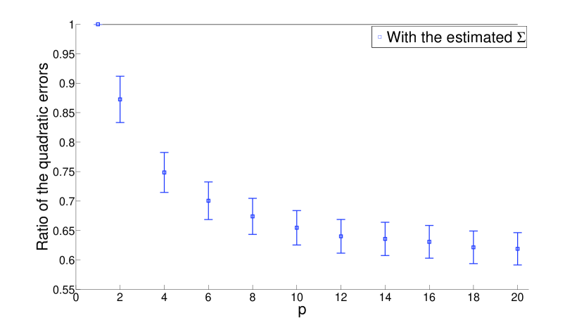
Figure 1: Increasing the number of tasks $p$ (Experiment A), improvement of multi-task compared to single-task: $\mathbb{E}[\lVert\widehat{f}_{\mathrm{similar},\widehat{\Sigma}}-f\rVert^{2}/\lVert\widehat{f}_{\mathrm{ind},\widehat{\Sigma}}-f\rVert^{2}]$.

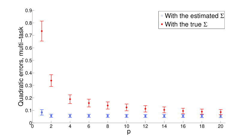
Figure 2: Increasing the number of tasks $p$ (Experiment A), quadratic errors of multi-task estimators $(np)^{-1}\mathbb{E}[\lVert\widehat{f}_{\mathrm{similar},S}-f\rVert^{2}]$. Blue: $S=\widehat{\Sigma}$. Red: $S=\Sigma$.

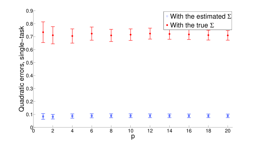
Figure 3: Increasing the number of tasks $p$ (Experiment A), quadratic errors of single-task estimators $(np)^{-1}\mathbb{E}[\lVert\widehat{f}_{\mathrm{ind},S}-f\rVert^{2}]$. Blue: $S=\widehat{\Sigma}$. Red: $S=\Sigma$.

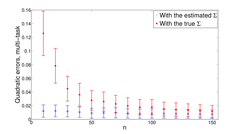
Figure 4: Increasing the sample size $n$ (Experiment B), quadratic errors of multi-task estimators $(np)^{-1}\mathbb{E}[\lVert\widehat{f}_{\mathrm{similar},S}-f\rVert^{2}]$. Blue: $S=\widehat{\Sigma}$. Red: $S=\Sigma$.

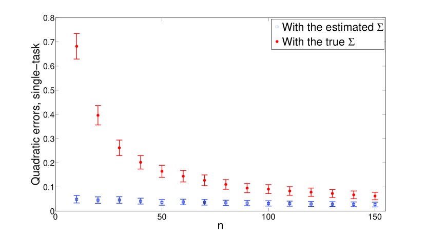
Figure 5: Increasing the sample size $n$ (Experiment B), quadratic errors of single-task estimators $(np)^{-1}\mathbb{E}[\lVert\widehat{f}_{\mathrm{ind},S}-f\rVert^{2}]$. Blue: $S=\widehat{\Sigma}$. Red: $S=\Sigma$.

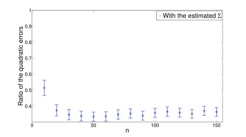
Figure 6: Increasing the sample size $n$ (Experiment B), improvement of multi-task compared to single-task: $\mathbb{E}[\lVert\widehat{f}_{\mathrm{similar},\widehat{\Sigma}}-f\rVert^{2}/\lVert\widehat{f}_{\mathrm{ind},\widehat{\Sigma}}-f\rVert^{2}]$.

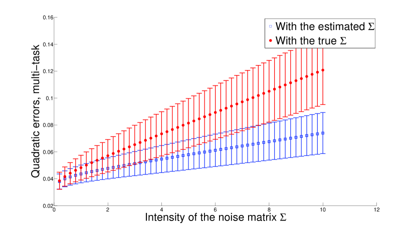
Figure 7: Increasing the signal-to-noise ratio (Experiment C), quadratic errors of multi-task estimators $(np)^{-1}\mathbb{E}[\lVert\widehat{f}_{\mathrm{similar},S}-f\rVert^{2}]$. Blue: $S=\widehat{\Sigma}$. Red: $S=\Sigma$.

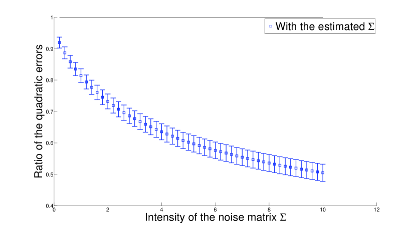
Figure 8: Increasing the signal-to-noise ratio (Experiment C), improvement of multi-task compared to single-task: $\mathbb{E}[\lVert\widehat{f}_{\mathrm{similar},\widehat{\Sigma}}-f\rVert^{2}/\lVert\widehat{f}_{\mathrm{ind},\widehat{\Sigma}}-f\rVert^{2}]$.

$t$	0.01	100
$\mathbb{E}[\lVert\widehat{f}_{\mathrm{similar},\widehat{\Sigma}}-f\rVert^{2}/\lVert\widehat{f}_{\mathrm{ind},\widehat{\Sigma}}-f\rVert^{2}]$	$1.80\pm 0.02$	$0.300\pm 0.003$
$\mathbb{E}[\lVert\widehat{f}_{\mathrm{similar},\widehat{\Sigma}}-f\rVert^{2}]$	$(2.27\pm 0.38)\times 10^{-2}$	$0.357\pm 0.048$
$\mathbb{E}[\lVert\widehat{f}_{\mathrm{similar},\Sigma}-f\rVert^{2}]$	$(1.20\pm 0.28)\times 10^{-2}$	$0.823\pm 0.080$
$\mathbb{E}[\lVert\widehat{f}_{\mathrm{ind},\widehat{\Sigma}}-f\rVert^{2}]$	$(1.26\pm 0.26)\times 10^{-2}$	$1.51\pm 0.07$
$\mathbb{E}[\lVert\widehat{f}_{\mathrm{ind},\Sigma}-f\rVert^{2}]$	$(1.20\pm 0.24)\times 10^{-2}$	$4.47\pm 0.13$

Table 1: Results of Experiment C for the extreme values of $t$.

$q$	$\mathbb{E}\left[q\right]$	$\textrm{Std}[q]$	p-value for $\mathbb{H}_{0}=\left\{q>1\right\}$
$\lVert\widehat{f}_{\mathrm{clus}}-f\rVert^{2}/\lVert\widehat{f}_{\mathrm{ind}}-f\rVert^{2}$	$0.668$	$0.294$	$<10^{-15}$
$\lVert\widehat{f}_{\mathrm{interval}}-f\rVert^{2}/\lVert\widehat{f}_{\mathrm{ind}}-f\rVert^{2}$	$0.660$	$0.270$	$<10^{-15}$
$\lVert\widehat{f}_{\mathrm{interval}}-f\rVert^{2}/\lVert\widehat{f}_{\mathrm{clus}}-f\rVert^{2}$	$1.00$	$0.165$	$0.50$

Table 2: Clustering and segmentation (Experiment D).

$q$	$n$	$\mathbb{E}\left[q\right]$	$\textrm{Std}[q]$	p-value for $\mathbb{H}_{0}=\left\{q>1\right\}$
$\lVert\widehat{f}_{\mathrm{similar},\widehat{\Sigma}_{\textrm{HM}}}-f\rVert^{2}/\lVert\widehat{f}_{\mathrm{similar},\textrm{CV}}-f\rVert^{2}$	10	$0.35$	$0.46$	$<10^{-15}$
$\lVert\widehat{f}_{\mathrm{similar},\widehat{\Sigma}_{\textrm{HM}}}-f\rVert^{2}/\lVert\widehat{f}_{\mathrm{similar},\textrm{CV}}-f\rVert^{2}$	50	$0.56$	$0.42$	$<10^{-15}$
$\lVert\widehat{f}_{\mathrm{similar},\widehat{\Sigma}_{\textrm{HM}}}-f\rVert^{2}/\lVert\widehat{f}_{\mathrm{similar},\textrm{CV}}-f\rVert^{2}$	100	$0.71$	$0.34$	$<10^{-15}$
$\lVert\widehat{f}_{\mathrm{similar},\widehat{\Sigma}_{\textrm{HM}}}-f\rVert^{2}/\lVert\widehat{f}_{\mathrm{similar},\textrm{CV}}-f\rVert^{2}$	250	$0.87$	$0.19$	$<10^{-15}$

Table 3: Comparison of our method to 5-fold cross-validation (Experiment E).

6.5 Comments

As expected, multi-task learning significantly helps when all $f^{j}$ are equal, as soon as $p$ is large enough (Figure 1), especially for small $n$ (Figure 6) and large noise-levels (Figure 8 and Table 1). Increasing the number of tasks rapidly reduces the quadratic error with multi-task estimators (Figure 2) contrary to what happens with single-task estimators (Figure 3).

A noticeable phenomenon also occurs in Figure 2 and even more in Figure 3: the estimator $\widehat{f}_{\mathrm{ind},\Sigma}$ (that is, obtained knowing the true covariance matrix $\Sigma$) is less efficient than $\widehat{f}_{\mathrm{ind},\widehat{\Sigma}}$ where the covariance matrix is estimated. It corresponds to the combination of two facts: (i) multiplying the ideal penalty by a small factor $1<C_{n}<1+o(1)$ is known to often improve performances in practice when the sample size is small (see Section 6.3.2 of Arlot, 2009), and (ii) minimal penalty algorithms like Algorithm 14 are conjectured to overpenalize slightly when $n$ is small or the noise-level is large (Lerasle, 2011) (as confirmed by Figure 7). Interestingly, this phenomenon is stronger for single-task estimators (differences are smaller in Figure 2) and disappears when $n$ is large enough (Figure 5), which is consistent with the heuristic motivating multi-task learning: “increasing the number of tasks $p$ amounts to increase the sample size”.

Figures 4 and 5 show that our procedure works well with small $n$, and that increasing $n$ does not seem to significantly improve the performance of our estimators, except in the single-task setting with $\Sigma$ known, where the over-penalization phenomenon discussed above disappears.

Table 2 shows that using the multitask procedure improves the estimation accuracy, both in the clustering setting and in the segmentation setting. The last line of Table 2 does not show that the clustering setting improves over the “segmentation into intervals” one, which was awaited if a model close to the oracle is selected in both cases.

Table 3 finally shows that our parameter tuning procedure outperforms 5-fold cross-validation.

7 Conclusion and Future Work

This paper shows that taking into account the unknown similarity between $p$ regression tasks can be done optimally (Theorem 26). The crucial point is to estimate the $p\times p$ covariance matrix $\Sigma$ of the noise (covariance between tasks), in order to learn the task similarity matrix $M$. Our main contributions are twofold. First, an estimator of $\Sigma$ is defined in Section 4, where non-asymptotic bounds on its error are provided under mild assumptions on the mean of the sample (Theorem 20). Second, we show an oracle inequality (Theorem 26), more particularly with a simplified estimation of $\Sigma$ and increased performances when the matrices of $\mathcal{M}$ are jointly diagonalizable (which often corresponds to cases where we have a prior knowledge of what the relations between the tasks would be). We do plan to expand our results to larger sets $\mathcal{M}$, which may require new concentration inequalities and new optimization algorithms.

Simulation experiments show that our algorithm works with reasonable sample sizes, and that our multi-task estimator often performs much better than its single-task counterpart. Up to the best of our knowledge, a theoretical proof of this point remains an open problem that we intend to investigate in a future work.

Acknowledgments

This paper was supported by grants from the Agence Nationale de la Recherche (Detect project, reference ANR-09-JCJC-0027-01) and from the European Research Council (SIERRA Project ERC-239993).

We give in Appendix the proofs of the different results stated in Sections 2, 4 and 5. The proofs of our main results are contained in Sections E and F.

A Proof of Proposition 8

Proof  It is sufficient to show that $\langle\cdot,\cdot\rangle_{\mathcal{G}}$ is positive-definite on $\mathcal{G}$. Take $g\in\mathcal{G}$ and $S=(S_{i,j})_{1\leq i\leq j\leq p}$ the symmetric postive-definite matrix of size $p$ verifying $S^{2}=M$, and denote $T=S^{-1}=(T_{i,j})_{1\leq i,j\leq p}$. Let $f$ be the element of $\mathcal{G}$ defined by $\forall i\in\{1\dots p\},\leavevmode\nobreak\ g(\cdot,i)=\sum_{k=1}^{n}T_{i,k}f(\cdot,k)$. We then have:

$$\langle g,g\rangle_{\mathcal{G}} =\sum_{i=1}^{p}\sum_{j=1}^{p}M_{i,j}\langle g(\cdot,i),g(\cdot,j)\rangle_{\mathcal{F}}$$

$$=\sum_{i=1}^{p}\sum_{j=1}^{p}\sum_{k=1}^{p}\sum_{l=1}^{p}M_{i,j}T_{i,k}T_{j,l}\langle f(\cdot,k),f(\cdot,l)\rangle_{\mathcal{F}}$$

$$=\sum_{j=1}^{p}\sum_{k=1}^{p}\sum_{l=1}^{p}T_{l,j}\langle f(\cdot,k),f(\cdot,l)\rangle_{\mathcal{F}}\sum_{i=1}^{p}M_{j,i}T_{i,k}$$

$$=\sum_{j=1}^{p}\sum_{k=1}^{p}\sum_{l=1}^{p}T_{l,j}\langle f(\cdot,k),f(\cdot,l)\rangle_{\mathcal{F}}(M\cdot T)_{j,k}$$

$$=\sum_{k=1}^{p}\sum_{l=1}^{p}T_{l,j}\langle f(\cdot,k),f(\cdot,l)\rangle_{\mathcal{F}}\sum_{j=1}^{p}T_{l,j}(M\cdot T)_{j,k}$$

$$=\sum_{k=1}^{p}\sum_{l=1}^{p}\langle f(\cdot,k),f(\cdot,l)\rangle_{\mathcal{F}}(T\cdot M\cdot T)_{k,l}$$

$$=\sum_{k=1}^{p}\|f(\cdot,k)\|_{\mathcal{F}}^{2}.$$

This shows that $\langle g,g\rangle_{\mathcal{G}}\geq 0$ and that $\langle g,g\rangle_{\mathcal{G}}=0\Rightarrow f=0\Rightarrow g=0$.  

B Proof of Corollary 9

Proof  If $(x,j)\in\mathcal{X}\times\{1,\dots,p\}$, the application $(f^{1},\dots,f^{p})\mapsto f^{j}(x)$ is clearly continuous. We now show that $(\mathcal{G},\langle\cdot,\cdot\rangle_{\mathcal{G}})$ is complete. If $(g_{n})_{n\in\mathbb{N}}$ is a Cauchy sequence of $\mathcal{G}$ and if we define, as in Section A, the functions $f_{n}$ by $\forall n\in\mathbb{N},\leavevmode\nobreak\ \forall i\in\{1\dots p\},\leavevmode\nobreak\ g_{n}(\cdot,i)=\sum_{k=1}^{p}T_{i,k}f_{n}(\cdot,k)$. The same computations show that $(f_{n}(\cdot,i))_{n\in\mathbb{N}}$ are Cauchy sequences of $\mathcal{F}$, and thus converge. So the sequence $(f_{n})_{n\in\mathbb{N}}$ converges in $\mathcal{G}$, and $(g_{n})_{n\in\mathbb{N}}$ does likewise.  

C Proof of Proposition 11

Proof  We define

$$\widetilde{\Phi}(x,j)=M^{-1}\cdot\begin{pmatrix}\delta_{1,j}\Phi(x)\\ \vdots\\ \delta_{p,j}\Phi(x)\\ \end{pmatrix}\enspace,$$

with $\delta_{i,j}=\mathbf{1}_{i=j}$ being the Kronecker symbol, that is, $\delta_{i,j}=1$ if $i=j$ and $0$ otherwise. We now show that $\widetilde{\Phi}$ is the feature function of the RKHS. For $g\in\mathcal{G}$ and $(x,l)\in\mathcal{X}\times\{1,\dots,p\}$, we have:

$$\langle g,\widetilde{\Phi}(x,l)\rangle_{\mathcal{G}} =\sum_{j=1}^{p}\sum_{i=1}^{p}M_{j,i}\langle g(\cdot,j),\widetilde{\Phi}(x,l)^{i}\rangle_{\mathcal{F}}$$

$$=\sum_{j=1}^{p}\sum_{i=1}^{p}\sum_{m=1}^{p}M_{j,i}M^{-1}_{i,m}\delta_{m,l}\langle g(\cdot,j),\Phi(x)\rangle_{\mathcal{F}}$$

$$=\sum_{j=1}^{p}\sum_{m=1}^{p}(M\cdot M^{-1})_{j,m}\delta_{m,l}g(x,j)$$

$$=\sum_{j=1}^{p}\delta_{j,l}g(x,j)=g(x,l)\enspace.$$

Thus we can write:

$$\widetilde{k}((x,i),(y,j)) =\langle\widetilde{\Phi}(x,i),\widetilde{\Phi}(y,j)\rangle_{\mathcal{G}}$$

$$=\sum_{h=1}^{p}\sum_{h^{\prime}=1}^{p}M_{h,h^{\prime}}\langle M^{-1}_{h,i}\Phi(x),M^{-1}_{h^{\prime},j}\Phi(y)\rangle_{\mathcal{F}}$$

$$=\sum_{h=1}^{p}\sum_{h^{\prime}=1}^{p}M_{h,h^{\prime}}M^{-1}_{h,i}M^{-1}_{h^{\prime},j}K(x,y)$$

$$=\sum_{h=1}^{p}M^{-1}_{h,i}(M\cdot M^{-1})_{h,j}K(x,y)$$

$$=\sum_{h=1}^{p}M^{-1}_{h,i}\delta_{h,j}K(x,y)=M^{-1}_{i,j}K(x,y)\enspace.$$

 

D Computation of the Quadratic Risk in Example 12

We consider here that $f^{1}=\dots=f^{p}$. We use the set $\mathcal{M}_{\mathrm{similar}}$:

$$\mathcal{M}_{\mathrm{similar}}:=\left\{M_{\mathrm{similar}}\left(\lambda,\mu\right)=(\lambda+p\mu)I_{p}-\frac{\mu}{p}\boldsymbol{1}\boldsymbol{1}^{\top}\,/\,(\lambda,\mu)\in(0,+\infty)^{2}\right\}$$

Using the estimator $\widehat{f}_{M}=A_{M}y$ we can then compute the quadratic risk using the bias-variance decomposition given in Equation (36):

$$\mathbb{E}\left[\left\|\widehat{f}_{M}-f\right\|_{2}^{2}\right]=\|(A_{M}-I_{np})f\|_{2}^{2}+\operatorname{tr}(A_{M}^{\top}A_{M}\cdot(\Sigma\otimes I_{n}))\enspace.$$

Les us denote by $(e_{1},\dots,e_{p})$ the canonical basis of $\mathbb{R}^{p}$. The eigenspaces of $p^{-1}\boldsymbol{1}\boldsymbol{1}^{\top}$ are:

• $\textrm{span}\left\{e_{1}+\dots+e_{p}\right\}$ corresponding to eigenvalue $p$,

• $\textrm{span}\left\{e_{2}-e_{1},\dots,e_{p}-e_{1}\right\}$ corresponding to eigenvalue $0$.

Thus, with $\widetilde{\mu}=\lambda+p\mu$ we can diagonalize in an orthonormal basis any matrix $M_{\lambda,\mu}\in\mathcal{M}$ as $M=P^{\top}D_{\lambda,\widetilde{\mu}}P$, with $D=D_{\lambda,\widetilde{\mu}}=\operatorname{Diag}\{\lambda,\widetilde{\mu},\dots,\widetilde{\mu}\}$. Les us also diagonalise in an orthonormal basis $K$: $K=Q^{\top}\Delta Q$, $\Delta=\operatorname{Diag}\{\mu_{1},\dots,\mu_{n}\}$. Thus we can write (see Properties 38 and 39 for basic properties of the Kronecker product):

$$A_{M}=A_{M_{\lambda,\mu}}=(P^{\top}\otimes Q^{\top})\left[(D^{-1}\otimes\Delta)\left((D^{-1}\otimes\Delta)+npI_{np}\right)^{-1}\right](P\otimes Q)\enspace.$$

We can then note that $(D^{-1}\otimes\Delta)\left((D^{-1}\otimes\Delta)+npI_{np}\right)^{-1}$ is a diagonal matrix, whose diagonal entry of index $(j-1)n+i$ ($i\in\{1,\dots,n\}$, $j\in\{1,\dots,p\}$) is

$$\left\{\begin{array}[]{lr}&\frac{\mu_{i}}{\mu_{i}+np\lambda}\textrm{ if }j=1\enspace,\\ &\frac{\mu_{i}}{\mu_{i}+np\widetilde{\mu}}\textrm{ if }j>1\enspace.\end{array}\right.$$

We can now compute both bias and variance.

Bias:

We can first remark that $(P^{\top}\otimes Q^{\top})=(P\otimes Q)^{\top}$ is an orthogonal matrix and that $P\times\boldsymbol{1}=(1,0,\dots,0)^{\top}$. Thus, as in this setting $f^{1}=\dots=f^{p}$, we have $f=\boldsymbol{1}\otimes(f^{1}(X_{1}),\dots,f^{1}(X_{n}))^{\top}$ and $(P^{\top}\otimes Q^{\top})f=(1,0,\dots,0)^{\top}\otimes Q(f^{1}(X_{1}),\dots,f^{1}(X_{n}))^{\top}$. To keep notations simple we note $Q(f^{1}(X_{1}),\dots,f^{1}(X_{n}))^{\top}:=(g_{1},\dots,g_{n})^{\top}$. Thus

$$\|(A_{M}-I_{np})f\|_{2}^{2} =\|(P\otimes Q)^{\top}\left[(D^{-1}\otimes K)\left((D^{-1}\otimes K)+npI_{np}\right)^{-1}-I_{np}\right](P\otimes Q)f\|_{2}^{2}$$

$$=\|\left[(D^{-1}\otimes\Delta)\left((D^{-1}\otimes\Delta)+npI_{np}\right)^{-1}-I_{np}\right]$$

$$\leavevmode\nobreak\ \leavevmode\nobreak\ \leavevmode\nobreak\ \leavevmode\nobreak\ \leavevmode\nobreak\ \leavevmode\nobreak\ \leavevmode\nobreak\ \leavevmode\nobreak\ \leavevmode\nobreak\ \leavevmode\nobreak\ \leavevmode\nobreak\ \leavevmode\nobreak\ \leavevmode\nobreak\ \leavevmode\nobreak\ \times(1,0,\dots,0)^{\top}\otimes(g_{1},\dots,g_{n})^{\top}\|_{2}^{2}\enspace.$$

As only the first $n$ terms of $(P\otimes Q)f$ are non-zero we can finally write

$$\|(A_{M}-I_{np})f\|_{2}^{2}=\sum_{i=1}^{n}\left(\frac{np\lambda}{\mu_{i}+np\lambda}\right)^{2}g_{i}^{2}\enspace.$$

Variance:

First note that

$$(P\otimes Q)(\Sigma\otimes I_{n})(P\otimes Q)^{\top}=(P\Sigma P^{\top}\otimes I_{n})\enspace.$$

We can also note that $\widetilde{\Sigma}:=P\Sigma P^{\top}$ is a symmetric positive definite matrix, with positive diagonal coefficients. Thus we can finally write

$$\operatorname{tr}(A_{M}^{\top}A_{M}\cdot(\Sigma\otimes I_{n})) =\operatorname{tr}\bigg{(}P\otimes Q)^{\top}\left[(D^{-1}\otimes\Delta)\left((D^{-1}\otimes\Delta)+npI_{np}\right)^{-1}\right]^{2}$$

$$\leavevmode\nobreak\ \leavevmode\nobreak\ \leavevmode\nobreak\ \leavevmode\nobreak\ \leavevmode\nobreak\ \leavevmode\nobreak\ \leavevmode\nobreak\ \leavevmode\nobreak\ \leavevmode\nobreak\ \leavevmode\nobreak\ \leavevmode\nobreak\ \leavevmode\nobreak\ \leavevmode\nobreak\ \leavevmode\nobreak\ \times(P\otimes Q)(\Sigma\otimes I_{n})\bigg{)}$$

$$=\operatorname{tr}\bigg{(}\left[(D^{-1}\otimes\Delta)\left((D^{-1}\otimes\Delta)+npI_{np}\right)^{-1}\right]^{2}$$

$$\leavevmode\nobreak\ \leavevmode\nobreak\ \leavevmode\nobreak\ \leavevmode\nobreak\ \leavevmode\nobreak\ \leavevmode\nobreak\ \leavevmode\nobreak\ \leavevmode\nobreak\ \leavevmode\nobreak\ \leavevmode\nobreak\ \leavevmode\nobreak\ \leavevmode\nobreak\ \leavevmode\nobreak\ \leavevmode\nobreak\ \times(P\otimes Q)(\Sigma\otimes I_{n})(P\otimes Q)^{\top}\bigg{)}$$

$$=\sum_{i=1}^{n}\left[\left(\frac{\mu_{i}}{\mu_{i}+np\lambda}\right)^{2}\widetilde{\Sigma}_{1,1}+\left(\frac{\mu_{i}}{\mu_{i}+np\widetilde{\mu}}\right)^{2}\sum_{j=2}^{p}\widetilde{\Sigma}_{j,j}\right]\enspace.$$

As noted at the end of Example 12 this leads to an oracle which has all its $p$ functions equal.

D.1 Proof of Equation (19) in Section 5.2

Let $M\in\mathcal{S}_{p}^{++}(\mathbb{R})$, $P\in\mathcal{O}_{p}(\mathbb{R})$ such that $M=P^{\top}\operatorname{Diag}(d_{1},\dots,d_{p})P$ and $\widetilde{\Sigma}=P\Sigma P^{\top}$. We recall that $A_{\lambda}=K(K+n\lambda I_{n})^{-1}$. The computations detailed above also show that the ideal penalty introduced in Equation (7) can be written as

$$\operatorname{pen}_{\operatorname{id}}(M)=\frac{2\operatorname{tr}\big{(}A_{M}\cdot(\Sigma\otimes I_{n})\big{)}}{np}=\frac{2}{np}\left(\sum_{j=1}^{p}\operatorname{tr}(A_{pd_{j}})\widetilde{\Sigma}_{j,j}\right)\enspace.$$

E Proof of Theorem 20

Theorem 20 is proved in this section, after stating some classical linear algebra results (Section E.1).

E.1 Some Useful Tools

We now give two properties of the Kronecker product, and then introduce a useful norm on $\mathcal{S}_{p}(\mathbb{R})$, upon which we give several properties. Those are the tools needed to prove Theorem 20.

Property 38

The Kronecker product is bilinear, associative and for every matrices $A,B,C,D$ such that the dimensions fit, $(A\otimes B)(C\otimes D)=(AC)\otimes(BD)$.

Property 39

Let $A\in\mathcal{M}_{n}(\mathbb{R})$, $B\in\mathcal{M}_{B}(\mathbb{R})$, $(A\otimes B)^{\top}=(A^{\top}\otimes B^{\top})$.

Definition 40

We now introduce the norm $|\!|\!|\cdot|\!|\!|$ on $\mathcal{S}_{p}(\mathbb{R})$, which is the modulus of the eigenvalue of largest magnitude, and can be defined by

$$|\!|\!|S|\!|\!|:=\sup_{z\in\mathbb{R}^{p},\left\|z\right\|_{2}=1}\left\lvert z^{\top}Sz\right\rvert\enspace.$$

This norm has several interesting properties, some of which we will use are stated below.

Property 41

The norm $|\!|\!|\cdot|\!|\!|$ is a matricial norm: $\forall(A,B)\in\mathcal{S}_{p}(\mathbb{R})^{2},\leavevmode\nobreak\ |\!|\!|AB|\!|\!|\leq|\!|\!|A|\!|\!||\!|\!|B|\!|\!|$.

We will use the following result, which is a consequence of the preceding Property.

$$\forall S\in\mathcal{S}_{p}(\mathbb{R}),\leavevmode\nobreak\ \forall T\in\mathcal{S}_{p}^{++}(\mathbb{R}),\leavevmode\nobreak\ |\!|\!|T^{-\frac{1}{2}}ST^{-\frac{1}{2}}|\!|\!|\leq|\!|\!|S|\!|\!||\!|\!|T^{-1}|\!|\!|\enspace.\\$$

We also have:

Proposition 42

$$\forall\Sigma\in\mathcal{S}_{p}(\mathbb{R}),\leavevmode\nobreak\ |\!|\!|\Sigma\otimes I_{n}|\!|\!|=|\!|\!|\Sigma|\!|\!|\enspace.$$

Proof  We can diagonalize $\Sigma$ in an orthonormal basis: $\exists U\in\mathcal{O}_{n}(\mathbb{R}),\leavevmode\nobreak\ \exists D=\textrm{Diag}(\mu_{1},\dots,\mu_{p}),\leavevmode\nobreak\ \Sigma=U^{\top}DU$. We then have, using the properties of the Kronecker product:

$$\Sigma\otimes I_{n} =(U^{\top}\otimes I_{n})(D\otimes I_{n})(U\otimes I_{n})$$

$$=(U\otimes I_{n})^{\top}(D\otimes I_{n})(U\otimes I_{n})\enspace.$$

We just have to notice that $U\otimes I_{n}\in\mathcal{O}_{np}(\mathbb{R})$ and that:

$$D\otimes I_{n}=\textrm{Diag}(\underbrace{\mu_{1},\dots,\mu_{1}}_{n\textrm{ times}},\dots,\underbrace{\mu_{p},\dots,\mu_{p}}_{n\textrm{ times}})\enspace.$$

 
This norm can also be written in other forms:

Property 43

If $M\in\mathcal{M}_{n}(\mathbb{R})$, the operator norm $\left\lVert M\right\rVert_{2}:=\sup_{t\in\mathbb{R}^{n}\backslash\{0\}}\left\{\frac{\|Mt\|_{2}}{\|t\|_{2}}\right\}$ is equal to the greatest singular value of $M$: $\sqrt{\rho(M^{\top}M)}$. Henceforth, if $S$ is symmetric, we have $|\!|\!|S|\!|\!|=\|S\|_{2}$

E.2 The Proof

We now give a proof of Theorem 20, using Lemmas 46, 48 and 49, which are stated and proved in Section E.3. The outline of the proof is the following:

1. Apply Theorem 15 to problem (10) for every $z\in\mathcal{Z}$ in order to

2. control $\left\lVert s-\zeta\right\rVert_{\infty}$ with a large probability, where $s,\zeta\in\mathbb{R}^{p(p+1)/2}$ are defined by

   $$s :=(\Sigma_{1,1},\ldots,\Sigma_{p,p},\Sigma_{1,1}+\Sigma_{2,2}+2\Sigma_{1,2},\ldots,\Sigma_{i,i}+\Sigma_{j,j}+2\Sigma_{i,j},\ldots)$$

   $$\mbox{and}\quad\zeta :=(a(e_{1}),\ldots,a(e_{p}),a(e_{1}+e_{2}),\ldots,a(e_{1}+e_{p}),a(e_{2}+e_{3}),\ldots,a(e_{p-1}+e_{p}))\enspace.$$

3. Deduce that $\widehat{\Sigma}=J(\zeta)$ is close to $\Sigma=J(s)$ by controlling the Lipschitz norm of $J$.

Proof  1. Apply Theorem 15: We start by noticing that Assumption (13) actually holds true with all $\lambda_{0,j}$ equal. Indeed, let $(\lambda_{0,j})_{1\leq j\leq p}$ be given by Assumption (13) and define $\lambda_{0}:=\min_{j=1,\ldots,p}\lambda_{0,j}$. Then, $\lambda_{0}\in(0,+\infty)$ and $\operatorname{df}(\lambda_{0})$ since all $\lambda_{0,j}$ satisfy these two conditions. For the last condition, remark that for every $j\in\{1,\ldots,p\}$, $\lambda_{0}\leq\lambda_{0,j}$ and $\lambda\mapsto\lVert(A_{\lambda}-I)F_{e_{j}}\rVert_{2}^{2}$ is a nonincreasing function (as noticed in Arlot and Bach, 2011 for instance), so that

$$\frac{1}{n}\left\lVert(A_{\lambda_{0}}-I_{n})F_{e_{j}}\right\rVert_{2}^{2}\leq\frac{1}{n}\left\lVert(A_{\lambda_{0,j}}-I_{n})F_{e_{j}}\right\rVert_{2}^{2}\leq\Sigma_{j,j}\sqrt{\frac{\ln(n)}{n}}\enspace.$$ (23)

In particular, Equation (8) holds with $d_{n}=1$ for problem (10) whatever $z\in\{e_{1},\ldots,e_{p}\}$.

Let us now consider the case $z=e_{i}+e_{j}$ with $i\neq j\in\{1,\ldots,p\}$. Using Equation (23) and that $F_{e_{i}+e_{j}}=F_{e_{i}}+F_{e_{j}}$, we have

$$\left\lVert(B_{\lambda_{0}}-I_{n})F_{e_{i}+e_{j}}\right\rVert_{2}^{2}\leq\left\lVert(B_{\lambda_{0}}-I_{n})F_{e_{i}}\right\rVert_{2}^{2}+\left\lVert(B_{\lambda_{0}}-I_{n})F_{e_{j}}\right\rVert_{2}^{2}+2\langle(B_{\lambda_{0}}-I_{n})F_{e_{i}},(B_{\lambda_{0}}-I_{n})F_{e_{j}}\rangle\enspace.$$

The last term is bounded as follows:

$$2\langle(B_{\lambda_{0}}-I_{n})F_{e_{i}},(B_{\lambda_{0}}-I_{n})F_{e_{j}}\rangle \leq 2\|(B_{\lambda_{0}}-I_{n})F_{e_{i}}\|\cdot\|(B_{\lambda_{0}}-I_{n})F_{e_{j}}\|$$

$$\leq 2\sqrt{n\ln(n)}\sqrt{\Sigma_{i,i}\Sigma_{j,j}}$$

$$\leq\sqrt{n\ln(n)}(\Sigma_{i,i}+\Sigma_{j,j})$$

$$\leq(1+c(\Sigma))\sqrt{n\ln(n)}(\Sigma_{i,i}+\Sigma_{j,j}+2\Sigma_{i,j})$$

$$=(1+c(\Sigma))\sqrt{n\ln(n)}\sigma^{2}_{e_{i}+e_{j}}\enspace,$$

because Lemma 46 shows

$$2(\Sigma_{i,i}+\Sigma_{j,j})\leq(1+c(\Sigma))(\Sigma_{i,i}+\Sigma_{j,j}+2\Sigma_{i,j})\enspace.$$

Therefore, Equation (8) holds with $d_{n}=1+c(\Sigma)$ for problem (10) whatever $z\in\mathcal{Z}$.

2. Control $\left\lVert s-\zeta\right\rVert_{\infty}$: Let us define

$$\eta_{1}:=\beta(2+\delta)(1+c(\Sigma))\sqrt{\frac{\ln(n)}{n}}\enspace.$$

By Theorem 15, for every $z\in\mathcal{Z}$, an event $\Omega_{z}$ of probability greater than $1-n^{-\delta}$ exists on which, if $n\geq n_{0}(\delta)$,

$$(1-\eta_{1})\sigma_{z}^{2}\leq a(z)\leq(1+\eta_{1})\sigma_{z}^{2}\enspace.$$

So, on $\Omega:=\bigcap_{z\in Z}\Omega_{z}$,

$$\left\lVert\zeta-s\right\rVert_{\infty}\leq\eta_{1}\left\lVert s\right\rVert_{\infty}\enspace,$$ (24)

and $\mathbb{P}(\Omega)\geq 1-p(p+1)/2\times n^{-\delta}$ by the union bound. Let

$$\left\lVert\Sigma\right\rVert_{\infty}:=\sup_{i,j}\left\lvert\Sigma_{i,j}\right\rvert\quad\mbox{and}\quad C_{1}(p):=\sup_{\Sigma\in\mathcal{S}_{p}(\mathbb{R})}\left\{\frac{\left\lVert\Sigma\right\rVert_{\infty}}{|\!|\!|\Sigma|\!|\!|}\right\}\enspace.$$

Since $\left\lVert s\right\rVert_{\infty}\leq 4\left\lVert\Sigma\right\rVert_{\infty}$ and $C_{1}(p)=1$ by Lemma 48, Equation (24) implies that on $\Omega$,

$$\left\lVert\zeta-s\right\rVert_{\infty}\leq 4\eta_{1}\left\lVert\Sigma\right\rVert_{\infty}\leq 4\eta_{1}|\!|\!|\Sigma|\!|\!|\enspace.$$ (25)

3. Conclusion of the proof: Let

$$C_{2}(p):=\sup_{\zeta\in\mathbb{R}^{p(p+1)/2}}\left\{\frac{|\!|\!|J(\zeta)|\!|\!|}{\left\lVert\zeta\right\rVert_{\infty}}\right\}\enspace.$$

By Lemma 49, $C_{2}(p)\leq\frac{3}{2}p$. By Equation (25), on $\Omega$,

$$|\!|\!|\widehat{\Sigma}-\Sigma|\!|\!|=|\!|\!|J(\zeta)-J(s)|\!|\!|\leq C_{2}(p)\left\lVert\zeta-s\right\rVert_{\infty}\leq 4\eta_{1}C_{2}(p)|\!|\!|\Sigma|\!|\!|\enspace.$$ (26)

Since

$$|\!|\!|\Sigma^{-\frac{1}{2}}\widehat{\Sigma}\Sigma^{-\frac{1}{2}}-I_{p}|\!|\!|=|\!|\!|\Sigma^{-\frac{1}{2}}(\Sigma-\widehat{\Sigma})\Sigma^{-\frac{1}{2}}|\!|\!|\leq|\!|\!|\Sigma^{-1}|\!|\!||\!|\!|\Sigma-\widehat{\Sigma}|\!|\!|\enspace,$$

and $|\!|\!|\Sigma|\!|\!||\!|\!|\Sigma^{-1}|\!|\!|=c(\Sigma)$, Equation (26) implies that on $\Omega$,

$$|\!|\!|\Sigma^{-\frac{1}{2}}\widehat{\Sigma}\Sigma^{-\frac{1}{2}}-I_{p}|\!|\!|\leq 4\eta_{1}C_{2}(p)|\!|\!|\Sigma|\!|\!||\!|\!|\Sigma^{-1}|\!|\!|=4\eta_{1}C_{2}(p)c(\Sigma)\leq 6\eta_{1}pc(\Sigma)\enspace.$$

To conclude, Equation (14) holds on $\Omega$ with

$$\eta=6pc(\Sigma)\beta(2+\delta)(1+c(\Sigma))\sqrt{\frac{\ln(n)}{n}}\leq L_{1}(2+\delta)p\sqrt{\frac{\ln(n)}{n}}c(\Sigma)^{2}$$ (27)

for some numerical constant $L_{1}$.  

Remark 44

As stated in Arlot and Bach (2011), we need $\sqrt{n_{0}(\delta)/\ln(n_{0}(\delta))}\geq 504$ and $\sqrt{n_{0}(\delta)}/\ln(n_{0}(\delta))\geq 24(290+\delta)$.

Remark 45

To ensure that the estimated matrix $\widehat{\Sigma}$ is positive-definite we need that $\eta<1$, that is,

$$\sqrt{\frac{n}{\ln(n)}}>6\beta(2+\delta)pc(\Sigma)\left(1+c(\Sigma)\right)\enspace.$$

E.3 Useful Lemmas

Lemma 46

Let $p\geq 1$, $\Sigma\in\mathcal{S}_{p}^{++}(\mathbb{R})$ and $c(\Sigma)$ its condition number. Then,

$$\forall 1\leq i<j\leq p\,,\quad\Sigma_{i,j}\geq-\frac{c(\Sigma)-1}{c(\Sigma)+1}\frac{\Sigma_{i,i}+\Sigma_{j,j}}{2}\enspace,$$ (28)

Remark 47

The proof of Lemma 46 shows the constant $\frac{c(\Sigma)-1}{c(\Sigma)+1}$ cannot be improved without additional assumptions on $\Sigma$.

Proof  It suffices to show the result when $p=2$. Indeed, (28) only involves $2\times 2$ submatrices $\widetilde{\Sigma}(i,j)\in\mathcal{S}_{2}^{++}(\mathbb{R})$ for which

$$1\leq c(\widetilde{\Sigma})\leq c\left(\Sigma\right)\quad\mbox{hence}\quad 0\leq\frac{c(\widetilde{\Sigma})-1}{c(\widetilde{\Sigma})+1}\leq\frac{c(\Sigma)-1}{c(\Sigma)+1}\enspace.$$

So, some $\theta\in\mathbb{R}$ exists such that $\Sigma=|\!|\!|\Sigma|\!|\!|R_{\theta}^{\top}DR_{\theta}$ where

$$R_{\theta}:=\begin{pmatrix}\cos(\theta)&\sin(\theta)\\ -\sin(\theta)&\cos(\theta)\end{pmatrix}\qquad D=\begin{pmatrix}1&0\\ 0&\lambda\end{pmatrix}\quad\mbox{and}\quad\lambda:=\frac{1}{c(\Sigma)}\enspace.$$

Therefore,

$$\Sigma=|\!|\!|\Sigma|\!|\!|\begin{pmatrix}\cos^{2}(\theta)+\lambda\sin^{2}(\theta)&\frac{1-\lambda}{2}\sin(2\theta)\\ \frac{1-\lambda}{2}\sin(2\theta)&\lambda\cos^{2}(\theta)+\sin^{2}(\theta)\end{pmatrix}\enspace.$$

So, Equation (28) is equivalent to

$$\frac{(1-\lambda)\sin(2\theta)}{2}\geq-\frac{1-\lambda}{1+\lambda}\frac{1+\lambda}{2}\enspace,$$

which holds true for every $\theta\in\mathbb{R}$, with equality for $\theta\equiv\pi/2$ (mod. $\pi$).  

Lemma 48

For every $p\geq 1$, $C_{1}(p):=\sup_{\Sigma\in\mathcal{S}_{p}(\mathbb{R})}\frac{\|\Sigma\|_{\infty}}{|\!|\!|\Sigma|\!|\!|}=1\enspace.$

Proof  With $\Sigma=I_{p}$ we have $\|\Sigma\|_{\infty}=|\!|\!|\Sigma|\!|\!|=1$, so $C_{1}(p)\geq 1$.
Let us introduce $(i,j)$ such that $|\Sigma_{i,j}|=\|\Sigma\|_{\infty}$. We then have, with $e_{k}$ being the $k^{\textrm{th}}$ vector of the canonical basis of $\mathbb{R}^{p}$,

$$|\Sigma_{i,j}|=|e_{i}^{\top}\Sigma e_{j}|\leq|e_{i}^{\top}\Sigma e_{i}|^{1/2}|e_{j}^{\top}\Sigma e_{j}|^{1/2}\leq(\left\|\Sigma\right\|_{2}^{1/2})^{2}\enspace.$$

 

Lemma 49

For every $p\geq 1$, let $C_{2}(p):=\sup_{\zeta\in\mathbb{R}^{p(p+1)/2}}\frac{|\!|\!|J(\zeta)|\!|\!|}{\|\zeta\|_{\infty}}$. Then,

$$\frac{p}{4}\leq C_{2}(p)\leq\frac{3}{2}p\enspace.$$

Proof  For the lower bound, we consider

$$\zeta_{1}=(\underbrace{1,\dots,1}_{p\textrm{ times}},\underbrace{4,\dots,4}_{\frac{p(p-1)}{2}\textrm{ times}})\,,\quad\mbox{then}\quad J(\zeta_{1})=\begin{pmatrix}1&\ldots&1\\ \vdots&\ddots&\vdots\\ 1&\ldots&1\end{pmatrix}$$

so that $|\!|\!|J(\zeta)|\!|\!|=p$ and $\|\zeta\|_{\infty}=4$.

For the upper bound, we have for every $\zeta\in\mathbb{R}^{p(p+1)/2}$ and $z\in\mathbb{R}^{p}$ such that $\left\|z\right\|_{2}=1$

$$z^{\top}J(\zeta)z=\left\lvert\sum_{1\leq i,j\leq p}z_{i}z_{j}J(\zeta)_{i,j}\right\rvert\leq\sum_{1\leq i,j\leq p}\left\lvert z_{i}\right\rvert\left\lvert z_{j}\right\rvert\left\lvert J(\zeta)\right\rvert\leq\left\lVert J(\zeta)\right\rVert_{\infty}\left\lVert z\right\rVert_{1}^{2}\enspace.$$

By definition of $J$, $\lVert J(\zeta)\rVert_{\infty}\leq 3/2\left\lVert\zeta\right\rVert_{\infty}$. Remarking that $\lVert z\rVert_{1}^{2}\leq p\left\lVert z\right\rVert_{2}^{2}$ yields the result.  

F Proof of Theorem 26

The proof of Theorem 26 is similar to the proof of Theorem 3 in Arlot and Bach (2011). We give it here for the sake of completeness. We also show how to adapt its proof to demonstrate Theorem 29. The two main mathematical results used here are Theorem 20 and a gaussian concentration inequality from Arlot and Bach (2011).

F.1 Key Quantities and their Concentration Around their Means

Definition 50

We introduce, for $S\in\mathcal{S}_{p}^{++}(\mathbb{R})$,

$$\widehat{M}_{o}(S)\in\underset{M\in\mathcal{M}}{\operatorname{argmin}}\left\{\left\|\widehat{F}_{M}-Y\right\|_{2}+2\operatorname{tr}\left(A_{M}\cdot(S\otimes I_{n})\right)\right\}$$ (29)

Definition 51

Let $S\in\mathcal{S}_{p}(\mathbb{R})$, we note $S_{+}$ the symmetric matrix where the eigenvalues of $S$ have been thresholded at $0$. That is, if $S=U^{\top}DU$, with $U\in\mathcal{O}_{p}(\mathbb{R})$ and $D=\operatorname{Diag}(d_{1},\dots,d_{p})$, then

$$S_{+}:=U^{\top}\operatorname{Diag}\left(\max\left\{d_{1},0\right\},\dots,\max\left\{d_{n},0\right\}\right)U\enspace.$$

Definition 52

For every $M\in\mathcal{M}$, we define

$$b(M) =\|(A_{M}-I_{np})f\|_{2}^{2}\enspace,$$

$$v_{1}(M) =\mathbb{E}\left[\langle\varepsilon,A_{M}\varepsilon\rangle\right]=\operatorname{tr}(A_{M}\cdot(\Sigma\otimes I_{n}))\enspace,$$

$$\delta_{1}(M) =\langle\varepsilon,A_{M}\varepsilon\rangle-\mathbb{E}\left[\langle\varepsilon,A_{M}\varepsilon\rangle\right]=\langle\varepsilon,A_{M}\varepsilon\rangle-\operatorname{tr}(A_{M}\cdot(\Sigma\otimes I_{n}))\enspace,$$

$$v_{2}(M) =\mathbb{E}\left[\|A_{M}\varepsilon\|_{2}^{2}\right]=\operatorname{tr}(A_{M}^{\top}A_{M}\cdot(\Sigma\otimes I_{n}))\enspace,$$

$$\delta_{2}(M) =\|A_{M}\varepsilon\|_{2}^{2}-\mathbb{E}\left[\|A_{M}\varepsilon\|_{2}^{2}\right]=\|A_{M}\varepsilon\|_{2}^{2}-\operatorname{tr}(A_{M}^{\top}A_{M}\cdot(\Sigma\otimes I_{n}))\enspace,$$

$$\delta_{3}(M) =2\langle A_{M}\varepsilon,(A_{M}-I_{np})f\rangle\enspace,$$

$$\delta_{4}(M) =2\langle\varepsilon,(I_{np}-A_{M})f\rangle\enspace,$$

$$\widehat{\Delta}(M) =-2\delta_{1}(M)+\delta_{4}(M)\enspace.$$

Definition 53

Let $C_{A},C_{B},C_{C},C_{D},C_{E},C_{F}$ be fixed nonnegative constants. For every $x\geq 0$ we define the event

$$\Omega_{x}=\Omega_{x}(\mathcal{M},C_{A},C_{B},C_{C},C_{D},C_{E},C_{F})$$

on which, for every $M\in\mathcal{M}$ and $\theta_{1},\theta_{2},\theta_{3},\theta_{4}\in(0,1]$:

$$|\delta_{1}(M)| \leq\theta_{1}\operatorname{tr}\left(A_{M}^{\top}A_{M}\cdot(\Sigma\otimes I_{n})\right)+(C_{A}+C_{B}\theta_{1}^{-1})x|\!|\!|\Sigma|\!|\!|$$ (30)

$$|\delta_{2}(M)| \leq\theta_{2}\operatorname{tr}\left(A_{M}^{\top}A_{M}\cdot(\Sigma\otimes I_{n})\right)+(C_{C}+C_{D}\theta_{2}^{-1})x|\!|\!|\Sigma|\!|\!|$$ (31)

$$|\delta_{3}(M)| \leq\theta_{3}\left\|(I_{np}-A_{M})f\right\|_{2}^{2}+C_{E}\theta_{3}^{-1}x|\!|\!|\Sigma|\!|\!|$$ (32)

$$|\delta_{4}(M)| \leq\theta_{4}\left\|(I_{np}-A_{M})f\right\|_{2}^{2}+C_{F}\theta_{4}^{-1}x|\!|\!|\Sigma|\!|\!|$$ (33)

Of key interest is the concentration of the empirical processes $\delta_{i}$, uniformly over $M\in\mathcal{M}$. The following Lemma introduces such a result, when $\mathcal{M}$ contains symmetric matrices parametrized with their eigenvalues (with fixed eigenvectors).

Lemma 54

Let

$$C_{A}=2,\leavevmode\nobreak\ C_{B}=1,\leavevmode\nobreak\ C_{C}=2,\leavevmode\nobreak\ C_{D}=1,\leavevmode\nobreak\ C_{E}=306.25,\leavevmode\nobreak\ C_{F}=306.25\enspace.$$

Suppose that (18) holds. Then $\mathbb{P}(\Omega_{x}(\mathcal{M},C_{A},C_{B},C_{C},C_{D},C_{E},C_{F}))\geq 1-pe^{1027+\ln(n)}e^{-x}$. Suppose that (15) holds. Then $\mathbb{P}(\Omega_{x}(\mathcal{M},C_{A},C_{B},C_{C},C_{D},C_{E},C_{F}))\geq 1-6p\operatorname{card}(\mathcal{M})e^{-x}$.

$$\enspace.$$

Proof 

First common step.

Let $M\in\mathcal{M}$, $P_{M}\in\mathcal{O}_{p}(\mathbb{R})$ such that $M=P_{M}^{\top}DP_{M}$, with $D=\operatorname{Diag}(d_{1},\dots,d_{p})$. We can write:

$$A_{M}=A_{d_{1},\dots,d_{p}} =(P_{M}\otimes I_{n})^{\top}\left[(D^{-1}\otimes K)\left(D^{-1}\otimes K+npI_{np}\right)^{-1}\right](P_{M}\otimes I_{n})$$

$$=Q^{\top}\widetilde{A}_{d_{1},\dots,d_{p}}Q\enspace,$$

with $Q=P_{M}\otimes I_{n}$ and $\widetilde{A}_{d_{1},\dots,d_{p}}=(D^{-1}\otimes K)(D^{-1}\otimes K+npI_{np})^{-1}$. Remark that $\widetilde{A}_{d_{1},\dots,d_{p}}$ is block-diagonal, with diagonal blocks being $B_{d_{1}},\dots,B_{d_{p}}$ using the notations of Section 3. With $\widetilde{\varepsilon}=Q\varepsilon=(\widetilde{\varepsilon_{1}}^{\top},\dots,\widetilde{\varepsilon_{p}}^{\top})^{\top}$ and $\widetilde{f}=Qf=(\widetilde{f_{1}}^{\top},\dots,\widetilde{f_{p}}^{\top})^{\top}$ we can write

$$|\delta_{1}(M)| =\langle\widetilde{\varepsilon},\widetilde{A}_{d_{1},\dots,d_{p}}\widetilde{\varepsilon}\rangle-\mathbb{E}\left[\langle\widetilde{\varepsilon},\widetilde{A}_{d_{1},\dots,d_{p}}\widetilde{\varepsilon}\rangle\right]\enspace,$$

$$|\delta_{2}(M)| =\left\|\widetilde{A}_{d_{1},\dots,d_{p}}\widetilde{\varepsilon}\right\|_{2}^{2}-\mathbb{E}\left[\left\|\widetilde{A}_{d_{1},\dots,d_{p}}\widetilde{\varepsilon}\right\|_{2}^{2}\right]\enspace,$$

$$|\delta_{3}(M)| =2\langle\widetilde{A}_{d_{1},\dots,d_{p}}\widetilde{\varepsilon},(\widetilde{A}_{d_{1},\dots,d_{p}}-I_{np})\widetilde{f}\rangle\enspace,$$

$$|\delta_{4}(M)| =2\langle\widetilde{\varepsilon},(I_{np}-\widetilde{A}_{d_{1},\dots,d_{p}})\widetilde{f}\rangle\enspace.$$

We can see that the quantities $\delta_{i}$ decouple, therefore

$$|\delta_{1}(M)| =\sum_{i=1}^{p}\langle\widetilde{\varepsilon}_{i},A_{pd_{i}}\widetilde{\varepsilon}_{i}\rangle-\mathbb{E}\left[\langle\widetilde{\varepsilon}_{i},A_{pd_{i}}\widetilde{\varepsilon}\rangle\right]\enspace,$$

$$|\delta_{2}(M)| =\sum_{i=1}^{p}\left\|A_{pd_{i}}\widetilde{\varepsilon}_{i}\right\|_{2}^{2}-\mathbb{E}\left[\left\|A_{pd_{i}}\widetilde{\varepsilon}_{i}\right\|_{2}^{2}\right]\enspace,$$

$$|\delta_{3}(M)| =\sum_{i=1}^{p}2\langle A_{pd_{i}}\widetilde{\varepsilon}_{i},(A_{pd_{i}}-I_{n})\widetilde{f}_{i}\rangle\enspace,$$

$$|\delta_{4}(M)| =\sum_{i=1}^{p}2\langle\widetilde{\varepsilon}_{i},(I_{n}-A_{pd_{i}})\widetilde{f}_{i}\rangle\enspace.$$

Supposing (18).

Assumption (18) implies that the matrix $P$ used above is the same for all the matrices $M$ of $\mathcal{M}$. Using Lemma 9 of Arlot and Bach (2011), where we have $p$ concentration results on the sets $\widetilde{\Omega}_{i}$, each of probability at least $1-e^{1027+\ln(n)}e^{-x}$ we can state that, on the set $\bigcap_{i=1}^{p}\widetilde{\Omega}_{i}$, we have uniformly on $\mathcal{M}$

$$|\delta_{1}(M)| \leq\sum_{i=1}^{p}\theta_{1}\operatorname{Var}[\widetilde{\varepsilon}_{i}]\operatorname{tr}(A_{pd_{i}}^{\top}A_{pd_{i}})+(C_{A}+C_{B}\theta_{1}^{-1})x\operatorname{Var}[\widetilde{\varepsilon}_{i}]\enspace,$$

$$|\delta_{2}(M)| \leq\sum_{i=1}^{p}\theta_{2}\operatorname{Var}[\widetilde{\varepsilon}_{i}]\operatorname{tr}(A_{pd_{i}}^{\top}A_{pd_{i}})+(C_{C}+C_{D}\theta_{2}^{-1})x\operatorname{Var}[\widetilde{\varepsilon}_{i}]\enspace,$$

$$|\delta_{3}(M)| \leq\sum_{i=1}^{p}\theta_{3}\left\|(I_{n}-A_{pd_{i}})\widetilde{f}_{i}\right\|_{2}^{2}+C_{E}\theta_{3}^{-1}x\operatorname{Var}[\widetilde{\varepsilon}_{i}]\enspace,$$

$$|\delta_{4}(M)| \leq\sum_{i=1}^{p}\theta_{4}\left\|(I_{n}-A_{pd_{i}})\widetilde{f}_{i}\right\|_{2}^{2}+C_{F}\theta_{4}^{-1}x\operatorname{Var}[\widetilde{\varepsilon}_{i}]\enspace.$$

Supposing (15).

We can use Lemma 8 of Arlot and Bach (2011) where we have $p$ concentration results on the sets $\widetilde{\Omega}_{j,M}$, each of probability at least $1-6e^{-x}$ we can state that, on the set $\bigcap_{j=1}^{p}\bigcap_{M\in\mathcal{M}}\widetilde{\Omega}_{i}$, we have uniformly on $\mathcal{M}$ the same inequalities written above.

Final common step.

To conclude, it suffices to see that for every $i\in\{1,\dots,p\}$, $\operatorname{Var}[\widetilde{\varepsilon}_{i}]\leq|\!|\!|\Sigma|\!|\!|$.

 

F.2 Intermediate Result

We first prove a general oracle inequality, under the assumption that the penalty we use (with an estimator of $\Sigma$) does not underestimate the ideal penalty (involving $\Sigma$) too much.

Proposition 55

Let $C_{A},C_{B},C_{C},C_{D},C_{E}\geq 0$ be fixed constants, $\gamma>0$, $\theta_{S}\in[0,1/4)$ and $K_{S}\geq 0$. On $\Omega_{\gamma\ln(n)}(\mathcal{M},C_{A},C_{B},C_{C},C_{D},C_{E})$, for every $S\in\mathcal{S}_{p}^{++}(\mathbb{R})$ such that

$$\begin{split}\operatorname{tr}\left(A_{\widehat{M}_{o}(S)}\cdot((S-\Sigma)\otimes I_{n})\right)\leavevmode\nobreak\ \leavevmode\nobreak\ \leavevmode\nobreak\ \leavevmode\nobreak\ \leavevmode\nobreak\ \leavevmode\nobreak\ \leavevmode\nobreak\ \leavevmode\nobreak\ \leavevmode\nobreak\ \leavevmode\nobreak\ \leavevmode\nobreak\ \leavevmode\nobreak\ \leavevmode\nobreak\ \leavevmode\nobreak\ \leavevmode\nobreak\ \leavevmode\nobreak\ \leavevmode\nobreak\ \leavevmode\nobreak\ \leavevmode\nobreak\ \leavevmode\nobreak\ \leavevmode\nobreak\ \leavevmode\nobreak\ \leavevmode\nobreak\ \leavevmode\nobreak\ \leavevmode\nobreak\ \leavevmode\nobreak\ \leavevmode\nobreak\ \leavevmode\nobreak\ \leavevmode\nobreak\ \leavevmode\nobreak\ \leavevmode\nobreak\ \leavevmode\nobreak\ \leavevmode\nobreak\ \leavevmode\nobreak\ \leavevmode\nobreak\ \leavevmode\nobreak\ \leavevmode\nobreak\ \leavevmode\nobreak\ \leavevmode\nobreak\ \leavevmode\nobreak\ \leavevmode\nobreak\ \leavevmode\nobreak\ \leavevmode\nobreak\ \leavevmode\nobreak\ \leavevmode\nobreak\ \leavevmode\nobreak\ \leavevmode\nobreak\ \leavevmode\nobreak\ \leavevmode\nobreak\ \leavevmode\nobreak\ \leavevmode\nobreak\ \leavevmode\nobreak\ \leavevmode\nobreak\ \leavevmode\nobreak\ \leavevmode\nobreak\ \leavevmode\nobreak\ \leavevmode\nobreak\ \leavevmode\nobreak\ \leavevmode\nobreak\ \leavevmode\nobreak\ \leavevmode\nobreak\ \leavevmode\nobreak\ \leavevmode\nobreak\ \leavevmode\nobreak\ \leavevmode\nobreak\ \\ \geq-\theta_{S}\operatorname{tr}\left(A_{\widehat{M}_{o}(S)}\cdot(\Sigma\otimes I_{n})\right)\inf_{M\in\mathcal{M}}\left\{\frac{b(M)+v_{2}(M)+K_{S}\ln(n)|\!|\!|\Sigma|\!|\!|}{v_{1}(M)}\right\}\end{split}$$ (34)

and for every $\theta\in(0,(1-4\theta_{S})/2)$, we have:

$$\frac{1}{np}\left\|\widehat{f}_{\widehat{M}_{o}(S)}-f\right\|_{2}^{2}\leq\frac{1+2\theta}{1-2\theta-4\theta_{S}}\inf_{M\in\mathcal{M}}\left\{\frac{1}{np}\left\|\widehat{F}_{M}-F\right\|_{2}^{2}+\frac{2\operatorname{tr}\left(A_{M}\cdot((S-\Sigma)_{+}\otimes I_{n})\right)}{np}\right\}\\ +\frac{1}{1-2\theta-4\theta_{S}}\left[(2C_{A}+3C_{C}+6C_{D}+6C_{E}+\frac{2}{\theta}(C_{B}+C_{F}))\gamma+\frac{\theta_{S}K_{S}}{4}\right]\frac{\ln(n)|\!|\!|\Sigma|\!|\!|}{np}$$ (35)

Proof  The proof of Proposition 55 is very similar to the one of Proposition 5 in Arlot and Bach (2011). First, we have

$$\left\|\widehat{f}_{M}-f\right\|_{2}^{2} =b(M)+v_{2}(M)+\delta_{2}(M)+\delta_{3}(M)\enspace,$$ (36)

$$\left\|\widehat{f}_{M}-y\right\|_{2}^{2} =\|\widehat{f}_{M}-f\|_{2}^{2}-2v_{1}(M)-2\delta_{1}(M)+\delta_{4}(M)+\|\varepsilon\|_{2}^{2}\enspace.$$ (37)

Combining Equation (29) and (37), we get:

$$\begin{split}\left\|\widehat{f}_{\widehat{M}_{o}(S)}-f\right\|_{2}^{2}+2\operatorname{tr}\left(A_{\widehat{M}_{o}(S)}\cdot((S-\Sigma)_{+}\otimes I_{n})\right)+\widehat{\Delta}(\widehat{M}_{o}(S))\\ \leq\inf_{M\in\mathcal{M}}\left\{\left\|\widehat{f}_{M}-f\right\|_{2}^{2}+2\operatorname{tr}\left(A_{M}\cdot((S-\Sigma)\otimes I_{n})\right)+\widehat{\Delta}(M)\right\}\enspace.\end{split}$$ (38)

On the event $\Omega_{\gamma\ln(n)}$, for every $\theta\in(0,1]$ and $M\in\mathcal{M}$, using Equation (30) and (33) with $\theta=\theta_{1}=\theta_{4}$,

$$|\widehat{\Delta}(M)|\leq\theta(b(M)+v_{2}(M))+(C_{A}+\frac{1}{\theta}(C_{B}+C_{F}))\gamma\ln(n)|\!|\!|\Sigma|\!|\!|\enspace.$$ (39)

Using Equation (31) and (32) with $\theta_{2}=\theta_{3}=1/2$ we get that for every $M\in\mathcal{M}$ Equation

$$\left\|\widehat{F}_{M}-F\right\|_{2}^{2}\geq\frac{1}{2}(b(M)+v_{2}(M))-(C_{C}+2C_{D}+2C_{E})\gamma\ln(n)|\!|\!|\Sigma|\!|\!|\enspace,$$

which is equivalent to

$$b(M)+v_{2}(M)\leq 2\left\|\widehat{F}_{M}-F\right\|_{2}^{2}+2(C_{C}+2C_{D}+2C_{E})\gamma\ln(n)|\!|\!|\Sigma|\!|\!|\enspace.$$ (40)

Combining Equation (39) and (40), we get

$$|\widehat{\Delta}(M)|\leq 2\theta\left\|\widehat{F}_{M}-F\right\|_{2}^{2}+\left(C_{A}+(2C_{C}+4C_{D}+4C_{E})\theta+(C_{B}+C_{F})\frac{1}{\theta}\right)\gamma\ln(n)|\!|\!|\Sigma|\!|\!|\enspace.$$

With Equation (38), and with $C_{1}=C_{A}$, $C_{2}=2C_{C}+4C_{D}+4C_{E}$ and $C_{3}=C_{B}+C_{F}$ we get

$$\begin{split}(1-2\theta)\left\|\widehat{f}_{\widehat{M}_{o}(S)}-f\right\|_{2}^{2}+2\operatorname{tr}\left(A_{\widehat{M}_{o}(S)}\cdot((S-\Sigma)_{+}\otimes I_{n})\right)\leq\\ \inf_{M\in\mathcal{M}}\left\{\left\|\widehat{f}_{M}-f\right\|_{2}^{2}+2\operatorname{tr}\left(A_{M}\cdot((S-\Sigma)\otimes I_{n})\right)\right\}+\left(C_{1}+C_{2}\theta+\frac{C_{3}}{\theta}\right)\gamma\ln(n)|\!|\!|\Sigma|\!|\!|\enspace.\end{split}$$ (41)

Using Equation (34) we can state that

$$\operatorname{tr}\left(A_{\widehat{M}_{o}(S)}\cdot((S-\Sigma)\otimes I_{n})\right)\geq\frac{b(\widehat{M}_{o}(S))+v_{2}(\widehat{M}_{o}(S))+K_{S}\ln(n)|\!|\!|\Sigma|\!|\!|}{v_{1}(\widehat{M}_{o}(S))}\operatorname{tr}\left(A_{\widehat{M}_{o}(S)}\cdot(\Sigma\otimes I_{n})\right)$$

so that

$$\operatorname{tr}\left(A_{\widehat{M}_{o}(S)}\cdot((S-\Sigma)\otimes I_{n})\right)\geq-\theta_{S}\left((b(\widehat{M}_{o}(S))+v_{2}(\widehat{M}_{o}(S))+K_{S}\ln(n)|\!|\!|S|\!|\!|\right)\enspace,$$

which then leads to Equation (35) using Equation (40) and (41).  

F.3 The Proof Itself

We now show Theorem 26 as a consequence of Proposition 55. It actually suffices to show that $\widehat{\Sigma}$ does not underestimate $\Sigma$ too much, and that the second term in the infimum of Equation (35) is negligible in front of the quadratic error $(np)^{-1}\lVert\widehat{f}_{M}-f\rVert^{2}$.

Proof  On the event $\Omega$ introduced in Theorem 20, Equation (14) holds. Let

$$\gamma=pc(\Sigma)\left(1+c(\Sigma)\right)\enspace.$$

By Lemma 56 below, we have:

$$\inf_{M\in\mathcal{M}}\left\{\frac{b(M)+v_{2}(M)+K_{S}\ln(n)|\!|\!|\Sigma|\!|\!|}{v_{1}(M)}\right\}\geq 2\sqrt{\frac{K_{S}\ln(n)|\!|\!|\Sigma|\!|\!|}{n\operatorname{tr}(\Sigma)}}\enspace.$$

We supposed Assumption (15) holds. Using elementary algebra it is easy to show that, for every symmetric positive definite matrices $A$, $M$ and $N$ of size $p$, $M\succeq N$ implies that $\operatorname{tr}(AM)\geq\operatorname{tr}(AN)$. In order to have $\widehat{M}_{o}(\widehat{\Sigma})$ satisfying Equation (34), Theorem 20 shows that it suffices to have, for every $\theta_{S}>0$,

$$2\theta_{S}\sqrt{\frac{K_{S}\ln(n)|\!|\!|\Sigma|\!|\!|}{n\operatorname{tr}(\Sigma)}}=6\beta(2+\delta)\gamma\sqrt{\frac{\ln(n)}{n}}\enspace,$$

which leads to the choice

$$K_{S}=\left(\frac{3\beta(\alpha+\delta)\gamma\operatorname{tr}(\Sigma)}{\theta_{S}|\!|\!|\Sigma|\!|\!|}\right)^{2}\enspace.$$

We now take $\theta_{S}=\theta=(9\ln(n))^{-1}$. Let $\Omega$ be the set given by Theorem 20. Using Equation (35) and requiring that $\ln(n)\geq 6$ we get, on the set $\widetilde{\Omega}=\Omega\cap\Omega_{(\alpha+\delta)\ln(n)}(\mathcal{M},C_{A},C_{B},C_{C},C_{D},C_{E},C_{F})$ of probability $1-(p(p+1)/2+6pC)n^{-\delta}$, using that $\alpha\geq 2$:

$$\frac{1}{np}\left\|\widehat{f}_{\widehat{M}}-f\right\|_{2}\leq\left(1+\frac{1}{\ln(n)}\right)\inf_{M\in\mathcal{M}}\left\{\frac{1}{np}\left\|\widehat{f}_{M}-f\right\|_{2}^{2}+\frac{2\operatorname{tr}\left(A_{M}\cdot((\widehat{\Sigma}-\Sigma)_{+}\otimes I_{n})\right)}{np}\right\}\\ +\left(1-\frac{2}{3\ln(n)}\right)^{-1}\left[2C_{A}+3C_{C}+6C_{D}+6C_{E}+\ln(n)\left(18C_{B}+18C_{F}+\frac{729\beta^{2}\gamma^{2}\operatorname{tr}(\Sigma)^{2}}{4|\!|\!|\Sigma|\!|\!|^{2}}\right)\right]\\ \times(\alpha+\delta)^{2}\frac{\ln(n)^{2}|\!|\!|\Sigma|\!|\!|}{np}\enspace.$$

Using Equation (27) and defining

$$\eta_{2}:=12\beta(\alpha+\delta)\gamma\sqrt{\frac{\ln(n)}{n}}\enspace,$$

we get

$$\begin{split}\frac{1}{np}\left\|\widehat{f}_{\widehat{M}}-f\right\|_{2}\leq\left(1+\frac{1}{\ln(n)}\right)\inf_{M\in\mathcal{M}}\left\{\frac{1}{np}\left\|\widehat{f}_{M}-f\right\|_{2}^{2}+\eta_{2}\frac{\operatorname{tr}(A_{M}\cdot(\Sigma\otimes I_{n}))}{np}\right\}\\ +\left(1-\frac{2}{3\ln(n)}\right)^{-1}\left[2C_{A}+3C_{C}+6C_{D}+6C_{E}+\ln(n)\left(18C_{B}+18C_{F}+\frac{729\beta^{2}\gamma^{2}\operatorname{tr}(\Sigma)^{2}}{4|\!|\!|\Sigma|\!|\!|^{2}}\right)\right]\\ \times(\alpha+\delta)^{2}\frac{\ln(n)^{2}|\!|\!|\Sigma|\!|\!|}{np}\enspace.\end{split}$$ (42)

Now, to get a classical oracle inequality, we have to show that $\eta_{2}v_{1}(M)=\eta_{2}\operatorname{tr}(A_{M}\cdot(\Sigma\otimes I_{n}))$ is negligible in front of $\lVert\widehat{f}_{M}-f\rVert^{2}$. Lemma 56 ensures that:

$$\forall M\in\mathcal{M}\,,\,\forall x\geq 0\,,\quad 2\sqrt{\frac{x|\!|\!|\Sigma|\!|\!|}{n\operatorname{tr}(\Sigma)}}v_{1}(M)\leq v_{2}(M)+x|\!|\!|\Sigma|\!|\!|\enspace.$$

With $0<C_{n}<1$, taking $x$ to be equal to $72\beta^{2}\ln(n)\gamma^{2}\operatorname{tr}(\Sigma)/(C_{n}|\!|\!|\Sigma|\!|\!|)$ leads to

$$\eta_{2}v_{1}(M)\leq 2C_{n}v_{2}(M)+\frac{72\beta^{2}\ln(n)\gamma^{2}\operatorname{tr}(\Sigma)}{C_{n}}\enspace.$$ (43)

Then, since $v_{2}(M)\leq v_{2}(M)+b(M)$ and using also Equation (36), we get

$$v_{2}(M)\leq\left\|\widehat{f}_{M}-f\right\|_{2}^{2}+|\delta_{2}(m)|+|\delta_{3}(M)|\enspace.$$

On $\widetilde{\Omega}$ we have that for every $\theta\in(0,1)$, using Equation (31) and (32),

$$|\delta_{2}(M)|+|\delta_{3}(M)|\leq 2\theta\left(\left\|\widehat{f}_{M}-f\right\|_{2}^{2}-|\delta_{2}(M)|-|\delta_{3}(M)|\right)+(C_{C}+(C_{D}+C_{E})\theta^{-1})(\alpha+\delta)\ln(n)|\!|\!|\Sigma|\!|\!|\enspace,$$

which leads to

$$|\delta_{2}(M)|+|\delta_{3}(M)|\leq\frac{2\theta}{1+2\theta}\left\|\widehat{f}_{M}-f\right\|_{2}^{2}+\frac{C_{C}+(C_{D}+C_{E})\theta^{-1}}{1+2\theta}(\alpha+\delta)\ln(n)|\!|\!|\Sigma|\!|\!|\enspace.$$

Now, combining this equation with Equation (43), we get

$$\eta_{2}v_{1}(M)\leq\left(1+\frac{4C_{n}\theta}{1+2\theta}\right)\left\|\widehat{f}_{M}-f\right\|_{2}^{2}+2C_{n}\frac{C_{C}+(C_{D}+C_{E})\theta^{-1}}{1+2\theta}(\alpha+\delta)\ln(n)|\!|\!|\Sigma|\!|\!|\\ +\frac{72\beta^{2}\ln(n)\gamma^{2}\operatorname{tr}(\Sigma)}{C_{n}}\enspace.$$

Taking $\theta=1/2$ then leads to

$$\eta_{2}v_{1}(M)\leq\left(1+C_{n}\right)\left\|\widehat{f}_{M}-f\right\|_{2}^{2}+C_{n}(C_{C}+2(C_{D}+C_{E}))(\alpha+\delta)\ln(n)|\!|\!|\Sigma|\!|\!|\\ +\frac{72\beta^{2}\ln(n)\gamma\operatorname{tr}(\Sigma)}{C_{n}}\enspace.$$

We now take $C_{n}=1/\ln(n)$. We now replace the constants $C_{A}$, $C_{B}$, $C_{C}$, $C_{D}$, $C_{E}$, $C_{F}$ by their values in Lemma 54 and we get, for some constant $L_{2}$,

$$\begin{split}\left(1-\frac{2}{3\ln(n)}\right)^{-1}\left[1851.5+\ln(n)\left(5530.5+\frac{729\beta^{2}\gamma^{2}}{4|\!|\!|\Sigma|\!|\!|^{2}}\right)+616.5\left(1+\frac{1}{\ln(n)}\right)\frac{1}{\ln(n)}\right]\\ +\frac{72\beta^{2}\ln(n)\gamma^{2}\operatorname{tr}(\Sigma)}{C_{n}}\leq L_{2}\ln(n)\gamma^{2}\frac{\operatorname{tr}(\Sigma)^{2}}{|\!|\!|\Sigma|\!|\!|^{2}}\end{split}$$

From this we can deduce Equation (16) by noting that $\gamma\leq 2pc(\Sigma)^{2}$.

Finally we deduce an oracle inequality in expectation by noting that if $n^{-1}\lVert f_{\widehat{M}}-f\rVert^{2}\leq R_{n,\delta}$ on $\widetilde{\Omega}$, using Cauchy-Schwarz inequality

$$\mathbb{E}\left[\frac{1}{np}\left\|\widehat{f}_{\widehat{M}}-f\right\|_{2}^{2}\right] =\mathbb{E}\left[\frac{\mathbf{1}_{\widetilde{\Omega}}}{np}\left\|\widehat{f}_{\widehat{M}}-f\right\|_{2}^{2}\right]+\mathbb{E}\left[\frac{\mathbf{1}_{\widetilde{\Omega}^{c}}}{np}\left\|\widehat{f}_{\widehat{M}}-f\right\|_{2}^{2}\right]$$

$$\leq\mathbb{E}\left[R_{n,\delta}\right]+\frac{1}{np}\sqrt{\frac{4p(p+1)+6pC}{n^{\delta}}}\sqrt{\mathbb{E}\left[\left\|\widehat{f}_{\widehat{M}}-f\right\|_{2}^{4}\right]}\enspace.$$ (44)

We can remark that, since $|\!|\!|A_{M}|\!|\!|\leq 1$,

$$\left\|\widehat{f}_{M}-f\right\|_{2}^{2}\leq 2\left\|A_{M}\varepsilon\right\|_{2}^{2}+2\left\|(I_{np}-A_{M})f\right\|_{2}^{2}\leq 2\left\|\varepsilon\right\|_{2}^{2}+8\left\|f\right\|_{2}^{2}\enspace.$$

So

$$\mathbb{E}\left[\left\|\widehat{f}_{\widehat{M}}-f\right\|_{2}^{4}\right]\leq 12\left(np|\!|\!|\Sigma|\!|\!|+4\left\|f\right\|_{2}^{2}\right)^{2}\enspace,$$

together with Equation (42) and Equation (F.3), induces Equation (17), using that for some constant $L_{3}>0$,

$$12\sqrt{\frac{p(p+1)/2+6pC}{n^{\delta}}}\left(|\!|\!|\Sigma|\!|\!|+\frac{4}{np}\left\|f\right\|_{2}^{2}\right)\leq L_{3}\frac{\sqrt{p(p+C)}}{n^{\delta/2}}\left(|\!|\!|\Sigma|\!|\!|+\frac{1}{np}\left\|f\right\|_{2}^{2}\right)\enspace.$$

 

Lemma 56

Let $n,p\geq 1$ be two integers, $x\geq 0$ and $\Sigma\in\mathcal{S}_{p}^{++}(\mathbb{R})$. Then,

$$\inf_{A\in\mathcal{M}_{np}(\mathbb{R}),|\!|\!|A|\!|\!|\leq 1}\left\{\frac{\operatorname{tr}(A^{\top}A\cdot(\Sigma\otimes I_{n}))+x|\!|\!|\Sigma|\!|\!|}{\operatorname{tr}(A\cdot(\Sigma\otimes I_{n}))}\right\}\geq 2\sqrt{\frac{x|\!|\!|\Sigma|\!|\!|}{n\operatorname{tr}(\Sigma)}}$$

Proof  First note that the bilinear form on $\mathcal{M}_{np}(\mathbb{R})$, $(A,B)\mapsto\operatorname{tr}(A^{\top}B\cdot(\Sigma\otimes I_{n}))$ is a scalar product. By Cauchy-Schwarz inequality, for every $A\in\mathcal{M}_{np}(\mathbb{R})$,

$$\operatorname{tr}(A\cdot(\Sigma\otimes I_{n}))^{2}\leq\operatorname{tr}(\Sigma\otimes I_{n})\operatorname{tr}(A^{\top}A\cdot(\Sigma\otimes I_{n}))\enspace.$$

Thus, since $\operatorname{tr}(\Sigma\otimes I_{n})=n\operatorname{tr}(\Sigma)$, if $c=\operatorname{tr}(A\cdot(\Sigma\otimes I_{n}))>0$,

$$\operatorname{tr}(A^{\top}A\cdot(\Sigma\otimes I_{n}))\geq\frac{c^{2}}{n\operatorname{tr}(\Sigma)}\enspace.$$

Therefore

$$\inf_{A\in\mathcal{M}_{np}(\mathbb{R}),|\!|\!|A|\!|\!|\leq 1}\left\{\frac{\operatorname{tr}(A^{\top}A\cdot(\Sigma\otimes I_{n}))+x|\!|\!|\Sigma|\!|\!|}{\operatorname{tr}(A\cdot(\Sigma\otimes I_{n}))}\right\} \geq\inf_{c>0}\left\{\frac{c}{n\operatorname{tr}(\Sigma)}+\frac{x|\!|\!|\Sigma|\!|\!|}{c}\right\}$$

$$\geq 2\sqrt{\frac{x|\!|\!|\Sigma|\!|\!|}{n\operatorname{tr}(\Sigma)}}\enspace.$$

 

F.4 Proof of Theorem 29

We now prove Theorem 29, first by proving that $\widehat{\Sigma}_{\textrm{HM}}$ leads to a sharp enough approximation of the penalty.

Lemma 57

Let $\widehat{\Sigma}_{\textrm{HM}}$ be defined as in Definition 28, $\alpha=2$, $\kappa>0$ be the numerical constant defined in Theorem 15 and assume (13) and (18) hold. For every $\delta\geq 2$, a constant $n_{0}(\delta)$, an absolute constant $L_{1}>0$ and an event $\Omega$ exist such that $\mathbb{P}(\Omega_{\textrm{HM}})\geq 1-pn^{-\delta}$ and for every $n\geq n_{0}(\delta)$, on $\Omega_{\textrm{HM}}$, for every $M$ in $\mathcal{M}$

$$(1-\eta)\operatorname{tr}(A_{M}\cdot(\Sigma\otimes I_{n}))\leq\operatorname{tr}(A_{M}\cdot(\widehat{\Sigma}_{\textrm{HM}}\otimes I_{n}))\leq(1+\eta)\operatorname{tr}(A_{M}\cdot(\Sigma\otimes I_{n}))\enspace,$$ (45)

$$\mbox{where}\qquad\eta :=L_{1}(\alpha+\delta)\sqrt{\frac{\ln(n)}{n}}\enspace.$$

Proof  Let $P$ be defined by (18). Let $M\in\mathcal{M}$, and $(d_{1},\dots,d_{p})\in(0,+\infty)^{p}$ such that $M=P^{\top}\operatorname{Diag}(d_{1},\dots,d_{p})P$. Thus, as shown in Section D, we have with $\widetilde{\Sigma}=P\Sigma P^{\top}$:

$$\operatorname{tr}(A_{M}\cdot(\Sigma\otimes I_{n}))=\sum_{j=1}^{p}\operatorname{tr}(A_{pd_{j}})\widetilde{\Sigma}_{j,j}\enspace.$$

let $\widetilde{\sigma}_{j}$ be defined as in Definition 28 (and thus $\widehat{\Sigma}_{\textrm{HM}}=P\operatorname{Diag}(\widetilde{\sigma}_{1},\dots,\widetilde{\sigma}_{p})P^{\top}$), we then have by Theorem 15 that for every $j\in\{1,\dots,p\}$ an event $\Omega^{j}$ of probability $1-\kappa n^{-\delta}$ exists such that on $\Omega^{j}$ $|\widetilde{\Sigma}_{j,j}-\widetilde{\sigma}_{j}|\leq\eta\widetilde{\Sigma}_{j,j}$. Since

$$\operatorname{tr}(A_{M}\cdot(\widehat{\Sigma}_{\textrm{HM}}\otimes I_{n}))=\sum_{j=1}^{p}\operatorname{tr}(A_{pd_{j}})\widetilde{\sigma}_{j}\enspace,$$

taking $\Omega_{\textrm{HM}}=\cap_{j=1}^{p}\Omega^{j}$ suffices to conclude.  

Proof [of Theorem 26] Adapting the proof of Theorem 26 to Assumption (18) first requires to take $\gamma=1$ as Lemma 57 allows us. It then suffices to take the set $\widetilde{\Omega}=\Omega_{\textrm{HM}}\cap\Omega_{(2+\delta)\ln(n)}(\mathcal{M},C_{A},C_{B},C_{C},C_{D},C_{E},C_{F})$ (thus replacing $\alpha$ by $2$) of probability $1-(p(p+1)/2+p)n^{-\delta}\geq 1-p^{2}n^{-\delta}$—supposing $p\geq 2$—if we require that $2\ln(n)\geq 1027$.

To get to the oracle inequality in expectation we use the same technique than above, but we note that $\sqrt{\mathbb{P}(\widetilde{\Omega}^{c})}\leq\widetilde{L_{4}}\times p/n^{\delta/2}$. We can finally define the constant $L_{4}$ by:

$$L_{3}\operatorname{tr}(\Sigma)(2+\delta)^{2}\frac{p\ln(n)^{3}}{np}+\frac{p}{n^{\delta/2}}|\!|\!|\Sigma|\!|\!|\leq L_{4}\gamma^{2}\operatorname{tr}(\Sigma)(\alpha+\delta)^{2}\frac{p\ln(n)^{3}}{np}\enspace.$$

References

- Akaike (1970) Hirotogu Akaike. Statistical predictor identification. Annals of the Institute of Statistical Mathematics, 22:203–217, 1970.
- Ando and Zhang (2005) Rie Kubota Ando and Tong Zhang. A framework for learning predictive structures from multiple tasks and unlabeled data. Journal of Machine Learning Research, 6:1817–1853, December 2005. ISSN 1532-4435.
- Argyriou et al. (2008) Andreas Argyriou, Theodoros Evgeniou, and Massimiliano Pontil. Convex multi-task feature learning. Machine Learning, 73(3):243–272, 2008.
- Arlot (2009) Sylvain Arlot. Model selection by resampling penalization. Electron. J. Stat., 3:557–624 (electronic), 2009. ISSN 1935-7524. doi: 10.1214/08-EJS196.
- Arlot and Bach (2011) Sylvain Arlot and Francis Bach. Data-driven calibration of linear estimators with minimal penalties, July 2011. arXiv:0909.1884v2.
- Arlot and Massart (2009) Sylvain Arlot and Pascal Massart. Data-driven calibration of penalties for least-squares regression. Journal of Machine Learning Research, 10:245–279 (electronic), 2009.
- Aronszajn (1950) Nachman Aronszajn. Theory of reproducing kernels. Transactions of the American Mathematical Society, 68(3):337–404, May 1950.
- Bakker and Heskes (2003) Bart Bakker and Tom Heskes. Task clustering and gating for bayesian multitask learning. Journal of Machine Learning Research, 4:83–99, December 2003. ISSN 1532-4435. doi: http://dx.doi.org/10.1162/153244304322765658.
- Birgé and Massart (2007) Lucien Birgé and Pascal Massart. Minimal penalties for Gaussian model selection. Probability Theory and Related Fields, 138:33–73, 2007.
- Brown and Zidek (1980) Philip J. Brown and James V. Zidek. Adaptive multivariate ridge regression. The Annals of Statistics, 8(1):pp. 64–74, 1980. ISSN 00905364.
- Caruana (1997) Rich Caruana. Multitask learning. Machine Learning, 28:41–75, July 1997. ISSN 0885-6125. doi: 10.1023/A:1007379606734.
- Evgeniou et al. (2005) Theodoros Evgeniou, Charles A. Micchelli, and Massimiliano Pontil. Learning multiple tasks with kernel methods. Journal of Machine Learning Research, 6:615–637, 2005.
- Gasso et al. (2009) Gilles Gasso, Alain Rakotomamonjy, and Stéphane Canu. Recovering sparse signals with non-convex penalties and dc programming. IEEE Trans. Signal Processing, 57(12):4686–4698, 2009.
- Horn and Johnson (1991) Roger A. Horn and Charles R. Johnson. Topics in Matrix Analysis. Cambridge University Press, 1991. ISBN 9780521467131.
- Jacob et al. (2008) Laurent Jacob, Francis Bach, and Jean-Philippe Vert. Clustered multi-task learning: A convex formulation. Computing Research Repository, pages –1–1, 2008.
- Lerasle (2011) Matthieu Lerasle. Optimal model selection in density estimation. Ann. Inst. H. Poincaré Probab. Statist., 2011. ISSN 0246-0203. Accepted. arXiv:0910.1654.
- Liang et al. (2010) Percy Liang, Francis Bach, Guillaume Bouchard, and Michael I. Jordan. Asymptotically optimal regularization in smooth parametric models. In Advances in Neural Information Processing Systems, 2010.
- Lounici et al. (2010) Karim Lounici, Massimiliano Pontil, Alexandre B. Tsybakov, and Sara van de Geer. Oracle inequalities and optimal inference under group sparsity. Technical Report arXiv:1007.1771, Jul 2010. Comments: 37 pages.
- Lounici et al. (2011) Karim Lounici, Massimiliano Pontil, Sarah van de Geer, and Alexandre Tsybakov. Oracle inequalities and optimal inference under group sparsity. The Annals of Statistics, 39(4):2164–2204, 2011.
- Mallows (1973) Colin L. Mallows. Some comments on . Technometrics, pages 661–675, 1973.
- Obozinski et al. (2011) Guillaume Obozinski, Martin J. Wainwright, and Michael I. Jordan. Support union recovery in high-dimensional multivariate regression. The Annals of Statistics, 39(1):1–17, 2011.
- Rasmussen and Williams (2006) Carl E. Rasmussen and Christopher K.I. Williams. Gaussian Processes for Machine Learning. MIT Press, 2006.
- Schölkopf and Smola (2002) Bernhard Schölkopf and Alexander J. Smola. Learning with Kernels: Support Vector Machines, Regularization, Optimization, and Beyond. Adaptive Computation and Machine Learning. MIT Press, Cambridge, MA, USA, 12 2002.
- Thrun and O’Sullivan (1996) Sebastian Thrun and Joseph O’Sullivan. Discovering structure in multiple learning tasks: The TC algorithm. Proceedings of the 13th International Conference on Machine Learning, 1996.
- Wahba (1990) Grace Wahba. Spline Models for Observational Data, volume 59 of CBMS-NSF Regional Conference Series in Applied Mathematics. Society for Industrial and Applied Mathematics (SIAM), Philadelphia, PA, 1990. ISBN 0-89871-244-0.
- Zhang (2005) Tong Zhang. Learning bounds for kernel regression using effective data dimensionality. Neural Computation, 17(9):2077–2098, 2005.