Interaction of Josephson and magnetic oscillations in Josephson
tunnel junctions with a ferromagnetic layer

Abstract

We study the dynamics of Josephson junctions with a thin ferromagnetic layer F [superconductor-ferromagnet-insulator-ferromagnet-superconductor (SFIFS) junctions]. In such junctions, the phase difference $\varphi$ of the superconductors and magnetization $M$ in the F layer are two dynamic parameters coupled to each other. We derive equations describing the dynamics of these two parameters and formulate the conditions of validity. The coupled Josephson plasma waves and oscillations of the magnetization $M$ affect the form of the current-voltage ($I$-$V$) characteristics in the presence of a weak magnetic field (Fiske steps). We calculate the modified Fiske steps and show that the magnetic degree of freedom not only changes the form of the Fiske steps but also the overall view of the $I$-$V$ curve (new peaks related to the magnetic resonance appear). The $I$-$V$ characteristics are shown for different lengths of the junction including those which correspond to the current experimental situation. We also calculate the power $P$ absorbed in the system if a microwave radiation with an ac in-plane magnetic field is applied (magnetic resonance). The derived formula for the power $P$ essentially differs from the one which describes the power absorption in an isolated ferromagnetic film. In particular, this formula describes the peaks related to the excitation of standing plasma waves as well as the peak associated with the magnetic resonance.

I Introduction

A great attention in recent years has been paid to the study of Josephson junctions (JJ) with a magnetic layer (or layers) Golubov et al. (2004); Buzdin (2005); Bergeret et al. (2005); Eschrig (2011). Although the exchange field in the ferromagnetic layer F essentially suppresses the Josephson current $I_{J}$, the interaction of the exchange field and singlet Cooper pairs results in new, interesting, and nontrivial effects. For example, the singlet pair wave function penetrating from the superconducting leads into the F layer due to the proximity effect oscillates in space. In case of a uniform F layer, the pair wave function consists of two components: one is the singlet component and another is the triplet component with zero projection of the total spin on the direction of the magnetization vector $\mathbf{M}$ in the ferromagnet. The condensate wave function decays in the ferromagnet on a short distance from the superconductor-ferromagnet (SF) interfaces, which in the diffusive limit, is of the order $\xi_{F}=\sqrt{D/2E_{\mathrm{exc}}}$, where $D=v_{F}l/3$ is the diffusion constant and $E_{\mathrm{exc}}$ is the exchange energy. Here, $v_{F}$ and $l$ denote the Fermi velocity and the electron mean free path, respectively. Oscillations of the Cooper pair wave function in space lead to a change of sign of the critical Josephson current $I_{Jc}$. This effect was predicted long ago Bulaevskii et al. (1977); Buzdin et al. (1982) but observed only recently Ryazanov et al. (2001); Oboznov et al. (2006); Kontos et al. (2002); Blum et al. (2002); Bauer et al. (2004); Sellier et al. (2004); Shelukhin et al. (2006); Bannykh et al. (2009).

If the magnetization in the F layer is not uniform (for example, this occurs in the case of a domain structure or multilayered ferromagnet-superconductor (FS) structures with noncollinear magnetization directions in the F layers), due to the proximity effect a so-called odd-frequency triplet component arises Bergeret et al. (2005); Eschrig (2011); Eschrig et al. (2007). In contrast to a conventional triplet component that is an odd function of momentum and is suppressed by scattering off ordinary impurities Mackenzie and Maeno (2003), the odd-frequency triplet component is an even function of momentum (in the diffusive case) and is not destroyed by scattering off ordinary impurities. This component also is not sensitive to the exchange field and therefore can penetrate into the ferromagnet over a long distance up to $\xi_{N}=\sqrt{D/2\pi T}$ at temperature $T$. Convincing data in favor of existence of this long-range triplet component have been obtained in a number of recent experimental works Keizer et al. (2006); Sosnin et al. (2006); Khaire et al. (2010); Wang et al. (2010); Robinson et al. (2010a); Sprungmann et al. (2010); Anwar et al. (2010).

Another interesting effect arises in SFIFS junctions. It turns out that at the antiferromagnetic magnetization orientation in the F layers, the Josephson critical current $I_{Jc}$ is increased Bergeret et al. (2001). Its value may even exceed the critical current $I_{Jc}$ in similar JJs without ferromagnetic layers. This prediction was also confirmed experimentally Robinson et al. (2010b).

Alongside with the study of the dc Josephson current in SFS or S$\mathrm{F}_{1}\mathrm{F}_{2}\mathrm{F}_{1}$S JJs, dynamic properties of these junctions and also of tunnel SIFS or SFIFS JJs have been investigated both experimentally Weides et al. (2006); Pfeiffer et al. (2008); Wild, G. et al. (2010); Kemmler et al. (2010) and theoretically Volkov and Efetov (2009); ichi Hikino et al. (2008); Petković et al. (2009). Here and throughout the paper, S and I, respectively, represent a superconducting and insulating layers and $\mathrm{F}_{1/2}$ denotes two distinct ferromagnetic layers. Interesting dynamic phenomena in JJs with a ferromagnetic layer or a magnetic particle occur when the dynamics of the superconducting phase difference $\varphi(t)$ and the magnetization $M(t)$ come into play.

The coupling between these two degrees of freedom may be realized in different ways. For example, the Josephson current produces a torque acting on magnetization vectors in multilayered S$\mathrm{F}_{1}\mathrm{F}_{2}$S junctions. Since the Josephson current $I_{J}[\varphi(t)]$ is determined by the mutual orientations of magnetization vectors $\mathbf{M}_{1/2}$, the dynamic behavior of the Josephson current will depend on the dynamics of $M(t)$Waintal and Brouwer (2002); Braude and Blanter (2008); Zhao and Sauls (2008). Another mechanism of the supercurrent action on magnetization was considered by Konschelle and Buzdin Konschelle and Buzdin (2009). They studied dynamics of SFS junctions with a non-centrosymmetric ferromagnet. In this case, the Josephson current $I_{J}$ acts directly on the magnetization $M$ leading to its precession. In a nonstationary case, the interplay between $I_{J}(t)$ and $M(t)$ leads to a complicated behavior of the phase difference $\varphi(t)$ in time.

In several papers, Zhu et al. (2004); Michelsen et al. (2008); Holmqvist et al. (2011) dynamics of SmS (superconductor-magnetic impurity-superconductor) JJs have been studied, where m stands for a magnetic impurity. Interaction between tunneling Cooper pairs and the magnetic moment of the impurity not only changes the current-phase relation $I_{J}(\varphi)$ but also results in interesting dynamics of the magnetic moment.

The most interesting dynamic effects arise in tunnel JJs with a ferromagnetic layer (or layers). In this case, the interaction between the magnetization in F and the Josephson current is realized in the simplest way. As is well known, even a weak in-plane magnetic field strongly affects the Josephson current $I_{J}(\varphi)$. In case of JJs of the SIFS or SFIFS type, such a magnetic field is produced by the F layer itself. Therefore any perturbations of the magnetization vector $\mathbf{M}$ change the current $I_{J}(\varphi)$ and in addition the Meissner currents in the superconducting leads change the orientation of the $\mathbf{M}$ vector.

In absence of the F layer, Josephson plasma waves can propagate in SIS junctions and their spectrum is Kulik and Janson (1972); Likharev (1986); Barone and Paternò (1982): $\omega^{2}=\Omega_{J}^{2}+k^{2}v_{J}^{2}$, where $\Omega_{J}$ is the Josephson “plasma” frequency and $v_{J}$ is the velocity of Swihart waves. On the other hand, in the F film, spin waves can be excited with the spectrum: $\omega^{2}=\Omega_{M}^{2}(1+k^{2}l_{M}^{2})^{2}$, where $\Omega_{M}$ is the magnetic resonance frequency and $l_{M}$ is a “magnetic” length Landau et al. (1984). If $\Omega_{J}<\Omega_{M}$, then these dispersion curves cross (usually $l_{M}^{2}\ll l_{J}^{2}\equiv v_{J}^{2}/\Omega_{J}^{2}$), and the interaction between magnetization and Josephson currents leads to a coupling between Josephson “plasma” and spin waves and to a repulsion of the corresponding dispersion “terms.” The coupling between magnetic and superconducting oscillations can be observed by studying the $I$-$V$ characteristics of the junction in the presence of a weak external magnetic field. In this case, the so-called Fiske steps arise on the $I$-$V$ curve, but their particular positions and form depend on parameters characterizing the magnetic system. New peaks related to magnetic resonances appear on the current-voltage characteristics (CVC). These results have been obtained in a short paper by two of us Volkov and Efetov (2009).

In the current paper, we study dynamic phenomena in the same systems (SIFS or SFIFS JJs) as in Ref. Volkov and Efetov, 2009. However, we present in more detail the derivation of equations describing the dynamics of the coupled magnetic and superconducting systems (see Sec. II). In particular, we formulate conditions (frequency range) under which these equations are valid. As in Ref. Volkov and Efetov, 2009, we analyze Fiske steps in SFIFS junctions, but the CVC will be presented for a wider range of parameters of these junctions. The CVC will be displayed not only for junctions with $L=l_{J}$ as it was done in Ref. Volkov and Efetov, 2009, but for junctions longer or shorter than the Josephson length ($L<l_{J}$). The latter case corresponds to the current experimental situation.

The coupled magneto-plasma modes will also be discussed in more detail (see Sec. IV). Finally, in Sec. V, we present a formula for the power absorption $\mathcal{P}$ in SFIFS junctions when a weak ac in-plane magnetic field is applied, that is, we study the ferromagnetic resonance in the system. This formula drastically differs from the known formula for ferromagnetic resonance in an isolated F film. In particular, it describes plasma resonances in tunnel JJs, which also occur in absence of the F film. The frequency dependence of $\mathcal{P}$ will be presented for various system parameters. In Sec. VI, we discuss the obtained results and analyze possibilities to observe the predicted effects in experiments.

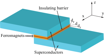
Figure 1: (Color online) Schematic construction of a SFIFS junction of the “overlap”geometry.

II Model and Basic Equations

We consider a planar SFIFS junction of the “overlap” geometry as shown schematically in Fig. 1 (the results obtained are also applicable to an SIFS junction). Our aim is to generalize the equation for the phase difference $\varphi$ between the superconducting layers describing the static and dynamic properties of an SIS JJ to the case of SFIFS JJs.

This equation reads Josephson (1964, 1965); Kulik and Janson (1972); Likharev (1986); Barone and Paternò (1982)

$$\Omega_{J}^{-2}\left(\frac{\partial^{2}\varphi}{\partial t^{2}}+\gamma_{R}\frac{\partial\varphi}{\partial t}\right)-l_{J}^{2}\mathbf{\nabla}_{\perp}^{2}\varphi+\sin(\varphi)=\eta,$$ (1)

where $\Omega_{J}=(2ej_{c}/C_{\Box}\hbar)^{1/2}$ is the Josephson “plasma” frequency, $\gamma_{R}=(R_{\Box}C_{\Box})^{-1}$, $C_{\Box}=\epsilon/4\pi d$, and $R_{\Box}$ are the capacitance and resistance of the junction per unit area, respectively, $d$ is the thickness of the insulating layer, $l_{J}^{2}=v_{J}^{2}/\Omega_{J}^{2}$, $v_{J}=c\sqrt{d/2\epsilon\lambda_{L}}$ is the plasma wave propagation velocity (Swihart waves), $\lambda_{L}$ is the London penetration depth, and $\mathbf{\nabla}_{\perp}$ represents the tangential or in-plane gradient with respect to the interfaces in the $x$-$y$ plane.

We single out the term on the right-hand side of Eq. (1), $\eta=j/j_{c}$, which describes the normalized bias current through the junction. Although it may depend on $y$, the normalized current $\eta$ will be considered as constant along the $y$ direction. Strictly speaking, this is only true for “overlap” junctions Likharev (1986); Barone and Paternò (1982) considered here in which the system geometry is arranged in such a way that the intersection region of superconducting layers is approximately one-dimensional. However, the form of Eq. (1) is most convenient for analysis of CVC for the system under consideration and, moreover, neglecting the $y$ dependence of normalized current $\eta$ does not change qualitatively the final results. The critical current density $j_{c}$ is considered as a known quantity. It was calculated in Refs. Bergeret et al., 2001; Buzdin and Baladié, 2003; Vasenko et al., 2011; Pugach et al., 2011.

The resistance $R_{\Box}$ depends on the voltage $V$ across the junction. This dependence is especially strong in the case of tunnel SIS JJs if the voltage $V$ is close to the energy gap $\Delta$. We assume that the characteristic frequencies ($\Omega_{J}$ and $\Omega_{M}$) are smaller than $\Delta/\hbar$. In addition, we are interested in the form of the CVC at voltages $V$ close to $\hbar\Omega_{J}/2e,\hbar\Omega_{M}/2e$, where $R_{\Box}$ and, therefore, $\gamma_{R}$ can be regarded as constant. Of course, the overall form of the CVC will be modified as a direct consequence of the voltage-dependent damping coefficient $\gamma_{R}(V)$.

We consider planar JJs of the SFIFS, SFIS, or SFS type and assume that the layer separating the two superconductors is characterized by the magnetic susceptibility $\chi(\omega,k)$. In particular, this layer may be a magnetic insulator or metallic ferromagnet. The derivation of an equation for the phase difference $\varphi$ in SFIFS junctions is quite similar to that in the case of tunnel SIS junctions Kulik (1965); Eck et al. (1964); Likharev (1986); Barone and Paternò (1982). We assume that there is no magnetic field normal to the interfaces in the superconductors or, in other words, no Abrikosov vortices pierce the superconducting films, and the lateral dimensions $L_{x,y}$ are much larger than the thickness $d_{F}$ of the F layers and the Josephson penetration depth $\lambda_{L}$. Since the normal component of the magnetic induction $B_{z}$ is continuous at the superconductor-ferromagnet (SF) interfaces, it also vanishes in the ferromagnetic layers and, hence, according to $B_{z}=H_{z}+4\pi M_{z}$ one has $H_{z}=-4\pi M_{z}$ in the F films. In order to find the relation between the magnetic field $H$ in the superconductor (note that in the S layers $H$ coincides with the magnetic induction $B$) and the phase difference $\varphi$, we express the tangential component of the current density in the S film $\mathbf{j}_{\perp}\equiv j_{x}\mathbf{n}_{x}+j_{y}\mathbf{n}_{y}$ using the vector potential $A_{\perp}$ ($\mathbf{n}_{z}\times\partial\mathbf{A}/\partial z=\mathbf{B}_{\perp}$) and the tangential gradient of the phase in the superconductor $\nabla_{\perp}\chi$ as

$$\mathbf{j}_{\perp}=\frac{c}{4\pi\lambda_{L}^{2}}\left(1+\gamma_{qp}\right)\left(-\mathbf{A}_{\perp}-\frac{\Phi_{0}}{2\pi}\mathbf{\nabla}_{\perp}\chi\right),$$ (2)

where $\gamma_{qp}(\omega)=4\pi i\omega\sigma(\omega)\lambda_{L}^{2}/c^{2}$ is a damping parameter describing effects of quasiparticles on the supercurrent and $\Phi_{0}=hc/2e>0$ is the magnetic flux quantum. The parameter $\gamma_{qp}$ is very small for not very high frequencies because the frequency $c/\lambda_{L}$ is very large. For example, taking $\lambda_{L}=5\cdot 10^{-6}\mathrm{cm}$ we obtain $c/\lambda_{L}=0.6\cdot 10^{16}\mathrm{s}^{-1}$, which actually allows us to omit the parameter $\gamma_{qp}$.

Writing Eq. (2) we imply a local relation between the tangential current density $\mathbf{j}_{\perp}$ and the gauge invariant quantity in brackets, which is legitimate in the limit $k\lambda_{L}\ll 1$, where $k$ is the modulus of the in-plane wave vector of perturbations. Subtracting the expressions for the current density, Eq. (2), written for the right and left superconductors from each other we find the change of the tangential current density $[\mathbf{j}_{\perp}]=\mathbf{j}_{\perp}(\widetilde{d}_{F}/2)-\mathbf{j}_{\perp}(-\widetilde{d}_{F}/2)$ across the junction

$$[\mathbf{j}_{\perp}]=\frac{c}{4\pi\lambda_{L}^{2}}\left(1+\gamma_{qp}\right)\left.\left(\widetilde{d}_{F}\left\{\mathbf{n}_{z}\times\mathbf{B}_{\perp}\right\}-\frac{\Phi_{0}}{2\pi}\nabla_{\perp}\varphi\right)\right|_{\frac{\widetilde{d}_{F}}{2}},$$ (3)

where $\widetilde{d}_{F}=d_{F}$ in the case of an SIFS or SFS junction and $\widetilde{d}_{F}=2d_{F}$ in the case of an SFIFS junction. The parameter $d_{F}$ is the thickness of the F film, which is assumed to be smaller than the London penetration length $\lambda_{L}$, and for any quantity $Q$, we denote the difference $Q\big{|}_{S(R)}-Q\big{|}_{S(L)}$ by $[Q]$, where $S(R)$ and $S(L)$ are the right and left superconductors, respectively.

The assumption $d_{F}\ll\lambda_{L}$ allows one to neglect the change of $\mathbf{A}_{\perp}$ along the $z$ direction caused by Meissner currents in the F layer and to write the change of the vector potential $\mathbf{A}_{\perp}$ in the form $[\mathbf{A}_{\perp}]=\widetilde{d}_{F}(\mathbf{n}_{z}\times\mathbf{B}_{\perp})$ with $\mathbf{B}_{\perp}=4\pi\mathbf{M}_{\perp}+\mathbf{H}_{\perp}$. The field $\mathbf{H}_{\perp}$ is approximately the same to the right and to the left from the SF interfaces and does not contribute to the jump of the tangential current density $[\mathbf{j}_{\perp}]$. The Meissner currents in the F layers and, therefore, the variation of $\mathbf{H}_{\perp}$ there are much smaller than in the superconductors for the following reason. The total screening Meissner current $I_{\mathrm{Scr}}$ in the F layer is proportional to $\lambda_{LF}^{-2}\widetilde{d}_{F}\mathbf{A}$, where the inverse London penetration depth $\lambda_{LF}^{-1}$ is proportional to the density of Cooper pairs, $\lambda_{LF}^{-2}\sim n_{SF}$, and, thus, is much smaller than $\lambda_{L}^{-2}$. The phase difference $\varphi$ between the two S layers has the (gauge-invariant) definition:

$$\varphi=[\chi]+\frac{2e}{\hbar c}\int_{S(L)}^{S(R)}dz\,A_{z},$$ (4)

and completely describes the JJ because we choose a gauge with $A_{z}=0$ and $[\chi]=\chi(\widetilde{d}_{F}/2)-\chi(-\widetilde{d}_{F}/2)$.

Equation (3) determines the boundary conditions of the London equation in the superconductors. Indeed, considering the Maxwell equation at the points $z=\pm z_{\mathrm{SF}}\approx\pm\widetilde{d}_{F}/2$,

$$\mathbf{\nabla}\times\mathbf{B}_{\perp}\Big{|}_{\pm\widetilde{d}_{F}/2}=\frac{4\pi}{c}\mathbf{j}_{\perp}\Big{|}_{\pm\widetilde{d}_{F}/2},$$ (5)

where $z_{\mathrm{SF}}$ denotes the coordinate of the right SF interface, we obtain by successively taking the cross product with $\mathbf{n}_{z}$ in both sides and subtracting the two equations from each other

$$-\frac{\partial\mathbf{B}_{\perp}}{\partial z}\Big{|}_{\widetilde{d}_{F}/2}=\frac{2\pi}{c}\mathbf{n}_{z}\times[\mathbf{j}_{\perp}].$$ (6)

Here, we used the relation

$$\left.\frac{\partial\mathbf{B}_{\perp}}{\partial z}\right|_{\widetilde{d}_{F}/2}=-\left.\frac{\partial\mathbf{B}_{\perp}}{\partial z}\right|_{-\widetilde{d}_{F}/2}$$ (7)

taking into account the symmetry of the SFIFS system. Recalling that the magnetic field component $B_{z}$ normal to the interfaces is assumed to be zero in the S layers and considering only the $z$ dependence of $\mathbf{B}_{\perp}$, we have to solve in the superconductors the equation

$$\frac{\partial^{2}\mathbf{B}_{\perp}}{\partial z^{2}}-\kappa^{2}\mathbf{B}_{\perp}=0$$ (8)

with $\kappa^{2}=\lambda_{L}^{-2}\left(1+\gamma_{qp}\right)\approx\lambda_{L}^{-2}$. The solution reads for $|z|~{}>~{}\widetilde{d}_{F}/2$,

$$\mathbf{B}_{\perp}(z)=\mathbf{B}_{\perp}\left(\widetilde{d}_{F}/2\right)\exp\left\{-\frac{|z|-\widetilde{d}_{F}/2}{\lambda_{L}}\right\}.$$ (9)

Inserting this expression for $\mathbf{B}_{\perp}$ into Eq. (6) we obtain by use of Eq. (3)

$$\mathbf{B}_{\perp}\left(\tfrac{\widetilde{d}_{F}}{2}\right)=-\frac{\Phi_{0}}{4\pi\widetilde{\lambda}_{L}}\left(\mathbf{n}_{z}\times\nabla_{\perp}\varphi\right)-\frac{2\pi\widetilde{d}_{F}}{\widetilde{\lambda}_{L}}\mathbf{M}_{\perp}\Big{|}_{\widetilde{d}_{F}/2},$$ (10)

where we have set $\widetilde{\lambda}_{L}=\lambda_{L}+\widetilde{d}_{F}/2$. The magnetic field $B$ decays exponentially with increasing $z$ provided the thickness of the S layers exceeds the London penetration length $\lambda_{L}$.

In order to obtain an equation for the phase difference $\varphi$ of the superconductors we use the Maxwell equation $(\nabla~{}\times~{}\mathbf{H})_{z}~{}-~{}c^{-1}~{}\partial~{}D_{z}/\partial~{}t~{}=~{}(4\pi/c)~{}j_{z}$ and the standard expression for the Josephson current according to the Stewart-McCumber model Stewart (1968); McCumber (1968). This simple model [also known as the resistively and capacitively shunted junction (RCSJ) model] provides a good description of the CVC of a real JJ, although effects due to finite dimensions of the contacts and nonlinearities of the quasiparticle current are neglected. Using the Josephson relation

$$\frac{\partial\varphi}{\partial t}=-\frac{2eV}{\hbar}$$ (11)

and the standard expression for the Josephson current we obtain within this model

$$\frac{c}{4\pi}\left(\nabla\times\mathbf{H}\right)_{z}=-\frac{\hbar C_{\Box}}{2e}\frac{\partial^{2}\varphi}{\partial t^{2}}-\frac{\hbar}{2eR_{\Box}}\frac{\partial\varphi}{\partial t}-j_{c}\sin(\varphi)+j.$$ (12)

Finally, with the help of Eq. (10) and taking into account that in the S layers $B=H$,

$$\Omega_{J}^{-2}\left(\frac{\partial^{2}\varphi}{\partial t^{2}}+\gamma_{R}\frac{\partial\varphi}{\partial t}\right)-l_{J}^{2}\nabla_{\perp}^{2}\varphi+\sin(\varphi)=$$

$$\qquad\qquad\qquad\qquad=\eta+\frac{c\widetilde{d}_{F}}{2\widetilde{\lambda}_{L}j_{c}}\left(\nabla\times\mathbf{M}_{\perp}\right)_{z}$$ (13)

where here, too, $\Omega_{J}=(2ej_{c}/C_{\Box}\hbar)^{1/2}$ is the Josephson “plasma” frequency, $\gamma_{R}=(R_{\Box}C_{\Box})^{-1}$, $C_{\Box}(\omega)=\epsilon(\omega)/4\pi d$ and $R_{\Box}(\omega)$ are the capacitance and resistance of the junction per unit area, respectively, $d$ is the thickness of the insulating layer, $l_{J}^{2}=v_{J}^{2}/\Omega_{J}^{2}$, $v_{J}=c\sqrt{d/2\epsilon\widetilde{\lambda}_{L}}$ is the plasma wave propagation velocity (Swihart waves), and $\eta=j/j_{c}$ is the normalized bias current through the junction. The capacitance $C_{\Box}$ and the resistance $R_{\Box}$ of the junction may depend on frequency $\omega$ (in the Fourier representation). A simpler equation for the phase difference $\varphi$ in the stationary case has been reported previously in Ref. Volkov and Anishchanka, 2005. In a general, non-stationary case, this equation was derived in Ref. Volkov and Efetov, 2009. Note that a slightly different approach for the study of dynamic processes in SFS junctions was used in a recent paper ichi Hikino et al. (2008). In particular, Eq. (13) can be easily derived from Eqs. (A3)–(A6) of this work.

In order to obtain a closed set of equations for the phase difference $\varphi$ of the superconductors and the magnetization $\mathbf{M}_{\perp}$ of the ferromagnetic layer, we need to use a dynamic equation for $\mathbf{M}_{\perp}$ as well.

The dynamics of the magnetization $\mathbf{M}$ in the F layer is described by the well-known Landau-Lifshitz-Gilbert (LLG) equation (see, e.g., Refs. Landau et al., 1984; Aharoni, 1996), which allows one to describe the temporal development of $\mathbf{M}$ in an effective magnetic field $\mathbf{H}_{\mathrm{eff}}$ including all internal and external contributions.

We decompose the magnetization vector $\mathbf{M}$ according to $\mathbf{M}=M_{0}\mathbf{n}_{e}+\mathbf{m}$, where the unit vector $\mathbf{n}_{e}$ denotes the easy axis direction and $\mathbf{m}\perp\mathbf{n}_{e}$ is the dynamic part which evolves in time as described by the LLG equation. Assuming that in equilibrium the magnetization coincides with the static part along the easy axis, i.e. $M_{0}\approx|\mathbf{M}|\gg|\mathbf{m}|$, and using $B_{z}=0$, we obtain

$$\frac{\partial\mathbf{m}}{\partial t} = -4\pi\alpha M_{\mathrm{eff}}\left(1-\widetilde{l}_{M}^{\,2}\nabla_{\perp}^{2}\right)\left(\mathbf{M}\times\mathbf{m}\right)+$$ (14)

$$+M_{\mathrm{eff}}\mathbf{M}\times\mathbf{B}_{\perp}+\frac{\gamma_{M}}{|\mathbf{M}|}\mathbf{M}\times\frac{\partial\mathbf{m}}{\partial t},$$

where $M_{\mathrm{eff}}=g|e|/2mc$, $g<0$ is the gyromagnetic factor, $\alpha$ is a parameter related to the anisotropy constant Landau et al. (1984), $\widetilde{l}_{M}$ is a characteristic length related to spin waves, and $\gamma_{M}$ is the dimensionless Gilbert damping constant.

We further neglect the Gilbert damping term ($\gamma_{M}=0$), align the easy axis along the $z$ direction ($e\equiv z$), and substitute $\mathbf{B}_{\perp F}=4\pi\mathbf{M}_{\perp}+\mathbf{H}_{\perp}$ $(\mathbf{M}_{\perp}\equiv\mathbf{m})$ into Eq. (14), where $\mathbf{B}_{\perp F}$ is the magnetic induction in the F layer and $\mathbf{H}_{\perp}$ is the magnetic field, which is assumed to be independent of the $z$ coordinate (screening effects in the F layer are negligible). The field $\mathbf{H}_{\perp}$ is continuous across the SF interface, i.e., $\mathbf{H}_{\perp}=\mathbf{B}_{\perp}\left(z\rightarrow\widetilde{d}_{F}/2\right)$, and is given by Eq. (10).

Finally, we obtain

$$\frac{\partial\mathbf{m}}{\partial t} = \Omega_{M}\left[\left(1+s-l_{M}^{2}\nabla_{\perp}^{2}\right)\frac{\mathbf{M}\times\mathbf{m}}{M_{0}}-\right.$$ (15)

$$\phantom{\Omega_{M}\Big{[}}\left.\qquad-\frac{\Phi_{0}}{(4\pi)^{2}(\alpha-1)\widetilde{\lambda}_{L}}\nabla_{\perp}\varphi\right],$$

where $\Omega_{M}=4\pi(\alpha-1)|M_{\mathrm{eff}}|M_{0}$ is the resonance frequency of magnetic moment precession ($\alpha>1$), $s=\widetilde{d}_{F}/[2(\alpha-1)\widetilde{\lambda}_{L}]$, $l_{M}^{\,2}=[\alpha/(\alpha-1)]\widetilde{l}_{M}^{2}$.

Equations (13) and (15) fully describe different dynamical processes in the junctions under consideration. Note that the Josephson current is coupled to the magnetization through the spatial derivative of the phase difference $\mathbf{\nabla}_{\perp}\varphi$ [the last term on the right-hand side of Eq. (15)]. Therefore, in a spatially homogeneous case there is no coupling between the Josephson effect and dynamics of the magnetization.

III Fiske steps

In this section, we consider a SFIFS Josephson junction in a weak external magnetic field $H_{\mathrm{ext}}$ assuming that it is constant in space and time and is directed parallel to the interfaces along the $y$ direction. As is well known, in this case so-called Fiske steps arise on the CVC due to excitation of eigenmodes in the junction. The phase difference $\varphi(x,t)$ depends on the $x$ coordinate and, therefore, dynamics of the magnetic and superfluid systems are coupled together. We consider the case when the magnetization vector in the stationary state is directed perpendicular to the SF interfaces, i.e. $\mathbf{M}_{0}=M_{0}\mathbf{n}_{z}$ and $\mathbf{H}_{0}=-4\pi\mathbf{M}_{0}$. As the typical values for the magnitude of the stationary magnetization $M_{0}$ are hundreds of Gauß  and the small external magnetic field $H_{\mathrm{ext}}$ is of the order of a few Gauß, one can neglect the in-plane magnetization $M_{y}=-H_{\mathrm{ext}}/(4\pi)$ compared to $M_{0}$. The resulting precessional motion of the magnetization $\mathbf{M}$ in presence of a current through the JJ implies that the in-plane components $\mathbf{m}\perp\mathbf{n}_{z}$ of $\mathbf{M}$ are excited. Therefore, we represent $\mathbf{M}$ as $\mathbf{M}(x,t)=\mathbf{M}_{0}+\mathbf{m}(x,t)$. Components $m_{x,y}$ are easily found from Eq. (15):

$$m_{y} = \frac{\Omega_{M}(1+s)}{i\omega}m_{x}$$ (16)

$$= \frac{1}{(1+s)\mathcal{L}_{\omega F}}\frac{\Phi_{0}}{(4\pi)^{2}(\alpha-1)\widetilde{\lambda}_{L}}\frac{\partial\varphi}{\partial x},\quad$$

$$\mathcal{L}_{\omega F} = \frac{\omega(\omega-i\gamma_{M})}{\Omega_{M}^{2}(1+s)^{2}}-1.$$ (17)

Equations (16), (17) are written under the assumption that all relevant quantities depend on time as $\exp(i\omega t)$ and, what is more important, spatial derivatives in the equation for $\mathbf{m}(x,t)$ are neglected. The latter assumption is justified provided the magnetic length $l_{M}$ is much shorter than the Josephson length $l_{J}$: $l_{M}\ll l_{J}$. It is not difficult to analyze a more general case of arbitrary relation between $l_{M}$ and $l_{J}$, but the corresponding formulas become too cumbersome. Substituting Eq. (16) into Eq. (13) we obtain

$$-\left[\frac{\omega(\omega-i\gamma_{R})}{\Omega_{J}^{2}}+\widetilde{l}_{J}^{\,2}(\omega)\frac{\partial^{2}}{\partial x^{2}}\right]\varphi(x,\omega)+\qquad\qquad$$ (18)

$$+\mathcal{F}\{\sin(\varphi)\}(x,\omega) = \eta,$$

where $\mathcal{F}\{\sin(\varphi)\}(x,\omega)$ is the Fourier transform of $\sin[\varphi(x,t)]$ with respect to time $t$ and

$$\widetilde{l}_{J}(\omega)=l_{J}\left[1+\frac{s}{(1+s)\mathcal{L}_{\omega F}}\right]^{1/2}$$ (19)

is a renormalized Josephson length containing $\mathcal{L}_{\omega F}$ and, therefore, depending on frequency $\omega$. Equation (18) is the favored generalization of Eq. (1) for SFIFS junctions.

In order to find the CVC, we represent the phase difference $\varphi$ of the superconducting layers in the form $\varphi=\varphi_{0}(x,t)+\psi(x,t)$ (see Ref. Eck et al., 1964). The first term is given by $\varphi_{0}(x,t)=\kappa_{H}x+\Omega_{V}t$ with $\kappa_{H}=4\pi\widetilde{\lambda}_{L}H_{\mathrm{ext}}/\Phi_{0}$ [see Eq. (10)] and $\Omega_{V}=2eV/\hbar$. The function $\psi(x,t)$ is assumed to be small allowing us to linearize Eq. (13) with respect to $\psi$:

$$-\mathit{\widehat{P}}\{\psi\}(x,t) = \sin\left[\varphi_{0}(x,t)\right]$$

$$= \sin(\Omega_{V}t)\cos(\kappa_{H}x)+\cos(\Omega_{V}t)\sin(\kappa_{H}x)$$

where the operator $\mathit{\widehat{P}}$ is defined as

$$\mathit{\widehat{P}}=\Omega_{J}^{-2}\left(\frac{\partial^{2}}{\partial t^{2}}+\gamma_{R}\frac{\partial}{\partial t}\right)-\widetilde{l}_{J}^{\,2}(\Omega_{V})\frac{\partial^{2}}{\partial x^{2}}.$$ (21)

The current correction $\delta\eta$ to the dc current $\eta_{0}=(2eV/\hbar)/\Omega_{J}=\Omega_{V}/\Omega_{J}$ is given by

$$\delta\eta=\big{\langle}\psi(x,t)\cos\left[\varphi_{0}(x,t)\right]\big{\rangle},$$ (22)

where the angular brackets denote the average with respect to space and time.

Equation (22) determines the constant normalized current through the junction as a function of voltage $V$, which gives a current-voltage (I-V) curve. Equation (III) contains parts oscillating in space and time. It should be solved taking into account the boundary conditions Eck et al. (1964); Kulik (1965); Likharev (1986); Barone and Paternò (1982)

$$\left.\frac{\partial\psi}{\partial x}\right|_{x=\pm L}=0,$$ (23)

where $L$ denotes the length of the junction along the $x$ direction. The right-hand side of Eq. (III) can be written in the form $\mathrm{Im}\{\exp(i\Omega_{V}t)[\cos(\kappa_{H}x)+i\sin(\kappa_{H}x)]\}$ and, therefore, the solution of Eq. (III) can be written as $\psi(x,t)=\mathrm{Im}\{\exp(i\Omega_{V}t)\psi_{1}(x)\}$, where the function $\psi_{1}(x)$ obeys the equation

$$-\mathit{\widehat{P}}_{\Omega}\{\psi_{1}\}(x)=\cos(\kappa_{H}x)+i\sin(\kappa_{H}x)$$ (24)

with the boundary condition Eq. (23).

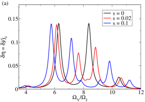
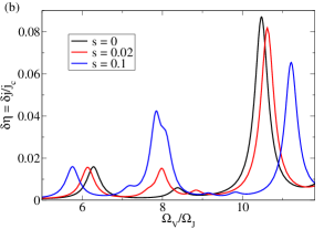
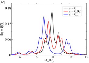
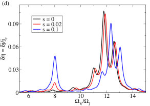
Figure 2: (Color online) Correction to the $I$-$V$ characteristics of an SFIFS JJ in a weak external magnetic field due to interaction of Josephson oscillations and spin-wave modes. The correction is plotted as a function of normalized voltage $V_{\mathrm{norm.}}=\Omega_{V}/\Omega_{J}$ for different values of the parameter $s$. The figures are presented for the following parameters: (a) $\Omega_{M}/\Omega_{J}=\kappa_{H}l_{J}=8$ and $L/l_{J}=0.75$, (b) $\Omega_{M}/\Omega_{J}=8,\kappa_{H}l_{J}=12,L/l_{J}=0.75$; (c) $\Omega_{M}/\Omega_{J}=\kappa_{H}l_{J}=8,L/l_{J}=2$; (d) $\Omega_{M}/\Omega_{J}=8,\kappa_{H}l_{J}=12,L/l_{J}=2$. The damping coefficients are $\gamma_{R}/\Omega_{J}=0.4,\gamma_{M}/\Omega_{J}=0.3$.

The operator $\mathit{\widehat{P}}_{\Omega}$ coincides with $\mathit{\widehat{P}}$ after replacing $\partial/\partial t$ by $i\Omega_{V}$. The solution can be easily found and equals

$$\psi_{1} = \frac{1}{\mathit{P}_{\Omega}(V,H)}\Big{\{}\cos(\kappa_{H}x)+C\cos(\kappa_{V}x)+i\sin(\kappa_{H}x)+$$ (25)

$$\phantom{\frac{1}{\mathit{\widehat{P}}_{\Omega}(V,H)}\{}+iS\sin(\kappa_{V}x)\Big{\}}$$

where $\mathit{P}_{\Omega}(V,H)=a^{2}-\widetilde{l}_{J}^{\,2}(\Omega_{V})\kappa_{H}^{2}$, $a^{2}=\Omega_{J}^{-2}(\Omega_{V}^{2}-i\gamma_{R}\Omega_{V})$ and

$$C=-\frac{\theta_{H}}{\theta_{V}}\frac{\sin\theta_{H}}{\sin\theta_{V}},\quad S=-\frac{\theta_{H}}{\theta_{V}}\frac{\cos\theta_{H}}{\cos\theta_{V}}$$ (26)

with $\theta_{H}=\kappa_{H}L,\,\theta_{V}=\kappa_{V}L,\,\kappa_{V}^{2}=a^{2}\widetilde{l}_{J}^{\,-2}(\Omega_{V})$. Substituting the function $\psi(x,t)$ expressed through $\psi_{1}(x)$ into Eq. (22), we find the dependence, $\delta\eta(V)\equiv\delta j(V)/j_{c}$,

$$\delta\eta = \mathrm{Im}\left\{\frac{1}{\mathit{P}_{\Omega}(V,H)}\left[1-\frac{\theta_{H}^{2}}{\theta_{V}\left(\theta_{H}^{2}-\theta_{V}^{2}\right)}\times\right.\right.$$ (27)

$$\phantom{\mathrm{Im}\Big{\{}\frac{1}{\mathit{\widehat{P}}_{\Omega}(V,H)}}\times\left.\left.\frac{\cos(2\theta_{V})-\cos(2\theta_{H})}{\sin(2\theta_{V})}\right]\right\}.$$

Since we assumed that the correction $\psi=\mathrm{Im}\left\{\exp\left(i\Omega_{V}t\right)\psi_{1}(x)\right\}$ to the phase difference $\varphi$ in the superconducting layers is small, Eq. (27) is only valid for normalized voltages $\Omega_{V}/\Omega_{J}>(\gamma_{R}/\Omega_{J})^{-1}$. This can be seen from Eq. (25) where one should verify that the prefactor $P_{\Omega}^{-1}(V,H)$ is small.

Let us discuss the current results and compare them with those obtained in Ref. Volkov and Efetov, 2009. The prefactor $P_{\Omega}^{-1}(V,H)$ in Eq. (27) contains the renormalized Josephson length $\widetilde{l}_{J}$ defined in Eq. (19), which corresponds to the quantity $l_{V}$ of Ref. Volkov and Efetov, 2009. The formulas for Fiske steps in Ref. Volkov and Efetov, 2009 were given for small values of the parameter $s$. If the parameter $s$ is not very small, one can reproduce the correct result by replacing there $\Omega_{M}^{2}\rightarrow(1+s)\Omega_{M}^{2}$, i.e., Eq. (19). [Note that in the definition of $\Omega_{Ms}$, Eq. (10) of Ref. Volkov and Efetov, 2009, there is a misprint. The factor of two in the exponent at the right-hand side is missing so that the correct formula reads $\Omega_{Ms}^{2}=\Omega_{M}^{2}(1+s)^{2}$.] The modified dependence of the normalized Josephson length $\widetilde{l}_{J}$ on the parameter $s$ changes the form of the $I$-$V$ characteristics and reveals that the effect of the ferromagnetic layer is much more pronounced compared to the results of Ref. Volkov and Efetov, 2009 even for small $s$ because the denominator in Eq. (10) of Ref. Volkov and Efetov, 2009 is very small at voltages corresponding to peaks in the CVC and, therefore, is very sensitive to the parameter $s$. Thus, we update the figures showing the dependence $\delta\eta(V_{\mathrm{norm.}})$ as a function of normalized voltage $V_{\mathrm{norm.}}=\Omega_{V}/\Omega_{J}$. Finally, we also present $I$-$V$ characteristics for different values of normalized junction lengths $L/l_{J}$ including those which correspond to the experimental values of Ref. Wild, G. et al., 2010 ($L/l_{J}<1$). As in Ref. Volkov and Efetov, 2009, for simplicity, we assume that the damping coefficient $\gamma_{R}$ is constant, i.e., it does not depend on voltage $V$.

In Figs. 2 and 3, we plot the current correction $\delta\eta$ as a function of normalized voltage $V_{\mathrm{norm.}}$ for different values of the parameter $s=\widetilde{d}_{F}/(2(\alpha-1)\widetilde{\lambda}_{L})$ and normalized junction length $L/l_{J}$. Taking into account the experimental values of $L$ and $l_{J}$ (see Ref. Wild, G. et al., 2010), we display the current correction $\delta\eta$ for short junctions with $L/l_{J}=0.75$ [see Figs. 2(a) and 2(b)] and, in addition, for longer junctions with $L/l_{J}=2$ [see Figs. 2(c) and 2(d)] and $L/l_{J}=10$ [see Figs. 3(a) and 3(b)]. Black curves represent the limit $s\rightarrow 0$ where we have no F layers in the system and the CVC correspond to ordinary Fiske steps. Due to the fact that in experiments, only the strength of the external magnetic field can be varied, we display our result for different values of the parameter $\kappa_{H}l_{J}\propto H_{\mathrm{ext}}$ keeping all other system parameters such as $\Omega_{M}/\Omega_{J},L/l_{J}$, and $s$ constant.

The strongest influence of the ferromagnetic layers on the current-voltage characteristics develops for external magnetic fields such that the parameters $\kappa_{H}l_{J}$ and $\Omega_{M}/\Omega_{J}$ coincide. By comparing Figs. 2(a) and 2(b) [or Figs. 2(c) and 2(d), respectively] one can observe that the change of the current correction is clearly recognizable for $\kappa_{H}l_{J}=\Omega_{M}/\Omega_{J}$ and nonzero $s$, while for $\kappa_{H}l_{J}\neq\Omega_{M}/\Omega_{J}$, it only becomes pronounced for larger values of $s$.

As can be seen from Figs. 2(a) and 2(c) that the normalized junction length $L/l_{J}$ determines the form of the CVC even in the case $s=0$, i.e., the number of Fiske steps close to the normalized magnetic resonance frequency $\Omega_{M}/\Omega_{J}$ may vary for different values of $L/l_{J}$. Provided for $s=0$ there appears a single peak close to $\Omega_{M}/\Omega_{J}$, increasing the parameter $s$ leads to a double splitting of the dominant peak. For even larger values of $s$, the pair of peaks moves more and more apart from each other [see Fig. 2(a)]. A similar effect can be seen for a larger number of Fiske steps close to $\Omega_{M}/\Omega_{J}$, e.g., Fig. 2(c) displays essentially two Fiske steps in the vicinity of $\Omega_{M}/\Omega_{J}=8$ that both split up into two peaks moving apart from each other with increasing $s$.

For distinct values of the parameters $\kappa_{H}l_{J}$ and $\Omega_{M}/\Omega_{J}$ [see Figs. 2(b) and 2(d)], there also emerge additional peaks in the $I$-$V$ characteristics close to the normalized magnetic resonance frequency, but the detailed impact of the F layers on the CVC is not as obvious as is the case for $\kappa_{H}l_{J}=\Omega_{M}/\Omega_{J}$. From Fig. 2(d), one can already conjecture that for long junctions, the ferromagnetic layers simply induce a single additional peak close to $\Omega_{M}/\Omega_{J}$. In Fig. 3, where the current correction $\delta\eta$ is shown for the limit of large values of $L/l_{J}$ ($L/l_{J}=10$), this feature becomes more apparent. For coinciding values of the magnetic resonance frequency $\Omega_{M}/\Omega_{J}$ and the parameter $\kappa_{H}l_{J}$ [see Fig. 3(a)], we find a single peak for $s=0$ and a double peak for $s\neq 0$ in the vicinity of $\Omega_{M}/\Omega_{J}$. For $\Omega_{M}/\Omega_{J}\neq\kappa_{H}l_{J}$, there emerges a single peak close to $\Omega_{M}/\Omega_{J}$ and $\kappa_{H}l_{J}$, respectively, where the former is notably smaller in magnitude [see Fig. 3(b)]. Below we also derive analytical expressions for these peak positions.

Thus the presence of the F layers leads not only to a shift of the peaks in the dependence $\delta\eta(V_{\mathrm{norm.}})$ but also to a change of the overall form of this dependence. The additional peaks arising on the $I$-$V$ curves can be attributed to the ferromagnetic resonance and the nonzero coupling between Josephson and magnetic moment oscillations. In order to observe these peaks experimentally, one should perform measurements with different samples that contain ferromagnetic layers of varying thickness. Then, according to our theoretical result, one would be able to differentiate between ordinary Fiske steps and peaks caused by interaction of Josephson and magnetic oscillations in the F layers.

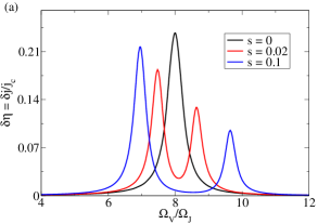
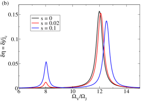
Figure 3: (Color online) Current correction $\delta\eta$ as a function of normalized voltage $V_{\mathrm{norm.}}=\Omega_{V}/\Omega_{J}$ for long JJ with normalized junction length $L/l_{J}=10$. The function $\delta\eta$ is displayed for (a) $\Omega_{M}/\Omega_{J}=\kappa_{H}l_{J}=8$; (b) $\Omega_{M}/\Omega_{J}=8,\kappa_{H}l_{J}=12$ and for different values of the parameter $s$. The damping coefficients are $\gamma_{R}/\Omega_{J}=0.4,\gamma_{M}/\Omega_{J}=0.3$.

Note that in the limit of a very short junction ($L/l_{J}\ll 1$) there is no coupling between Josephson and magnetic moment oscillations. Indeed, in this limit we obtain from Eq. (27)

$$\delta\eta=\mathrm{Im}\left\{\frac{\Omega_{J}^{2}}{\Omega_{V}\left(\Omega_{V}-i\gamma_{R}\right)}\right\}.$$ (28)

It is seen that magnetic characteristics such as $\Omega_{M}$ of the F layers drop out from this expression.

In the limit of long junctions, $L/l_{J}\gg 1$, the expression for the current correction can be approximated by

$$\delta\eta = \mathrm{Im}\left\{\frac{1}{P_{\Omega}(V,H)}\right\}$$

$$= \mathrm{Im}\left\{\frac{\Omega_{V}^{2}-i\gamma_{R}\Omega_{V}}{\Omega_{J}^{2}}-\kappa_{H}^{2}l_{J}^{2}\left[1+\frac{s}{(1+s)\mathcal{L}_{\Omega_{V}F}}\right]\right\}^{-1}.$$

In accordance to Fig. 3 we obtain for $s=0$ a single peak at normalized voltage $V_{\mathrm{norm.}}=\kappa_{H}l_{J}$ while for $s\neq 0$ and $\kappa_{H}l_{J}=\Omega_{M}/\Omega_{J}$ there exist two peaks at

$$V_{\mathrm{norm.}}=\frac{\Omega_{M}}{\Omega_{J}}\sqrt{(1+s)\pm\sqrt{s(1+s)}}.$$ (30)

Finally, for the general case $s\neq 0$ and $\kappa_{H}l_{J}\neq\Omega_{M}/\Omega_{J}$ we find in leading order in the parameter $s$ two peaks located at normalized voltages

$$V_{\mathrm{norm.}}^{(1)} = \kappa_{H}l_{J}\sqrt{1+s\cdot\frac{x^{2}}{1-x^{2}}}$$ (31a)

$$V_{\mathrm{norm.}}^{(2)} = \frac{\Omega_{M}}{\Omega_{J}}\sqrt{1+s\cdot\frac{1-2x^{2}}{1-x^{2}}}$$ (31b)

where $x=(\Omega_{M}/\Omega_{J})/(\kappa_{H}l_{J})$. These analytical expressions perfectly describe the peak locations of the current-voltage characteristics in the limit $L/l_{J}\gg 1$ as exemplarily shown in Fig. 3 for junctions with $L/l_{J}=10$.

IV Coupled Collective Modes

In this section, we analyze the spectrum of coupled collective modes in long Josephson junctions with a ferromagnetic layer. So far we have derived essentially two (coupled) equations, Eqs. (13) and (15), that describe respectively the dynamics of the phase difference $\varphi$ of the S layers and the magnetization $\mathbf{M}$ of the ferromagnetic layers. Here, we consider again the case when the magnetization $\mathbf{M}_{0}$ is aligned normal to the interface so that in equilibrium $\mathbf{B}_{0}=0$. Small perturbations near the equilibrium result in precessional motion of the magnetic moment $\mathbf{M}$ and in a variation of the phase difference $\varphi$ in space and time. In order to find the spectrum of collective modes in the system, we represent the phase difference $\varphi$ and the magnetic moment $\mathbf{M}$ in the form

$$\varphi=\varphi_{0}+\psi,\quad\mathbf{M}=M_{0}\mathbf{n}_{z}+\mathbf{m}_{\perp},$$ (32)

where $\mathbf{n}_{z}$ is the unit vector normal to the SF interface and the functions $\psi$ and $\mathbf{m}_{\perp}$ are assumed to be small, $|\psi|\ll|\varphi_{0}|$ and $|\mathbf{m}_{\perp}|\ll|M_{0}|$. Linearizing Eq. (13) with respect to $\psi$, we find that the function $\psi(x,t)$ obeys the equation

$$\Omega_{J}^{-2}\left(\frac{\partial^{2}\psi}{\partial t^{2}}+\gamma_{R}\frac{\partial\psi}{\partial t}\right)-l_{J}^{2}\nabla_{\perp}^{2}\psi+\psi=$$ (33)

$$\qquad\qquad\qquad\qquad\qquad\qquad=\frac{c\widetilde{d}_{F}}{2\widetilde{\lambda}_{L}j_{c}}\Big{[}\nabla\times\mathbf{m}_{\perp}\Big{]}_{z}.$$

The perturbation $\mathbf{m}_{\perp}$ of the magnetic moment is parallel to the SF interface and is described by the equation

$$\frac{\partial\mathbf{m}_{\perp}}{\partial t} = \Omega_{M}\Bigg{\{}\left(1+s-l_{M}^{2}\nabla_{\perp}^{2}\right)\Big{[}\mathbf{n}_{z}\times\mathbf{m}_{\perp}\Big{]}-$$

$$\phantom{\Omega_{M}\Bigg{\{}}-\frac{\Phi_{0}}{(4\pi)^{2}\beta\widetilde{\lambda}_{L}}\nabla_{\perp}\psi\Bigg{\}}+\gamma_{M}\left[\mathbf{n}_{z}\times\frac{\partial\mathbf{m}_{\perp}}{\partial t}\right],$$

where we included again the Gilbert damping term, which was neglected in Eq. (15). Fourier transforming the perturbations $\varphi(\mathbf{r},t)$ and $\mathbf{m}_{\perp}(\mathbf{r},t)$ to $(\mathbf{k}_{\perp},\omega)$ representation and combining Eqs. (33) and (IV) into a single equation, we obtain

$$\mathcal{M}\left(\begin{array}[]{c}\varphi(\mathbf{k}_{\perp},\omega)\\ \mathbf{m}_{\perp}(\mathbf{k}_{\perp},\omega)\end{array}\right)=0,$$ (37)

$$\mathcal{M}=\begin{pmatrix}\Omega_{J}^{-2}\left(\omega_{J}^{2}-\omega^{2}\right)&ibk_{y}&-ibk_{x}\\ iak_{x}&-i\omega&\omega_{M}\\ iak_{y}&-\omega_{M}&-i\omega\end{pmatrix},$$ (38)

where $\omega_{J}^{2}\equiv\omega_{J}^{2}(k,\omega)=\Omega_{J}^{2}\left(1+k^{2}l_{J}^{2}\right)-i\gamma_{R}\omega,\,\omega_{M}\equiv\omega_{M}(k,\omega)=\Omega_{M}\left(1+s+k^{2}l_{M}^{2}\right)-i\gamma_{M}\omega$, $b=s\beta c/j_{c}$, $a=s\Omega_{M}l_{J}^{2}/b$, and $k=|\mathbf{k}_{\perp}|$.

The homogeneous equation (37) has a non-vanishing solution provided the determinant of $\mathcal{M}$ equals zero. Setting $\mathrm{det}(\mathcal{M})$ equal to zero we obtain the dispersion relation

$$\left[\omega^{2}-\omega_{J}^{2}\right]\left[\omega^{2}-\omega_{M}^{2}\right]=sv_{J}^{2}\Omega_{M}\omega_{M}k^{2}.$$ (39)

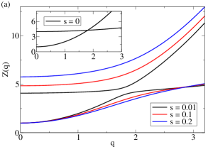
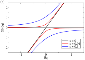
Figure 4: (Color online) Spectrum of coupled spin and plasma-like modes. (a) The function $Z(q)=(\omega(q)/\Omega_{J})^{2}$ determined by Eq. (42) is shown for finite values of $s$ and in the inset for the case $s=0$. (b) The dependence $\delta Z(\delta q)$ that represents the spectrum close to the crossing point is plotted according to Eq. (41). The following parameters are chosen: $Z_{M}=(\Omega_{M}/\Omega_{J})^{2}=4,\,l_{M}/l_{J}=0.1$.

From Eq. (39) we can conclude that the spin and charge excitations decouple only in the limit when the right-hand side of this equation can be neglected. In this case the spin waves with spectrum $\omega_{M}(k,\omega)$ and the plasmalike Josephson waves with spectrum $\omega_{J}(k,\omega)$ exist separately. In the general case, Eq. (39) describes the spectrum of coupled spin waves and plasma-like modes in the system. The most interesting behavior corresponds to the case $\Omega_{M}>\Omega_{J}$. In this situation, the two branches of the spectrum cross each other in the absence of the coupling, while a finite coupling leads to mutual repulsion of these branches.

In order to show this explicitly, we consider the case without damping, $\gamma_{R}=\gamma_{M}=0$, and assume that $s\ll 1$ and $l_{M}\ll l_{J}$, which means that we neglect the spatial dispersion of spin waves on the Josephson length (these conditions are usually fulfilled experimentally). It is convenient to write Eq. (39) in the dimensionless form

$$\left[Z-1-q^{2}\right]\left[Z-Z_{M}\right]=sq^{2}Z_{M},$$ (40)

where $Z=(\omega/\Omega_{J})^{2},\,Z_{M}=(\Omega_{M}/\Omega_{J})^{2}$ and $q=l_{J}k$. One can see that for $s=0$ the two dispersion curves $Z=1+q^{2}$ and $Z=Z_{M}$ cross each other at $q_{0}^{2}=Z_{M}-1$. To find the form of the dispersion curve in the vicinity of the crossing point $q_{0}$, we represent $Z$ and $q$, respectively, as $Z=Z_{M}+\delta Z$ and $q=q_{0}+\delta q$. Then, one can easily obtain from Eq. (40)

$$\delta Z=q_{0}\left[\delta q\pm\sqrt{\delta q^{2}+sZ_{M}}\right].$$ (41)

In Fig. 4 we plot the spectrum of coupled spin and plasma-like modes and the function $\delta Z(\delta q)$ close to the crossing point. Here, we take into account a finite value of the parameter $l_{M}/l_{J}$ so that Eq. (40) that determines the function $Z(q)$ takes the form

$$\left[Z-1-q^{2}\right]\left[Z-\widetilde{Z}_{M}\right]=sq^{2}\sqrt{\widetilde{Z}_{M}}Z_{M},$$ (42)

with $\widetilde{Z}_{M}=Z_{M}[1+s+q^{2}(l_{M}/l_{J})^{2}]^{2}$. The inset of Fig. 4(a) indicates that the two branches indeed cross each other for $s=0$, whereas for $s\neq 0$ we find a “repulsion”of the spin and Josephson excitations. Figure 4(b) displays the function $\delta Z(\delta q)$ that represents the behavior of the spectrum in the vicinity of the crossing point and distinctly emphasizes the mutual repulsion. Both the dispersion curves $Z(q)$ and $\delta Z(\delta q)$ given by Eqs. (41) and (42), respectively, are presented for several values of $s$ and the parameters $\Omega_{M}/\Omega_{J}=2,\,l_{M}/l_{J}=0.1$.

V Ferromagnetic Resonance

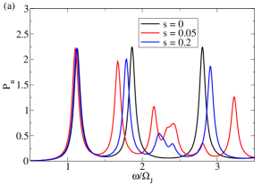
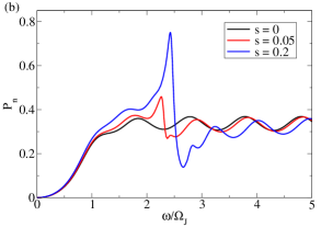
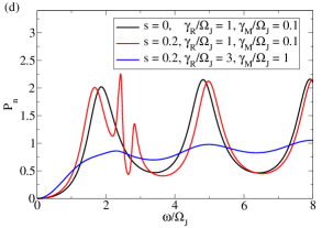
Figure 5: (Color online) Frequency dependence of the normalized absorbed power $\mathcal{P}_{n}$ in the JJ as a function of the normalized frequency $\omega/\Omega_{J}$ for different values of the parameter $s$ and for different damping coefficients $\gamma_{R}/\Omega_{J}$ and $\gamma_{M}/\Omega_{J}$. The figures (a) and (b) are shown for the parameters $L_{n}=3,\gamma_{M}/\Omega_{J}=0.1,(\Omega_{M}/\Omega_{J})^{2}=5$ and, respectively, (a) $\gamma_{R}/\Omega_{J}=0.1$, (b) $\gamma_{R}/\Omega_{J}=1$. With regard to figures (c) and (d) we have chosen $L_{n}=1,(\Omega_{M}/\Omega_{J})^{2}=5$ and in (c) $\gamma_{M}/\Omega_{J}=0.1$.

In this section, we study the response of the system to an external oscillating magnetic field $H_{\mathrm{ext}}(t)=H_{\nu}\sin(\nu t)$ with a small amplitude $H_{\nu}\ll M_{0}$ and frequency $\nu$. The applied field is supposed to be directed along the $y$ axis, i.e., $\mathbf{H}_{\mathrm{ext}}(t)=H_{\mathrm{ext}}(t)\mathbf{n}_{y}$. We assume again that the equilibrium magnetization $\mathbf{M}_{0}$ is oriented in the $z$ direction, $\mathbf{M}=M_{0}\mathbf{n}_{z}$. The external magnetic field $H_{\mathrm{ext}}(t)$ causes precessional motion of the magnetization vector $\mathbf{M}$ and a variation of the phase difference $\varphi$ in space and time. As before (see Sec. III), we, respectively, represent magnetization and phase difference in the form $\mathbf{M}(x,t)=M_{0}\mathbf{n}_{z}+m_{y}(x,t)\mathbf{n}_{y}$ and $\varphi(x,t)=\varphi_{0}+\psi(x,t)$. Here, $\varphi_{0}$ is a constant determined by a bias current $j_{b}=j_{c}\sin(\varphi_{0})$ and $\psi(x,t),\,m_{y}(x,t)$ are small perturbations due to the external ac magnetic field $H_{\mathrm{ext}}(t)=H_{\nu}\,\mathrm{Im}\left[\exp(i\nu t)\right]$, $|\psi|\ll|\varphi_{0}|,\,|m_{y}|\ll|M_{0}|$. Due to the coupling of $\mathbf{M}$ and $\varphi$, we expect modifications of the ferromagnetic resonance in the system appearing as additional features in absorption spectra.

Thus, to study ferromagnetic resonance, we need to calculate the power $\mathcal{P}$ (per unit area) absorbed in the system. The absorbed power $\mathcal{P}$ can be found as the time-averaged difference between the energy flux $\mathcal{S}_{\mathrm{in,out}}$ coming in and out of the system. These fluxes are expressed in terms of Poynting vectors $\mathcal{S}$Landau et al. (1984)

$$\mathcal{P}=\int dzdy\,\mathbf{n}_{x}\cdot\left\langle\mathcal{S}_{\mathrm{in}}-\mathcal{S}_{\mathrm{out}}\right\rangle,$$ (43)

where $\mathcal{S}_{\mathrm{in,out}}=(c/4\pi)[\mathbf{E}\times\mathbf{H}]_{x=\pm L}$ and the angular brackets denote averaging with respect to time $t$.

The electric field $\mathbf{E}=\mathbf{n}_{z}E$ is directed along the $z-$axis and is related to the time derivative of the phase difference via the Josephson relation

$$E=-(1/d)(\hbar/2e)\partial\psi/\partial t.$$ (44)

Therefore, in order to find the Poynting vector $\mathcal{S}$, we have to calculate the function $\psi(t)$ which is determined by an applied weak ac magnetic field $H_{\mathrm{ext}}(t)$. This vector $\mathcal{S}$ differs from zero only in the insulating layer of thickness $d$. The magnetic field consists only of the applied ac field, $\mathbf{H}(x=\pm L)=H_{\mathrm{ext}}(t)\mathbf{n}_{y}$ and, therefore, the Poynting vectors are directed parallel to the $x-$axis. We represent the phase difference in form of the Fourier transform $\psi(x,t)=\int d\omega/(2\pi)\exp(i\omega t)\psi(x,\omega),\,\psi(x,-\omega)=\psi^{\ast}(x,\omega)$.

The function $\psi(x,\omega)$ obeys an equation that is derived in a way similar to the derivation of Eqs. (18)–(22) and has the form

$$\frac{\partial^{2}}{\partial x_{n}^{2}}\psi(x_{n},\omega)-\kappa_{\omega}^{2}\psi(x_{n},\omega)=0,$$ (45)

where we have introduced the dimensionless variable $x_{n}=x/l_{J}$ and have set

$$\kappa_{\omega}^{2}=\frac{\mathcal{L}_{\omega J}}{1+s/[(1+s)\mathcal{L}_{\omega F}]}\equiv\frac{\mathcal{L}_{\omega J}}{a_{\omega}}$$ (46)

with $\mathcal{L}_{\omega J}~{}\equiv~{}\cos(\varphi_{0})~{}-~{}\omega(\omega-i\gamma_{R})/\Omega_{J}^{2}$,  $a_{\omega}~{}=~{}1+s/[(1+s)\mathcal{L}_{\omega F}]$, and $\mathcal{L}_{\omega F}$ is defined in Eq. (17).

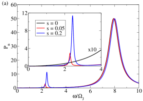
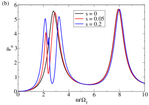
Figure 6: (Color online) Frequency dependence of the normalized absorbed power $\mathcal{P}_{n}$ as a function of the normalized frequency $\omega/\Omega_{J}$ for really short junctions. Here, too, the figures are displayed for different values of the parameter $s$ and for the choice $\gamma_{R}/\Omega_{J}=1,\gamma_{M}/\Omega_{J}=0.1,(\Omega_{M}/\Omega_{J})^{2}=5$. In figure (a) $L_{n}=0.2$ whereas in figure (b) $L_{n}=0.6$.

Equation (46) is supplemented by the boundary conditions

$$\left.a_{\omega}\frac{\partial}{\partial x_{n}}\psi(x,\omega)\right|_{x=\pm L}=-\frac{H_{\mathrm{ext}}(\omega)}{H_{0}}\,\mathrm{and}\,H_{0}=\frac{\Phi_{0}}{4\pi\widetilde{\lambda}_{L}l_{J}}$$ (47)

that can be obtained from Eqs. (9) and (10). As a consequence, the solution for Eq. (45) has the form

$$\psi(\pm L,\omega)=\mp\frac{H_{\mathrm{ext}}(\omega)L_{n}}{H_{0}}\frac{\tanh(\theta_{\omega})}{a_{\omega}\theta_{\omega}}$$ (48)

where $\theta_{\omega}=\kappa_{\omega}L_{n}\equiv\theta_{\omega}^{\prime}+i\theta_{\omega}^{\prime\prime},\,L_{n}=L/l_{J}$. Fourier transforming Eq. (48) back into the time representation we obtain

$$\psi(\pm L,t)=\mp\frac{H_{\nu}L_{n}}{H_{0}}\mathrm{Re}\left[\frac{e^{i\nu t}}{a_{\nu}\theta_{\nu}}\tanh(\theta_{\nu})\right].$$ (49)

Taking into account that all the quantities do not depend on $y$, the absorbed power $\mathcal{P}$ can be represented as

$$\mathcal{P}=2L_{y}\frac{\hbar c}{4\pi e}\left\langle\frac{\partial\psi(L,t)}{\partial t}H_{\mathrm{ext}}(t)\right\rangle,$$ (50)

where $L_{y}$ is the length of the junction along the $y$ direction. Substituting Eq. (49) into Eq. (50) and relabeling the external field frequency $\nu\rightarrow\omega$, we finally arrive at

$$\mathcal{P}=\frac{\Phi_{0}H_{0}}{(2\pi)^{2}}\left(\frac{H_{\omega}}{H_{0}}\right)^{2}\frac{L_{x}L_{y}}{l_{J}}\,\omega\,\,\mathrm{Im}\left[\frac{\tanh\left(\theta_{\omega}\right)}{a_{\omega}\theta_{\omega}}\right],$$ (51)

where $L_{x}\equiv L$. This formula differs drastically from a standard formula for the absorbed power $\mathcal{P}$ in ferromagnetic films because it describes the power absorption not only in the F film, but also in the Josephson junction. In particular, $\mathcal{P}\neq 0$ even in the absence of the ferromagnetic layer. In this case, Eq. (51) describes the power needed to excite standing plasma waves.

In Fig. 5, we plot the frequency dependence of the normalized absorbed power $\mathcal{P}_{n}=(\omega/\Omega_{J})\mathrm{Im}\left[\tanh(\theta_{\omega})/(a_{\omega}\theta_{\omega})\right]$ as a function of normalized frequency $\omega/\Omega_{J}$ at different $s$ and normalized junction length $L/l_{J}$. Generally speaking, from Fig. 5(a), we see that at $s=0$ (no ferromagnetic layer), there are periodic resonances related to excitation of standing waves in the Josephson junction (Josephson plasma resonances). Interestingly, in the presence of the ferromagnetic layers, $s\neq 0$, additional peaks appear on the curves. These peaks are caused by the ferromagnetic resonance in the F layer at frequencies $\omega\approx\Omega_{M}$. With increasing $s$ the influence of the F layer becomes more and more pronounced. One can see this from the fact that, for instance, the spectrum close to $\omega\approx\Omega_{M}$ appears to have a more complicated structure and the peaks increase in height.

To indicate the influence of the (normalized) damping parameters $\gamma_{R}$ and $\gamma_{M}$, we display in Fig. 5(b) the normalized absorbed power $P_{n}$ for the case $\gamma_{R}\gg\gamma_{M}$. This shows that the periodic resonances in the junction are strongly suppressed and the absorption spectrum is dominated by the effect of the ferromagnetic layer. In addition to that, the normalized length of the junction $L_{n}=L_{x}/l_{J}$ also determines the absorption spectrum. In Figs. 5(c) and 5(d), $P_{n}$ is shown for the case $L_{n}~{}=~{}1$ and here, too, for different values of the parameters $s,\gamma_{R},$ and $\gamma_{M}$. We find that the distance between periodic resonances is larger for short junctions and compared to Fig. 5(a), where $L_{n}~{}=~{}3$, the influence of the F layer on the absorption spectrum is weaker. The blue curve in Fig. 5(c) reveals that the periodic resonances can be almost completely suppressed by increasing the damping parameter $\gamma_{R}$. Eventually, Fig. 5(d) indicates that in systems where both damping parameters $\gamma_{R}$ and $\gamma_{M}$ are large and of the same order of magnitude, the effect of the ferromagnetic layer becomes negligible.

In Fig. 6, we show the frequency dependence of the absorbed power $P_{n}$ for short junctions of length $L_{n}=0.2$ [see Fig. 6(a)] and $L_{n}=0.6$ [see Fig. 6(b)]. In Fig. 6(a), the peak at $\omega/\Omega_{J}\approx 2.3$ is related to the ferromagnetic resonance in the F film. In contrast to this, slightly longer junctions feature a much stronger influence of the ferromagnetic layer as becomes apparent from Fig. 6(b). More importantly, we find that the relative magnitudes of peaks due to the Josephson plasma resonances and the ferromagnetic resonance are even in the case of $\gamma_{R}\gg\gamma_{M}$ of the same order of magnitude for short junctions contrary to Fig. 5(b), $L_{n}=3$, where the Josephson plasma resonances are considerably smaller for the same choice of parameters.

Note that our analysis is valid for not too high frequencies as it is assumed that the penetration depth is not frequency dependent. This means that the inequality $\omega\ll\Omega_{J}l_{J}/\lambda_{L}=v_{J}/\lambda_{L}$ should be fulfilled. For this reason, Figs. 6(a) and 6(b) indicate only a small number of Josephson plasma resonances.

VI Discussion

We studied dynamic properties of Josephson junctions with a magnetically active layer characterized by the magnetic susceptibility $\chi(\omega,k)$. These junctions may be of the SFIFS or SIFS type with conducting or insulating ferromagnets. In the former case, we assumed that both vectors $\mathbf{M}_{1}$ and $\mathbf{M}_{2}$ characterizing the stationary orientation of magnetization in the F layers were aligned along the $z$ direction, and our results are applicable only in this situation.

We calculated the form of the CVC for SFIFS junctions in the presence of a weak magnetic field and found a modification of Fiske steps due to the presence of the ferromagnetic layer. The position of these steps depends on the relation between different parameters, especially between $\kappa_{H}l_{J}$ and $\Omega_{M}/\Omega_{J}$.

We have also analyzed the spectrum of the collective coupled modes in long JJs with a ferromagnetic layer. If the frequency of the ferromagnetic resonance $\Omega_{M}$ is higher than the characteristic Josephson frequency $\Omega_{J}$, then coupled magneto-plasma modes (spin waves and Josephson plasma-like modes) occur in the region of crossing terms.

The analysis of the ferromagnetic resonance in the F layer incorporated in JJs of the SFS or SFIFS types shows that the peaks in the frequency dependence of the absorbed power $P(\omega)$ correspond both to the ferromagnetic resonance in the F film and to the Josephson plasma resonances in the tunnel JJ.

It is not easy to compare our results with available experimental data. The dynamic properties of ferromagnetic layers play a crucial role in determining the form of the CVC (Fiske steps). Meanwhile, little is known about these properties in experiments. It would be useful to study experimentally magnetic resonance in the F layers at temperatures above the critical temperature of the superconducting transition $T_{c}$. The frequencies of the Josephson oscillations $\Omega_{J}$ and magnetic resonance $\Omega_{M}$ should not be very different. In addition, we assumed that the easy-axis magnetization is perpendicular to the SF interface. There are no data about magnetization orientation in junctions studied experimentally.

As to magnetic resonance, we are only aware of Refs. Petković et al., 2009; Garifullin et al., 2002; Bell et al., 2008 where ferromagnetic resonance was measured on SF structures. However, the authors of Ref. Petković et al., 2009 measured the CVC of a SFS junction with a strong damping, but not the absorbed power. In Ref. Garifullin et al., 2002; Bell et al., 2008, the absorbed power was measured, however not in SIFS junctions, but in SF bilayers. Thus further experiments are needed to study the interplay between magnetic and Josephson oscillations in tunnel Josephson junctions with a ferromagnetic layer.

ACKNOWLEDGMENT

We thank SFB 491 for financial support.

References

- Golubov et al. (2004) A. A. Golubov, M. Y. Kupriyanov, and E. Il’ichev, Rev. Mod. Phys. 76, 411 (2004).
- Buzdin (2005) A. I. Buzdin, Rev. Mod. Phys. 77, 935 (2005).
- Bergeret et al. (2005) F. S. Bergeret, A. F. Volkov, and K. B. Efetov, Rev. Mod. Phys. 77, 1321 (2005).
- Eschrig (2011) M. Eschrig, Physics Today 64, 43 (2011).
- Bulaevskii et al. (1977) L. N. Bulaevskii, V. V. Kuzii, and A. A. Sobyanin, Sov. Phys. JETP Lett. 25, 290 (1977).
- Buzdin et al. (1982) A. I. Buzdin, L. N. Bulaevskii, and S. V. Panyukov, Sov. Phys. JETP Lett. 35, 178 (1982).
- Ryazanov et al. (2001) V. V. Ryazanov, V. A. Oboznov, A. Y. Rusanov, A. V. Veretennikov, A. A. Golubov, and J. Aarts, Phys. Rev. Lett. 86, 2427 (2001).
- Oboznov et al. (2006) V. A. Oboznov, V. V. Bol’ginov, A. K. Feofanov, V. V. Ryazanov, and A. I. Buzdin, Phys. Rev. Lett. 96, 197003 (2006).
- Kontos et al. (2002) T. Kontos, M. Aprili, J. Lesueur, F. Genêt, B. Stephanidis, and R. Boursier, Phys. Rev. Lett. 89, 137007 (2002).
- Blum et al. (2002) Y. Blum, A. Tsukernik, M. Karpovski, and A. Palevski, Phys. Rev. Lett. 89, 187004 (2002).
- Bauer et al. (2004) A. Bauer, J. Bentner, M. Aprili, M. L. Della Rocca, M. Reinwald, W. Wegscheider, and C. Strunk, Phys. Rev. Lett. 92, 217001 (2004).
- Sellier et al. (2004) H. Sellier, C. Baraduc, F. Lefloch, and R. Calemczuk, Phys. Rev. Lett. 92, 257005 (2004).
- Shelukhin et al. (2006) V. Shelukhin, A. Tsukernik, M. Karpovski, Y. Blum, K. B. Efetov, A. F. Volkov, T. Champel, M. Eschrig, T. Löfwander, G. Schön, et al., Phys. Rev. B 73, 174506 (2006).
- Bannykh et al. (2009) A. A. Bannykh, J. Pfeiffer, V. S. Stolyarov, I. E. Batov, V. V. Ryazanov, and M. Weides, Phys. Rev. B 79, 054501 (2009).
- Eschrig et al. (2007) M. Eschrig, T. Löfwander, T. Champel, J. Cuevas, J. Kopu, and G. Schön, J. Low Temp. Phys. 147, 457 (2007).
- Mackenzie and Maeno (2003) A. P. Mackenzie and Y. Maeno, Rev. Mod. Phys. 75, 657 (2003).
- Keizer et al. (2006) R. S. Keizer, S. T. B. Goennenwein, T. M. Klapwijk, G. Miao, G. Xiao, and A. Gupta, Nature 439, 825 (2006).
- Sosnin et al. (2006) I. Sosnin, H. Cho, V. T. Petrashov, and A. F. Volkov, Phys. Rev. Lett. 96, 157002 (2006).
- Khaire et al. (2010) T. S. Khaire, M. A. Khasawneh, W. P. Pratt, and N. O. Birge, Phys. Rev. Lett. 104, 137002 (2010).
- Wang et al. (2010) J. Wang, M. Singh, M. Tian, N. Kumar, B. Liu, C. Shi, J. K. Jain, N. Samarth, T. E. Mallouk, and M. H. W. Chan, Nature Physics 6, 389 (2010).
- Robinson et al. (2010a) J. W. A. Robinson, J. D. S. Witt, and M. G. Blamire, Science 329, 59 (2010a).
- Sprungmann et al. (2010) D. Sprungmann, K. Westerholt, H. Zabel, M. Weides, and H. Kohlstedt, Phys. Rev. B 82, 060505 (2010).
- Anwar et al. (2010) M. S. Anwar, F. Czeschka, M. Hesselberth, M. Porcu, and J. Aarts, Phys. Rev. B 82, 100501 (2010).
- Bergeret et al. (2001) F. S. Bergeret, A. F. Volkov, and K. B. Efetov, Phys. Rev. Lett. 86, 3140 (2001).
- Robinson et al. (2010b) J. W. A. Robinson, G. B. Halász, A. I. Buzdin, and M. G. Blamire, Phys. Rev. Lett. 104, 207001 (2010b).
- Weides et al. (2006) M. Weides, M. Kemmler, H. Kohlstedt, R. Waser, D. Koelle, R. Kleiner, and E. Goldobin, Phys. Rev. Lett. 97, 247001 (2006).
- Pfeiffer et al. (2008) J. Pfeiffer, M. Kemmler, D. Koelle, R. Kleiner, E. Goldobin, M. Weides, A. K. Feofanov, J. Lisenfeld, and A. V. Ustinov, Phys. Rev. B 77, 214506 (2008).
- Wild, G. et al. (2010) Wild, G., Probst, C., Marx, A., and Gross, R., Eur. Phys. J. B 78, 509 (2010).
- Kemmler et al. (2010) M. Kemmler, M. Weides, M. Weiler, M. Opel, S. T. B. Goennenwein, A. S. Vasenko, A. A. Golubov, H. Kohlstedt, D. Koelle, R. Kleiner, et al., Phys. Rev. B 81, 054522 (2010).
- Volkov and Efetov (2009) A. F. Volkov and K. B. Efetov, Phys. Rev. Lett. 103, 037003 (2009).
- ichi Hikino et al. (2008) S. ichi Hikino, M. Mori, S. Takahashi, and S. Maekawa, J. Phys. Soc. Jpn. 77, 053707 (2008).
- Petković et al. (2009) I. Petković, M. Aprili, S. E. Barnes, F. Beuneu, and S. Maekawa, Phys. Rev. B 80, 220502 (2009).
- Waintal and Brouwer (2002) X. Waintal and P. W. Brouwer, Phys. Rev. B 65, 054407 (2002).
- Braude and Blanter (2008) V. Braude and Y. M. Blanter, Phys. Rev. Lett. 100, 207001 (2008).
- Zhao and Sauls (2008) E. Zhao and J. A. Sauls, Phys. Rev. B 78, 174511 (2008).
- Konschelle and Buzdin (2009) F. Konschelle and A. Buzdin, Phys. Rev. Lett. 102, 017001 (2009).
- Zhu et al. (2004) J.-X. Zhu, Z. Nussinov, A. Shnirman, and A. V. Balatsky, Phys. Rev. Lett. 92, 107001 (2004).
- Michelsen et al. (2008) J. Michelsen, V. S. Shumeiko, and G. Wendin, Phys. Rev. B 77, 184506 (2008).
- Holmqvist et al. (2011) C. Holmqvist, S. Teber, and M. Fogelström, Phys. Rev. B 83, 104521 (2011).
- Kulik and Janson (1972) I. O. Kulik and I. K. Janson, The Josephson Effect in Superconductive Tunneling Structures (Israel Program for Scientific Translations, Jerusalem, 1972).
- Likharev (1986) K. K. Likharev, Dynamics of Josephson Junctions and Circuits (Gordon and Breach Science Publishers, London, 1986).
- Barone and Paternò (1982) A. Barone and G. Paternò, Physics and Applications of the Josephson Effect (John Wiley & Sons, New York, 1982).
- Landau et al. (1984) L. D. Landau, E. M. Lifshitz, and L. P. Pitaevskii, Electrodynamics of Continuous Media, Course of Theoretical Physics Vol. 8 (Butterworth-Heinemann, Oxford, 1984).
- Josephson (1964) B. D. Josephson, Rev. Mod. Phys. 36, 216 (1964).
- Josephson (1965) B. D. Josephson, Advances in Physics 14, 419 (1965).
- Buzdin and Baladié (2003) A. Buzdin and I. Baladié, Phys. Rev. B 67, 184519 (2003).
- Vasenko et al. (2011) A. S. Vasenko, S. Kawabata, A. A. Golubov, M. Y. Kupriyanov, C. Lacroix, F. S. Bergeret, and F. W. J. Hekking, Phys. Rev. B 84, 024524 (2011).
- Pugach et al. (2011) N. G. Pugach, M. Yu. Kupriyanov, E. Goldobin, R. Kleiner, and D. Koelle, Phys. Rev. B 84, 144513 (2011).
- Kulik (1965) I. O. Kulik, Sov. Phys. JETP Lett. 2, 84 (1965).
- Eck et al. (1964) R. E. Eck, D. J. Scalapino, and B. N. Taylor, Phys. Rev. Lett. 13, 15 (1964).
- Stewart (1968) W. C. Stewart, Appl. Phys. Lett. 12, 277 (1968).
- McCumber (1968) D. E. McCumber, J. Appl. Phys. 39, 3113 (1968).
- Volkov and Anishchanka (2005) A. F. Volkov and A. Anishchanka, Phys. Rev. B 71, 024501 (2005).
- Aharoni (1996) A. Aharoni, Introduction to the Theory of Ferromagnetism, International Series of Monographs on Physics (Oxford, Clarendon Press, 1996).
- Garifullin et al. (2002) I. Garifullin, D. Tikhonov, N. Garif’yanov, M. Fattakhov, K. Theis-Bröhl, K. Westerholt, and H. Zabel, Applied Magnetic Resonance 22, 439 (2002).
- Bell et al. (2008) C. Bell, S. Milikisyants, M. Huber, and J. Aarts, Phys. Rev. Lett. 100, 047002 (2008).