Optimized t-expansion method for the Rabi Hamiltonian

Abstract

A polemic arose recently about the applicability of the $t$-expansion method to the calculation of the ground state energy $E_{0}$ of the Rabi model. For specific choices of the trial function and very large number of involved connected moments, the $t$-expansion results are rather poor and exhibit considerable oscillations. In this letter, we formulate the $t$-expansion method for trial functions containing two free parameters which capture two exactly solvable limits of the Rabi Hamiltonian. At each order of the $t$-series, $E_{0}$ is assumed to be stationary with respect to the free parameters. A high accuracy of $E_{0}$ estimates is achieved for small numbers (5 or 6) of involved connected moments, the relative error being smaller than $10^{-4}$ ($0.01$%) within the whole parameter space of the Rabi Hamiltonian. A special symmetrization of the trial function enables us to calculate also the first excited energy $E_{1}$, with the relative error smaller than $10^{-2}$ (1%).

Introduction: This paper is about the $t$-expansion method of the calculation of low-lying energy spectrum for quantum Hamiltonian systems. The application of the method to the Rabi model evoked some doubts about its reliability [1, 2]. In this letter, we propose such treatment of $t$-expansion series which provides, in low approximation orders, extraordinarily accurate estimates of the ground state energy in the whole range of model’s parameters. First we explain the $t$-expansion method, then summarize the variational approaches to the Rabi Hamiltonian, propose a stationarity treatment of the $t$-expansion with two-parameter trial functions and finally present accurate numerical results.

t-expansion: The $t$-expansion technique, originated by Horn and Weinstein [3], is a “series extension” of the variational method. It is based on the following theorem. For any trial function $|\psi\rangle$, which has a non-zero overlap with the exact ground state of a Hamiltonian $\hat{H}$, the function

$$E(t)=\frac{\langle\psi|\hat{H}e^{-t\hat{H}}|\psi\rangle}{\langle\psi|e^{-t\hat{H}}|\psi\rangle}=\sum_{m=0}^{\infty}\frac{(-t)^{m}}{m!}I_{m+1}$$ (1)

monotonously decays in $t$, approaching the ground-state energy $E_{0}$ at asymptotically large $t$: $\lim_{t\to\infty}E(t)=E_{0}$. The coefficients of the small-$t$ expansion $\{I_{m}\}$ are known as the connected moments. They can be expressed recursively in terms of the standard moments $\mu_{m}=\langle\psi|\hat{H}^{m}|\psi\rangle$ as

$$I_{m}=\mu_{m}-\sum_{k=0}^{m-2}{m-1\choose k}I_{k+1}\mu_{m-k-1}$$ (2)

for $m\geq 2$ and $I_{1}=\mu_{1}$. The $t=0$ estimate $E(0)=I_{1}$ is the variational value, representing a rigorous upper bound for the ground state energy.

Usually only a limited number of connected moments can be evaluated. Since we are interested in the $t\to\infty$ behavior of $E(t)$, one needs some extrapolation from the small-$t$ series to large $t$. From among various schemes [4, 5, 6, 7] we choose the following ones. The widely used Connected moments expansion (CMX) [4] considers $E(t)$ to be a sum of exponentials. The estimate of $E_{0}$, available only for odd number of connected moments $m=2k+1$ $(k=0,1,\ldots)$, is given by

$$E_{0}^{(m)}=I_{1}-{\bf X}_{k}{\bf T}_{k}^{-1}{\bf X}_{k}^{\rm T},$$ (3)

where the vector ${\bf X}_{k}=(I_{2},...,I_{k+1})$ and the matrix ${\bf T}_{k}$ has elements $(T_{k})_{ij}=I_{i+j+1}$, $(i,j=1,\ldots,k)$. In particular, we have $E_{0}^{(1)}=I_{1}$, $E_{0}^{(3)}=I_{1}-I_{2}^{2}/I_{3}$, etc. The second scheme, known in the literature [8, 9, 10] as the Canonical sequence method (CSM) [6], corresponds to a polynomial “deformation” of one exponential. The method is formulated in the inverse format, using the function $t(E)$ instead of $E(t)$; the series expansion of $t(E)$ around $E=I_{1}$ is deducible from (1) [5]. The estimate of the ground state energy, which involves $m$ connected moments ($m$ may be even or odd), reads

$$E_{0}^{(m)}=I_{1}+(m-2)\frac{{\rm d}_{E}^{(m-2)}t(I_{1})}{{\rm d}_{E}^{(m-1)}t(I_{1})},$$ (4)

where ${\rm d}_{E}^{(k)}t(I_{1})$ means the $k$-th derivative of $t(E)$ at $E=I_{1}$. We have the same $E_{0}^{(1)}$ and $E_{0}^{(3)}$ as in CMX, $E_{0}^{(4)}=I_{1}+2I_{2}^{2}I_{3}/(I_{2}I_{4}-3I_{3}^{2})$, etc.

Rabi Hamiltonian: The Rabi model [12] describes the interaction between a bosonic mode with energy $\omega\geq 0$ and a two-level atom with the gap $\omega_{0}$. Its Hamiltonian is

$$\hat{H}=\frac{1}{2}\omega_{0}\sigma^{z}+\omega b^{\dagger}b+g(\sigma^{+}+\sigma^{-})(b^{\dagger}+b),$$ (5)

where $g$ is the interaction constant, $\sigma^{z}$, $\sigma^{\pm}$ are the Pauli matrices, $b^{\dagger}$ and $b$ are boson creation and annihilation operators, respectively.

There exist two exactly solvable cases of the Rabi Hamiltonian. For $g=0$ the system decouples and the ground-state wavefunction is the tensor product

$$|\psi\rangle={0\choose 1}|0\rangle,$$ (6)

as the atom stays at the bottom level and the boson is in his lowest mode as well. The energy of this state is $E_{0}=-\omega_{0}/2$. The other case is $\omega_{0}=0$, when the two atomic levels merge to a degenerate one [13]. The exact (two-fold degenerate) ground state

$$|\psi(x,y)\rangle=\frac{1}{\sqrt{y^{2}+1}}{y\choose 1}|x\rangle$$ (7)

is the product of the eigenfunction of $(\sigma^{+}+\sigma^{-})=2\sigma^{x}$ and the coherent boson state

$$|x\rangle=\exp\left(-\frac{x^{2}}{2}+xb^{\dagger}\right)|0\rangle.$$ (8)

One ground state is specified by the parameters $\{x=2g/\omega,y=-1\}$, the conjugate one by the oppositely signed $\{x=-2g/\omega,y=1\}$. The ground state energy is $E_{0}=-4g^{2}/\omega$.

The (trial) function (7) is intentionally written so that both $x$ and $y$ can serve as variational parameters for an arbitrary $\omega_{0}\neq 0$, as was done in the standard variational method [13, 14]. The optimized values of the parameters $x_{\rm opt}$ and $y_{\rm opt}$ are determined by minimizing $E_{0}^{(1)}(x,y)=I_{1}(x,y)$:

$$\frac{\partial}{\partial x}E_{0}^{(1)}=\frac{\partial}{\partial y}E_{0}^{(1)}=0.$$ (9)

The interpolation between the two exact solutions, $\{x=0,y=0\}$ at $g=0$ (6) and the branch $\{x=2g/\omega,y=-1\}$ at $\omega_{0}=0$, is provided by the unique solution $\{x_{\rm opt},y_{\rm opt}\}$ with components restricted to the intervals

$$0\leq x_{\rm opt}\leq\frac{2g}{\omega},\qquad-1\leq y_{\rm opt}\leq 0.$$ (10)

Bishop et al. [13] pointed out a conserved parity of the Rabi Hamiltonian, associated with the sign reversal transformation $\{x,y\}\to\{-x,\ -y\}$. The trial function (7), which does not possess this symmetry, will be referred to as non-symmetrized. Two symmetrized versions of (7) were proposed:

$$|\psi^{(p,n)}(x,y)\rangle=c_{\pm}(x,y)\left[|x\rangle\pm|-x\rangle\right]{{0}\choose{1}}$$

$$+y\,c_{\mp}(x,y)\left[|x\rangle\mp|-x\rangle\right]{1\choose 0},$$ (11)

where the normalization constants are

$$c_{\pm}(x,y)=\frac{1}{\sqrt{y^{2}+1}}\frac{1}{\sqrt{2\pm 2e^{-2x^{2}}}}.$$ (12)

$(p)$ and $(n)$ stand for the positive and negative parity, respectively. It can be shown that $|\psi^{(p)}(x,y)\rangle$ and $|\psi^{(n)}(x,y)\rangle$ are orthogonal to one another. Within the variational approach [13], $|\psi^{(p)}(x,y)\rangle$ implies the ground state energy $E_{0}$ of parity $(p)$ The application of the $(n)$-symmetrized trial function $|\psi^{(n)}(x,y)\rangle$ projects the ground state away and, consequently, implies the first excited energy $E_{1}$ of parity $(n)$.

To calculate moments of the Rabi Hamiltonian with an arbitrary one of the three trial functions $|\psi(x,y)\rangle$ or $|\psi^{(p,n)}(x,y)\rangle$, we apply the commutator $bb^{\dagger}=1+b^{\dagger}b$ and the useful formula

$$\langle x_{1}|(b^{\dagger})^{k}b^{l}|x_{2}\rangle=x_{1}^{k}x_{2}^{l}e^{-(x_{1}-x_{2})^{2}/2}$$ (13)

($k,l=0,1,2,\ldots$) valid for each of four possibilities $x_{1}=\pm x$, $x_{2}=\pm x$. The moments with the non-symmetrized trial function $\mu_{m}=\langle\psi(x,y)|\hat{H}^{m}|\psi(x,y)\rangle$ are found to be

$$\mu_{1}=\omega x^{2}+\frac{8gxy}{y^{2}+1}+\frac{\omega_{0}}{2}\frac{y^{2}-1}{y^{2}+1},\phantom{aaaaa}$$

$$\mu_{2}=\frac{\omega_{0}^{2}}{4}+4g^{2}(1+4x^{2})+\omega^{2}(x^{2}+x^{4})$$

$$+\frac{8g\omega xy(1+2x^{2})+\omega_{0}\omega x^{2}(y^{2}-1)}{y^{2}+1},$$ (14)

etc. The moments with the $(p)$ and $(n)$ symmetrized trial functions are obtained in the form

$$\mu_{1}^{(p,n)} = \frac{\omega_{0}}{2}\frac{y^{2}-1}{y^{2}+1}+\frac{8gxy}{(1+y^{2})\sqrt{1-e^{-4x^{2}}}}$$

$$+\frac{\omega x^{2}}{y^{2}+1}\left[y^{2}(\coth{x^{2}})^{\pm 1}\right.$$

$$\left.\qquad\qquad+(\tanh{x^{2}})^{\pm 1}\right],$$

$$\mu_{2}^{(p,n)} = \frac{\omega_{0}^{2}}{4}+\omega^{2}x^{4}+4g^{2}(1+2x^{2})$$ (15)

$$+\frac{8g\omega xy(1+2x^{2})}{(y^{2}+1)\sqrt{1-e^{-4x^{2}}}}$$

$$+\frac{\omega_{0}\omega x^{2}}{y^{2}+1}\left[y^{2}(\coth{x^{2}})^{\pm 1}\right.$$

$$\left.\qquad\qquad-(\tanh{x^{2}})^{\pm 1}\right]$$

$$+\frac{(8g^{2}+\omega^{2})x^{2}}{y^{2}+1}\left[y^{2}(\coth{x^{2}})^{\pm 1}\right.$$

$$\left.\qquad\qquad+(\tanh{x^{2}})^{\pm 1}\right],$$

etc. We calculated the moments $\mu_{m}$ and $\mu^{(p,n)}_{m}$ up to $m=6$.

Motivation: The eigenstate of the Rabi Hamiltonian with $g=0$ (6) was used as a trial function for the $t$-expansion in Ref. [1]. For the CMX extrapolation with 5 connected moments, the numerical results for $E_{0}$ are satisfactory only in the region of small $g$. Amore et al. [2] used the CMX scheme with up to 99 connected moments, without a real improvement of the previous results for intermediate and large values of $g$; in some regions of model’s parameters, they even encounter numerical instabilities (considerable oscillations) of the results. The authors conclude that the method is not reliable for practical purposes.

The method: Our idea is to use the CMX and CSM versions of the $t$-expansion method with the Rabi variational trial functions, the non-symmetrized $|\psi(x,y)\rangle$ (7) and the $(p)$, $(n)$ symmetrized $|\psi^{(p,n)}(x,y)\rangle$ (Optimized t-expansion method for the Rabi Hamiltonian). Using the $t$-expansion with $m=1,3,4,\ldots$ connected moments involved, we have at disposal $E_{0}^{(m)}$ which depends on free parameters $\{x,y\}$. In the lowest (variational) order $m=1$, the optimized values of $\{x_{\rm opt}^{(1)},y_{\rm opt}^{(1)}\}\equiv\{x_{\rm opt},y_{\rm opt}\}$ are determined by the stationarity conditions (9) which imply the global energy minimum in the $(x,y)$ space. The determination of the free parameters for $m\geq 3$ is based on the following arguments. Although the limit $\lim_{m\to\infty}E_{0}^{(m)}(x,y)$, if it exists, would not depend on $x$ and $y$, our finite truncations $E_{0}^{(m)}$ do. If the free parameters are chosen properly in a convergence range of the series, $E_{0}^{(m)}$ converge smoothly to the exact $E_{0}$ as $m\to\infty$. In the opposite case, $E_{0}^{(m)}$ oscillates quickly as $m$ increases which is an indication of loss of convergence properties. To ensure at least a “local independence” of $E_{0}^{(m)}$ on free parameters, we impose the stationarity conditions [11]

$$\frac{\partial E_{0}^{(m)}}{\partial x}=\frac{\partial E_{0}^{(m)}}{\partial y}=0.$$ (16)

This equation determines $\{x_{\rm opt}^{(m)},y_{\rm opt}^{(m)}\}$. In contrast to the variational $E_{0}^{(1)}$, the optimized $E_{0}^{(m)}$ is not a rigorous upper bound for the ground state energy. Sometimes, there exist more solutions of Eqs. (16). It is obvious not to accept maxima and saddle points, but still we can have several minima and now the global one need not to be the best choice. In general, there exists only a unique curve (hypersurface) of optimized $x_{\rm opt}^{(m)}(\omega_{0},\omega,g)$, and of the coupled $y_{\rm opt}^{(m)}(\omega_{0},\omega,g)$, which is continuous in Rabi’s parameters and simultaneously lies close to the variational solution; this will be our physical solution. All other non-physical solutions, forming disconnected “blind arms”, are ignored; details for specific cases will be given bellow.

Numerical results: We apply both CMX method (3) in $m=1,3,5$ orders and CSM method (4) in $m=1,3,4,5,6$ orders. The difference between the CMX and CSM results turns out to be very small. In overwhelming number of cases, the results are slightly above the best (“exact”) estimates obtained by the straightforward diagonalization of the Hamiltonian matrix in an appropriate basis set [2, 13]. In the Rabi Hamiltonian, one parameter can be fixed as it merely sets the energy scale; we prefer to set $\omega_{0}=1$. Then we choose some $\omega$ and gradually change $g$ in the whole interval $[0,\infty]$. Estimates of $E_{0}^{(m)}(\omega_{0}=1,\omega,g)$ are expected to be satisfactory for small and large values of $g$ as the trial functions are, by construction, close to the exact solutions at $g=0$ and $g\to\infty$ ($\omega_{0}=0$ previously). The true problem is the region of intermediate values of $g$.

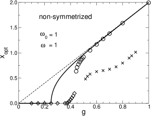
Figure 1: The plot of $x_{\rm opt}(g)$ for $\omega_{0}=\omega=1$, calculated with the non-symmetrized trial function (7). The solid curve is the variational ground state energy $E_{0}^{(1)}$, the dashed line is the large $g$-asymptotic. The CSM estimate $E_{0}^{(6)}$ has three blind arms denoted by symbols $\bigcirc$, $\diamondsuit$ and $\times$.

First we present the results for the non-symmetrized trial function $|\psi(x,y)\rangle$ (7). For any $\{\omega_{0},\omega,g\}$, the variational $E_{0}^{(1)}$ possesses just one minimum at $\{x_{\rm opt},y_{\rm opt}\}$ lying in the interval (10). Each of the functions $x_{\rm opt}(g)$ and $y_{\rm opt}(g)$ is continuous. The plot of $x_{\rm opt}(g)$ is represented in Fig. 1 by the solid curve [the picture is similar for $y_{opt}(g)$]. For $16g^{2}\leq\omega_{0}\omega$, the solution of Eq. (16) giving the minimum of $E_{0}^{(1)}$ is trivial: $\{x_{\rm opt},y_{\rm opt}\}=\{0,0\}$. This is why the curve $x_{\rm opt}(g)$ lies on the $g$ axis up to $g=1/4$. If $g>1/4$, the solution becomes non-trivial and approaches the asymptotic $x_{\rm opt}=2g/\omega$ (dashed line) for large $g$. Although this curve is continuous, it is non-analytic at the point $g=1/4$. Going to $E_{0}^{(m)}$ with $m\geq 3$, the number of minimum solutions to Eq. (16) can be larger than one in certain intervals of $g$. The minima curves can break at some points (beyond which there are no minimum solutions) or split into several curves. None of them goes continuously from small to large values of $g$.

Nevertheless, the curves denoted by open diamonds and circles in Fig. 1 can be used for small-$g$ and large-$g$ cases, respectively, to obtain satisfactory results. For small $g$, the trivial minimum $\{0,0\}$ can be directly inserted into all expressions. The variational $E_{0}^{(1)}(0,0)=-\omega_{0}/2$ and

$$E_{0}^{(3)}(0,0)=-\frac{\omega_{0}}{2}-\frac{4g^{2}}{\omega+\omega_{0}}.$$ (17)

For $g\ll\omega_{0}$, this formula is consistent with the exact result with the relative error $|E_{0}^{(3)}(0,0)-E_{0}^{\rm exact}|/E_{0}^{\rm exact}$ of the order $10^{-5}$. The large-$g$ results, illustrated in the first window of Table 1, are even more precise. We present the variational result $E_{0}^{(1)}$, the CSM $E_{0}^{(6)}$ and the numerically exact result [2]. The values of $\{x_{\rm opt},y_{\rm opt}\}$ and $\{x_{\rm opt}^{(6)},y_{\rm opt}^{(6)}\}$ are very close to the asymptotic result $\{2g/\omega,-1\}$. For example, for $\omega_{0}=\omega=1$ and $g=5$, the minimum of $E_{0}^{(6)}$ is at $\{9.99997,-0.997364\}$. The formulas with symmetrized trial functions (see bellow) lead to the results with comparable accuracy in both small-$g$ and large-$g$ regions.

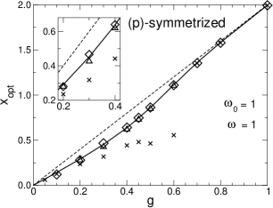
Figure 2: The plot of $x_{\rm opt}(g)$ for $\omega_{0}=\omega=1$, calculated with the $(p)$ symmetrized trial function (Optimized t-expansion method for the Rabi Hamiltonian). The solid curve corresponds to the variational $E_{0}^{(1,p)}$, the dashed line is the large $g$-asymptotic. The CMX estimate $E_{0}^{(5,p)}$: Optimized parameters closest to the solid curve are denoted by $\diamondsuit$, blind arms are denoted by $\triangle$ and $\times$.

Table 1. Estimates of the energies $E_{0}$ and $E_{1}$ for the Rabi Hamiltonian with $g=5$.

	$\omega_{0}=\omega=1$	$\omega_{0}=1,\omega=2$
$E_{0}^{(1)}$	-100.006250000	-50.001250000
$E_{0}^{(6)}$	-100.006265682	-50.001262703
$E_{0}^{\rm exact}$	-100.006265704	-50.001262758
$E_{1}^{(1,n)}$	-100.006250000	-50.001250000
$E_{1}^{(6,n)}$	-100.006265686	-50.001262703

The results for the ground state energy obtained with the $(p)$-symmetrized trial function $|\psi^{(p)}(x,y)\rangle$ (Optimized t-expansion method for the Rabi Hamiltonian) are presented in Fig. 2. The main advantage of the variational result $E_{0}^{(1,p)}$ in comparison with the non-symmetrized one is that the curve of unique minima, plotted as the solid curve, is not only continuous but also analytic for all $g$. In the considered higher orders $E_{0}^{(m,p)}$ $(3\leq m\leq 6)$ and for both CSM and CMX methods, there exists a unique counterpart of the variational curve of minima (represented by open diamonds) which is continuous and free of singular points in the whole interval of $g$ values; these are the accepted optimized minima. Similarly as for the non-symmetrized trial function, blind disconnected curves of minima appear (open triangles and crosses); we ignore them. Since some of minima are very close to the variational curve, the region of intermediate values of $g$ is magnified in the inset of Fig. 2.

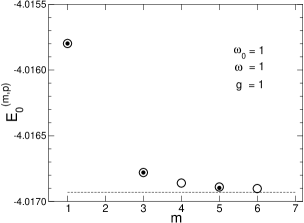
Figure 3: The ground-state energy $E_{0}^{(m,p)}$ for $\omega_{0}=\omega=g=1$, calculated with the $(p)$-symmetrized trial function: The CSM results $\bigcirc$ in $m=1,3,4,5,6$ orders, the CMX results $\bullet$ in $m=1,3,5$ orders. Dashed line is the numerically exact value [13].

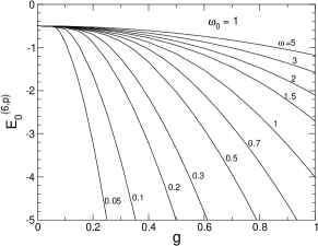
Figure 4: The CSM estimate of the ground state energy with the $(p)$ symmetrized trial function, $E_{0}^{(6,p)}$, for $\omega_{0}=1$, various discrete values of $\omega$ and the interaction parameters $g$ constrained to the interval $[0,1]$.

First we discuss the results for small-$g$. Bishop et al. [13] showed that for $g\ll\omega_{0}$ the coordinates of minima for the variational $E_{0}^{(1,p)}=\mu_{1}^{(p)}$ [see Eq. (15)] are, up to the term linear in $g$, given by

$$x_{\rm opt}\approx\frac{2g}{\sqrt{\omega(\omega_{0}+\omega)}},\quad y_{\rm opt}\approx-\frac{2g}{\omega_{0}+\omega}.$$ (18)

Inserting these values into $E_{0}^{(1,p)}$ and expanding in small $g$ up to the $g^{2}$ term we reproduce Eq. (17), derived from the non-symmetrized $E_{0}^{(3)}$. This coincidence confirms that the non-symmetrized trial function gives adequate results not only for large $g$, where the corresponding formulas effectively merge because the corresponding $x$ is large, but also in the region of small $g$.

For Rabi’s parameters $\omega_{0}=\omega=g=1$, a quick convergence of the results for the ground state energy $E_{0}^{(m,p)}$ to the exact value as $m$ increases is shown in Fig. 3. The CMX data are represented by full circles, the CSM data by open circles; note that the CMX and CSM results are very close to each other. The (numerically) exact value [13] is represented by the dashed line. The improvement of the variational $m=1$ result is remarkable already for $m=3$. As $m$ increases, the convergence of the data to the exact value is excellent.

Our procedure enabled us to calculate very quickly the CSM ground state energies $E_{0}^{(6,p)}$ for various sets of the Rabi Hamiltonian parameters, see Fig. 4. Without any loss of generality we set $\omega_{0}=1$. Each curve is labeled by the boson energy $0.05\leq\omega\leq 5$. The interaction parameter $g$ is constrained to $0\leq g\leq 1$. All values are correct within the resolution of the plots. The worst relative error of the order $10^{-4}$ was achieved for medium values of $g$.

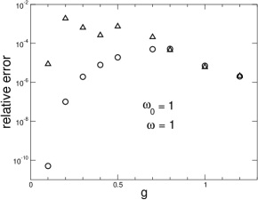
Figure 5: The relative error of the CSM estimates of the ground state energy $E_{0}^{(6,p)}$ [$(p)$ symmetrized trial function, open circles] and the first excited energy $E_{1}^{(6,n)}$ [$(n)$ symmetrized trial function, open triangles], for $\omega_{0}=\omega_{1}=1$ and an interval of $g$-values.

To document an extraordinary accuracy of the obtained results, in Fig. 5 we present the relative error of the CSM estimates of the ground state energy $E_{0}^{(6,p)}$ [$(p)$ symmetrized trial function, open circles] and of the first excited energy $E_{1}^{(6,n)}$ [$(n)$ symmetrized trial function, open triangles] for $\omega_{0}=\omega_{1}=1$ and an interval of $g$-values. Within the whole parameter space of the Rabi Hamiltonian, the relative error is smaller than $10^{-4}$ for $E_{0}$ and smaller than $10^{-2}$ for $E_{1}$. Like for example, our CSM results for the ground state energy $E_{0}^{(6,p)}$ are $-0.69761396$ for $g=0.3$ and $-0.87854267$ for $g=0.4$, the (numerically) exact values $E_{0}^{\rm exact}$ are $-0.69761529$ for $g=0.3$ and $-0.87854932$ for $g=0.4$ [16]. The relative errors are $1.9\times 10^{-6}$ and $7.8\times 10^{-6}$, respectively. As concerns the first excited energy, Bishop et al. [13] reported the largest relative error (almost $0.4$) for the variational estimate $E_{1}^{(1,n)}$ at the interaction constant $g=0.2$. We see in Table 2 that this error goes down quickly in higher approximation orders.

Table 2. Estimates and relative errors of $E_{1}$ for $\omega_{0}=\omega=1$ and $g=0.2$. aaaaaaaaaaaaaaaaa Estimate Rel. error  $E_{1}^{(1,n)}$ var. 0.00324806 0.39  $E_{1}^{(5,n)}$ CMX 0.00233753 0.000335  $E_{1}^{(6,n)}$ CSM 0.00234135 0.00197  $E_{1}^{\rm exact}$ 0.00233675 0

Conclusion: In conclusion, it turns out that the optimization of low orders of the $t$-expansion for the Rabi Hamiltonian improves remarkably the precision of the variational ground state estimates. In the whole parameter range of Rabi model, with the symmetrized trial function the relative error is smaller than $10^{-4}$ ($0.01$%). The accuracy of the $t$-expansion method is not ensured if the trial function is not properly chosen, as was seen in the case of non-symmetrized trial function and medium values of the interaction constant $g$.

References

- [1] V. Fessatidis, J. D. Mancini and S. P. Bowen Phys. Lett. A 297 (2002) 100.
- [2] P. Amore, F. M. Fernández and M. Rodriguez, arXiv:1010.5773v1 [quant ph].
- [3] D. Horn and M. Weinstein, Phys. Rev. D 30 (1986) 1256.
- [4] J. Cioslowski, Phys. Rev. Lett. 58 (1987) 83.
- [5] C. Stubbins, Phys. Rev. D 38, (1988) 1942.
- [6] L. Šamaj, P. Kalinay, P. Markoš and I. Travěnec, J. Phys. A 30 (1997) 1471.
- [7] J. D. Mancini, V. Fessatidis, R. K. Murawski and S. P. Bowen, Phys. Rev. B 72 (2005) 214405.
- [8] V. Fessatidis, J. D. Mancini, R. K. Murawski, S. P. Bowen and W. J. Massano, Phys. Lett. A 303 (2002) 72.
- [9] V. Fessatidis, J. D. Mancini, S. P. Bowen and W. J. Massano, Int. J. Quantum Chem. 6 (2005) 792.
- [10] V. Fessatidis, J. D. Mancini and S. P. Bowen Phys. Lett. A 372 (2008) 1155.
- [11] M. Kolesík and L. Šamaj, Phys. Lett. A 177 (1993) 87.
- [12] I. I. Rabi, Phys. Rev. 51 (1937) 652.
- [13] R. F. Bishop, N. J. Davidson, R. M. Quick and D. M. van der Walt, Phys. Lett. A 254 (1999) 215.
- [14] G. Qin, K.-L. Wang, T.-Z. Li, R.-S. Han and M. Feng, Phys. Lett. A 239 (1998) 272.
- [15] V. Fessatidis, J. D. Mancini, R. K. Murawski and S. P. Bowen, Phys. Lett. A 349 (2006) 320.
- [16] P. Amore, private communication.