∎
1010institutetext: A. Cavallo 1111institutetext: Dipartimento di Fisica, Università degli Studi di Salerno, via Ponte don Melillo, I-84084 Fisciano, Italy 1212institutetext: H. Xu 1313institutetext: LPMD, ICPM, Université Paul Verlaine Metz, 1 bd Arago, 57078 Metz Cedex 03, France 1414institutetext: S. Obukhov 1515institutetext: Department of Physics, University of Florida, Gainesville FL 32611, USA
Scale-free static and dynamical correlations in melts of monodisperse and Flory-distributed homopolymers
Abstract
It has been assumed untill very recently that all long-range correlations are screened in three-dimensional melts of linear homopolymers on distances beyond the correlation length characterizing the decay of the density fluctuations. Summarizing simulation results obtained by means of a variant of the bond-fluctuation model with finite monomer excluded volume interactions and topology violating local and global Monte Carlo moves, we show that due to an interplay of the chain connectivity and the incompressibility constraint, both static and dynamical correlations arise on distances . These correlations are scale-free and, surprisingly, do not depend explicitly on the compressibility of the solution. Both monodisperse and (essentially) Flory-distributed equilibrium polymers are considered.
Keywords:
Polymer melts Monte Carlo simulations Time-dependent propertiespacs:
61.25.H- 05.10.Ln 82.35.Lr 61.20.Lc1 Introduction
1.1 General context
Solutions and melts of macromolecular polymer chains are disordered condensed-matter systems ChaikinBook of great complexity and richness of both their physical and chemical properties FloryBook ; DegennesBook ; DoiEdwardsBook ; BenoitBook ; DescloizBook ; SchaferBook ; RubinsteinBook . Being of great industrial importance and playing a central role in biology and biophysics RubinsteinBook ; OozawaBook , they represent one relatively well-understood fundamental example of the vast realm of so-called “soft matter” systems WittenPincusBook comprising also, e.g., colloids DhontBook , liquid crystals ChaikinBook and self-assembled surfactant systems WittenPincusBook .111A soft matter system may be defined as a fluid in which large groups of the elementary molecules have been permanently or transiently connected together, e.g. by reversibly bridging oil droplets in water by telechelic polymers or similar systems of autoassociating polymers ANS95 ; ANS00 ; ANS01 , so that the permutation freedom of the liquid state is lost for the time window probed experimentally WittenPincusBook . The thermal fluctuations which dominate the liquid state must thus coexist with constraints reminiscent of the solid state. Reflecting this solid state characteristics the dynamic shear-modulus thus often remains finite up to macroscopic times and the associated shear viscosity may become huge. Most soft matter systems behave as liquids for very long times, i.e. for and remains finite. The notion “polymer” is not limited to the hydrocarbon macromolecules of organic polymer chemistry à la H. Staudinger or W.H. Carothers PolymerPioneersBook ; InventingPolymerBook but refers also to biopolymers such as DNA or corn starch WittenPincusBook ; RubinsteinBook and various self-assembled essentially linear chain-like supramolecular structures such as, e.g., actin filaments OozawaBook or wormlike giant micelles formed by some surfactants WittenPincusBook ; CC90 .
Obviously, dense polymeric systems are quite complicated, but since their large scale properties are dominated by the interactions of many polymers, each of these interactions should only have a small (both static and dynamical) effect. A sound theoretical starting point is thus to add up these small effects independently and to correct then self-consistently for the deviations due to correlations between the interactions DoiEdwardsBook .222As seen in Sec. 2, it is, e.g., necessary to “renormalize” DegennesBook the local bond length to the “effective bond length” DoiEdwardsBook or the second virial coefficient of the monomers to the “effective bulk modulus” ANS05a to take into account the coupling of a reference chain to the bath. Obviously, the number of chains a reference chain interacts with, and thus the success of such a mean-field approach, depends an the spatial dimension of the problem considered. Let be the number of monomeric repeat units per polymer chain (with ), their typical size, their self-density (also called “overlap density”) and their inverse fractal dimension MandelbrotBook . Assuming the monomer number density to be -independent, a mean-field theoretical approach may be hoped to be successful if DegennesBook
| (1) |
For to leading order Gaussian chains () this implies that typically chains interact in . Hence, dense three-dimensional (3D) polymeric liquids should be much easier to understand than normal liquids, say benzene and let alone water, where each molecule has only a few, say ten, directly interacting neighbors Israela .
1.2 Coarse-grained lattice models for polymer melts
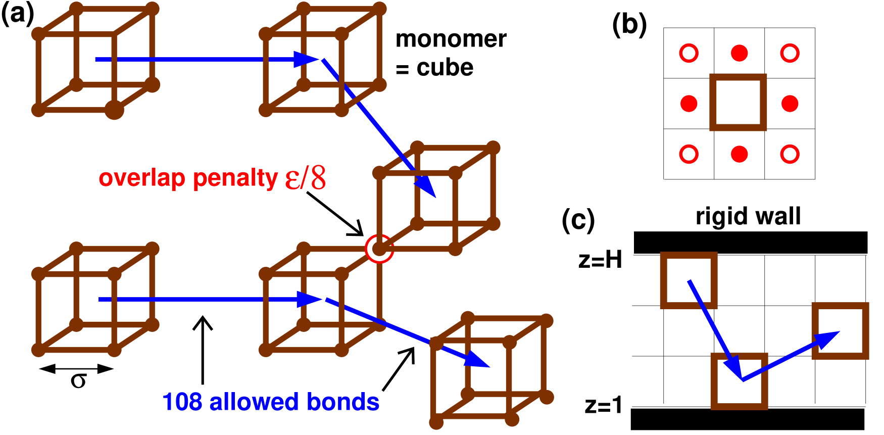
Focusing on the generic statistical properties of flexible and neutral homopolymer melts in ,333Although we focus on 3D bulks the general -dependence is often indicated since this may help to clarify the intrinsic structure of the relations. The reader is invited to replace by . For similar reasons we often make explicit the inverse fractal dimension . It should be replaced by its value . one of the simplest idealizations consists, as illustrated in Fig. 1, in replacing the intricate chemical chain structure by self-avoiding walks on a periodic lattice FloryBook ; DegennesBook ; VanderzandeBook .

Let us assume canonical ensemble statistics AllenTildesleyBook ; ThijssenBook ; FrenkelSmitBook ; BinderHerrmannBook ; LandauBinderBook ; KrauthBook where the total monomer number , the volume of the -dimensional simulation box and the temperature are imposed. (Boltzmann’s constant is set to unity throughout the paper.) A bond vector connecting the monomers and is not necessarily restricted to a step of length (with being the lattice constant) to the next-nearest lattice site. As in the well-known bond-fluctuation model (BFM) BFM ; BWM04 ; BFMreview05 presented in detail in Sec. 3, one may in general take bonds from a suitably chosen set of allowed lattice vectors to achieve a better representation of the continuum space symmetries of real polymers ChaikinBook ; Wang09b . We focus on systems of high monomer number density . In principle, although not in practice as seen below, one could sample the configuration space of such a lattice polymer melt using a Monte Carlo (MC) algorithm LandauBinderBook ; KrauthBook with local hopping move attempts to the next-nearest neighbor sites on the lattice, as shown for the monomer in panel (a). The specific local MC move illustrated is an example for the more general local and global rearrangements of the monomers KrauthBook ; BWM04 ; Kron65 ; Wall75 ; dePablo94 ; pakula02 ; Theodorou02 ; dePablo03 (respecting the set of allowed bond vectors) one may implement as discussed in Sec. 3.3. Due to their simplicity and computational efficiency, such coarse-grained lattice models have become valuable tools for the numerical verification of theoretical concepts and predictions FloryBook ; VanderzandeBook ; BFMreview05 , especially focusing on scaling properties in terms of the chain length or the arc-length of subchains DegennesBook .
1.3 Flory’s ideality hypothesis for polymer melts
One of the most central concepts of polymer physics is that in a polymer melt all long-range static and dynamical correlations are generally assumed to be negligible beyond the screening length (defined properly in Sec. 2.3 and tested numerically in Sec. 4.4) characterizing the decay of the density fluctuations DoiEdwardsBook . The polymer chains are thus expected to adopt random-walk statistics as already stated by Flory in the 1940th FloryBook ; Flory45 ; Flory49 and worked out more systematically in terms of a perturbation theory by Edwards two decades later DoiEdwardsBook ; Edwards65 ; Edwards66 ; Edwards75 ; Edwards82 . The (normalized) probability distribution of the end-to-end distance of a subchain of a sufficiently large arc-length should thus be a Gaussian,
| (2) |
for and with being the “effective bond length” and the arc-length spanning the correlation length . Note that in general the effective bond length differs for various reasons from the root-mean-squared bond length between monomers and ultimately must be fitted as will be shown in Sec. 5.3. One immediate consequence of Eq. (2) is of course that the second moment of must increase linearly,
| (3) |
and the same holds for the mean-squared total chain end-to-end distance with , i.e. for the inverse fractal dimension. Since the bond-bond correlation function measures the curvature of the mean-squared subchain size ,
| (4) |
it follows from Eq. (3) that for .444This lack of memory of the bond orientations may be taken as the defining statement of Flory’s ideality hypothesis. Using the central limit theorem DhontBook one immediately gets back to Eq. (2). This suggests to test for possible deviations from by computing directly the bond-bond correlation function as we shall do in Sec. 5.4. That Eq. (4) holds follows from the general relation for displacement correlations Eq. (173) demonstrated in Appendix A.555It is also common to define the bond-bond (or angular) correlation function as the first Legendre polynomial using the normalized tangent vector . The difference between and is irrelevant from the scaling point of view and negligible quantitatively for all computational models we have studied. Higher order angular correlations may be described in terms of general Legendre polynomials abramowitz sampled as a function of the arc-length between the bond pair or their spatial distance . The polynomials may be used to characterize the interchain angular correlations, a question out of the scope of the present study.
1.4 Rouse model hypothesis for polymer melts
Based on Flory’s ideality hypothesis for the chain conformations, the celebrated reptation model suggested by Edwards and de Gennes DegennesBook ; DoiEdwardsBook provides a widely accepted theoretical description for the dynamical properties of entangled polymer melts explaining qualitatively the observed increase of the melt viscosity with respect to the chain length and other related observables Lodge90 . The central idea is that chains cannot cross each other and must due to this topological constraint “reptate” along an effective “primative path” set by their own contour.666In its original formulation the reptation model is a single chain mean-field theory, the constraints due to other chains being accounted for by the effective topological tube DoiEdwardsBook . Due to density fluctuations generated by the motion of the chains and the finite compressibility of the elastic mesh, different chains must be coupled, however. As suggested by A.N. Semenov et al. ANS97 ; ANS98 , the relaxational dynamics of long reptating chains ( in ) is ultimately “activated”, i.e. the longest relaxation time and the viscosity increase exponentially with chain length and not as simple power laws Deutsch85 ; MWBBL03 . Using local topology conserving MC moves various authors have thus attempted in the past to verify the reptation predictions by lattice MC models as the one sketched in Fig. 1 Paul91a ; Paul91b ; WPB92 ; WPB94 ; Shaffer94 ; Shaffer95 ; KBMB01 ; HT03 . Similar tests have also been performed by means of molecular dynamics (MD) FrenkelSmitBook , Brownian dynamics (BD) AllenTildesleyBook and MC simulations of various off-lattice bead-spring models KG86 ; KG90 ; LAMMPS ; Briels01 ; Briels02 ; EveraersScience ; MKCWB07 ; Wang09a .777The computational activities have focused recently on the latter off-lattice models, one essential advantage being that the experimentally relevant shear-stress correlation function can be computed directly without using additional input from theory.
We remind that reptational motion along the primative path is assumed to be the dominant relaxational process only for chains much longer than the (postulated) entanglement length and for times larger than the entanglement time DegennesBook . In the opposite limit the dynamics is thought to be described by the Rouse model proposed in the 1950th, i.e. by a simple (position) Langevin equation for a single chain with all interactions from the bath being dumped into a friction term and random uncorrelated forces DegennesBook . Thus the reptation model “sits on top” of the Rouse model and should the latter model prove not to be sufficient this must be relevant for long chains in the entangled regime.888As a consequence of the “hydrodynamic screening hypothesis” for dense polymer solutions DoiEdwardsBook , all Zimm-like long-range correlations are generally regarded to be negligible beyond the static screening length Duenweg93 ; Duenweg01 ; Spenley00 . The monomer momentum is not lost, of course, but transmitted to the bath and for large times and distances the melt is still described by the Navier-Stokes equation ChaikinBook . Although these hydrodynamic effects are beyond the scope of this paper focusing on lattice MC simulations, a short hint on scale-free corrections to the hydrodynamic screening hypothesis is given at the end of Sec. 7.2.
Interestingly, it is relatively easy to construct for the lattice models sketched in Fig. 1 local monomer moves switching off the topological constraints without changing the excluded volume and other interactions and conserving thus all static properties. This has allowed to demonstrate that topological constraints are paramount for the relaxation process Shaffer94 ; Shaffer95 . Since the local MC hopping attempts correspond to the random white forces of the Rouse model and since all other long-range correlations of the bath are supposed to be negligible beyond , one generally assumes that such a topology non-conserving lattice model should be described by the Rouse model for chain lengths . Since the forces acting on the chain center-of-mass (CM) are uncorrelated, the probability distribution of the CM displacements must be a Gaussian just as Eq. (2) with the CM displacement replacing , the time replacing the arc-length and replacing . The self-diffusion coefficient and the longest Rouse relaxation time of chains of length should scale as DoiEdwardsBook
| (5) |
with being a convenient local monomer mobility defined properly in Sec. 6.3 Paul91b . In analogy to Eq. (3), may be obtained by fitting the mean-square displacement (MSD) of the chain CM
| (6) |
The chain relaxation time corresponds to the motion of the CM over the typical chain size and may be defined by setting Paul91b . Note that Eq. (6) should hold for all times (taken apart very short times corresponding to displacements of order of or the lattice constant ) and not only for as for reptating chains. In analogy to Eq. (4) one may characterize the CM displacements by a four-point correlation function in time, the “velocity correlation function” (VCF)
| (7) |
which measures directly the curvature of with respect to time with being the CM displacement for a time window . Since in a MC algorithm there is no velocity in the sense of an Euler-Lagrange equation, “velocity” refers to the displacement per time increment . As shown in Appendix A, Eq. (7) states that becomes independent of for . Since Eq. (6) implies that must vanish for all times, this begs for a direct numerical test as will be discussed in Sec. 6. Interestingly, the above statements do not only hold for the displacement field of the total chain CM but also for the displacements of the CM of arbitrary subchains of arc-length for times with being the Rouse relaxation time of the subchain.999For times a subchain feels the connectivity with the rest of the chain and must follow the typical monomers motion for . We can thus state more generally that according to the Rouse model one expects
| (8) |
with being the VCF associated to the subchain CM displacements .
1.5 Aim of this study and key results
Summarizing recent theoretical and numerical work made by the Strasbourg polymer theory group but also by other authors SchaferBook ; Obukhov81 ; Schweizer91 ; MM00 ; Wang02 ; Auhl03 ; Rubinstein08 ; Morse09 ; Morse09b ; Paul98 ; Smith00 ; PaulGlenn , we address and question in this review the validity of the general screening assumption for dense polymer solutions and melts both concerning Flory’s ideality hypothesis for the chain conformations WMBJOMMS04 ; WBCHCKM07 ; WBJSOMB07 ; BJSOBW07 ; WBM07 ; MWK08 ; WCK09 ; WJO10 ; WJC10 ; ANS10a and the Rouse model assumption for the dynamics of systems with irrelevant or switched off topology WPC11 ; papFarago ; ANS11a ; ANS11b . We argue that due to the overall incompressibility of the polymer melt both the static and the dynamical fluctuations of chains and subchains are coupled on scales beyond the screening length . In dimensions this leads to weak but measurable scale-free deviations which do not depend explicitly on the (low but finite) isothermal compressibility of the solution.
The static correlations are made manifest by the finding WMBJOMMS04 ; WBM07 ; MWK08 ; WCK09 that the intrachain bond-bond correlation does not vanish as implied by Flory’s hypothesis, but rather decays analytically in dimensions as
| (9) |
the amplitude being given by the dimensionless stiffness coefficient DoiEdwardsBook and the so-called “swelling coefficient” WBM07 . Due to Eq. (4) this is consistent with a typical subchain size
| (10) |
i.e. approaches the asymptotic limit monotonously from below and the chain conformations are thus weakly swollen as shown in Sec. 5.3.2. Note that generalizing Eq. (9) as demonstrated in Appendix B.4 the bond-bond correlation function is predicted to decay in (effectively) dimensions as ANS03 ; CMWJB05 ; LFM11 ; thinfilmdyn
| (11) |
for with being the -dimensional monomer density.101010For the range of validity of Eq. (11) is further restricted as discussed in Sec. 7.2.1.
At variance to Eq. (8) the displacement correlation functions and of chains and subchains are observed not to vanish. Instead an algebraic long-time power-law tail
| (12) |
is found in for all and WPC11 . Due to Eq. (7) this finding implies for that the CM MSD of chains takes an additional algebraic contribution which dominates for short times such that
| (13) |
in qualitative agreement with the anomalous power-law exponent obtained in various numerical Paul91b ; Shaffer95 ; KBMB01 ; HT03 ; KG90 ; Briels01 ; Briels02 ; Skolnick87 ; Guenza02 ; Theodorou03 ; Theodorou07 and experimental studies Paul98 ; Smith00 ; PaulGlenn . Our theoretical and numerical result, Eq. (12), may thus help to clarify a long-lasting debate.111111We emphasize that Eq. (11) and Eq. (12) are both scale-free and do not depend explicitly on the compressibility of the solution. Interestingly, both key findings depend on the subchain length considered and not on the total chain size as long as .
1.6 Outline
We begin this review by summarizing in Sec. 2 a few well-known theoretical concepts from polymer theory and outline the perturbation calculations which lead, e.g., to Eq. (9).
Since the predicted deviations Eq. (9) and Eq. (12) are rather small in dimensions, the key challenge from the computational side is to obtain high precision data for well-equilibrated polymer melts containing sufficiently long chains to avoid chain end effects. This review focuses on numerical results obtained by means of the BFM algorithm with finite excluded volume interactions WCK09 and topology violating local and global Monte Carlo moves WBM07 as described in Sec. 3.121212To check for caveats due to our lattice model we have verified our results by MD simulation of a standard bead-spring model with and without topological constraints WMBJOMMS04 ; WBJSOMB07 ; WBM07 ; MWK08 ; papFarago ; ANS11a ; ANS11b . In order not to overburden the present summary, this story must be told elsewhere. Our numerical data for monodisperse melts are crosschecked WBCHCKM07 ; BJSOBW07 ; WJO10 ; WJC10 using systems of annealed size-distribution, so-called “equilibrium polymers” (EP) CC90 ; Scott65 ; Wheeler80 ; Faivre86 ; Milchev95 ; WMC98a ; WMC98b ; Milchev00 ; HXCWR06 ; Kroeger96 ; Padding04 , where chains break and recombine constantly and for this reason the sampling becomes much faster than for monodisperse quenched chains (Sec. 3.5).
Static properties are discussed in Sec. 4 and Sec. 5. In the first section we investigate some thermodynamic properties of dense BFM solutions such as the chemical potential in EP systems in Sec. 4.6 WJC10 . We verify in Sec. 4.4 the range of validity of the (static) “Random Phase Approximation” (RPA) DoiEdwardsBook describing the coupling of the total density fluctuations, encoded by the total structure factor at wavevector , with the degrees of freedom of tagged chains, encoded by the intrachain coherent single chain form factor BenoitBook . Section 5 contains the central part of our work related to conformational intrachain properties where we demonstrate Eq. (9). The deviations from Flory’s ideality hypothesis are also of experimental relevance, as shown in Sec. 5.7, since the measured form factor should differ from the corresponding Gaussian chain form factor as WBJSOMB07 ; BJSOBW07
| (14) |
Our work on dynamical correlations in Rouse-like systems without topological constraints WPC11 ; papFarago is summarized in Sec. 6. A simple perturbation theory argument leading to Eq. (12) will be given in Sec. 6.6. This argument uses the “dynamical Random Phase Approximation” (dRPA) ANS86 ; ANS97b ; papFarago describing the coupling of the degrees of freedom of the bath (encoded by the dynamical structure factor ) to the degrees of freedom of a tagged test chain (encoded by the dynamical form factor ). We shall verify explicitly this important relation.
We conclude the paper in Sec. 7 where we comment on related computational work focusing on dimensionality effects (Sec. 7.2.1) ANS03 ; CMWJB05 ; Brochard79 ; LFM11 , collective interchain correlations (Sec. 7.2.2) ANS05a ; ANS05b and long-range viscoelastic hydrodynamic interactions (Sec. 7.2.3) ANS11a ; ANS11b . Several theoretical issues are relegated to the Appendix.
2 Some theoretical considerations
2.1 Introduction
Let us go back to the simple generic lattice model sketched in Fig. 1. Simplifying further, we begin in Sec. 2.2 by switching off all short- and long-range interactions between chains and monomers, the only remaining interaction being the connectivity of the monomers along the chain contours. Translational invariance along these contours is assumed. No particular meaning is attached to the orientation of the monomer index .131313This implies symmetry with respect to the monomer index which can be read as a time variable as seen in Appendix A. Due to this reversibility the bond-bond correlation function can be expressed in terms of the non-Gaussian “colored forces” vanKampenBook acting on the monomers, Eq. (176). To make this toy model more interesting let us on the other side introduce two additional features: local chain rigidity (Sec. 2.2.1) and polydispersity (Sec. 2.2.2). Reminding some standard properties DegennesBook ; DoiEdwardsBook ; BenoitBook ; SchaferBook ; RubinsteinBook we will then introduce for later reference the intrachain single chain form factor (Sec. 2.2.4) and the total monomer structure factor (Sec. 2.2.4). Since the chains do not interact we can consider each chain independently. The interaction between chains and monomers will be switched on again in Sec. 2.3 by means of a Lagrange multiplier limiting the density fluctuations (Sec. 2.3.2). Note that assuming Flory’s ideality hypothesis most intrachain properties discussed in Sec. 2.2 should also hold rigorously in incompressible melts with the effective bond length being the only fit parameter. The effective entropic correlation hole forces for chains and subchains arising due to the incompressibility constraint are introduced in Sec. 2.3.4. The generic scaling of the deviations from Flory’s ideality hypothesis is motivated in Sec. 2.3.6 before we turn to the systematic perturbation calculation in Sec. 2.4. Following Muthukumar and Edwards Edwards82 we argue that the reference length of the Gaussian reference chain of the calculation (Sec. B.2) should be renormalized (Sec. 2.4.5). The bond-bond correlation function for asymptotically long chains is presented in Sec. 2.4.6 before we turn finally in Sec. 2.4.7 to finite chain size effects.
2.2 Connectivity constraint
2.2.1 Local rigidity
Keeping only the chain connectivity we switch off all other monomer and chain interactions. Let us apply a local stiffness energy proportional to the cosine of the bond angle , , with being the unit tangent vector. The stiffness energy is assumed to be not too large to avoid lattice artifacts WPB92 . Due to the multiplicative loss of any information transferred recursively along the chain contour the bond-bond correlation function must decay exponentially with arc-length FloryBook ,
| (15) |
with being the curvilinear persistence length, i.e. for . Using Eq. (4) it follows of course that for subchains of arc-length . Assuming Eq. (15) this implies for the effective bond length since more generally it is known that BWM04
| (16) |
The latter relation is consistent with the more common definition DoiEdwardsBook 141414Definitions based on such “Einstein relations” ChandlerBook are generally more robust numerically.
| (17) |
using the total chain mean-squared end-to-end distance DoiEdwardsBook . We have introduced here a convenient monomeric length allowing to simplify prefactors depending in a spurious manner on the spatial dimension and have reminded the dimensionless stiffness parameter .
We note that a good approximation for a “freely rotating chain” with local stiffness potential is given by DoiEdwardsBook
| (18) |
which has been shown to be useful even for lattice models with discrete bond angles WPB92 . In summary, a local stiffness energy does not change the scaling of the chain and subchain size with, respectively, or , but merely increases its amplitude. Note that a weak local chain stiffness with would be generated by disallowing chains to return after, say, two steps to the same lattice site (so-called “non-reversal random walks” BinderHerrmannBook ) and similar local constraints. Since these are the only local stiffness contributions which may occur in the presented numerical work these small rigidity effects can be safely disregarded below.151515The only case where the small local chain rigidity qualitatively matters is presented in Sec. 5.4.2 for the bond-bond correlation function for large distances between bonds WJO10 .
2.2.2 Polydispersity
Let us relax the monodispersity constraint made above and assume a general (normalized) probability distribution for chains of length . We suppose that the mean chain length is arbitrarily large and that all moments of the distribution exist. For subchain properties everything remains as before. Let us call the typical mean-squared chain size of chains of length . Since one averages experimentally over chains of different length this total average depends now on the moment of the distribution which is probed,
| (19) |
with being the -averaged chain length. Since for experimentally reasonable distributions , we have normally with numerical coefficients due to the moment taken. For the properties considered by us, it is the so-called “-average” for which matters most. The -average is for instance probed by sedimentation in an analytical ultracentrifuge or in neutron scattering measurements of the intramolecular form factor as further discussed in Sec. 2.2.4 BenoitBook . Note that all standard definitions and formulas DegennesBook ; DoiEdwardsBook are recovered for a monodisperse length distribution .
For the important case of Flory-distributed polymers with
| (20) |
we have and thus . Such a Flory distribution is expected for systems of EP with an annealed length distribution where a constant finite scission energy has to be paid for the scission of each bond as described in Sec. 3.5. This can be seen by minimizing the Flory-Huggins free energy functional OozawaBook ; CC90 ; WMC98b
| (21) |
with respect to the density of chains of length . The first term on the right is the usual translational entropy. The second term entails a Lagrange multiplier which fixes the total monomer density
| (22) |
All contributions to the chemical potential of the chain which are linear in can be absorbed within this Lagrange multiplier. The scission energy characterizes the imposed enthalpic free energy cost for breaking a chain bond. The last term encodes the remaining non-linear contribution to the chemical potential which has to be paid for creating two new chain ends.161616As shown in Sec. 4.6 and Sec. B.6, the free energy contribution may depend in general on the chain length DescloizBook ; SchaferBook ; WMC98a . For non-interacting random walks on the lattice this contribution is just a (model depending) constant entropic factor which renormalizes the imposed scission energy to an -independent effective scission free energy HXCWR06 . The minimization of Eq. (21) under the density constraint, Eq. (22), yields Eq. (20) with a mean chain length
| (23) |
as the reader will readily verify.
2.2.3 Segmental size-distribution
Due to the translational invariance in space and along the chain contours most perturbation calculations outlined below BJSOBW07 ; WBM07 ; WJO10 ; WJC10 are more readily performed in reciprocal space. The Fourier transform of a function is denoted and we write for the Laplace transform of a function with being the Laplace variable conjugated to the arc-length . We have introduced in Sec. 1.3 the probability distribution of the end-to-end distance of a subchain of arc-length between the monomers and of a chain. The Fourier transform of this two-point intramolecular correlation function is thus in general with the average being taken over all possible subchain vectors . For (infinite) Gaussian chains this becomes DoiEdwardsBook
| (24) |
The index has been introduced for the general case where may differ from the Gaussian propagator used in our perturbation calculations. Moments of the distribution are readily obtained from derivatives of taken at as recalled in Appendix B.1 vanKampenBook . It follows for instance for the -th moment of the distribution that
| (25) |
for Gaussian chains. We have thus
| (26) |
A very closely related characterization of is given by the standard non-Gaussianity parameter
| (27) |
which for Gaussian chains is identical to . As further discussed in Sec. 5.5, has computationally the advantage that the effective bond length must not be known a priori. Obviously, the general distribution is fully determined by either the dimensionless moments or vanKampenBook .
In Fourier-Laplace space the Gaussian propagator reads
| (28) |
If one needs to average over all bond pairs at a given distance irrespective of their curvilinear distance , and one has thus to sum over all possible as in Sec. B.5, this corresponds (for arbitrarily large chains) to setting for the corresponding Laplace variable. The summed up Gaussian propagator for infinite chains is thus . For Flory-distributed Gaussian chains of finite mean chain length we have more generally a summed up Gaussian propagator
| (29) |
Inverse Fourier transformation yields in the density
| (30) |
around a tagged reference monomer of all the monomers belonging to the same chain. Obviously, for one recovers the well-known density
| (31) |
for infinite objects of inverse fractal dimension DegennesBook ; WittenPincusBook .171717The reader may verify the indicated scaling by direct integration of Eq. (2) with respect to for monodisperse chains with . This power-law dependence of the local density means that our random-walk polymer is a fractal set in the sense of Mandelbrot MandelbrotBook , i.e. the average mass (number of monomers) within a distance of an arbitrary point of the set varies as a power of . The -dependence of the local density reflects a type of spatial order that is not connected to translation or rotation symmetries but to the “dilation transformation” to a magnified system DegennesBook . A structureless, uniform material looks the same when magnified, provided the magnification is too weak to see the molecular constituents (“lower cutoff”). The scaling exponent characterizes the dilation symmetry in the same way that linear momentum characterizes translational symmetry and angular momentum characterizes rotational symmetry WittenPincusBook .
2.2.4 Intramolecular coherent form factor
The two-point correlation function may be probed experimentally through the intramolecular form factor which for monodisperse chains is defined by DoiEdwardsBook
| (32) | |||||
| (33) |
with and . The second representation being an operation linear in has obvious computational advantages for large chain lengths. In principle, the characteristic polymer size may be obtained experimentally from in the Guinier regime for small BenoitBook . Expanding Eq. (32) yields with being the gyration radius defined as
| (34) |
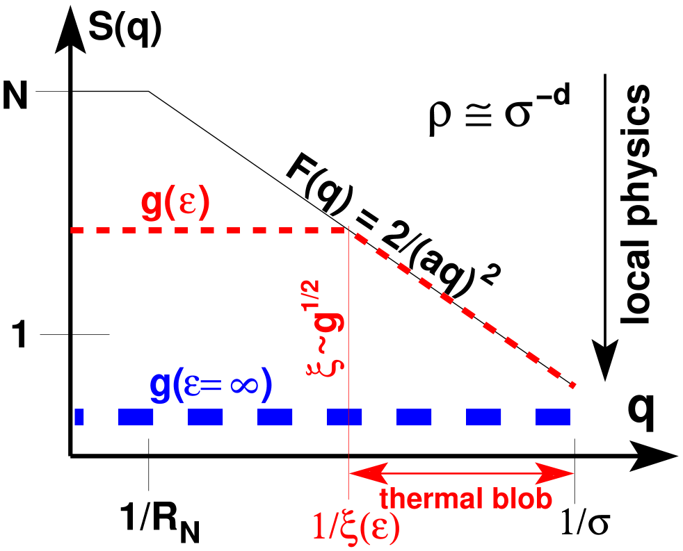
For chains following Gaussian statistics (as our lattice chains with switched off interactions) where , it follows by integration of Eq. (34) that . For large wavevectors where the internal fractal chain structure is probed, the form factor decays as
| (35) |
as sketched by the thin line in Fig. 2.181818The power-law scaling is obtained directly by Fourier transformation of Eq. (31) which yields . This scaling only holds if the fractal object is “open”, i.e. , and the scattering intensity is not dominated by the Porod scattering at the (possibly fractal) “surface” of a compact object BenoitBook ; MSZ11 . The latter Porod scattering becomes relevant, e.g., for self-avoiding polymers in strictly dimensions MKA09 ; MWK10 and for non-olympic and un-knotted rings in or thin films of finite width () MWC00 ; Vettorel09 ; MSZ11 . In both cases the polymers adopt compact configurations, , with a fractal surface of well-defined fractal surface exponent . The form factor thus decays as MSZ11 . More generally, the form factor of monodisperse Gaussian chains is given by with and the Debye function
| (36) |
For convenience of calculation, the Debye function is often replaced by the Padé approximation
| (37) |
where the last step holds for .
For a general mass distribution the form factor is defined as BenoitBook ; DescloizBook ; BJSOBW07
| (38) |
In practice, Eq. (38) corresponds to the computation of the averaged sum over contributions for each chain which one divides finally by the total number of labeled monomers BJSOBW07 . In the small- regime one obtains again a Guinier relation
| (39) |
where stands now for the -averaged gyration radius DescloizBook where the moment is taken over the standard radius of gyration , Eq. (34). Note that for Flory-distributed Gaussian chains we have and the form factor becomes BJSOBW07
| (40) |
Eq. (40) reduces to Eq. (35) for large wavevectors, as one expects, since in this limit must become independent of the length distribution . Note that Eq. (40) has the same form as the Padé approximation for monodisperse chains, Eq. (37).
2.2.5 Total monomer structure factor
For non-interacting chains the local monomer density can freely fluctuate being restricted only by the chain connectivity. The isothermal compressibility ChaikinBook is thus given by the osmotic contribution due to the density of chains, i.e. diverges linearly with the typical chain length . More generally, one may characterize the fluctuations of the total density in Fourier space by means of the total structure factor DoiEdwardsBook
| (41) | |||||
with being a wavevector commensurate with the simulation box191919If we use a cubic simulation box of linear dimension the smallest possible wavevector is . and the thermal average being performed over all configurations of the ensemble and all possible wavevectors of length . Since we have switched off all monomer interactions, monomers on different chains are uncorrelated and, hence,
| (42) |
as indicated for monodisperse chains by the thin line in Fig. 2. Due to the chain connectivity the fluctuations of chains (measured by ) and the fluctuations of monomers (measured by ) may differ for polydisperse non-interacting systems: While in the small- limit as seen from Eq. (39), we have for the compressibility.202020The dimensionless compressibility defined in Eq. (43) for asymptotically long chains does not depend on this ideal chain contribution. Care is needed, however, if is determined numerically from for polydisperse systems of finite by extrapolation in analogy to the monodisperse case discussed in Sec. 4.4.
2.3 Incompressibility constraint
2.3.1 Dimensionless compressibility
Obviously, dense polymer solutions and melts are essentially incompressible, i.e. , and the above assumption that the total density can freely fluctuate is not very realistic. It is useful to introduce here a central dimensionless thermodynamic property characterizing the degree of density fluctuations on large scales, the so-called “dimensionless compressibility” BJSOBW07 ; WBM07 ; WCK09
| (43) |
At standard experimental polymer melt conditions remains of course finite, say , but typically well below unity as indicated by the bold dashed line in Fig. 2 RubinsteinBook . Note that we have defined in the limit of asymptotically long chains to take off the trivial compressibility contribution due to the translational invariance of the chains mentioned above. For later reference we have also introduced in Eq. (43) the effective “bulk modulus” ANS05b . As indicated, the dimensionless compressibility can be determined directly in experiments or in a computer simulation from the low- limit of the total monomer structure factor . This point is further elaborated in Sec. 4.4.
2.3.2 Lagrange multiplier
Physically, the incompressibility of dense polymer systems arises of course due to the short-range repulsion of the monomers, i.e. it depends on non-universal physical and chemical properties. From the theoretical and computational point of view it is, however, inessential how the incompressibility at low wavevectors is imposed.212121If the goal is to map a computational model onto a real polymer melt aiming to understand macroscopic properties, the starting point should be, in our opinion, to match the mechanical and thermodynamic properties in the low- limit, e.g. the dimensionless compressibility , rather than to fiddle with on the monomer scale. This constraint could be achieved, at least in principle, by “simple sampling” LandauBinderBook of only those configurations respecting the chosen . In this sense it is thus the “throwing away” of configurations from the extended configuration ensemble containing all possible linear chain paths on the lattice which creates the repulsive forces between chains, subchains and monomers.222222The scale-free correlations described in this paper are thus akin to the effective “anti-Casimir forces” which arise in dense polymer melts due to the throwing away of configurations containing closed loops from an extended configuration ensemble with both linear chains and rings ANS05a ; ANS05b . Alternatively, one may design intricate local and global MC moves forcing the system through configuration space along a hyperplane of constant KrauthBook ; BWM04 .
A more general and computationally more natural route is to use an extended ensemble LandauBinderBook and to impose the incompressibility constraint through an external field with a Lagrange multiplier conjugated to the local monomer density fluctuations. As may be seen in more detail in Sec. 3.4 for a specific lattice model, this implies in practice that one has to pay an energy of order for the overlap of two monomers. While in the low- limit with the chains do not interact, i.e. for all , the incompressibility constraint holds for all wavevectors up to the monomeric scale () in the opposite limit . This is shown by the bold dashed line in Fig. 2.
2.3.3 Thermal blobs of size
The situation is slightly more complicated for intermediate overlap penalties with indicated by the thin dashed line. Since is now a well-defined characteristic chain length in curvilinear space along the chain contour, it corresponds to a characteristic scale in real space, the “screening length” of the density fluctuations defined as DoiEdwardsBook
| (44) |
where we use the effective bulk modulus following Eq. (43).232323From the scaling point of view a curvilinear length translates quite generally to a spatial distance and a wavevector according to with being the inverse fractal dimension. Generalizing Eq. (42) to systems with finite compressibility the total structure factor is predicted to follow the so-called (static) “Random Phase Approximation” (RPA) DegennesBook ; DoiEdwardsBook ,
| (45) | |||||
| (46) |
using Eq. (35) in the second step. The Ornstein-Zernike correlation equation DhontBook Eq. (46) justifies the above definition of the “screening length” , i.e. density fluctuations decay in exponentially as DoiEdwardsBook
| (47) |
We remind that sets the size of the “thermal blob” DegennesBook corresponding to a free energy due to the effective monomer interaction of order . If one considers short subchains of arc-length or small distances , the (sub)chains behave as if they were barely interacting, i.e. . If on the other side one focuses on the physical properties beyond the thermal blob scale (, , ) where the structure factor becomes constant, , one may renormalize all spatial distances by and all curvilinear distances by and in these terms the system should behave as an incompressible packing of thermal blobs DegennesBook .
We emphasize that the perturbation results DoiEdwardsBook Eq. (45) and Eq. (46) are supposed to apply only as long as the compressibility is not too small and the screening length remains a respectable length, in any case much larger than the lattice constant .242424We remind that from the thermodynamic point of view the fundamental property characterizing the solution is the dimensionless compressibility and not the correlation length . Formally, this is expressed by the criterion DoiEdwardsBook ; BJSOBW07 ; WBM07
| (48) |
with the Ginzburg parameter being the small parameter of the standard perturbation theory. Note that Eq. (48) sets a lower bound to the correlation length .
Please also note that Eq. (44), Eq. (46) and Eq. (48) are consistent with relations given by Edwards DoiEdwardsBook . (For instance, Eq. (48) corresponds to Eq. (5.46) of Ref. DoiEdwardsBook .) The only difference is that following ANS05a ; WBM07 we have replaced the second virial coefficient of the monomers by the effective bulk modulus and the bond length of the unperturbed chain by the effective bond length .
2.3.4 Correlation hole effects
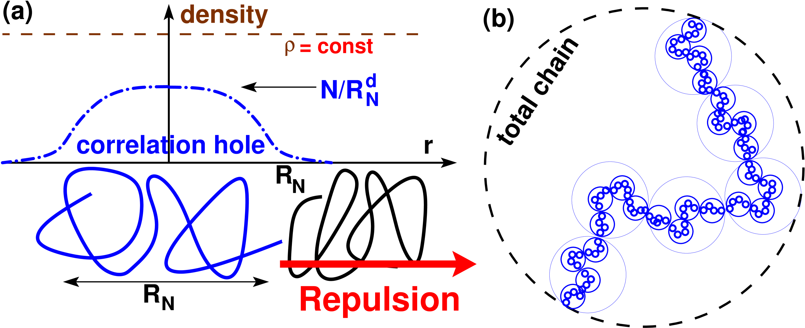
Let us for the clarity of the presentation return to monodisperse chains in the large- limit, i.e. let us assume that and that thus the total monomer density does not fluctuate. On the other hand, composition fluctuations of labeled chains or subchains may certainly occur, however, subject to the total density constraint. Composition fluctuations are therefore coupled and chains and subchains must feel an entropic penalty when the distance between their CM becomes comparable to their typical size ANS03 ; WBJSOMB07 .
As sketched in Fig. 3(a), let us first remind the well-known “correlation hole” effect for two test chains of length in the bath DoiEdwardsBook ; ANS03 . The scaling of their effective interaction under the incompressibility constraint is obtained from the potential of mean force ChandlerBook with being the pair correlation function of the chains, i.e. the probability distribution to find the CM of the second chain at a distance assuming the CM of the first chain at the origin (). Since the correlation hole is shallow for large , expansion of the logarithm leads to
| (49) |
with being the density distribution of the reference chain around its CM. This distribution scales as
| (50) |
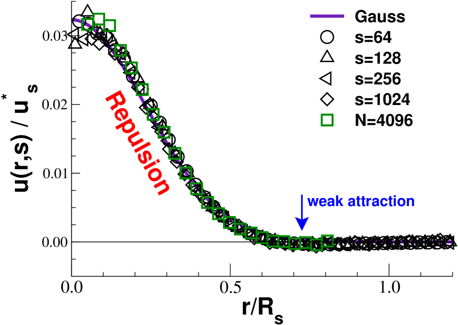
with being the chain self-density, Eq. (1), and a universal function which becomes constant for and decays rapidly for .252525For (to leading order) Gaussian chains must also be Gaussian DegennesBook as indicated by the bold line in Fig. 4. The interaction penalty for two chains at is thus given by
| (51) |
which decreases as in ANS03 ; WBJSOMB07 . Hence, although the incompressibility constraint couples the chains, the correlations become rapidly negligible with increasing chain length in agreement with our discussion in Sec. 1.1.
Interestingly, the above scaling argument does not only hold for chains () but also for the potential of mean force obtained in a similar manner from the pair correlation function of the center-of masses of subchains of arc-length WBJSOMB07 ; WBM07 . Since
| (52) |
the correlation hole effect strongly increases with decreasing , albeit it remains always perturbative in . Note that the subchain correlation hole potential does not depend explicitly on the bulk compression modulus . It is dimensionless and independent of the definition of the monomer unit, i.e. it does not change if monomers are regrouped to form an effective monomer (, ) while keeping fixed.
That the effective correlation hole potential for chains and subchains is more than a heuristic scaling argument can be seen from Fig. 4. We present here the rescaled potential of mean force for chains of length obtained using the BFM algorithm described in Sec. 3.3. The correlation hole potential for the total chains is indicated by the squares. The predicted scaling is confirmed by the perfect data collapse of plotted as function of . Please note that, strictly speaking, for subchains accounts also for the attractive interaction between subchains on the same chain and therefore differs slightly from the effective interaction potential of two independent chains of length . This leads to the (very weak) attractive contribution to for subchains (barely) visible in Fig. 4. However, this additional effect does not affect the scaling on short distances, , which matters here.
2.3.5 Connectivity and swelling
To connect two test chains of length to form a chain of length an effective free energy has to be paid and this repulsion will push the two halves apart from each other ANS03 . We consider next a subchain of length in the middle of a very long chain. All interactions between the test subchain and the rest of the chain are first switched off but we keep all other interactions, especially within the subchain and between the subchain monomers and monomers of surrounding chains. The typical size of the test subchain remains essentially unchanged from the size of an independent chain of the same strand length. If we now switch on the interactions between the tagged subchain and monomers on adjacent subchains of same length , this corresponds to an effective interaction of order as before. (The effect of switching on the interaction to all other monomers of the chain is inessential at scaling level, since these other monomers are more distant.) Since this repels the respective subchains from each other, the corresponding subchain is swollen compared to a Gaussian chain of non-interacting subchains. It is this effect we want to characterize.
2.3.6 Perturbation approach in three dimensions
Let us return to systems of finite dimensionless compressibility but let us focus on subchains of length which are larger than the number of monomers contained in the thermal blob, i.e. we focus on scales where the incompressibility constraint matters. Interestingly, when taken at the subchain correlation hole potential becomes
| (53) |
with being the standard Ginzburg parameter already defined in Eq. (48). Hence, it follows for the subchain correlation hole potential that
| (54) |
Although for real polymer melts as for computational systems large values of may sometimes be found, decreases rapidly with in three dimensions, as illustrated in Fig. 3(b), and standard perturbation calculations can be successfully performed.
As sketched in Sec. 2.4 these calculations consider dimensionless quantities which are defined such that they vanish () if the perturbation potential is switched off and are then shown to scale, to leading order, linearly with . For instance, for the quantity , defined in Eq. (26), characterizing the deviation of the subchain size from Flory’s hypothesis one thus expects the scaling
| (55) |
The -sign indicated marks the fact that the prefactor has to be positive to be consistent with the expected swelling of the chains. Consequently, the rescaled mean-squared subchain size, , must approach the asymptotic limit for large from below. For 3D melts Eq. (55) implies that should vanish rapidly as .262626This is different in thin films where decays only logarithmically ANS03 . Taking apart the prefactors — which require a full calculation — this corresponds exactly to Eq. (10) with a swelling coefficient . Note also that the predicted deviations are inversely proportional to , i.e. the more flexible the chains, the more pronounced the effect. Similar relations may also be formulated for other quantities and will be tested numerically in Sec. 5.
2.4 Perturbation calculation
2.4.1 General approach
We remind that the first-order perturbation calculation of an observable under a dimensionless perturbation potential (defined in units of ) generally reads DoiEdwardsBook
| (56) |
where averages performed over an unperturbed reference system of Gaussian chains are denoted . Obviously, for . For the reduced quantity Eq. (56) simplifies to
| (57) |
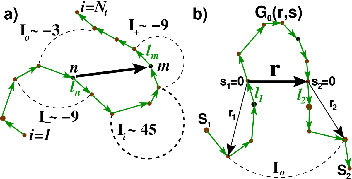
For one may introduce the dimensionless observable which, of course, also obeys Eq. (57). If , as is the case if self-energies and ultra-violet divergencies can be dumped into the reference of , this is consistent with Eq. (55). The observable stands, for instance, for the -th moment of the vector between two monomers and on the tagged chain as shown in Fig. 1 WMBJOMMS04 ; WBM07 or for the scalar product of two bond vectors WJO10 ; ANS10a . If, as in the latter case, we have for linear chains by construction, one only has to compute .
In this subsection we use for the bond length of the unperturbed Gaussian reference chain which may a priori be different from the effective bond length defined and measured according to Eq. (17). The reference bond length is a parameter which may be suitably chosen or adjusted in a Hartree-Fock iteration scheme ThijssenBook (as shown in Sec. 5.3.3) for the specific problem and observable considered. If one is, for instance, interested in predicting the effective bond length for a weakly interacting system, a good trial value for should be the bond length of non-interacting chains on the lattice DoiEdwardsBook . To be consistent the perturbation potential must in this case vanish if the interactions are switched off (). If on the other side the aim is to characterize the deviations from Flory’s ideality hypothesis in incompressible melts () one may naturally set , i.e. one uses as reference the Gaussian chain which fits the chain on large scales (Sec. 2.4.5). Obviously, in this case the perturbation potential must vanish in this low-wavevector limit such that . The last choice for turns out to be the best one in all cases where one does not need to predict the effective bond length but where it can be determined independently by fitting some large scale intrachain property such as the typical chain end-to-end distance .
The perturbation energy for a tagged test chain of length is given by the potential
| (58) |
As further discussed in Sec. 2.4.2, the effective interaction between two monomers of the test chain arises due to the presence of the bath of surrounding chains which screens the direct excluded volume interaction . The calculations are most readily performed in Fourier-Laplace space using definitions given in Sec. 2.2.3. See for instance the calculation presented in Appendix B.2 for the non-Gaussian contribution to the subchain size distribution or Appendix B.4 for the bond-bond correlation function .
2.4.2 Effective interaction potential
We have still to specify the effective monomer interaction in reciprocal space with being the wavevector conjugated to the distance between two monomers and of the tagged chain. Note that in general the test chain length and the mean chain length of the bath may differ. Within linear response the effective pair interaction reads DoiEdwardsBook ; BJSOBW07
| (59) |
The first term stands here for the bare excluded volume interaction between monomers. As we have already stressed above, Eq. (43), thermodynamic consistency requires that is set by the excess contribution to the isothermal compressibility of the solution: ANS05a ; BJSOBW07 ; WCK09 ; GHF95 .272727The bulk modulus only dominates for all in extremely compressible systems where . stands for the ideal chain intramolecular form factor of the bath of chains surrounding the reference chain. According to Eq. (38) the effective interaction depends thus in general on the length distribution of the bath. We remind that for Flory-distributed melts the form factor is given by Eq. (40). Replacing by this corresponds to the Padé approximation, Eq. (37), of the awkward Debye function for monodisperse chains.
Let us first assume that , i.e. we assume in incompressible solutions () and for systems with a well-defined thermal blob (). The effective interaction is then given by
| (60) |
i.e. the effective interaction is given alone by the inverse structure factor of the bath and does not depend explicitly on the compressibility of the solution.282828Since we shall set at the end of calculation and since the effective bond length depends on , the effective potential depends implicitly on . According to Eq. (39) the effective potential becomes in the low-wavevector limit
| (61) |
i.e. for Flory-distributed melts and for monodisperse melts. Long test chains are ruled by which acts as a weak repulsive pseudo-potential with associated Fixman parameter DoiEdwardsBook .292929Characterizing the excluded volume interaction free energy of a chain with itself the Fixman parameter of a chain of length of excluded volume may be defined more generally as Note that for a monodisperse melt of chain length and dimensionless compressibility the Fixman parameter and the Ginzburg parameter become identical, . It follows that
| (62) |
and the chains thus must swell and obey excluded volume statistics DegennesBook ; SchaferBook .303030For this reason an upper bound is indicated, e.g., in Eq. (106). We note that for a Flory-distributed bath Eq. (60) becomes
| (63) |
which can also be used within the Padé approximation () for the calculation of monodisperse systems WMBJOMMS04 ; WBM07 . More importantly, the effective potential becomes for intermediate wavevectors
| (64) |
and this irrespective of the length distribution of the bath. Eq. (64) lies at the heart of the announced power-law swelling of (sub)chains, Eq. (9) or Eq. (55) WMBJOMMS04 ; BJSOBW07 ; WBM07 ; WJO10 .
For later reference in Sec. B.4 we note that for a Flory-distributed bath of finite compressibility the pair potential reads
| (65) |
where following Eq. (44). Allowing to characterize wavevectors below and above , Eq. (65) reduces to Eq. (61) for very low wavevectors and to Eq. (64) in the intermediate wavevector range. In the limit of asymptotically long chains () Eq. (65) becomes DoiEdwardsBook
| (66) |
which corresponds in real space to DoiEdwardsBook
| (67) |
i.e. the effective potential consists of a strongly repulsive part of very short range (), and an attractive part of range stemming from the compression of the reference chain by the bath chains.313131See Fig. II.1 of de Gennes’ book DegennesBook . Using Eq. (66) it follows that
| (68) |
which is commonly taken as a proof that “there is no excluded volume interaction among the segments whose mean separation is larger than ” DoiEdwardsBook . Unfortunately, Eq. (68) does not imply mathematically that all other moments, say the integral over , should also rigorously vanish. It is thus incorrect to state that all possible correlation functions must be short-ranged. However, it remains relevant that vanishes with decreasing wavevector and the same applies for the total perturbation to the Gaussian reference.323232Hence, in the large-scale limit for an observable which suggests for the Gaussian chain reference bond length.
2.4.3 Free energy for high compressibilities
For later use in Sec. 4 we reformulate here a perturbation calculation result obtained long ago by Edwards DoiEdwardsBook using Eq. (66) which allows to predict thermodynamic properties of melts with sufficiently large compressibilities . Integrating twice with respect to the density the osmotic pressure given by Eq. (5.45) or Eq. (5.II.5) of DoiEdwardsBook one obtains for monodisperse melts the free energy per monomer
| (69) | |||||
and being the inverse temperature, the bond length of the Gaussian reference chains and the second virial coefficient of a solution of unconnected monomers. The first term is due to the (essentially constant) intrachain self-energy which shall be discussed in Sec. 4.2. It is due to the reference energy chosen in our numerical model Hamiltonian and it is normally not accessible experimentally. A similar intrachain energy contribution to the free energy arises also from Eq. (5.43) of DoiEdwardsBook if an upper cutoff is introduced for the wavevectors to avoid the ultra-violet divergence. Such an upper cutoff is justified by the discreteness of the monomers of real polymers. This leads necessarily to a non-universal free energy contribution which can be seen as an integration constant with respect to the integration of a measurable property such as the osmotic pressure or the compressibility. The second term in Eq. (69) represents the translational invariance of monodisperse chains of length (van’t Hoff’s law). Due to this contribution the compressibilities depend in general on as will be discussed in Sec. 4.4.333333For general polydisperse melts of given partial densities the ideal gas contribution becomes . The (bare) excluded volume interaction between the monomers is accounted for by the third term. The underlined term in the second line represents the leading correction to the previous term due to the fact that the monomers are connected by bonds summing over the density fluctuations to quadratic order. As one expects DegennesBook , the corresponding correlations of the density fluctuations reduce the free energy by about one per thermal blob of volume . Interestingly, according to Edwards DoiEdwardsBook the chain connectivity, i.e. the presence of attractive forces between bonded monomers, does not change the excluded volume — as one would expect naively — but rather gives rise to an additional term scaling differently with density.343434A free energy contribution may be added to Eq. (69) if one insists on taking as reference for the connectivity contribution to the free energy the limit , i.e. , where the chain connectivity becomes irrelevant. Various thermodynamic properties are readily obtained from the quoted free energy and will be compared with our numerical results in Sec. 4. The underlined density fluctuation contribution to the free energy will be demonstrated numerically from the scaling of the specific heat (Sec. 4.3).
As the reader might have noticed we have written the free energy in Eq. (69) following Edwards assuming for the bare monomer interaction and for the bond length of the Gaussian reference chain. As already alluded to above (Sec. 2.4.1), one would nowadays rather set and using the imposed or measured dimensionless compressibility and the measured effective bond length . However, the choice of Edwards has a clear advantage: and may not be known with sufficient precision while the second virial coefficient and the bond length can always be calculated from the given model Hamiltonian. According to Eq. (5.46) of Ref. DoiEdwardsBook the stated free energy is supposed to hold in the limit where with being the Ginzburg parameter. As we shall see in Sec. 4, this restricts the validity of the related predictions to rather weak values of the (reduced) Lagrange multiplier applied to control the compressibility. In the range of validity of Eq. (69) it turns out that and , i.e. the difference between both parameter choices correspond to irrelevant higher order corrections.
2.4.4 Subchain size distribution and its moments
We turn now to the perturbation calculation predictions of intrachain conformational properties which will be compared with our numerical data in Sec. 5. We focus first on the scale-free wavevector regime for arbitrarily long chains described by the effective interaction potential Eq. (66), i.e. effects related to the chain length distribution are irrelevant. For the observable with we indicate in Fig. 5(a) the different interaction graphs one may compute in real space WMBJOMMS04
| (70) |
The diagram corresponds to the standard graph computed by Edwards for the total chain () DoiEdwardsBook . Consistent with Edwards its leading Gaussian contribution describes how the effective bond length is increased from to under the influence of a small excluded volume interaction inside the subchain between and . Note that all other contributions proportional to correspond to the leading non-Gaussian corrections predicted in Eq. (10). They only depend on and but, more importantly, not on in agreement with the scaling discussed in Sec. 2.3.6. The relative weights of these four contributions are indicated in Fig. 5(a) in units of . The dominant correction stems from the interaction within the subchain. The diagrams and are obviously identical in the scale-free limit.353535Using Eq. (4) it follows that the interactions described by the strongest graph align the bonds and while the others tend to reduce the effect WMBJOMMS04 . As shown in Fig. 5(b), it is better to place the bond pair outside the subchain if one computes directly (Sec. 2.4.6 and Sec. B.4). For symmetry reasons only the interaction graph between the dangling ends matters for the alignment of the bond pair. Both pictures are consistent and lead to the same result. Summing over all contributions this yields
| (71) | |||||
where in the second line we have used the definition already mentioned in Sec. 1.5 and have set
| (72) |
with .
For higher moments of the distribution it is convenient to calculate first the perturbation deviations of the Fourier-Laplace transformation with and to obtain the moments from the coefficients of the expansion of this “generating function” in terms of the squared wavevector . As explained in detail in the Appendix B.2, this leads to a deviation
| (73) |
with and the universal function
| (74) |
which allows to specify all moments of WBM07 .
2.4.5 Adjusting the bond length of the reference chain
The above perturbation result Eq. (72) is of relevance to describe the effect of a weak excluded volume on a reference system of ideal polymer melts with bond length where all interactions have been switched off (). It is expected to give a good estimation for the effective bond length only for a small Ginzburg parameter . For the dense incompressible melts we want to describe the latter condition does not hold and one cannot hope to find a good quantitative agreement with Eq. (72). Note also that large wavevectors contribute strongly to the leading Gaussian term. The effective bond length is, hence, strongly influenced by local and non-universal effects and is very difficult to predict in general (Sec. 5.3).
Our more modest goal is to predict the coefficient of the -perturbation and to express it in terms of a suitable variational reference Hamiltonian characterized by a conveniently chosen and the measured effective bond length (instead of Eq. (72)). Following Refs. Edwards82 ; WBM07 we argue that for dense melts should be renormalized to to take into account higher order graphs.363636The general scaling argument discussed in Sec. 2.3.6 states that we have only one relevant length scale in this problem, the typical subchain size itself. The incompressibility constraint cannot generate an additional scale. It is this size which sets the strength of the effective interaction which then in turn feeds back to the deviations of from Gaussianity. Having a bond length in addition to the effective bond length associated with would imply a second length scale . Restating thus Eq. (73) with the subchain size distribution may be rewritten
| (75) |
and for the -th moment of distribution this yields
| (76) |
which reduces for to Eq. (10) as stated in the Introduction. As a consequence the non-Gaussianity parameters and defined in Sec. 2.2.3 become
| (77) |
and
| (78) |
Eq. (78) can be obtained from Eq. (77) by expanding the second moment () in the denominator of the definition Eq. (27).
2.4.6 Bond-bond correlation function
The bond-bond correlation function is a central property since it allows to probe directly the colored forces acting on the reference chain due to the incompressibility constraint, Eq. (176). Using Eq. (4) may be obtained by differentiating the second moment of the subchain size distribution with respect to the arc-length . For arbitrarily large chains and this yields with as announced in the Introduction.
It is also possible to obtain directly by averaging the observable . Since for linear chains by construction, the task is to compute Eq. (57).373737We remind that for closed cycles the ring closure implies long-range angular correlations even for Gaussian chains, hence for rings to leading order WJO10 . Changing slightly the notations as indicated in Fig. 5(b), we consider two bonds and outside the -segment. The lengths of the two tails of the chains are denoted and . One of the tails, say , may be fixed by the total length of the test chain. Placing the head of the first bond at the origin we consider the correlation function between two bonds separated by the distance . Interestingly, it can be seen by symmetry considerations that does only depend on the effective interaction of the monomers in the first tail with the monomers in the second tail and not on the monomers in the intermediate strand of length . Hence, we need only to calculate one interaction graph as opposed to the four graphs required by the calculation of throught . It is for this reason we have chosen the indicated positions of heads and tails of the bond vectors. With denoting the normalized distribution of the bond vector of the polymer model considered, the interaction graph in real space may be written
| (79) | |||||
where points from the head of the bond to the monomer in the first tail and from the tail of the bond to the monomer in the second dangling chain end. As the -segment is not implied in the perturbation of , the constraint which consists in putting the two points on the same chain and putting a -strand between them introduces, to lowest order, the Gaussian propagator . Using Parseval’s theorem the bond-bond correlation function reads
| (80) |
with being the Fourier transform of .383838It can be shown that for infinite chains and, hence, i.e. for at fixed distance . Note that is a mere technical intermediate quantity which should not be confused with the bond-bond correlation function discussed in Sec. 5.4.2 and Sec. B.5. To simplify the notations we set from the start , i.e. we take the effective bond length as the bond length of the Gaussian reference chain. Although this is not strictly necessary, the calculation in reciprocal space may be strongly simplified by assuming the bond vector distribution to be a Gaussian with . This implies that the chain is perfectly flexible, i.e. .393939The complete formula for systems of general rigidity can be recovered by multiplying the final perturbation calculation result with as may be seen by scaling considerations WJO10 ; ANS10a or by simply comparing the result with the bond-bond correlations obtained using . Under these premises a bond vector may be represented in reciprocal space as
| (81) |
with being the Fourier transformed bond vector distribution.404040For a general bond vector distribution one may expand at low momentum as indicated in Sec. B.1. Let us denote the wavevectors conjugated to the bonds and by and , respectively. The Fourier transform of the observable thus reads
| (82) |
Using Eq. (82) for the observable and Eq. (66) for the interaction potential for Flory-distributed systems of given compressibility one may integrate Eq. (80) in reciprocal space as shown in Appendix B.4. In the limit of very long chains () one obtains in dimensions WCK09
| (83) |
as a function of the reduced arc-length with being the complementary error function abramowitz . As one expects, Eq. (83) reduces to Eq. (9) for large , i.e. irrespective of the compressibility the bond-bond correlation function behaves as in the incompressible limit. In the opposite limit where the structure within the thermal blob is probed Eq. (83) corresponds to the weaker decay
| (84) |
This regime is consistent with the classical expansion result of the chain size in terms of the Fixman parameter WCK09 .414141Omitting all prefactors we remind DoiEdwardsBook that to leading order . Using Eq. (4) it follows that . We therefore refer to this limit as the “Fixman regime”.
2.4.7 Finite chain size effects
To describe properly finite chain size corrections, Eq. (64) must be replaced by the general formula Eq. (59). For monodisperse chains () the form factor is given by Debye’s function Eq. (36). This approximation allows in principle to compute, e.g., the mean-squared total chain end-to-end distance, . One verifies readily (see DoiEdwardsBook , Eq. (5.III.9)) that the effect of the perturbation may be expressed as
| (85) |
We take now first the integral over . In the remaining integral over small wavevectors contribute to the -swelling while large renormalize the effective bond length of the dominant Gaussian behavior linear in (as discussed above). Since we wish to determine the non-Gaussian corrections, we focus on small wavevectors , i.e. the effective interaction potential is given by Eq. (60). We thus continue the calculation using with being Debye’s function and . This allows us to express the swelling as
| (86) |
We have set here in agreement with the renormalization of the reference bond length discussed above. The numerical integral over is slowly convergent at infinity. As a consequence the estimate may be too large for moderate chain lengths. In practice, convergence is not achieved for values corresponding to the screening length .
We remark finally that for various properties numerical integration can be avoided replacing the Debye function by the Padé approximation, Eq. (63). This has been done for instance for the calculation of finite chain size effects for the bond-bond correlation function discussed in Sec. 5.4.1.424242It is interesting to compare the numerical value obtained for the r.h.s. of Eq. (86) with the coefficients one would obtain by computing Eq. (85) either with the effective potential for infinite chains given by Eq. (66) or with the Padé approximation, Eq. (63). Within these approximations of the full linear response formula, Eq. (59), the coefficients can be obtained directly without numerical integration yielding overall similar values. In the first case we obtain and in the second WBM07 . While the first value is clearly not compatible with the measured end-to-end distances, the second yields a reasonable fit, especially for small .
3 Bond-fluctuation model
3.1 Introduction
The theoretical predictions sketched above should hold in any dense homopolymer solution assuming that the chains are asymptotically long, i.e. at least and even better . The computational challenge is to equilibrate and to sample such configurations using an as simple as possible coarse-grained model for polymer melts VanderzandeBook ; BWM04 . In this study we use the BFM, an efficient lattice MC algorithm proposed as an alternative to single-site self-avoiding walk models by Carmesin and Kremer in 1988 BFM . As illustrated in Fig. 6, the key idea of the model is to increase the size of the monomers which now occupy whole unit cells on a simple cubic lattice connected by a specified set of allowed bond vectors. While the multitude of possible bond lengths and angles allows a better representation of the continuous-space behavior of real polymer solutions and melts, the model remains sufficiently simple retaining thus the computational efficiency of lattice models without being plagued by ergodicity problems BWM04 . The BFM algorithm has been used for a huge range of problems addressing the generic behavior of long polymer chains of very different molecular architectures and geometries: statics and dynamics of linear Paul91a ; Paul91b ; WPB92 ; WPB94 ; Shaffer94 ; Shaffer95 ; MWBBL03 ; MM00 ; WMBJOMMS04 ; WBJSOMB07 ; BJSOBW07 ; WBM07 ; MWK08 ; WCK09 ; Wittmann90 ; DeutschDickman90 ; Deutsch ; MP94 ; WM94 ; Freire02 and cyclic MWC96 ; MWC00 ; MWB00 homopolymer melts, polymer blends MarcusT3D95 ; Blends99 ; Cavallo03 ; Cavallo05 ; Kumar03 , gels and networks Sommer05 , glass transition OWBK97 ; BBP03 ; Mateo05 ; Freire08 ; Mateo09 , polymers and copolymers at surfaces CopolySurface99 ; Paul08 , brushes WJJB94 ; KBWB96 ; WCJT96 , thin films combpoly00 ; MBB01 ; MM02 ; MBDB02 ; CMWJB05 , equilibrium polymers Milchev95 ; WMC98a ; WMC98b ; papEPslit and other problems related to monomer and chain self-assembly Micelles06 ; Cavallo08 . For recent reviews on the BFM algorithm see Refs. BWM04 ; BFMreview05 .
Throughout this paper all lengths and densities are given in units of the lattice constant , time scales are given in units of the Monte Carlo Step (MCS) and Boltzmann’s constant is set to unity. Taking apart some paragraphs in Sec. 4 we assume a temperature . If not specified otherwise the chains are monodisperse of length .
We define first the classical BFM variant without monomer overlap () and explain then how dense configurations may be obtained using a mix of local and global MC moves (Sec. 3.3). The generalization of the BFM Hamiltonian to finite monomer overlap penalties is presented in Sec. 3.4. Finally, we turn in Sec. 3.5 to polydisperse equilibrium polymer systems with annealed size distribution.
3.2 Classical BFM without monomer overlap
The classical implementations of the BFM idea do not permit monomer overlap, i.e. each monomer occupies exclusively a unit cell of lattice sites on a -dimensional simple cubic lattice BFM ; BWM04 ; BFMreview05 . The fraction of occupied lattice sites is thus with being the -dimensional monomer number density. A widely used choice for the allowed bond vectors for the 3D variant () of the BFM introduced by the Mainz condensed matter theory group around K. Binder Paul91a ; Paul91b ; WPB92 ; WPB94 ; Wittmann90 ; DeutschDickman90 ; Deutsch ; MP94 ; WM94 is given by
| (87) |
where stands for all the possible permutations and sign combinations of a lattice vector. This corresponds to 108 different bond vectors of 5 possible bond lengths (, , , , ) and angles between consecutive bonds. The smallest angles do not appear for the classical BFM because excluded volume forbids the sharp backfolding of bonds. If only local hopping moves to the nearest neighbor sites are performed — called “L06 moves” WBM07 — this set of vectors ensures automatically that polymer chains cannot cross. (The corresponding “L04 moves” for the 2D variant of the BFM are represented in Fig. 6(b) by filled circles.) Topological constraints, e.g. in ring polymers MWC96 ; MWC00 ; MWB00 or polymer gels Sommer05 , hence are conserved.434343Following Paul91a ; Paul91b we keep lists of the monomer positions in absolute space, their corresponding lattice positions and of the indices of the bond vectors connecting the monomers of the chains. Since the bond vector index can be encoded as a byte, this allows a rather compact storage of the configurations. Predefined tables allow the rapid verification of the excluded volume condition on the periodic lattice. Following Müller MarcusT3D95 ; BFMreview05 we use a Wigner-Seitz representation of the cubic lattice where a cube is not represented by 8 entries on the lattice but just by one variable in the cube center. This variable can be a boolean if we are only interested in homopolymers or an integer if we deal with a mixture of different monomer types. Although the Wigner-Seitz representation of the BFM algorithm is about a factor 3 slower than the original implementation, it has the advantage that the code becomes more compact and can be more readily adapted to the various polymer architectures or interaction potentials of interest.
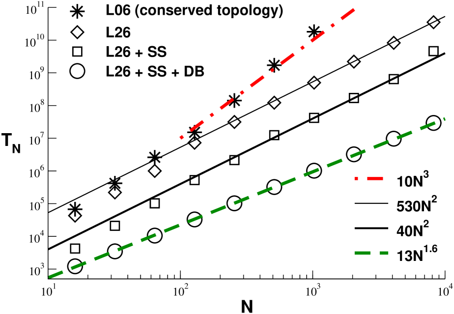
Consequently, several authors report reptation-type dynamics for chain lengths at a standard “melt” volume fraction Paul91a ; Paul91b ; KBMB01 ; HT03 .444444The BFM version by Shaffer Shaffer94 ; Shaffer95 assumes a different bond vector set which leads to a higher chain stiffness and, hence, to smaller values of the entanglement length . Note that if one applies a local stiffness potential, as discussed Sec. 2.2, one finds quite generally that topological effects become more pronounced WPB92 ; MWC00 ; MWB00 . As may be seen from the stars indicated in Fig. 7, the relaxation time obtained using L06 moves WBM07 becomes similar to the reptation theory prediction (dash-dotted line). We have used here — as elsewhere if not stated otherwise — periodic simulation boxes of linear dimension containing monomers. This large system size allows to eliminate finite-size effects even for the longest chain lengths studied. The relaxation time has been estimated here (for historical reasons) using the self-diffusion coefficient obtained either from the monomer MSD or the chain CM MSD . Other operational definitions of exist Paul91b ; KBMB01 which lead to similar, vertically slightly shifted results. The last data point for has to be taken with care as usual in computational as in experimental studies FeynmanJoking . Being obtained by extrapolation using the expected shape of in log-linear coordinates, it corresponds to a lower bound for . Note that the relaxation time appears thus to increase even more strongly with than the standard reptation theory predicts DoiEdwardsBook . We do not pursue this issue here (which has also been observed in MD simulations) the important point being merely that local topology conserving moves are too inefficient to equilibrate and sample large- polymer melts.
Note that the classical BFM without monomer overlap and using L06 moves is strictly speaking not ergodic, since some configurations may be easily constructed which are not accessible starting from an initial configuration of stretched linear chains. Although topology conservation is irrelevant for the present work (taking apart the preliminary results presented in Sec. 6.5) we keep the set of allowed bond vectors, Eq. (87), for consistency with previous work.
3.3 Local and global topology violating MC moves
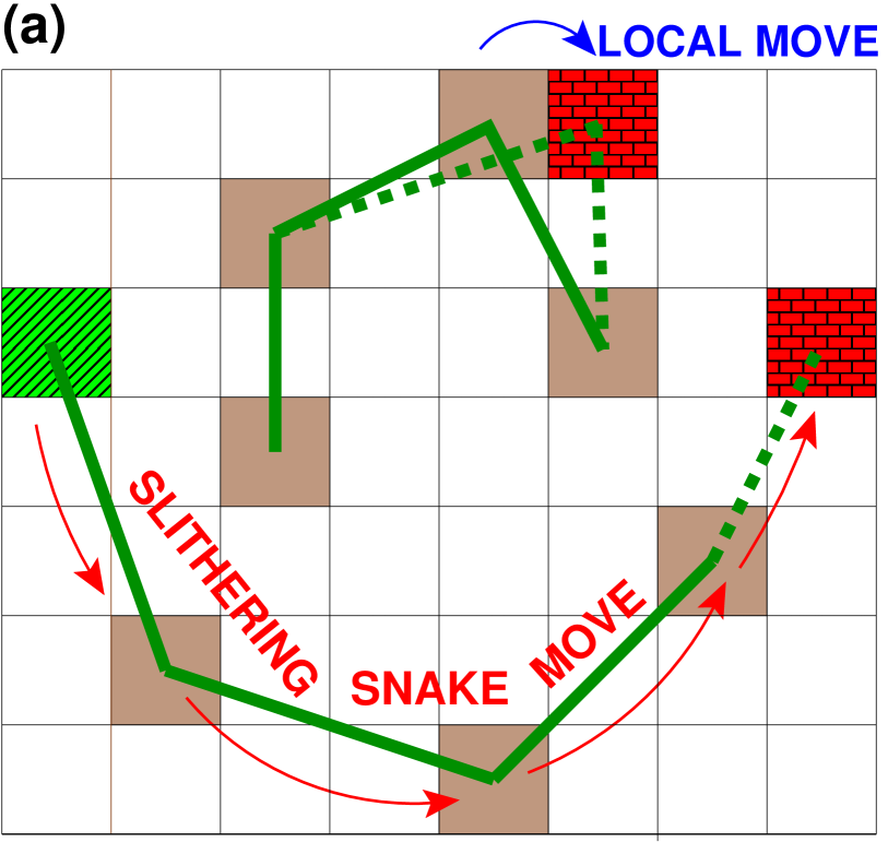
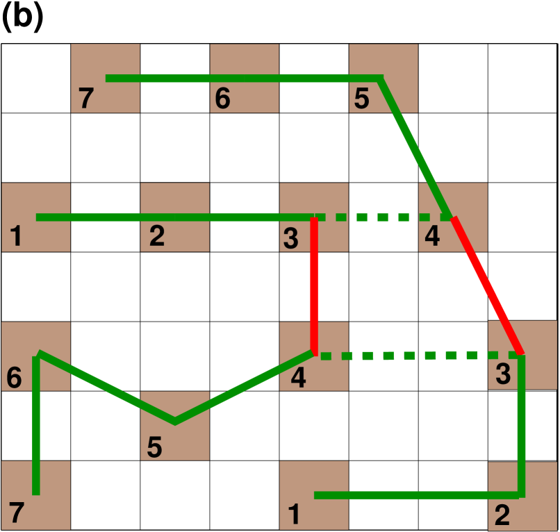
To equilibrate and sample BFM melts such as the ones presented in Fig. 7, we have replaced the realistic but very slow L06 moves by a mix of local topology violating so-called “L26 moves” WBM07 with global “slithering snake” Kron65 ; Wall75 ; MWBBL03 and “double bridging” Theodorou02 ; dePablo03 ; Auhl03 ; BWM04 MC moves as shown in Fig. 8.
3.3.1 Local L26 moves
Already the use of local moves to the next and next-nearest lattice sites surrounding the current monomer position [Fig. 6(b)] dramatically speeds up the relaxation dynamics, especially for , as can be seen from the diamonds indicated in Fig. 7. Since the dynamics is to leading order of Rouse-type, as further discussed in Sec. 6, the diffusion coefficient can readily be estimated from the CM MSD even for our largest chains with . As shown in Fig. 7, we find for L26 dynamics. This is, of course, still prohibitive for the longest chains we aim to characterize.
L26 moves yield configurations not accessible with L06 moves. Concerning the static properties both system classes are practically equivalent. This has been confirmed by counting the number of monomers which become “blocked” (in absolute space or with respect to an initial group of neighbor monomers) once one returns to the L06 scheme. Typically, we find about 10 blocked monomers for a system of monomers WBM07 . While the few blocked monomers are irrelevant for static properties they obviously matter if dynamical properties are probed.454545The same problems arise if slithering snake or double bridging moves are used to equilibrate the configurations.
3.3.2 Slithering snake moves
In addition to these local moves one slithering snake move per chain is attempted on average per MCS corresponding to the displacement of monomers along the chain backbone, as sketched in Fig. 8(a). Note that in our units two displacement attempts per MCS are performed on average per monomer, one for a local move and one for a snake move.464646It is computationally more efficient for large to take off a monomer at one chain end and to paste it at the other leaving all other monomers unaltered. Before static or dynamical measurements are performed the original order of the monomers must then be restored. Interestingly, a significantly larger slithering snake attempt frequency would not be useful since the relaxation time of snakes without or only few local moves increases exponentially with mass as shown in Deutsch85 ; MWBBL03 due to the correlated motion of snakes expected in analogy to the activated reptation limit for real polymer melts mentioned in Sec. 1.4 ANS97 ; ANS98 . In order to obtain an efficient free snake diffusion [with an -independent curvilinear diffusion coefficient and MWBBL03 ; Wall75 it is important to relax density fluctuations rapidly by local dynamical pathways. As shown in Fig. 7 (squares), we find a much reduced relaxation time which is, however, still inconveniently large for our longest chains. Note that most of the CPU time is used by the local moves and the computational load per MCS remains -independent.
3.3.3 Double bridging moves
Double bridging (DB) moves are found to be very useful at high densities and help us to extend the accessible molecular masses close to . As for slithering snake moves we use all bond vectors to switch chain segments between two different chains. Only chain segments of equal length are swapped to conserve monodispersity. Topological constraints are again deliberately violated. Since more than one swap partner is possible for a selected first monomer, delicate detailed balance questions arise BWM04 . This is particularly important for short chains. To avoid the computation of weights BWM04 one simple solution to this problem is to refuse all moves with more than one swap partner.474747Since we have a finite number of possible BFM bonds an even simpler option is to select randomly one bond vector for a given first monomer at a lattice position and to check whether a suitable monomer of another chain exists at . Obviously, using only one instead of 108 bonds reduces the number of DB moves performed, but since correlated moves forth and back in topology space are pointless, this is not of disadvantage. The configurations are screened with a frequency for possible DB moves where we scan in random order over the monomers. The frequency should not be too large to avoid (more or less) immediate back swaps and monomers should move at least over a couple of lattice constants between subsequent DB moves. In the example presented in Fig. 7 (spheres) a frequency is used. Empirically it is found that using the diffusion coefficient obtained from the monomer MSD . For this corresponds to MCS. This allowed us even for the largest chains to observe monomer diffusion over several within the MCS which were feasible in 2007 on our XEON-PC processor cluster WBM07 . The influence of on the performance has yet not been explored systematically, but preliminary results suggest smaller DB frequencies for future studies. The power-law exponent remains robust as is also confirmed by MD simulations of a bead-spring model coupled to DB moves WBM07 . This finding begs for a systematic theoretical investigation.
| 0.0 | 2.718 | 2.72 | 0.2109 | 0.032 | 0.065 | |
| 0.01 | 209 | 2.718 | 2.80 | 0.2109 | 0.030 | 0.062 |
| 0.03 | 67 | 2.718 | 2.85 | 0.2099 | 0.028 | 0.060 |
| 0.1 | 22 | 2.719 | 2.92 | 0.2067 | 0.024 | 0.058 |
| 0.3 | 7.1 | 2.720 | 3.01 | 0.1992 | 0.021 | 0.050 |
| 1 | 2.4 | 2.721 | 3.13 | 0.1796 | 0.015 | 0.040 |
| 3 | 0.85 | 2.721 | 3.21 | 0.1432 | 0.008 | 0.024 |
| 10 | 0.32 | 2.670 | 3.24 | 8.8E-02 | 0.003 | 0.009 |
| 30 | 0.25 | 2.638 | 3.24 | 7.2E-02 | 0.0013 | 0.004 |
| 100 | 0.25 | 2.636 | 3.24 | 6.9E-02 | 0.0010 | 0.003 |
| 0.25 | 2.636 | 3.24 | 6.9E-02 | 0.0010 | 0.003 |
3.3.4 Summary of static properties
Some static properties obtained at our reference volume fraction assuming no monomer overlap () are indicated in Table 1. Averages are performed over all chains and typically 1000 configurations. Taking apart the systems for , chains are always much smaller than the linear box size . In the large -limit we obtain an average bond length , a root-mean-squared bond length and an effective bond length as will be shown below in Sec. 5.3. This corresponds to a ratio and, hence, to a persistence length . The swelling coefficient defined in Sec. 1.5 is thus . Especially, we find from the zero wavevector limit of the total structure factor a dimensionless compressibility [Eq. (43)] which compares well with real experimental melts. From the measured bulk compression modulus and the effective bond length one estimates a Ginzburg parameter . Following Ref. ANS05a the interaction parameter is supposed here to be given by the full inverse compressibility and not just by the second virial coefficient of the BFM monomers DeutschDickman90 .
3.4 BFM with finite excluded volume penalty
3.4.1 Definition of Hamiltonian
Fig. 6 shows how finite energy penalties may be introduced in the BFM algorithm WCK09 . The overlap of two cube corners on one lattice site () corresponds to an energy cost of , the full overlap of two monomers () to an energy . More generally, with being the total number of interacting cube corners the total interaction energy of a configuration is
| (88) |
With the energies of the final () and the initial configurations () we accept a proposed MC move according to the Metropolis criterion with a probability LandauBinderBook ; KrauthBook . If the overlap penalty is the only energy scale as in the studies presented here, one may, of course, either vary the overlap parameter or the temperature . For the presentation of thermodynamic properties in Sec. 4 it will be more naturally to use as the control parameter and to fix arbitrarily . The inverse temperature and the dimensionless overlap strength are thus numerically equal. (Both notations are kept for dimensional reasons and for future generalization to models with more than one energy scale.) In other parts of this review, especially Sec. 5 and Sec. 6, it will be more natural to set temperature to unity, , using the overlap strength as the control parameter.
3.4.2 Second virial coefficient
To illustrate this finite excluded volume interaction we indicate the second virial of an imperfect gas of unconnected monomers, , which is shown below to be useful for roughly characterizing the effective strength of the potential. stands for a possible lattice vector between the centers of two interacting cubes. It is easy to see that there are 8 vectors corresponding to as shown in Fig. 6(a), 12 to (overlap of two cube corners), 6 to (overlap of two faces), and 1 to (full overlap). Setting this leads to a second virial
| (89) | |||||
given in units of the lattice cube volume . We note that the second virial becomes constant, , for large as expected DeutschDickman90 . This second virial coefficient is about half the effective bulk modulus indicated above. In the opposite limit we have
| (90) |
We shall see in Sec. 4.4 that in this limit.
3.4.3 Implementation
Since a lattice site may be occupied now by more than one monomer, it is not possible to use a compact boolean occupation lattice as for the classical BFM. Instead we have mapped Eq. (88) onto a Potts spin model LandauBinderBook
| (91) |
with constant monomer number . We use the Wigner-Seitz representation of the BFM on the cubic lattice MarcusT3D95 ; BFMreview05 where an integer spin variable counts the number of BFM monomers () with cubes centered at a Wigner-Seitz lattice position . Since we have now to compute the interaction between cube centers instead of cube corners, the coupling constant characterizing the interaction between two spins depends only on the relative distance :
| (92) |
Since the interaction is still short-ranged and the values of are readily tabulated, this remains an efficient rendering of the monomer interactions. Note that the first term on the r.h.s. of Eq. (91) contains a constant self-interaction contribution of the monomers with themselves for , which is subtracted by the second term.484848Attractive interactions similar to the ones used in MarcusT3D95 ; Blends99 ; Cavallo03 ; Cavallo05 may be easily added to the Potts spin formulation of the soft BFM. The simulation of polymer blends requires additional Potts spin lattices as the two lattices used to obtain the chemical potential in Sec. 4.5.
| 0.5 | 0.32 | 2.670 | 3.24 | 8.8E-02 | 0.003 | 0.009 |
| 0.25 | 1.1 | 2.709 | 3.65 | 0.1455 | 0.004 | 0.018 |
| 0.125 | 3.3 | 2.725 | 3.95 | 0.1664 | 0.004 | 0.023 |
| 0.0625 | 9.5 | 2.731 | 4.38 | 0.1729 | 0.004 | 0.027 |
| 0.03125 | 26 | 2.733 | 4.77 | 0.1749 | 0.004 | 0.035 |
3.4.4 Equilibration and system properties
As start configurations we have used the equilibrated BFM configurations without monomer overlap () described in Sec. 3.2 WBM07 . As one may expect, the configurational properties are found essentially unchanged for (Table 1). Local L26-moves need to be added to the snake moves for . Otherwise the slithering snake motion will become ineffective MWBBL03 . Simple slithering snakes without local moves are sufficient, however, for smaller penalties. We have crosschecked our results in this regime for and using boxes of linear size by starting our simulations with Gaussian chains at and increasing then the penalty. Table 1 present some system properties obtained for our reference volume fraction such as dimensionless compressibility or the effective bond length . Averages are performed over all chains and at least 100 configurations. The chain lengths , and have been studied with particular care. Density effects have been studied more briefly. As will be discussed in Sec. 4.2, we have sampled weak overlap penalties () for to investigate the intrachain contributions to the mean energy. We have also probed various densities for and as summarized in Table 2. This was done to check for density effects on the deviations to Rouse dynamics as discussed in Sec. 6.4.
3.5 BFM with annealed mass distribution
3.5.1 Motivation and context
As discussed above (Fig. 7), the equilibration and sampling of strictly monodisperse polymer melts is a delicate issue. An elegant way to test the computed conformational properties is given by associating a finite “scission energy” to each bond which has to be paid if a bond is broken CC90 ; Milchev95 ; WMC98a ; WMC98b ; Milchev00 ; HXCWR06 ; papEPslit . Since we are only interested here in linear polymer melts, the formation of closed cycles and the branching of the chains is not permitted.494949In systems of experimental relevance closed cycles are suppressed by the non-negligible rigidity of the chains SW99 ; MWL00b ; WMSB00 . As sketched in Fig. 9, we relax thus the constraint that bonds can never break, i.e. that the connectivity matrix (defining which monomers are connected by BFM bonds) is quenched, and allow the polymerization of the chains and their respective monomers to take place under condition of chemical equilibrium. Such systems of self-assembled EP are not only useful for computational purposes but are also of high experimental relevance.505050In the surfactant literature CC90 EP are often referred to as “living polymers” (LP) although this is potentially confusing since they are distinct from systems that polymerize stepwise, in the presence of a fixed number of initiators, for which this term has previously been reserved Szwarc56 . Since LP are held together by strong covalent carbon-to-carbon bonds, they do not break in the middle of the polymer chain.

An important example sketched in Fig. 9(a) is that of some surfactant molecules forming long giant worm-like micelles which break and recombine constantly at random points along the sequence CC90 ; Israela . Similar systems of EP are formed by liquid sulfur Scott65 ; Wheeler80 , selenium Faivre86 and some protein filaments OozawaBook . Although with respect to their static properties EP behave very much like quenched polymers, the constant reorganization of the chain connectivity offers an additional relaxation pathway reducing strongly the relaxation times CC90 ; Faivre86 ; Milchev00 ; HXCWR06 . Obviously, EP are intrinsically polydisperse with an annealed length distribution minimizing the free energy of the system (Sec. 2.2). Since both the bonding energy per chain and all other free energy contributions to the chain chemical potential are extensive with repect to the chain length — at least according to Flory’s ideality hypothesis — one expects a Flory distribution decreasing exponentially with chain length .
3.5.2 Spatial monomer moves
The EP systems presented in this study have been obtained with the classical BFM algorithm without monomer overlap (, ) at the standard melt volume fraction . Using again the Wigner-Seitz representation we mark (only) the index of each monomer on the periodic lattice of linear size . Thus the indices of the monomers in the neighborhood of a reference monomer are readily obtained which is helpful for the recombination of bonds described below. Only local L06 or L26 monomer moves have been used since the breaking and recombination of the chains reduce the relaxation times dramatically compared to monodisperse systems HXCWR06 . Additional global MC moves as described in Sec. 3.3 may be added, however, in future studies.
3.5.3 Connectivity pointer list
Self-assembled EP are only transient objects and it is thus inefficient to base the data structure on the chains Milchev95 , rather it should be based on the (saturated or unsaturated) bonds of each monomer WMC98b . As sketched in Fig. 9(b), this allows via a linear pointer list between the bonds to avoid all sorting procedures. Using the assumption that no branching of chains is allowed, the two (possible) bonds of each monomer are called and . No specific meaning (or direction) is attached to the sign: this is merely a convenience for finding the monomer from the bond list: . Pointers are taken to couple independently of sign and the bonds are coupled by means of a pointer list in a completely transitive fashion. Only two simple operations are thus required for breaking or recombining bonds. Unsaturated bonds at chain ends point to NIL. Only these bonds may recombine. A minor caveat attached to this data structure arises if the ends of a given chain are not allowed to bind together as in the presented studies. Since there is no direct chain information in the data structure we have to check this constraint before every recombination by working up the pointer list which only adds four lines to the source code.515151For higher the simulation becomes actually faster per MCS since the number of recombinations goes down like the squared density of unsaturated end monomers WMC98b .
3.5.4 Connectivity altering moves
As sketched in Fig. 9(a), EP systems are not only characterized by the monomer density and the finite scission energy which determine the static properties but also by a barrier height which only influences the scission and recombination rates. This barrier is taken into account by setting an attempt frequency for choosing randomly one bond ibond out of the bonds of the system. This frequency is a convenient tool for testing the dynamics of EP at different lifetimes of the chains Milchev00 ; HXCWR06 ; Oshaug95 although for the static properties discussed the choice of is irrelevant. The bond corresponds to a monomer at a position . Depending on whether the bond is saturated or unsaturated we try to break it or to connect it to a suitable nearby unsaturated monomer. A delicate detailed balance problem arises HXCWR06 if unsaturated monomers are available for recombination (the no-closed-cycle condition having been verified). If one chooses now one of these monomers at random, a weight has to be taken into account for the reverse breaking process. Choosing in addition to the reference bond a trial bond vector allows to avoid these weights. If is unsaturated one searches for an unsaturated monomer only at the position (taking into account the periodicity of the lattice). Since monomer overlap is forbidden there is at most one unsaturated monomer at this position. If this is case and if no closed cycle is formed, the recombination is accepted since the energy change is . To satisfy detailed balance a saturated bond can therefore only be broken if its bond vector is identical to the trial bond . Applying the Metropolis algorithm LandauBinderBook a scission is performed whenever the value of a random number between 0 and 1 is smaller than . The fact that we only probe one lattice vector for possible recombinations and not all possible obviously strongly reduces the number of recombination and scission events. However, since we are interested in uncorrelated changes of the connectivity list, a broken monomer must anyway move over a certain distance, say , before a new recombination attempt is made. Otherwise there is a strong chance that the newly created chain end monomer recombines with its previous partner Milchev00 ; HXCWR06 ; Oshaug95 .
| 1 | 6.4 | 11.9 | 2.632 | 12.6 | 5.2 |
|---|---|---|---|---|---|
| 2 | 10.4 | 19.7 | 2.633 | 16.5 | 6.8 |
| 3 | 16.8 | 32.4 | 2.633 | 21.6 | 8.8 |
| 4 | 27.5 | 53.4 | 2.634 | 28.1 | 11.4 |
| 5 | 44.9 | 87.9 | 2.634 | 36.3 | 14.8 |
| 6 | 73.7 | 145 | 2.634 | 46.9 | 19.1 |
| 7 | 121 | 239 | 2.634 | 60.7 | 24.7 |
| 8 | 199 | 394 | 2.634 | 77.9 | 31.8 |
| 9 | 328 | 650 | 2.634 | 102 | 41.4 |
| 10 | 538 | 1075 | 2.634 | 129 | 52.7 |
| 11 | 887 | 1766 | 2.634 | 165 | 67.7 |
| 12 | 1453 | 4747 | 2.634 | 217 | 88.1 |
| 13 | 2390 | 4747 | 2.634 | 270 | 110 |
| 14 | 3911 | 7868 | 2.634 | 348 | 143 |
| 15 | 6183 | 12272 | 2.634 | 426 | 184 |

3.5.5 Some computational results
As summarized in Table 3, we have sampled EP systems with scission energies up to , the largest energy corresponding to a mean chain length . As for the athermal classical monodisperse BFM systems we obtain a dimensionless compressibility , an effective bond length and a swelling coefficient . As discussed in Sec. 2.2.2 one expects EP melts to be Flory distributed [Eq. (20)] if the chemical potential of the chains is extensive with respect to their mass, . The main panel of Fig. 10 presents the normalized length distribution for different scission energies as indicated. A nice data collapse is apparently obtained if is plotted as a function of the reduced chain length using the measured mean chain length . At first sight, there is no sign of deviation from the exponential decay indicated by the solid line. The mean chain length itself is given in panel (b) as a function of together with some higher moments of the distribution. As indicated by the dashed line, we find as expected from Eq. (23) CC90 ; WMC98b . The data presented in the first two panels of Fig. 10 is thus fully consistent with older computational work Milchev95 ; WMC98a ; WMC98b ; Milchev00 ; HXCWR06 ; Kroeger96 ; Padding04 which has let us to believe (incorrectly) that Flory’s ideality hypothesis must hold rigorously. Closer inspection of the histograms reveals, however, deviations for small . As can be seen from panel (c), the probability for short chains is reduced with respect to the Flory distribution (solid line). We shall further investigate this depletion in Sec. 4.6.
We note finally that all EP systems presented here have been sampled within 4 months while the sample of monodisperse configurations for alone required about 3 years on a similar XEON processor. EP are therefore very interesting from the computational point of view, allowing for an efficient test of theoretical predictions.
4 Thermodynamic properties of BFM melts
4.1 Introduction
To characterize the soft BFM model introduced in Sec. 3.4 we will first investigate thermodynamic properties such as the mean overlap energy per monomer , the specific heat , the dimensionless compressibility or the excess chain chemical potential as functions of the reduced overlap strength . For the small- limit these properties have been calculated long ago by Edwards DoiEdwardsBook as summarized in Eq. (69). Various thermodynamic properties obtained from the quoted free energy will be compared with our numerical results WCK09 . To demonstrate that deviations from Flory’s ideality hypothesis are also present in thermodynamic properties we will investigate in detail in Sec. 4.6 the chemical potential in systems of annealed EP using the classical BFM algorithm without monomer overlap.
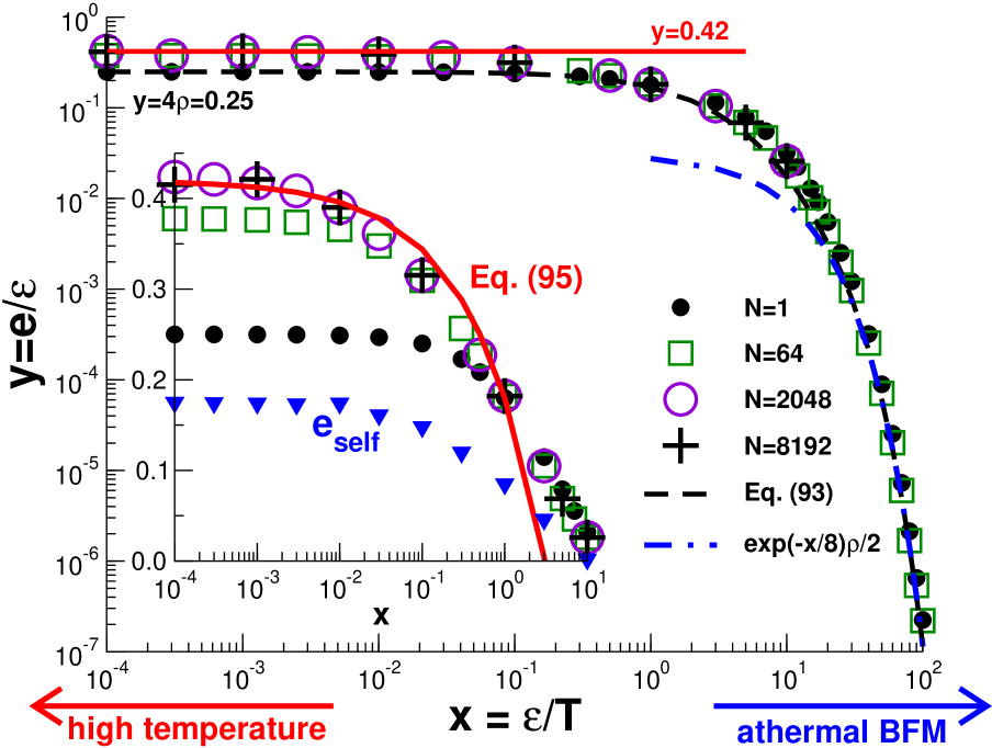
4.2 Mean overlap energy
From the numerical point of view the simplest thermodynamic property to be investigated here is the mean interaction energy per monomer, , due to the Hamiltonian, Eq. (88). Fig. 11 presents the dimensionless energy for BFM melts () for different chain length . Decreasing the overlap strength starting from configurations obtained using the classical BFM (Sec. 3.3), the interaction energy increases first exponentially for large and levels off for where the monomers freely overlap. The data for unconnected beads () represented by the filled spheres and polymer chains () are broadly speaking similar, especially for large overlap penalties, . Interestingly, the mean energy of polymer melts increases more strongly for as can be seen better from the log-linear data representation chosen in the inset of Fig. 11. Also shown in the inset is the mean intrachain self-energy per monomer (filled triangles) obtained for the largest chain length available for a given . In fact about half of the energy of polymer melts for all is due to the self-interactions of the chains WCK09 . For the self-energy becomes which is exactly the observed energy difference between polymer and bead systems.
Before addressing this point let us consider the energy of soft BFM beads () for which the second virial coefficient has been given in Eq. (89). Since the mean energy becomes to leading order McQuarrieBook
| (93) | |||||
corresponding to the first term in the third line of Eq. (69). Eq. (93) is represented by the dashed line in Fig. 11. It corresponds to an Arrhenius behavior with for (dash-dotted line) and to for . This simple formula predicts well the bead data over the entire range of and also yields a remarkable fit for polymer chains with larger overlap penalties.
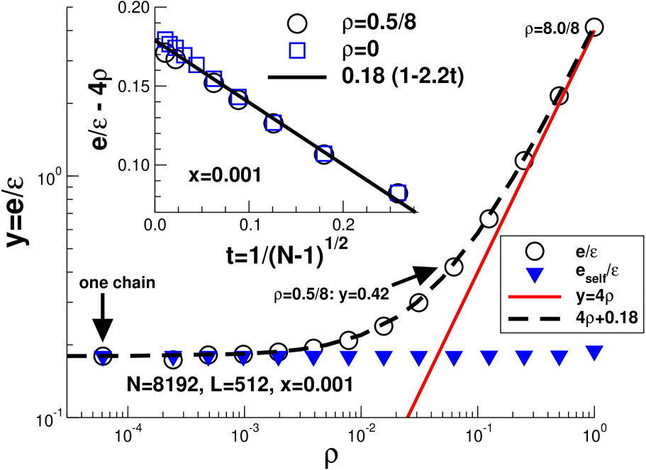
The energy difference between polymer chains and beads for is accounted for by the first free energy contribution indicated in Eq. (69). This contribution is further investigated in Fig. 12 presenting data for such small that the entropy dominates all conformational properties. The self-energy of a chain is thus given by the probability that a random walk of BFM bonds returns to a relative position with respect to a reference monomer at . Hence,
| (94) |
where the first sum runs over all positions with non-vanishing coupling constant as defined in Eq. (92). The probability and the weights can be tabulated in principle for small . Since the return probability decreases strongly with , these model-specific small- values dominate the integral, Eq. (94). As can be seen from the inset of Fig. 12 for single chains (), for large . The weak -dependence visible in the panel stems from the upper integration boundary over the Gaussian return probability which leads to a chain length correction linear in (bold line). Also shown in the panel are energies for our reference density . They are shifted vertically by the mean field energy assuming that density fluctuations of different chains do not couple. The main panel presents the mean energy and the mean self-energy as functions of the density for chains of length . The self-energy (triangles) stays essentially -independent. The total interaction energy sums over the self-energy and mean-field energy contributions as shown by the dashed line. The self-energy contribution can only be neglected for volume fractions larger than unity.
Summarizing Eqs. (69) and (90) the energy should scale to leading order in as
| (95) |
where the two -independent contributions have already been discussed above. The underlined term stems from the density fluctuation contribution in Eq. (69). Eq. (95) is indicated by the bold line in the inset of Fig. 11. It yields a reasonable description for small . Since the energy is dominated by the two constant contributions to Eq. (95) for and since higher expansion terms become relevant for , the predicted -decay corresponds unfortunately only to the small- regime. To show that it is indeed the density fluctuation term which dominates the temperature dependence for we will consider now the specific heat , i.e. the second derivative of the free energy with respect to .
4.3 Energy fluctuations

The fluctuations of the interaction energy are addressed in Fig. 13 displaying the enthalpic contribution to the specific heat per monomer, McQuarrieBook . Using the second virial of soft BFM beads, Eq. (89), one obtains
| (96) |
as represented by the dashed line. In the large- limit this yields an exponential decay (dash-dotted line) while for a power-law limiting behavior is obtained: . Eq. (96) predicts the energy fluctuations of BFM beads for essentially all , slightly underestimating the maximum of at . Chain length effects are small for large where Eq. (96) can be used to fit the specific heats of polymer melts. Strong -effects are, however, visible for where increases monotonously with . This can better be seen from the inset where the specific heat is plotted as a function of the reduced chain length with being the dimensionless compressibility determined in Sec. 4.4.525252Since and correspond to different derivatives of the free energy with respect to , there is obviously no inconsistency in the finding that reveals larger chain length effects than . For large chains with this increase levels off at an -independent envelope
| (97) |
due to the density fluctuation contribution in Eq. (69). In contrast to Eq. (95) for the mean energy the density fluctuation term does now correspond to the leading contribution to the numerically measured property. This increases the range where the density fluctuation contribution can be demonstrated to over three decades in . Eq. (97) is indicated by the bold lines in the main panel and the inset of Fig. 13.
4.4 Compressibility
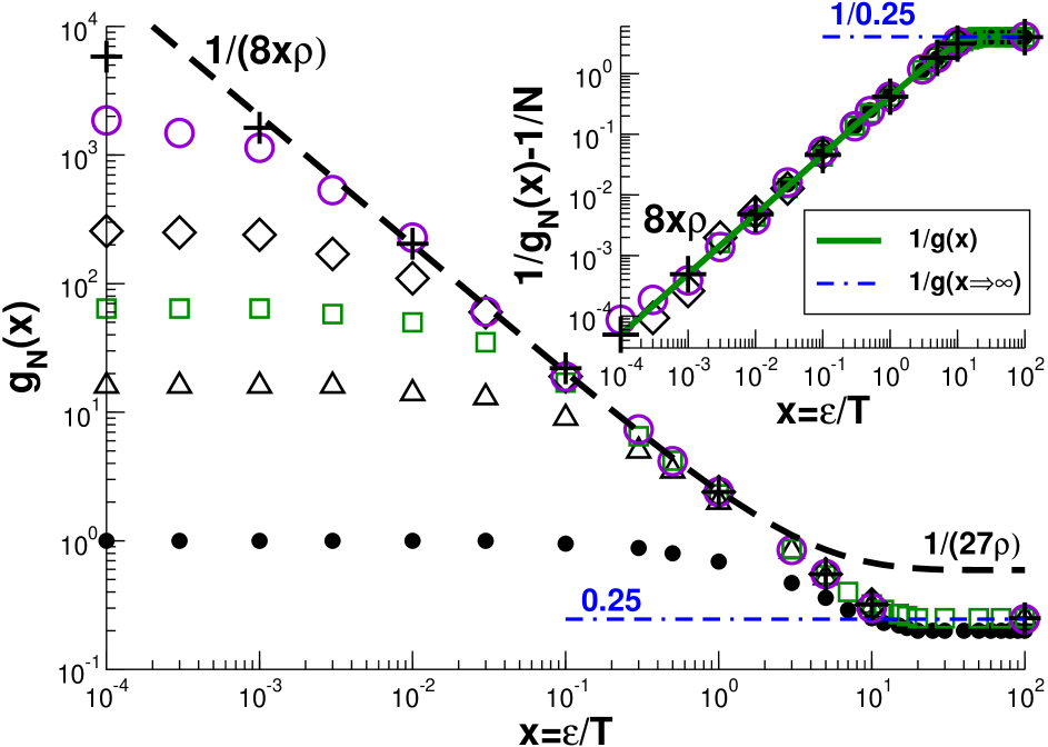
The key control property characterizing the decree of coupling of the polymer chains due to the imposed penalty is the dimensionless compressibility of asymptotically long chains. As suggested by Eq. (43), we compute first the dimensionless compressibility from the low- limit of the total monomer structure factor for different overlap penalties and chain lengths (see below for details). These raw data are presented in Fig. 14 as a function of . As one expects, decreases monotonously with . Note that the structure factor measures the complete compressibility, not just its excess contribution. As can be seen, e.g., from Eq. (69) or from the virial expansion of polymer solutions DegennesBook , the compressibility can be written in general as
| (98) |
for all with being the excess contribution to the compressibility which may, at least in principle, depend on .535353Small corrections may arise as they do arise for the chemical potential as shown below in Sec. 4.6. As can be seen from the inset of Fig. 14, all rescaled compressibilities collapse, however, on one -independent master curve if one plots as a function of , even the compressibilities obtained for unconnected beads (). Within numerical accuracy the -dependence observed for can therefore be attributed to the trivial osmotic contribution and the excess compressibility is thus identical to the compressibility of asymptotically long chains. The bold line indicated in the inset presents the best values of summarized in Table 1. These values have been obtained from the excess compressibilities for the largest chain length available for . A precise numerical determination of becomes impossible for even smaller overlap penalties. We thus have used for the smallest -values sampled the theoretical prediction
| (99) |
for due to the postulated free energy, Eq. (69). The prefactor representing the bare monomer interaction is indicated by the dashed line in the main panel of Fig. 14. Hence, for weak interactions. The underlined term is the leading correction due to the density fluctuation contribution to the free energy. It implies that the excess compressibilities for polymer melts and unconnected beads cannot be completely identical. However, the difference is far too small to be measurable in the limit where Eq. (99) applies. Although this result is unfortunate from the theoretical point of view, the data collapse observed in the inset suggests that it is acceptable to numerically estimate the long chain compressibility by computing the structure factors of rather short chains.


We now turn to the total structure factor shown in Fig. 15 to explain how the compressibilities have been obtained. Only chains of length are presented for clarity. Since the wavevectors used for computing must be commensurate with the cubic simulation box of linear dimension , i.e. the smallest possible wavevector is , it thus is important to have a sufficiently large box for a reasonable determination of . Note that around and above monomer structure and lattice effects become important. Being interested in universal physical behavior we focus on wavevectors . For comparison, we have also included the single chain form factor for (bold line). Note that the qualitative shape of — decaying monotonously with from its maximum value — depends very little on the overlap penalty (not shown). We remind that the “random phase approximation” (RPA) formula DegennesBook ; DoiEdwardsBook
| (100) |
relates the total structure factor to the measured form factor. Eq. (100) is of course consistent with Eq. (98) in the limit. It allows to directly fit for the excess compressibility using the measured structure factor and form factor , at least in the -range where the RPA approximation applies. As may be seen from the figure, indeed decreases systematically with , i.e. with decreasing . For it also decays monotonously with , again in agreement with Eq. (100). Interestingly, this becomes qualitatively different for larger excluded volume interactions () where the total structure factor is essentially constant (in double-logarithmic coordinates), very weakly increasing monotonously with . The RPA formula apparently does not apply in this limit in agreement with Eq. (48). Fortunately, this is of no concern for our main purpose — to compute — since in precisely this limit the compressibility is readily obtained from a broad plateau (even for much smaller boxes) which in addition becomes chain length independent, as we have already seen from the inset of Fiq. (14). Using boxes with it is possible to directly measure the plateau values for . For smaller we have simulated boxes with containing monomers and corresponding to a smallest wavevector . This box size becomes again insufficient for the smallest reduced overlap penalties we have simulated, as shown in Fig. 15 for (dashed line). It is for these values where the RPA formula, Eq. (100), allowing to fit the deviation from the (barely visible) plateau, has been particulary useful.
As already stated in Sec. 2.3, for intermediate wavevectors (where corresponds to distances much smaller than the radius of gyration and much larger than the monomer size) the general RPA Eq. (100) may be rewritten as
| (101) |
where we have used that the form factor becomes DoiEdwardsBook . This assumes that corrections to Gaussian chain statistics may be ignored WBJSOMB07 ; BJSOBW07 and that finite chain size effects are negligible. From the numerical point of view the approximated RPA Eq. (101) has the disadvantage that the effective bond length needs to be determined first. As shown in Fig. 16, it has the advantage that it allows for an additional test of the values of and indicated in Table 1. The main panel presents the rescaled structure factor for chains of length as a function of with being obtained from using Eq. (44). All data collapse on the master curve indicated by the bold line provided that the wavevector remains sufficiently small and no local physics is probed. That the used compressibilities are accurate is emphasized further in the inset where is plotted as a function of using only sufficiently small wavevectors . According to Eq. (101) all data should collapse on the bisection line in double-logarithmic coordinates if the correct compressibilities are used. This is indeed the case. Please note the weak deviations visible for which is due to the breakdown of the RPA formula for large mentioned above.
4.5 Chemical potential: Gaussian contribution
According to Flory’s ideality hypothesis the chemical potential of polymer melts is expected to be extensive with respect to their mass DegennesBook . Fig. 17 presents the reduced excess contribution to the chemical potential, , obtained using thermodynamic integration (as explained below) for three chain lengths , , and as functions of . As one expects, increases first linearly with and then levels off. Chain length effects are again small on the logarithmic scale chosen in the plot. For large the chemical potential becomes slightly larger for beads () than for long chains where as shown by the dash-dotted line. That the chemical potential of polymer chains is reduced compared to unconnected beads is expected due to the (effectively) attractive bond potential. For this reduction should be described by the density fluctuation contribution to the free energy [Eq. (69)] which corresponds to an excess chemical potential
| (102) | |||||
for with being the second virial of unconnected beads. The dashed line in Fig. 17 presents the leading contribution for unconnected beads, the bold line in addition the underlined connectivity contribution in Eq. (102). Surprisingly, it turns out that the simple second virial approximation provides a better fit over the entire -range than the full prediction. That the density fluctuation contribution overestimates the reduction of the chemical potential for is in agreement with Eq. (48). For where Eq. (102) applies in principle the relative correction, scaling as , becomes unfortunately too small to allow a fair test of the theory using the measured chemical potential.

We now explain how the chemical potential presented in Fig. 17 has been obtained. Obviously, the simple insertion method due to Widom FrenkelSmitBook becomes rapidly inefficient with increasing . Generalizing the method suggested in MP94 ; WM94 we have performed the thermodynamic integration FrenkelSmitBook
| (103) |
over discrete values of the affinity characterizing the excluded volume interaction of a ghost (g) chain that is inserted into an equilibrated system (s). refers to the mean number of lattice sites where system and ghost monomer cube corners overlap at a given interaction . Generalizing the Potts spin mapping, Eq. (91), of the excluded volume interactions for homopolymers presented above, we use now two spin lattices, describing (as before) the interaction of the system monomers and the ghost chain. The spin lattices are kept at the same temperature and are both characterized by the same penalty which has to be paid for a complete overlap of two system monomers or two ghost monomers. The interaction of both spins is described by
| (104) |
with coupling constants defined as in Eq. (92) taken apart the energy parameter which is replaced by the tunable interaction energy . Starting with decoupled system and ghost configurations at , i.e. , we increase the interaction parameter up to , i.e. , always keeping the coupled system at equilibrium. Monitoring the distribution of the number of overlaps between system and ghost cube corners we use multihistogram methods as described in MP94 ; WM94 to improve the precision of the integral. The mean overlap number is shown in the inset of Fig. 17 as a function of for and two inverse temperatures and . Starting from the overlap number decreases monotonously with increasing coupling between system and ghost monomers. Interestingly, a power-law behavior
| (105) |
is found empirically for large (dashed line). Fitting this power law and integrating then analytically Eq. (103) provides a useful crosscheck of the numerical integration using the multihistogram analysis. This is a technically important finding, since the multihistogram analysis requires overlapping distributions of and hence much more equilibrated intermediate values as indicated for .
4.6 Chemical potential: Non-extensive corrections
4.6.1 Theoretical predictions
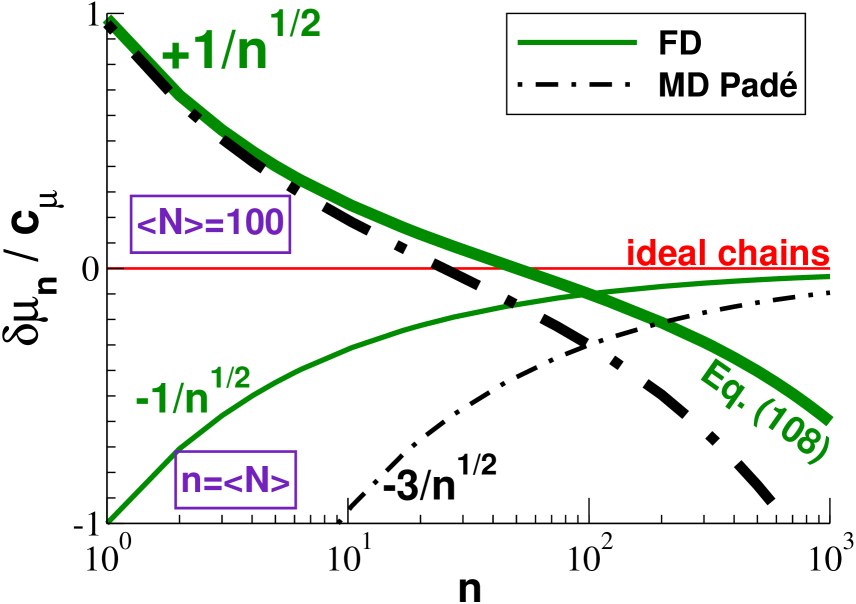
We have seen in Sec. 4.5 that the chemical potential of a test chain of length plugged into a melt of chemically identical monodisperse polymers of the same length increases essentially linearly with . Focusing now on classical BFM systems where and setting temperature to unity (), we show how small non-linear deviations may be captured numerically WJC10 . More generally, the challenge is to characterize the chemical potential of a test chain of length immersed into a bath of -chains of an arbitrary (normalized) length distribution . We remind that according to Flory’s ideality hypothesis one expects DegennesBook ,
| (106) |
with being the effective chemical potential per monomer. The upper boundary indicated in Eq. (106) is due to the well-known swelling of extremely large test chains where the bath acts as a good solution DegennesBook ; SchaferBook . As we have pointed out in Sec. 1.5, Flory’s hypothesis has been challenged by the discovery of long-range correlations imposed by the incompressibility constraint. These correlations lead to the systematic swelling of chain segments as further discussed in Sec. 5 WMBJOMMS04 ; WCK09 . We question here the validity of Flory’s hypothesis for an important thermodynamic property, the chemical potential of a test chain inserted into a three-dimensional melt. One expects that the correlation hole potential (Fig. 3) leads to a deviation
| (107) |
that is non-extensive in chain length and this irrespective of the distribution of the bath. Assuming a quenched Flory-size distribution, Eq. (20), it can be demonstrated as shown in Appendix B.6 that
| (108) |
where we have set using the swelling coefficient defined in the Sec. 1.5. Eq. (108) is represented by the bold solid line in Fig. 18. (A corresponding prediction for a monodisperse bath WJC10 is indicated by the dash-dotted line.) As anticipated by Eq. (107), the first term in Eq. (108) dominates for short test chains. The second term dominates for large test chains with becoming non-perturbative for . Both contributions to decrease with increasing .545454This corresponds to an effective enhancement factor of the partition function quite similar to the in the standard excluded volume statistics with being the self-avoiding walk susceptibility exponent DegennesBook . Interestingly, while decreases at fixed , it increases as (thin solid line) for a test chain with . The chemical potential of typical chains of the bath approaches thus the ideal chain limit from below.
Flory-distributed polymer melts are obtained naturally in systems of self-assembled linear EP where branching and the formation of closed rings are forbidden CC90 . Since the suggested correction, Eq. (108), to the ideal chain chemical potential is weak, the system must remain to leading order Flory distributed and Eq. (108) should thus hold.555555The chemical potential of a test chain does depend on the length distribution of the bath. However, for an infinite macroscopically homogeneous systems it is independent on whether this distribution is annealed or quenched, i.e. if it is allowed to fluctuate or not. This follows from the well-known behavior of fluctuations of extensive parameters in macroscopic systems: the relative fluctuations vanish as as the total volume . The latter limit is taken first in our calculations, i.e. we consider an infinite number of (annealed or quenched) chains. The large- limit is then taken afterwards. This correction implies for the annealed length distribution of linear EP that (to leading order)
| (109) | |||||
| (110) |
where both the lower () and the upper limit () of validity are irrelevant in the large- limit. Note that Eq. (110) is properly normalized, i.e. the prefactor of the distribution remains exact if is given by Eq. (108). At given the first moment increases slightly
| (111) |
and, more generally, one expects for the th moment
| (112) |
with being the Gamma function abramowitz . The non-exponentiality parameter thus scales as
| (113) |
being a -dependent geometrical factor.565656The polydispersity index , i.e. the ratio of weight average and number average, becomes . In this sense, the distribution becomes narrower just as for dilute good solvent EP where WMC98b ; Yeruk77 .
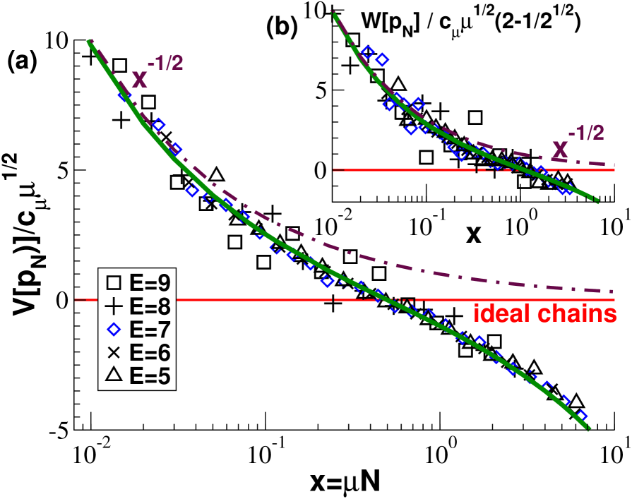
4.6.2 Computational results for EP melts
Eq. (110) and Eq. (113) allow us to demonstrate numerically the prediction, Eq. (108), from the observed non-exponentiality of the length distribution of EP melts obtained as described in Sec. 3.5. As demonstrated in the main panel of Fig. 10 these EP melts are indeed essentially Flory distributed, i.e. the length distribution decays to leading order exponentially with the reduced chain length . However, deviations for are visible in Fig. 10(c) in qualitative agreement with the predicted positive deviation of the chemical potential, Eq. (107). The curvature of is further analyzed in Fig. 19. Motivated by Eq. (109), we present in panel (a) the functional
| (114) |
where the second term takes off the ideal contribution to the chemical potential. The last term is due to the normalization of and eliminates a trivial vertical shift depending on the scission energy . Consistently with Eq. (111), the chemical potential per monomer has been obtained from the measured mean chain length using
| (115) |
Note that and become numerically indistinguishable for . If the Gaussian contribution to the chemical potential is properly subtracted one expects to obtain directly the non-Gaussian deviation to the chemical potential, . Due to Eq. (108) the functional should thus scale as
| (116) |
with as indicated by the bold line in the panel. This is well born out by the data collapse obtained up to . Obviously, the statistics deteriorates for for all energies due to the exponential cutoff of . Unfortunately, the statistics of the length histograms decreases strongly with and becomes too low for a meaningful comparison for . It is for this numerical reason that we use Eq. (115) rather than the large- limit since this allows us to add the two histograms for and for which high precision data is available. Otherwise these energies would deviate from Eq. (116) for large due to an insufficient subtraction of the leading Gaussian contribution.
Since the subtraction of the large linear Gaussian contribution is in any case a delicate issue we present in panel (b) of Fig. 19 a second functional,
| (117) |
where by construction this contribution is eliminated following a suggestion made recently by Semenov and Johner ANS03 . The normalization factor appearing in Eq. (117) eliminates again a weak vertical scission energy dependence of the data. Obviously, for perfectly Flory-distributed chains. Following Eq. (108) and Eq. (109) one expects
| (118) |
with . Eq. (118) is indicated by the bold line which compares again rather well with the presented data.
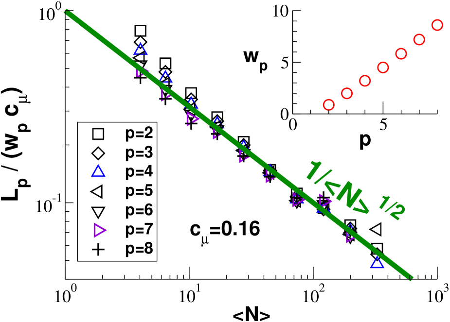
The functionals presented in Fig. 19 require high-accuracy histograms. That is only approximately Flory distributed can be more readily seen using the “non-exponentiality parameter” . Obviously, for rigorously Gaussian chains. As stated in Eq. (113), we expect the non-exponentiality parameter to decay as , i.e. as the correlation hole potential of the typical melt chain. The main panel of Fig. 20 presents as a function of . The predicted power-law decay is clearly demonstrated by the data. Note that the scaling of the vertical axis with the -dependent geometrical factors allows to bring all moments on the same master curve. As can be seen from the inset of Fig. 20, this scaling is significant since varies over nearly a decade. Deviations from the predicted scaling are visible, not surprisingly, for small . Since the coefficient is known the data collapse on the theoretical prediction (bold line) has been produced without any free adjustable parameter.
4.7 Summary
In this section we have discussed various thermodynamic properties of BFM melts at our reference volume fraction . For large overlap penalties all thermodynamic properties remain similar to the known values for athermal BFM systems () MP94 ; WM94 ; WBM07 . From the computational point of view this is of some interest since it suggests the equilibration and sampling of configurations at a reasonable cost at overlap penalties between and where the slithering snake algorithm is still efficient. Decreasing the monomer interaction further we have found, as one expects, good agreement with the prediction by Edwards, Eq. (69), for small overlap penalties (). In this limit the thermodynamics is essentially determined by the second virial contribution, Eq. (89). Interestingly, being the second derivative of the free energy with respect to the inverse temperature the specific heat allows the verification of the predicted scaling of the free energy contribution due to the chain connectivity (Fig. 13). The central control parameter of this work, the dimensionless compressibility , is discussed in Sec. 4.4. While the determination of is numerically trivial for large overlap penalties, more care is needed for (Fig. 14). Note that the static RPA, Eq. (45), breaks down in the opposite limit () where the structure factors of beads and polymer melts become ultimately identical, .
For a test chain of length immersed into a bath of monodisperse chains of length we have confirmed by thermodynamic integration in Sec. 4.5 that the chemical potential is essentially extensive with respect to the chain length, as expected from Flory’s ideality hypothesis. In order to demonstrate that the small deviations predicted by the perturbation theory WJC10 exist, we have investigated in Sec. 4.6 essentially Flory-distributed (Fig. 10) self-assembled EP systems. The detailed analysis of the measured length distribution (Fig. 19) has allowed us to show the existence of a correction , Eq. (108), scaling essentially as the correlation hole penalty for . The observed deviations for EP systems WJC10 beg for an improved numerical verification by means of the thermodynamic integration method (Sec. 4.5) for test chains immersed into monodisperse melts.575757The presented results for dense polymer solutions may also be of relevance to the chemical potential of dilute polymer chains at and around the -point which has received attention recently Rubinstein08 ; SNM09 . The reason for this connection is that (taken apart different prefactors) the same effective interaction potential enters the perturbation calculation in the low wavevector limit. A non-extensive correction in three dimensions is thus to be expected.
5 Intramolecular conformational properties
5.1 Introduction
We turn now to the description of intrachain conformational properties of BFM melts at volume fraction and temperature comparing our numerical results to the theoretical predictions announced in Sec. 1.5 and Sec. 2. We discuss first the properties on monomeric level (Sec. 5.2) and show then how the effective bond length for asymptotically long chains can be obtained using the theoretical input developed in Sec. 2. We present then the bond-bond correlation function as a function of curvilinear distance (Sec. 5.4.1) and as a function of the spatial distance between both bonds (Sec. 5.4.2). Higher moments of the distribution and its deviations from Flory’s ideality hypothesis will be analyzed in Sec. 5.5 and Sec. 5.6, respectively. We turn finally to the characterization of an experimental relevant observable, the intramolecular form factor .
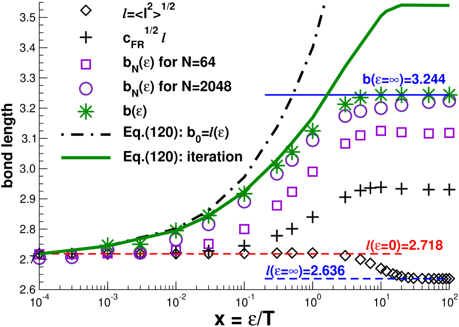
5.2 Bond properties
We begin by characterizing local-scale features of the algorithm described in Sec. 3. By definition of our version of the BFM algorithm the bond length is allowed to fluctuate between and . One expects that switching on the overlap penalty will suppress large bonds due to the increasing pressure. The mean bond length is characterized by the root-mean-square length . (Other moments yield similar results.) The mean bond length rapidly becomes () chain length independent Paul91a . As can be seen from Fig. 21, shows a monotonous decay between and . As other local properties, the bond length becomes constant in the small- and large- limits (dashed lines). The value gives the lower bound for the effective bond length of asymptotically long chains (stars) obtained below.
Defining the bond angle between two subsequent bonds by the scalar product of the normalized bond vectors , the local chain rigidity may be characterized by and . Note that and can be regarded as chain length independent, just as the mean bond length. The local rigidity is negligible for , i.e. and due to the symmetry of the distribution with respect to . The rigidity then increases around and becomes constant again for large where and WCK09 . The increase of the local rigidity for larger excluded volume interactions is of course expected due to the suppression of immediate backfoldings corresponding to bond angles WPB92 . The distribution therefore becomes lopsided towards smaller (not shown). According to Eq. (18) the effective bond length of a “freely rotating” (FR) chain is given by with . This simple model, indicated by the crosses in Fig. 21, yields a qualitatively reasonable trend (monotonous increase of the effective bond length at ) but fails to fit the directly measured effective bond lengths quantitatively WCK09 .
5.3 Mean-squared chain and subchain size
5.3.1 Total chain size
One way to characterize the total chain size is to measure the second moment of the chain end-to-end distance . We consider the ratio to compare the measured chain size with the ideal chain behavior which is commonly taken as granted DegennesBook ; DoiEdwardsBook ; Flory49 and which is the basis of our perturbation calculation (Sec. 2.4). The task is to extrapolate for the effective bond length of asymptotically long chains. The ratio for and and the asymptotic limit — obtained by extrapolation as described below — are presented in Fig. 21. Obviously, for all in the small- limit. increases then in the intermediate -window before it levels off at . The swelling due to the excluded volume interaction is the stronger the larger the chain length, i.e. increases monotonously with . This swelling thus cannot be attributed to a local rigidity as described, e.g., by the freely-rotating chain model.
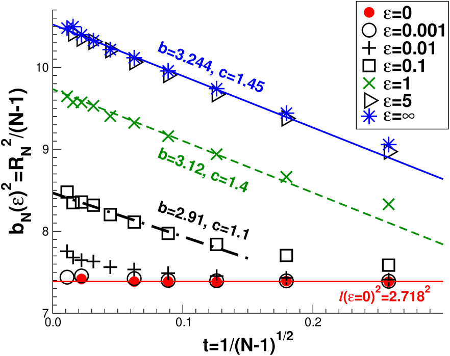
The -effect can be seen better in Fig. 22 where we have plotted for several penalties as a function of . The choice of the horizontal axis is motivated by Eq. (10) suggesting the linear relation
| (119) |
with being the swelling coefficient defined in Sec. 1.5 and an additional numerical prefactor of order unity. This prefactor has been introduced in agreement with Eq. (86). The reason for this coefficient is that the corrections to Gaussian behavior differ slightly for internal chain segments [as described by Eq. (10)] and the total chain size which is characterized in Fig. 22. We remind that for . However, since this value corresponds to the limit of a very slowly converging integral WBM07 it is better to use Eq. (119) as a two-parameter fit for and and to crosscheck then whether the fitted is of order unity. As shown in the figure for three overlap penalties, this method can be used reasonably for overlap penalties as low as , albeit with decreasing it systematically underestimates the “true” -values indicated in Table 1. Please note that for and . Chains with would be required to use this method for even smaller . In this limit it is better to use as a first step the value of the largest chain length simulated as a (rather reasonable) lower bound for .
5.3.2 Subchain size
The mean-squared subchain size is presented in Figs. 23 and 24 where we focus on melts without monomer overlap () WBM07 . We show how the effective bond length for asymptotically long chains may be extrapolated from the measured for finite arc-length and finite chain length using the perturbation prediction Eq. (10).
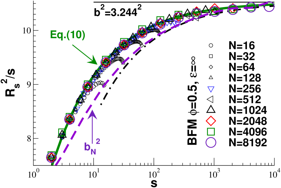
As already remarked by Auhl et al. Auhl03 , Fig. 23 shows clearly that the chains are swollen, i.e. increases systematically and this up to very large arc-length . In agreement with Eq. (10), the Gaussian behavior (horizontal line) is approached from below and the deviation decays as . The indicated bold line corresponds to and which fits nicely the data over several decades in — provided that chain end effects can be neglected (). Note that a systematic underestimation of the true effective bond length would be obtained by taking the largest value available, say, for monodisperse chains of length . Interestingly, does not approach the asymptotic limit monotonically Auhl03 ; WBM07 . Especially for short chains one finds a non-monotonic behavior for . This means that the total chain end-to-end distance shows even more pronounced deviations from the asymptotic limit. We emphasize that the non-monotonicity of becomes weaker with increasing and that, as one expects, the inner distances, as well as the total chain size, are characterized by the same effective bond length for large or .585858We note en passant that this is not the case for the compact chain conformations adopted by chains in strictly 2D melts where the effective bond length associated to the chain ends is smaller than the one for subchains even for MWK10 . The non-monotonic behavior may be qualitatively understood by the reduced self-interactions at the chain ends which lessens the swelling on these scales. Our perturbation prediction Eq. (86) is indicated in Fig. 23 by the dash-dotted line. As already remarked, this prediction contains a slowly converging numerical integral of order unity. The dash-dotted line corresponds to the value predicted for asymptotically long chains, the dashed line to the slightly smaller value fitted in Fig. 22. In summary, it is clear that one should use the subchain size rather than the total chain size to obtain in a computational study a reliable fit of the effective bond length .

The representation chosen in Fig. 23 is not the most convenient one for an accurate determination of and . How precise coefficients may be obtained according to Eq. (10) is addressed in the Fig. 24 for chains of length . In a first step should be plotted as a function of just as in Fig. 22. This allows for a first rough estimation of . Since data for large are less visible in this representation, we recommend for the fine-tuning of to switch then to logarithmic coordinates with a vertical axis for different trial values of . The correct value of is found by adjusting the axes such that extrapolates linearly as a function of to zero for large .595959For the bead-spring model presented in Ref. WBM07 the empirical swelling coefficient is shown to differ for yet unknown reasons by a few percents from the predicted value . We assume for the fine-tuning that higher order perturbation corrections may be neglected, i.e. we take Eq. (10) literally. The plot shows that this method is very sensitive, yielding a best value for that agrees with the theory over more than one order of magnitude without curvature. Using this method we have determined the effective bond lengths for a broad range of overlap penalties as indicated in Table 1 and shown by the stars in Fig. 21 WCK09 .
5.3.3 Predicting the effective bond length
Up to now, we have used the theoretical results to fit the effective bond length , rather than to predict it from the known thermodynamic properties and local model features such as the bond length . As reminded in Eq. (72) the increase of the effective bond length for weakly interacting and asymptotically long polymer melts has been in fact calculated long ago by Edwards DoiEdwardsBook . Following a suggestion made by Muthukumar and Edwards Edwards82 this perturbation result may be rewritten as a recursion relation
| (120) |
with being the bond length after the -th iteration step, the measured dimensionless compressibility and the relevant Ginzburg parameter quantifying the strength of the interaction acting on a chain segment of length . Since becomes small for large compressibilities , one expects good agreement with our data for small . If we set this yields after one iteration () the dash-dotted line indicated in Fig. 21, i.e. a reasonable prediction is only achieved up to . The predictive power of Eq. (120) can be considerably improved over nearly two decades up to if one applies the formula iteratively using the effective bond length obtained at step as input for the Ginzburg parameter for computing . This recursion converges rapidly as shown by the bold line indicated in Fig. 21 obtained after 20 iterations.606060Essentially the same result is obtained up to if one sets directly using the measured effective bond length as start value of the iteration. Note that for where Eq. (120) fits our data nicely. The fix-point solution of Eq. (120) does not capture correctly the leveling off of setting in above . Since the Ginzburg parameter becomes there of order one, this is to be expected. In summary, we have shown that the iteration of Eq. (120) allows a good prediction for for . If reliable values for compressibilities are available, this is the method of choice if one cannot afford to simulate very long chains.
5.4 Bond-bond correlation function
5.4.1 Bond-bond correlation function
As we have seen in Fig. 24, to demonstrate the deviations from Flory’s ideality hypothesis starting from the subchain size requires to subtract a large Gaussian contribution . Unfortunately, this requires as a first step the precise determination of the effective bond length for asymptotically long chains which might not be available. Indeed we have used in the preceding Sec. 5.3.2 the fact that the scaling of critically depends on this accurate value to improve the estimation of . Hence, it would be nice to demonstrate directly the scaling implied by our key prediction without any tunable parameter. The trick to achieve this is similar to our demonstration of the density fluctuation contributions to the free energy, Eq. (69), presented in Sec. 4.3: We consider the curvature of , i.e. its second derivative with respect to . Using Eq. (4) this second derivative is obtained directly from the bond-bond correlation function computed by averaging over all pairs of monomers . We remind that is generally believed to decrease exponentially as in Eq. (15). This textbook belief is based on the assumption that all long range interactions are negligible on distances larger than . Hence, only correlations along the backbone of the chains should matter and it is then straightforward to work out that an exponential cutoff is inevitable due to the multiplicative loss of any information transferred recursively along the chain FloryBook .
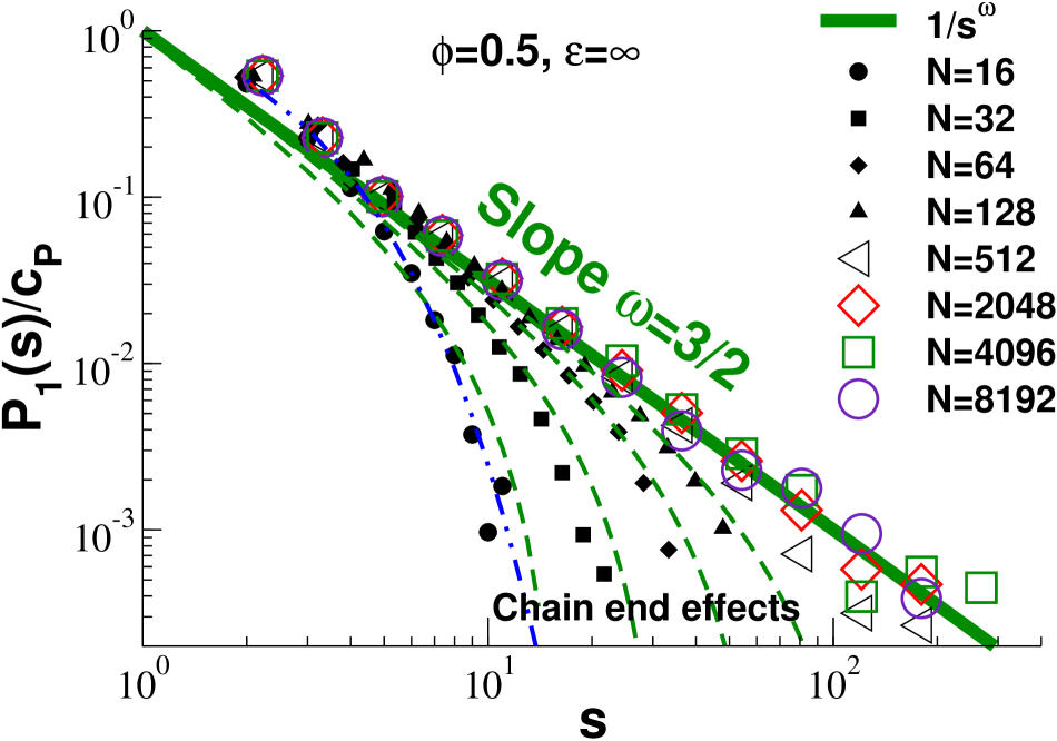
The bond-bond correlation function obtained for monodisperse chains at and is presented in Fig. 25. The power-law decay with exponent predicted by our key perturbation result Eq. (9) is perfectly confirmed by the larger chains (). As can be seen for , exponentials are compatible with the data of short chains, however. This might explain why the power-law scaling has been overlooked in older numerical studies, since good statistics for large chains () has only become available recently. However, it is clearly shown that approaches systematically the scale-free asymptote with increasing . The departure from this limit is fully accounted for by the theory if chain end effects are carefully considered (dashed lines). Generalizing Eq. (9) using the Padé approximation, Eq. (63), perturbation theory yields
| (121) |
where we have set WBM07 . For this is consistent with Eq. (9). In the limit of large , the correlation functions vanish rigorously as . Considering that non-universal features cannot be neglected for short chain properties and that the theory does not allow for any free fitting parameter, the agreement found in Fig. 25 is rather satisfactory.
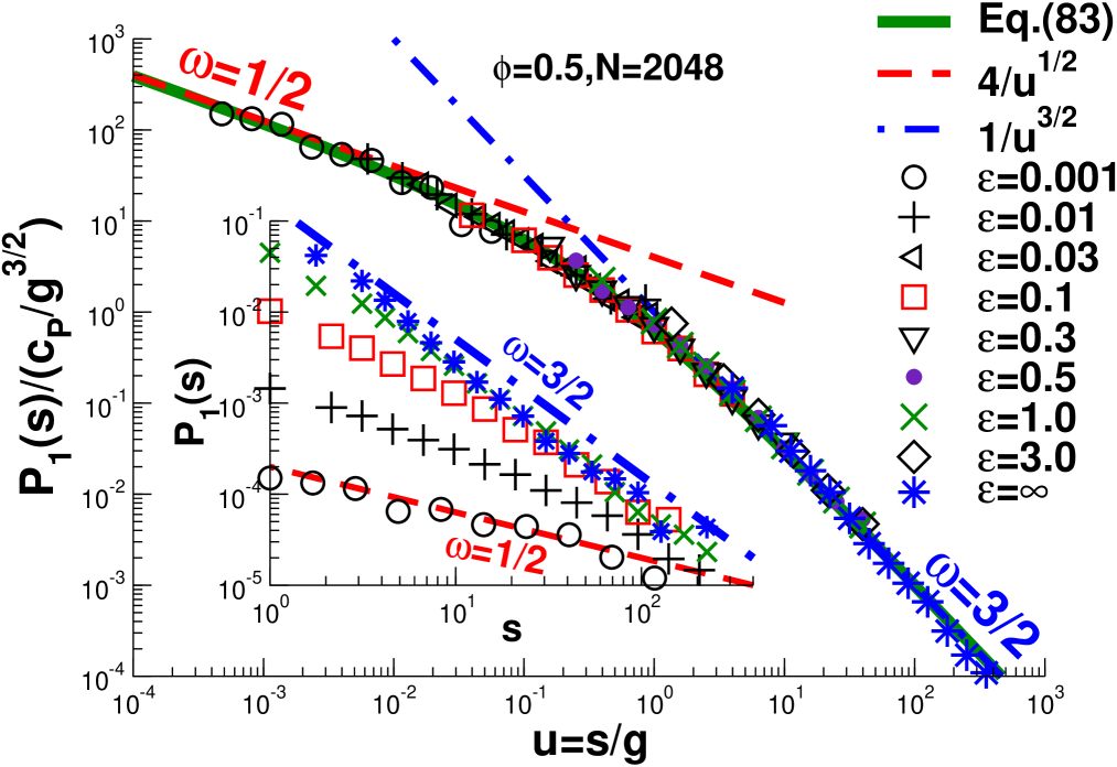
The bond-bond correlation function for different overlap penalties is presented in Fig. 26 for chains of length WCK09 . As can be seen from the unscaled data shown in the inset, approaches a power law with exponent (dashed line) in the limit of weak overlap penalties in agreement with Eq. (84). For our data is compatible with an exponent (dash-dotted line) as suggested by Eq. (9). Hence, we have demonstrated without any tunable parameter that Flory’s ideality hypothesis is systematically violated for all segment lengths and all overlap penalties . As suggested by Eq. (83), the main panel of Fig. 26 presents as a function of the reduced arc-length using the dimensionless compressibilities and effective bond lengths from Table 1. The data collapse is remarkable as long as . The relation Eq. (83) is indicated by the bold line; it is in perfect agreement with the simulation data.616161Eq. (83) has also been applied successfully to the obtained from single-chain-in-mean-field simulation MMuller06 . The asymptotical behavior with for and for is shown by the dashed and dash-dotted lines, respectively. As predicted by Eq. (9), one recovers the power law irrespective of the blob size . This suggests that the exponent is not due to local physics on the monomer scale, since for distances much larger than the monomer or even the thermal blob are probed.
5.4.2 Distance dependence of angular correlations
We have seen in the previous paragraph that decays for as a power law with an exponent . Since the decay of resembles the return probability of a random walk , it is tempting Rubinstein08 to attribute the observed effect to “local self-kicks” at a distance involving the bonds and themselves (or their immediate neighbors). Accordingly, the bond-bond correlation function should reveal a -correlation if sampled as a function of the distance between bond pairs. This interpretation turns out to be incorrect, however, and we will show that the power law in simply translates as WJO10
| (122) |
As demonstrated analytically in Sec. B.5, one expects indeed for incompressible solutions of infinite chains that
| (123) |
as suggested by Eq. (122), i.e. the angular correlations are genuinely long-ranged. As discussed in Sec. B.5.4 the upper cutoff arises due to the enhanced weight of stretched chain segments which align bond pairs for distances . Unfortunately, this cutoff increases rather slowly with chain length WJO10
| (124) |
The simulation of computationally challenging chain lengths thus is required to demonstrate numerically the predicted power-law decay of . Generalizing Eq. (123) for Flory-distributed EP one obtains according to Eq. (219) that
| (125) |
with being a scaling function of and a phenomenological constant set (in practice) by the finite local chain rigidity. The angular correlation function for EP systems is thus predicted to level off for large reduced distances.626262For monodisperse systems one finds instead for very large distances with due to the increasing contribution of stretched bonds WJO10 .
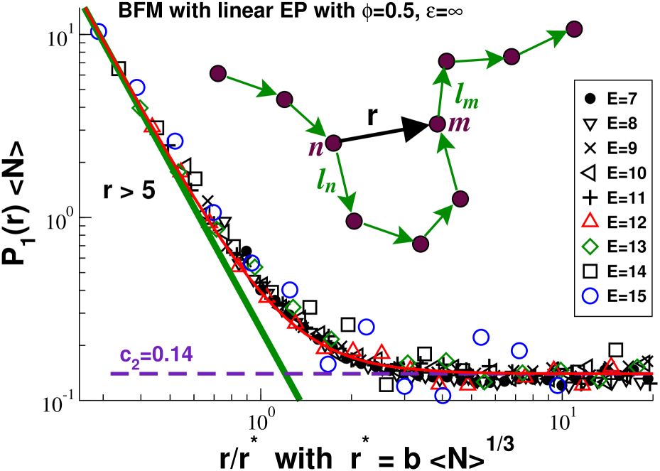
We present in Fig. 27 numerical results obtained for systems containing Flory-distributed EP. As indicated in the sketch, is obtained by averaging of all intrachain bond pairs of same distance . To avoid trivial correlations the second bond is outside the subchain between the monomer and defining the vector WJO10 ; ANS10a . Model-depending physics not taken into account by theory obviously becomes relevant for short distances corresponding to subchains of a couple of monomers. For clarity, we have thus omitted data points with . For small distance the (unscaled) bond-bond correlation function is found to decay strongly as expected from Eq. (125). Note that in this limit does neither depend on the mean chain length nor the chain length distribution, i.e. the same behavior is observed for monodisperse chains. See Ref. WJO10 for details. To scale away the -dependence in the large- limit, we trace in Fig. 27 the rescaled bond-bond correlation function as a function of with using the mean chain lengths indicated in Table 3. Note that the error bars (not shown) become clearly much larger than the symbol size for large bond energies . It is fair to state, however, that all data points collapse nicely on the one master curve indicated by the thin line predicted by Eq. (125). The asymptotic power law Eq. (123) is indicated by the bold line. That for EP becomes constant for confirms a non-trivial prediction of the theory.636363The clearly visible plateau can be used to determine the coefficient . The same coefficient can then be used for fitting the large- behavior of monodisperse systems. Note that the best fit value is close to , the independently determined bond-bond correlation between adjacent bond vectors.
5.5 Higher moments

The preceding discussion focused on the second moment of the subchain size distribution and its derivatives with respect to . We have also computed higher moments with WBM07 . (For clarity we focus here on monodisperse chains.) We compare these moments in Fig. 28 with Eq. (77) tracing the cummulant defined in Eq. (26) as a function of
| (126) |
All data sets collapse nicely on the prediction (bold line) for small .646464The curvature of the data at small is due to the finite extensibility of the subchains which becomes more marked for higher moments. It is important that the same effective bond length is obtained from the analysis of all functions as illustrated in Fig. 28. Otherwise we would regard equilibration and statistics as insufficient.
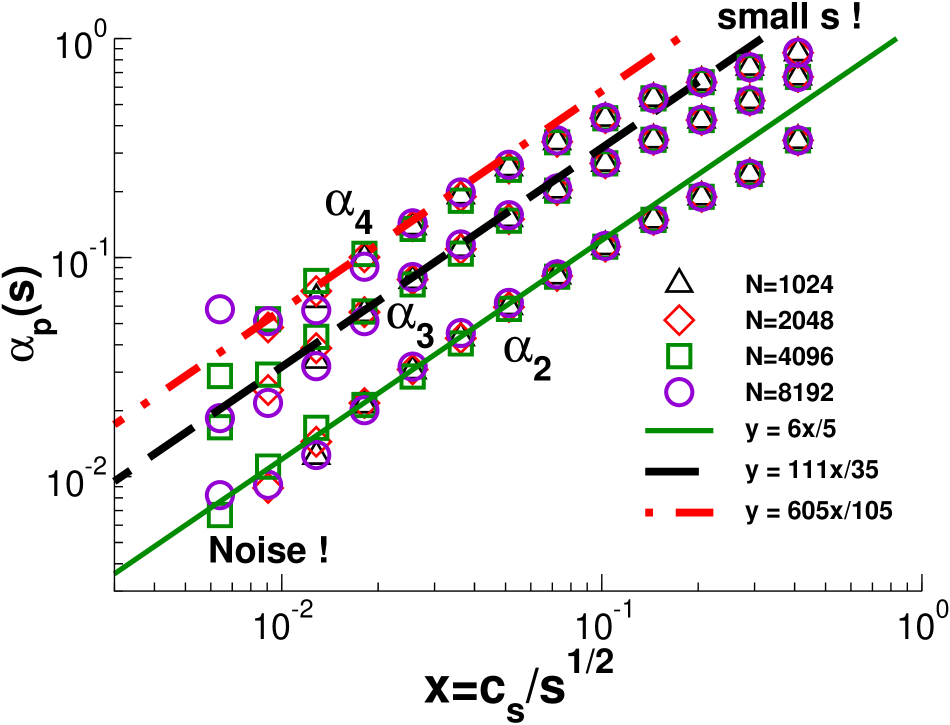
The failure of Flory’s hypothesis can also be demonstrated by means of the non-Gaussianity parameter defined in Eq. (27) which compares the -th moment with the second moment (). In contrast to the related function this has the advantage that here two measured properties are compared without any tunable parameter, such as . Fig. 29 presents vs. for three moments. For each we find perfect data collapse for all which confirms the expected linear relationship .656565If one plots as a function of the r.h.s. of Eq. (78) all data points for all moments and even for too small collapse on one master curve just as in Fig. (28). The lines indicate the theoretical prediction Eq. (78). The prefactors , and for , and respectively are nicely confirmed. They increase strongly with , i.e. the non-Gaussianity becomes more pronounced with increasing . Hence, should be best fitted by the second moment where the non-Gaussian behavior is the weakest.
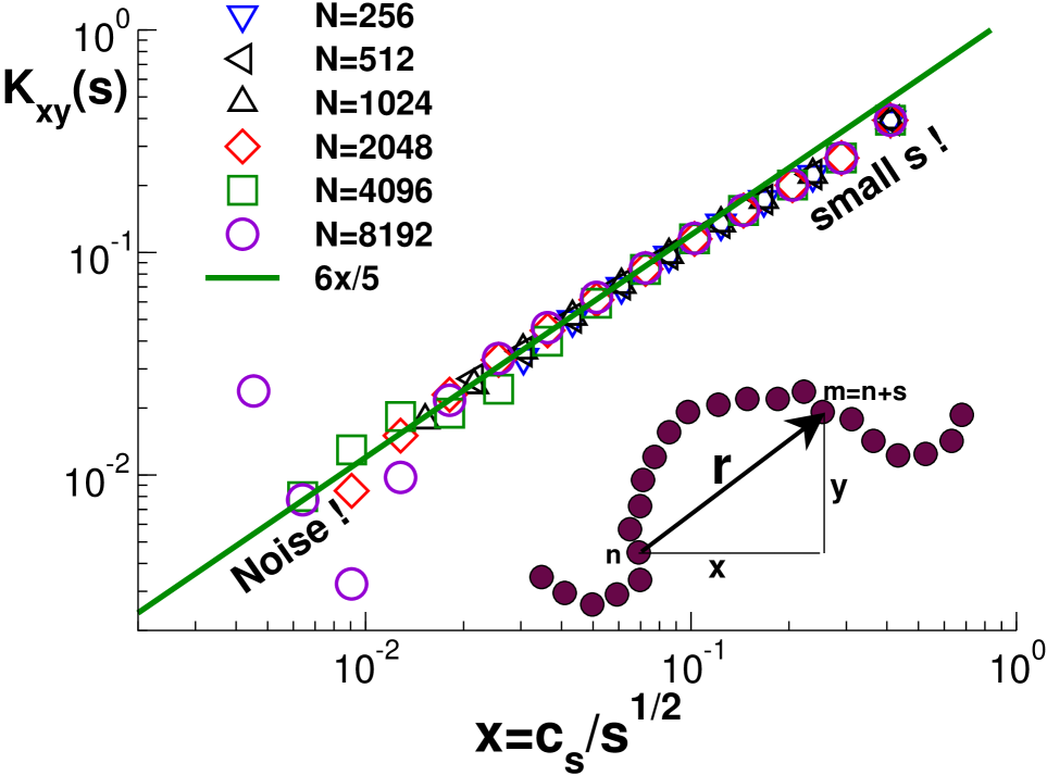
Figure 30 presents a similar correlation function which measures the non-Gaussian correlations of different spatial directions. It is defined by for the two spatial components and of the vector as illustrated by the sketch given at the bottom of Fig. 30. Symmetry allows to average over the three pairs of directions , and . Following the general scaling argument given in Sec. 2 we expect which is confirmed by the perturbation result
| (127) |
This is nicely confirmed by the linear relationship found (bold line) on which all data from both simulation models collapse perfectly. The different directions of subchains are therefore coupled. As explained at the end of Appendix B.1, and must be identical if the Fourier transformed subchain size distribution can be expanded in terms of and this irrespective of the values the expansion coefficients take. Fig. 30 confirms, hence, that our computational systems are perfectly isotropic and tests the validity of the general analytical expansion. The correlation function is of particular interest since the zero-shear viscosity should be proportional to where we assume following Edwards DoiEdwardsBook that only intrachain stresses contribute to the shear stress . Hence, our results suggest that the classical calculations DoiEdwardsBook — assuming incorrectly — should be revisited.
5.6 Corrections to the subchain size distribution
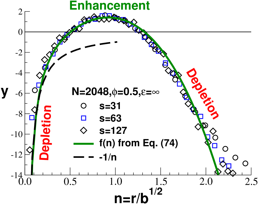
We turn finally to the subchain size distribution itself which is presented in Fig. 31. From the theoretical point of view is the most fundamental property from which all others can be derived. The normalized histograms are computed by counting the number of subchain vectors between and with being the width of the bin and one divides then by the spherical bin volume. Since the BFM model is a lattice model, this volume is not but given by the number of lattice sites the subchain vector can actually point to for being allocated to the bin. Incorrect histograms are obtained for small if this is not taken into account. Averages are taken over all (sub)chains, just as before. Clearly, non-universal physics must show up for small vector length and small curvilinear distance and we concentrate therefore on values and . When plotted in linear coordinates as in Fig. 11 of WBM07 , compares roughly with the Gaussian prediction given by Eq. (2), but presents a distinct depletion for small subchain vectors with and an enhanced regime for . To analyse the data it is better to consider instead of the relative deviation which should further be divided by the strength of the subchain correlation hole, . As presented in Fig. 31 this yields a direct test of the relation Eq. (75) derived in Appendix B.2. The figure demonstrates nicely the scaling of the data for all . It shows further a good collapse of the data close to the universal function predicted by theory (bold line). Note that the depletion scales as for small subchain vectors (dashed line). The agreement of simulation and theory is by all standards remarkable. Obviously, error bars increase strongly for where decreases strongly. The regime for very large where the finite extensibility of subchain matters has been omitted for clarity. We emphasize that this scaling plot depends very strongly on the value which is used to calculate the Gaussian reference distribution.666666As shown in Ref. WBM07 , a similar plot can be achieved which does not require a precise value of if the reduced deviation is plotted as a function of using the measured subchain size .
5.7 Intramolecular form factor
The form factor defined in Sec. 2.2.4 is an important property since it allows to make a connection between theory and simulation on the one hand and experiments of real systems on the other hand BenoitBook .

Figure 32 presents the (unscaled) form factors obtained for four different scission energies for our EP model at . The three different -regimes are indicated. Details of the length distribution matter in the Guinier regime which probes the total coil size. Non-universal contributions to the form factor arise in the “Bragg regime” at large wavevectors. Obviously, the larger the wider the intermediate Kratky regime where chain length, polydispersity and local physics do not contribute much to the deviations of the form factor from ideality. A very similar plot has been obtained for monodisperse polymers (not shown). Not surprisingly, it demonstrates that the form factors of both system classes become indistinguishable for large wavevectors. Note that the obtained for EP of different can be brought to collapse by tracing as a function of with and the measured -averaged radius of gyration as indicated in Table 3 BJSOBW07 . A similar plot can again be obtained for monodisperse chains using and .

Interestingly, a careful inspection of Fig. 32 reveals that Eq. (40) overestimates systematically the data in the Kratky regime. This can be seen more clearly in the Kratky representation given in Fig. 33 in linear coordinates.676767Such “Kratky plots” are commonly used to represent neutron scattering experiments and to test Flory’s ideality hypothesis. In applications, the existence of a Kratky plateau appears to be elusive BenoitBook . Possible causes for deviations are effects of chain stiffness and finite chain thickness. In special cases, the scattering signals from chain stiffness and thickness may compensate one another, leading fortuitously to an extended Kratky plateau Rawiso87 ; Gagliardi05 . Apparently, “Kratky plots have to be interpreted with care” BenoitBook . We present here the systems with the longest masses currently available for both monodisperse ( and ) and EP systems ( and ) BJSOBW07 . The non-monotonous behavior is in striking conflict with Flory’s hypothesis. The difference between the ideal Gaussian behavior (thin line) and the data becomes up to 20%. This difference is qualitatively expected from the perturbation theory result, Eq. (14), derived in Appendix B.3. The predicted scaling can be easily understood by means of a simple scaling relation following the discussion in Sec. 2.3.6. As the arc-length is related to the wavevector and the ideal form factor by , it follows for the difference of measured and ideal form factors that WBJSOMB07
| (128) |
which agrees with Eq. (14).686868This is the same scaling dependence which leads to for the bond-bond correlation function as a function of or as investigated in Sec. 5.4.1. The important feature of this -correction is that it depends neither on the strength of the excluded volume interaction nor on the effective bond length . Hence, it must be generally valid, even for semidilute solutions.696969It applies then for with being the semidilute blob length DegennesBook . We have checked that the result from the renormalization group theory for semidilute solutions SchaferBook ; MM00 takes the same form as Eq. (14) with an amplitude that is within of our BJSOBW07 . The prediction for infinite , Eq. (14), cannot capture the decrease of the form factor for small leading to the Guinier regime where is determined by the finite size of the simulated chains. A clearer evidence for the theory should thus be obtained by a different comparison between theory and simulation, which accounts for the finite- effects.

This is achieved in Fig. 34 which focuses on deviations for monodisperse systems with being the Debye formula. As above in our discussion of the subchain distribution and its moments one should avoid to use as Gaussian reference the ideal chain form factor expressed in terms of the effective bond length since the latter property might not be sufficiently accurate. A variation of a few percents breaks the scaling and leads to qualitatively different curves BJSOBW07 as in Fig. 24 for the moment . Since such a precision is normally not available (neither in simulation nor in experiment) it is of interest to seek for a more robust representation of the form factor deviations which does not rely on . The reference chain size is thus set in Fig. 34 by the measured radius of gyration which is used for rescaling the axis and, more importantly, to compute . (A virtually indistinguishable plot has been obtained for EP.) The scaling of the vertical axis is suggested by Eq. (14) which predicts the difference of the inverse form factors to be proportional to . Without additional parameters ( is known to high precision) we confirm the scaling of
| (129) |
as a function of with being the self-density. Importantly, our simulations allow us to verify for the fundamentally novel behavior of the master curve predicted by Eq. (14) and this over more than an order of magnitude! In this representation we do not find a change of sign for the form factor difference ( is always negative) and all regimes can be given on the same plot in logarithmic coordinates. In the Guinier regime we find now which is readily explained in terms of a standard expansion in since the first two terms in and must vanish by construction because of the definition of , Eq. (39).
5.8 Summary
In this section we have investigated various intrachain static properties of polymer melts comparing our numerical data to the predicted deviations with respect to Flory’s ideality hypothesis. From the computational side the most important point is discussed in Sec. 5.3.2 where we show how the effective bond length for asymptotically long chains should be extrapolated from subchains of finite arc-length with . That the deviations are indeed due to long-range interactions has been demonstrated from the scaling of the bond-bond correlation function in Sec. 5.4.2.
The most important finding from the experimental side concerns the scale-free deviations demonstrated for the form factor , Eq. (14). We have shown that the Kratky plot does not exhibit the plateau expected for Gaussian chains in the intermediate wavevector range. These deviations should be measurable by neutron scattering experiments of flexible chains. Unfortunately, finite persistence length effects may mask the predicted behavior if the chains are not sufficiently long. An experimental verification — e.g. following the lines of the the promising recent study Gagliardi05 — would be of great fundamental interest; it could also delineate the conditions where the predicted conformational corrections to ideality are relevant in real polymer systems and must be considered in understanding their structure, phase behavior and equilibrium dynamics. It is to the latter point we turn now our attention.
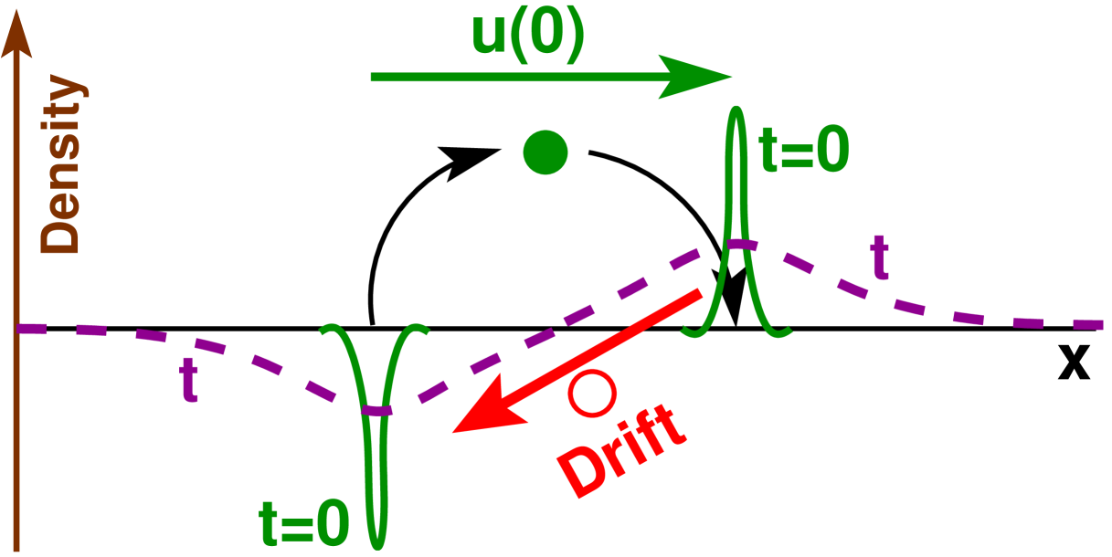
6 Scale-free dynamical correlations in polymer melts
6.1 Introduction
6.1.1 Prelude: Overdamped colloids
Dense, essentially incompressible simple liquids with conserved momentum are known to exhibit long-range correlations of the particle displacement field DhontBook ; HansenBook . As first shown in the MD simulations by Alder and Wainwright HansenBook , the coupling of displacement and momentum fields manifests itself by an algebraic decay of the VCF,
| (130) |
with being the particle velocity at time and the typical particle displacement with exponent .707070The discussion is strongly simplified. Strictly speaking, it is not the particle diffusion which sets the dynamical length scale but the diffusive propagation of the transverse momentum HansenBook . Interestingly, even if the momentum conservation is dropped, as justified for overdamped dense colloidal suspensions DhontBook , scale-free albeit much weaker correlations are to be expected due to the incompressibility constraint DhontBook ; Fuchs02 . As illustrated in Fig. 35, the motion of a tagged colloid is coupled to the collective density dipole field,717171Prefactors are omitted for simplicity. Especially, we do not distinguish between the self diffusion of the particle and the collective diffusion of the field characterized by rather different coefficients DhontBook .
| (131) |
created by the colloid’s own displacement at . After averaging over the typical displacements of the test particle and assuming a Cahn-Hilliard response proportional to the gradient of the chemical potential of the density field ChaikinBook , this leads to a negative algebraic decay
| (132) |
e.g., in dimensions. This phenomenological scaling picture agrees with more systematic mode-coupling calculations DhontBook ; Fuchs02 ; hagen97 . It has been confirmed computationally by means of Lattice-Boltzmann simulations hagen97 , MD simulations williams06 and even MC simulations with local moves WPC11 as demonstrated in Sec. 6.2.727272Interestingly, the same power-law exponent is also seen in Brownian dynamics simulations of the Lorentz model Franosch10 .
6.1.2 Polymer melts without topological constraints
The finding of long-range static correlations in dense polymer solutions discussed in Sec. 5 begs the question of whether a similar interplay of chain connectivity and incompressibility leads to similar scale-free and -independent dynamical correlations. To avoid additional physics we focus on model systems where hydrodynamic ANS11a and topological constraints may be considered to be negligible, as in the pioneering work by Paul et al. Paul91a ; Paul91b , or are deliberately switched off Shaffer94 ; Shaffer95 ; WBM07 . As we have summarized in Sec. 1.5, deviations from Rouse-type dynamics have been reported for such systems in various numerical and experimental studies. The effective exponent characterizing the short-time CM diffusion, Eq. (13), is of course inconsistent with the key assumption of the Rouse model that the random forces acting on the chains are uncorrelated. We attempt here to clarify this problem using the BFM variant with topology non-conserving local L26-moves described in Sec. 3. Obviously, it would not be possible to equilibrate BFM configurations with chain lengths up to using local moves. Taking thus advantage of the configurations obtained using global MC moves we demonstrate that the VCF associated to the chain CM displacements does not vanish, but instead decays as WPC11
| (133) |
with being a universal scaling function. Note that the postulated Eq. (133) does not depend explicitly on the compressibility of the solution. The squared characteristic “velocity” arises for dimensional reasons. The second prefactor stems from the interaction of chains and subchains imposed by the incompressibility constraint.737373That the effect is proportional to the correlation hole penalty, , may be guessed from the static correlations we have discussed in Sec. 5. The fact that the polymers behave as weakly interacting colloids for large times confirms this scaling. As one expects from Eq. (132), the scaling function decays for as with an exponent . More importantly, it will be shown that this long-time behavior is preceded for by a much weaker algebraic decay with
| (134) |
due to the much slower relaxation () of the collective dipole field of subchains which was generated by the initial displacement of the tagged subchain at . The gradient of the chemical potential pulling the reference subchain back to its original position is of course not only due to the density fluctuation of the subchain density field but also to the tensional forces along the chains caused by the displacement. However, since subchain density fluctuations and tensions are coupled, their free energy contributions cause chemical potential gradients of the same order and are thus identical from the scaling point of view WPC11 ; papFarago .
6.1.3 Outline
Reminding first how a VCF may be defined and determined in a Monte Carlo simulation papBigblurb , we confirm in Sec. 6.2 that Eq. (132) holds for dense BFM beads. Section 6.3 focuses then on polymer melts demonstrating the dynamical coupling of (sub)chains. Excluded volume and density effects are discussed in Sec. 6.4. Preliminary simulation data for melts with topological constraints presented in Sec. 6.5 indicate that the early-time behavior, for , is preserved before entanglement effects set in. A perturbation calculation prediction for this time window is outlined in Sec. 6.6. In demonstrating Eqs. (133) and (134) our study focuses on one mechanism explaining the striking deviations from the Rouse behavior observed in the literature. See Refs. Schweizer89 ; Guenza02 ; Chong07 ; ANS11a ; ANS11b for related theoretical studies. We stress that the presented MC simulations WPC11 are necessarily incomplete since important additional dynamical correlations arise due to the incomplete screening of hydrodynamic interactions mentioned briefly in Sec. 7.2.3 ANS11a ; ANS11b .

6.2 Diffusion of dense BFM beads
Since in MC simulations there is no “monomer mass”, no (conserved or non-conserved) “monomer momentum” and not even an instantaneous velocity, it might at first sight appear surprising that a well-posed “velocity correlation function” (VCF) can be defined and measured. To illustrate that this is indeed the case is the first purpose of this subsection. The second is to verify that the negative analytic decay of the VCF expected for overdamped colloids, Eq. (132), is also of relevance for dense BFM beads () diffusing through configuration space by means of local hopping moves on the lattice as shown in Fig. 6(b). The systems presented in Fig. 36 correspond to three different effective dimensions . The effectively 1D systems () have been obtained by confining the beads to a thin capillary of square cross-section, the effectively 2D systems () by confining the beads to a thin slit as shown in Fig. 6(c). The distance between parallel walls was chosen to allow the free crossing of the beads. (For the 1D case this is important, of course, since ordering the beads along the capillary alters dramatically the dynamics.) The data has been obtained for beads without monomer overlap () by means of L26-moves on a 3D cubic lattice with half of the available lattice sites being occupied (). We average over the beads contained in each configuration.
One standard measure characterizing the monomer displacements is the mean-square displacement (MSD) displayed in the inset of Fig. 36 (with being the particle position at time ). As one expects, the monomer displacements become uncorrelated for , i.e. with being the monomer self-diffusion constant: for , for , for . The typical displacement thus scales as with . However, small deviations are clearly visible for short times if is plotted in log-linear coordinates. The deviations are particular strong for . The effective random forces acting on the beads are thus not completely white. Obviously, one might try to characterize these deviations by fitting various polynomials to the measured MSD. However, since one needs to subtract the rather large free diffusion contribution from the measured signal to characterize tiny deviations this is a numerically difficult if not impossible route.
In analogy to the bond-bond correlation function discussed in Sec. 5.4 allowing to make manifest deviations from the Gaussian chain assumption, it is numerically much better to directly compute the second derivative of with respect to time to avoid this large, but trivial contribution. How this can be done is illustrated in the main panel of Fig. 36. We sample equidistant series of configurations at time intervals as indicated by the open symbols. Each time series contains configurations. Averaging over all possible pairs of configurations we compute , i.e. a four-point correlation function of the monomer trajectories with being the monomer displacement vector at time in a time interval . By construction if both displacement vectors are uncorrelated. According to Eq. (173) one expects
| (135) |
As can be seen for BFM beads in dimensions, the -dependence indeed drops out for and we thus avoid the second index writing for the displacement (or velocity) correlation function. Obviously, the statistics deteriorates for very large where fewer configuration pairs contribute to the average (taking apart that the signal itself decays). It is for this reason that a hierarchy of time series of different is needed. Taking for each only the first decade of data (), these data sets are pasted together and averaged logarithmically. The exponents (thin line), (dashed line) and (bold line) predicted by Eq. (132) for , and , respectively, compare well with our data over several orders of magnitude in time, especially for . Note that if one is satisfied with less orders of magnitude it is sufficient to check the exponents using just a time window as may be seen from the open spheres. The superposition of data from different time series is just a numerical trick which reduces the number of configurations to be stored and the number of configuration pairs to be computed for a given time .
6.3 Polymer melts without topological constraints
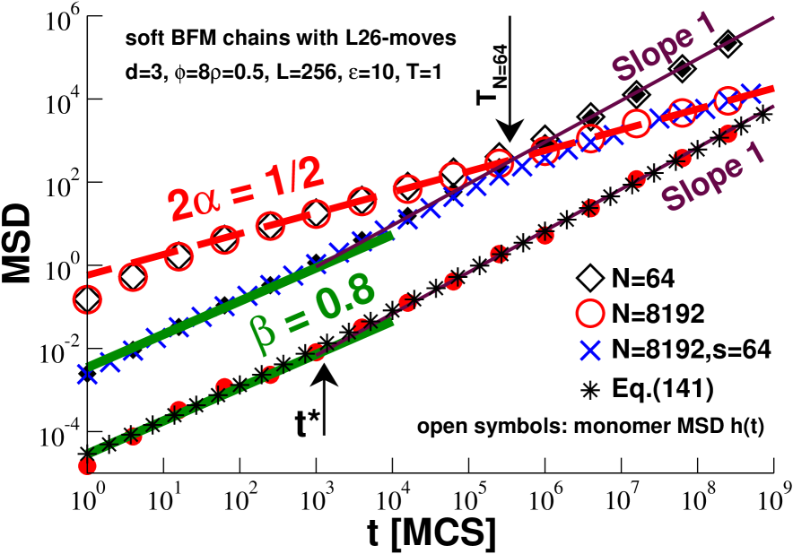
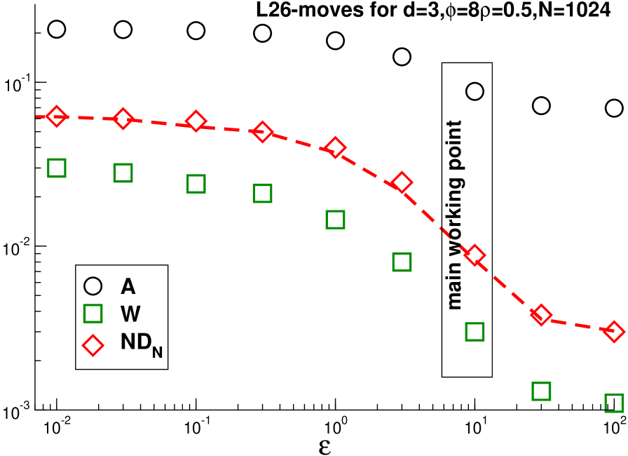
6.3.1 Mean-square displacements
Having shown that scale-free dynamical correlations exist for dense BFM beads as expected for overdamped colloids (Fig. 35), we turn now our attention to 3D melts of long and flexible homopolymers. As described in Sec. 3.4, we focus on systems with finite overlap penalty and volume fraction which we sample using local topology non-conserving L26-moves. As can be seen in Fig. 37 for chains of length and , these systems are essentially of Rouse-type. The monomer MSD is indicated by the open symbols.747474For the large sampled here it is inessential whether this average is performed over all monomers or only over a few monomers in the center of chains at as in Paul91a ; Paul91b ; KBMB01 . As expected from Rouse dynamics we obtain the -independent short-time asymptotics DoiEdwardsBook
| (136) |
indicated by the dashed line (). As can be seen for , the monomers diffuse again freely with a power-law slope (thin lines) for times larger than the Rouse time . We remind that it was neither computationally feasible nor our goal to sample for our larger chains () over the huge times needed to make this free diffusion regime accessible. Following Paul et al. Paul91b , the short-time power law, Eq. (136), can be used to determine the effective monomer mobility. We obtain for our main working point. Mobilities for other penalties are listed in Table 1. As may be seen from Fig. 38, decays with increasing excluded volume just as the acceptance rate (spheres) of the Monte Carlo attempts, but the decay is even more pronounced for , i.e. increasingly more accepted monomer moves do not contribute to the effective motion Paul91b .
The full symbols displayed in Fig. 37 refer to the MSD of the CM of chains of length . As one expects for Rouse chains, the amplitude of decreases inversely with and the diffusion appears to be Fickian () at least for times as indicated by the vertical arrow. Obviously, and merge for times beyond the Rouse time (). Fortunately, since becomes linear for , it is possible for all to measure the self-diffusion coefficient by plotting vs. time . For our main working point we obtain . Values for other are again given in Table 1 and are represented in Fig. 38 (diamonds). These values compare nicely with the Rouse model prediction DoiEdwardsBook
| (137) |
shown by the dashed line in Fig. 38. Similarly, it is possible (at least for our shorter chains) to measure the longest Rouse relaxation time by an analysis of the Rouse modes and to compare it with the Rouse model prediction DoiEdwardsBook . We obtain again a nice agreement between directly and indirectly computed relaxation times (not shown).
Up to now we have insisted on the fact that our systems are to leading order of Rouse type and we have characterized them accordingly. However, deviations from the Rouse picture are clearly revealed for short times, especially for .757575That the monomer MSD also deviates for very short times is due to the trivial lower cut-off associated to the discretization. In agreement with Eq. (13) the short-time CM motion may be characterized by a power-law exponent (bold lines). Since in our BFM version topological constraints are irrelevant, this shows that the deviations obtained for the classical BFM algorithm with topological constraints Paul91b cannot be attributed alone to precursor effects to reptational dynamics (which indeed exist as shown in Fig. 44).
Before we turn to the more precise numerical characterization of these deviations by means of the associated displacement correlation function, let us ask whether the observed colored forces acting for short times on the CM of the entire chain are also relevant on the scale of subchains of arc-length (). To answer this question we compute the MSD associated to the subchain CM as shown in Fig. 37 for subchains of length in the middle of total chains of length (crosses). Since for short times the subchain does not “know” that it is connected to the rest of the chain, one expects it to behave as a total chain of the same length (). This is indeed borne out by our data which are well described by
| (138) |
for all chain length and subchain length studied. The subchains reveal thus for sufficiently short times the same colored forces as the total chain as can be clearly seen from the example given in Fig. 37. For larger times the subchain becomes “aware” that it is connected to the rest of the chain and gets enslaved by the monomer MSD, i.e. as expected from the Rouse model we observe
| (139) |
and, obviously, for even larger times .
6.3.2 Locality and relevant exponent
Two comments are in order here. First, it should be noticed that Eq. (138) expresses the fact that the effective forces acting on the subchains of length in a chain of total length add up independently to the forces acting on the total chain. In this sense Eq. (138) states that the deviations from the Rouse picture must be local. We will explicitly verify this below (Fig. 41).767676The “locality” of the correlations described by Eq. (138) or Eq. (143) does not imply that the displacements of subchains around the reference subchain displaced at are -correlated. Second, if one chooses following Eq. (135) an arbitrary time window to characterize the displacement correlations, this corresponds to dynamical blobs containing adjacent monomers, which must move together due to the chain connectivity. Eq. (139) implies now that the dipole field777777We remind that, strictly speaking, it is not the dipole field associated to the density of the subchain center-of-masses, but to their chemical potential. The use of the imprecise notion “density dipole field” might be excused by the fact that both fields are supposed to decay similarly with time , chain length and subchain length . associated with the CM of these -subchains and created at by a tagged -subchain must decay according to a typical displacement with . It is this exponent which is mentioned in Eq. (134). Since this exponent is smaller than for colloids (), the subchain field must decay more slowly and one thus expects a much weaker decay of the associated VCF.
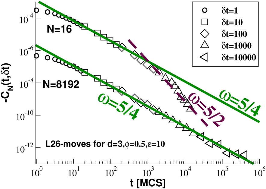
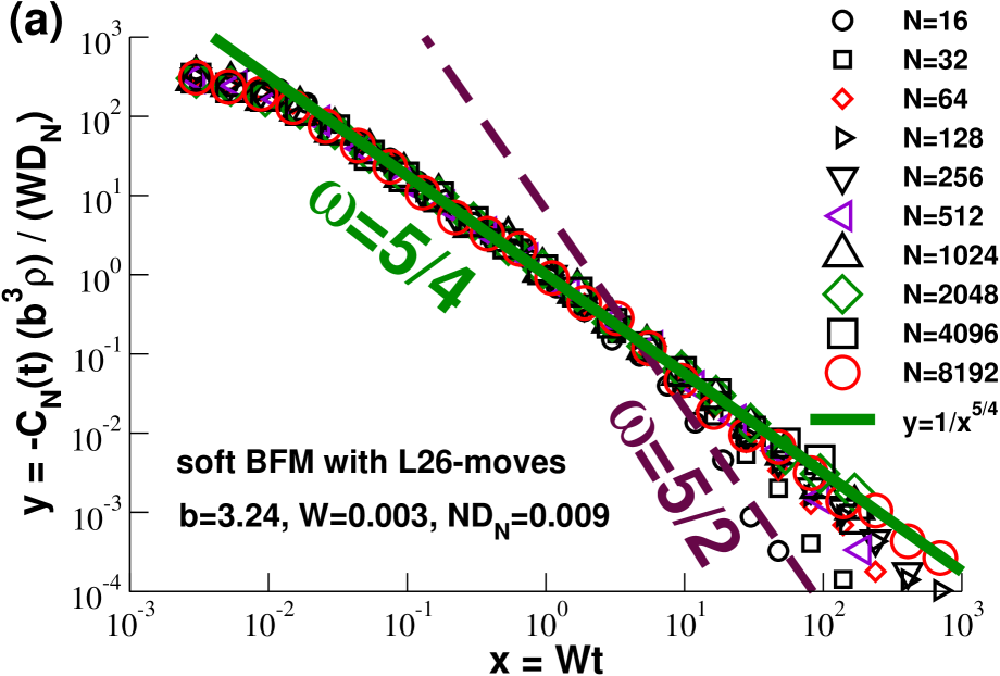
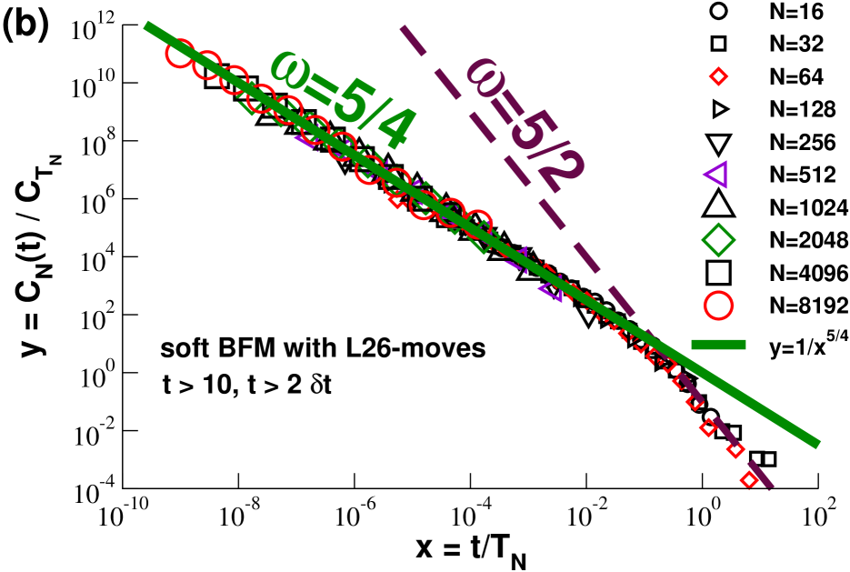
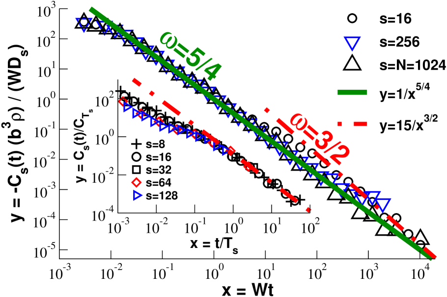
6.3.3 Center-of-mass velocity correlation function
Following the numerical strategy presented in Sec. 6.2, we characterize now more precisely the correlations seen for the chain MSD and the subchain MSD by computing directly their second derivative with respect to time , i.e. the associated correlation functions and .
The VCF for the displacement vector of the chain CM is shown in Fig. 39 for two chain lengths, (top) and (bottom). Averages are again performed over all configuration pairs in the set of configurations sampled for each . As in Sec. 6.2 we find that for . For clarity, only the data subset is indicated for each which is used to construct the final VCF (as shown below in Fig. 40). The bold lines represent the predicted short-time exponent which can be observed for over nearly five orders of magnitude. For we also indicate the exponent (dashed line) for where the polymers should behave as colloids according to Eq. (132). Note that the magnitude of the signal decreases strongly with , which together with the fact that fewer chains per box are available, makes the determination of increasingly more delicate.
The -dependence of the VCF is further analyzed in Fig. 40. The rescaled VCF is traced in panel (a) as function of the reduced time using the monomer mobility and the diffusion coefficient determined above (Table 1). This scaling makes the axes dimensionless and rescales the vertical axis by a factor . As shown by the successful data collapse for chain lengths ranging from up to on the slope indicated by the bold line, the VCF scales exactly as for . This confirms the already stated “locality” of the correlations, Eq. (138), i.e. the forces acting on subchains add up independently to the forces acting on the entire chain. We have still to motivate the precise scaling used for the axes. According to Eq. (133) the VCF scales as a function of the reduced time . Substituting the typical chain size and relaxation time this reduces for to
| (140) |
with being a dimensionless constant. The bold slope indicated in the plot corresponds to a value . Interestingly, since , it follows from Eq. (140) that
| (141) |
As may be seen in Fig. 37 (stars) for , Eq. (141) with provides an excellent fit of the measured . We also note that the second term in Eq. (141) dominates the short-time dynamics for . This is indicated by the vertical arrow in Fig. 37. Hence, for the stars correspond to a power-law slope with exponent . This is close to the phenomenological exponent from the literature. The central advantage of computing the VCF lies in the fact that it allows us thus to make manifest that (negative algebraic) deviations from the Rouse behavior exist for all times and not just for .
Returning to our discussion of Fig. 40(a) we emphasize that the VCF of shorter chains decay more rapidly for large times following roughly the exponent expected for effective colloids. We verify explicitly in Fig. 40(b) that the bending down of the data is consistent with the announced scaling in terms of a reduced time and a vertical axis using the amplitude stated in Eq. (133). The successful data collapse confirms that the only relevant time scale in this problem is the relaxation time for which the deviations for short () and long times () match. It is worthwhile to emphasize that the general scaling Eq. (133) together with the locality of the deviations, , immediately imply the exponent . This can be seen by counting the powers of the chain length ,
| (142) |
thus in agreement with Eq. (134) and the numerically observed time dependence. Assuming that Eq. (133) holds, the exponents for and thus contain the same information.
The VCF for subchains of arc-length is presented in Fig. 41. The subchain VCF is obtained as the total chain VCF , the only difference being that the CM of the subchain defines now the displacement vector . The data presented in the main panel is rescaled as in Fig. 40(a) with setting now the relevant diffusion constant used for the vertical axis. At short times the data for all collapses on the same power-law slope with exponent (bold line) as in Eq. (140). Confirming Eq. (12) and Eq. (138) we obtain the scaling
| (143) |
i.e. the colored forces acting on subchains add up independently to the colored forces acting on the total chain.
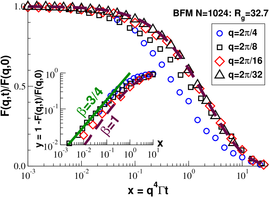
6.3.4 Dynamic coherent form factor
Neither the MSD nor the VCF of the (sub)chain CM can be measured directly in a real experiment. We discuss now how the exponent may be tested experimentally by means of the dynamical coherent form factor DoiEdwardsBook ; BenoitBook
| (144) | |||||
| (145) |
where stands for the Fourier transform of the density of a labeled chain. For the dynamical form factor reduces to the static form factor discussed in Sec. 5.7. In the Guinier regime probes the overall chain motion which allows to determine quite generally using the expansion DoiEdwardsBook
| (146) |
at least if sufficiently precise small angle data are available Smith00 ; PaulGlenn . Thus, for . Obviously, Eq. (146) also holds for our numerical data (not shown).
Larger wavevectors () are experimentally more readily accessible BenoitBook . Since in this regime the dynamical form factor probes the MSD of subchains of arc-length with replacing in Eq. (146) WMJ10 , it is of relevance to verify whether it is possible in practice to confirm the exponent using the numerically computed dynamical form factor. We remind that since in this wavevector regime becomes independent of , the Rouse model implies the scaling
| (147) |
being the scaling variable and
| (148) |
a rescaled monomer mobility DoiEdwardsBook . Using the directly measured mobility we have for the BFM data presented in Fig. 42. As can be seen from the main panel, a satisfactory data collapse is indeed obtained if sufficiently large subchains are probed (). This is consistent with the fact that our systems are to leading order of Rouse-type, especially if large times are probed. The scaling function indicated by the dashed line has been obtained by integrating numerically the Rouse model prediction DoiEdwardsBook
| (149) |
Considering that there is no adjustable parameter this fit is satisfactory. Expansion of Eq. (149) for small yields787878Note that the approximation given in DoiEdwardsBook is unfortunately wrong. Effective mobilities determined using this formula are therefore also incorrect WPB92 . A better approximation taking into account the fluctuations around the saddle point is given by .
| (150) |
Thus, according to the Rouse model one expects the rescaled dynamical form factor traced in the inset of Fig. 42 to increase (to leading order) as with (dashed line). Instead we find for larger wavevectors a power-law increase with exponent (bold line) in agreement with the scaling relation
| (151) |
for [Eq. (141)].797979That with decreasing wavevector the data approaches systematically the Rouse prediction is expected (i) since for the same value a smaller wavevector corresponds to a larger time and (ii) since for the colored noise becomes masked by the white forces, Eq. (141). In other words, an experimental observation of a power law slope of the reduced dynamical structure factor with would thus confirm scale-free CM displacement correlations with .
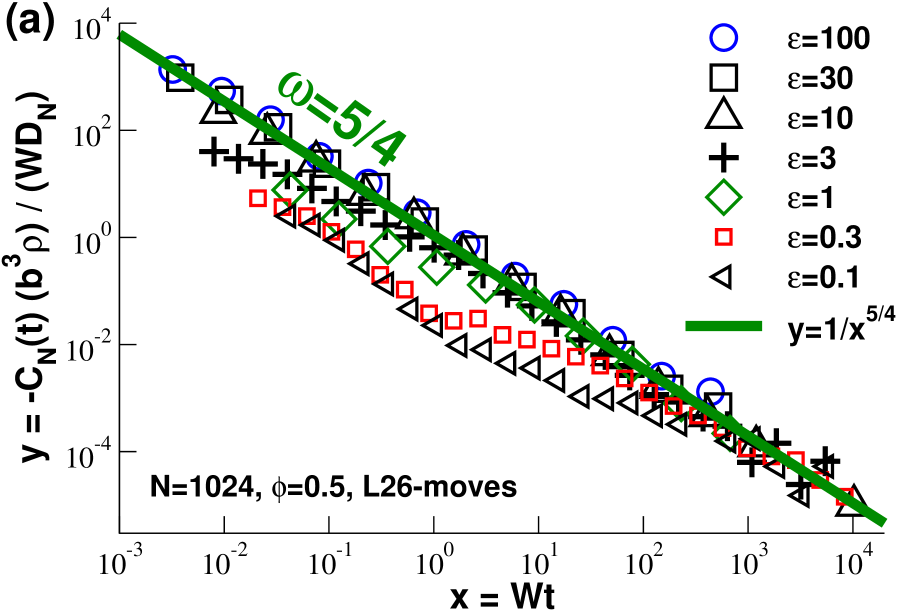
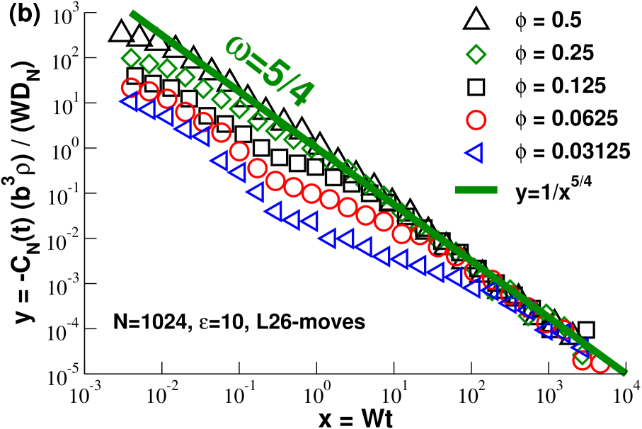
6.4 Compressibility effects
Up to now we have focused on one working point at overlap penalty and volume fraction , i.e. all data corresponds to the same static properties, especially to the same dimensionless compressibility . It is natural to ask how the observed scaling changes with the compressibility of the solution. Our key scaling relation Eq. (133) corresponding to an incompressible packing of blobs does in fact only depend implicitly on . This suggest that Eq. (140) for times should also remain valid if one uses for rescaling of the axes the effective bond length , the mobility and the diffusion constant measured independently for the given operational parameters and . This is in fact borne out for the asymptotic behavior of the rescaled VCFs displayed in Fig. 43(a) for different overlap penalties at and in Fig. 43(b) for different volume fraction at . (We only display chains with to avoid the colloidal regime for .) The values used for the rescaling of the axes are listed in Table 1 for the variation of the overlap penalty and in Table 2 for different volume fractions. The scaling collapse for long times presented in panel (b) demonstrates explicitly that if one scales out the additional variation of the monomer mobility . We remind that this density dependence stems originally from the factor in Eq. (133) due to the correlation hole forces setting the repulsion between chains and subchains which drive the dynamical correlations. That the data deviates for short time from Eq. (140) is to be expected qualitatively since the incompressibility constraint is only felt by the chains if the dynamics is probed on a scale corresponding to the static screening length. As we have seen in Sec. 5.4, a similar crossover is observed for static properties such as the angular correlation function WCK09 . At present we are still lacking a detailed description for the short time dynamical behavior and how to match it with the correlated motion of incompressible blobs at long times.

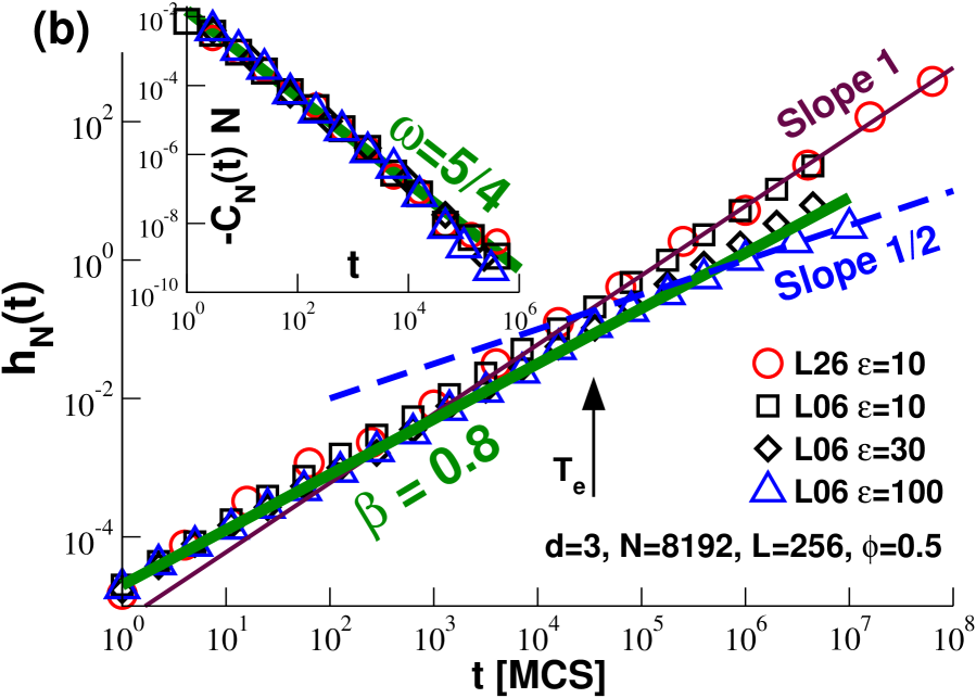
6.5 L06-moves and effects of topological constraints
Up to now we have deliberately tuned our model to avoid topological constraints. Obviously, these constraints are expected to matter for the dynamics of real 3D polymer melts DegennesBook ; DoiEdwardsBook . It is thus of interest to see how the presented picture changes if topology is again switched on using the topology conserving L06-moves of the classical BFM Paul91a ; Paul91b ; KBMB01 .
Obviously, for small penalties the dynamics remains of Rouse-type as can be seen from Fig. 44(a) for the same static conditions (,) as in Sec. 6.3. One determines readily a local mobility and a self-diffusion coefficient , i.e. the dynamics is slightly slower than for the larger L26-moves. If using these parameters is rescaled as shown in Fig. 40(a), all data sets collapse perfectly on the same slope as for L26-moves (bold line). This is consistent with the idea that the scaling Eq. (140) only depends implicitly on the specific MC moves used.
Preliminary data comparing L26-moves and L06-moves for chains of length and higher overlap penalties is presented in Fig. 44(b). With increasing the crossing of the chains gets more improbable for L06-moves and the topological constraints become more relevant. This can be seen for and even more for . The latter data set approaches the slope (dashed line) expected from reptation theory for times larger than the entanglement time DoiEdwardsBook . The vertical arrow indicates a value for obtained from an analysis of the monomer displacements KBMB01 . Apart from the much larger chain length used, the data for is consistent with the results obtained using the classical BFM () Paul91b ; KBMB01 . As in Fig. 37 the bold line represents the exponent Paul91b ; PaulGlenn . Superficially, it does a better job for systems with conserved topology due to the broad crossover to the entangled regime. However, that this empirical exponent is by no means deep as revealed by the VCF plotted in the inset. For short times all systems with and without topology conservation are well-described by the same exponent (bold line) in agreement with the proposed deviations from the Rouse model, Eq. (134). Note that the last points given for decay slightly more rapidly. Unfortunately, the length of the analyzed time series does currently not allow us to verify whether our data become consistent with the decay
| (152) |
expected for reptating chains with being the tube diameter DegennesBook . Much longer time series, just as for the L26-moves with we have focused on, are currently under production to clarify this issue. The numerical demonstration is challenging, since the difference between the exponents, , is rather small and several orders of magnitude in time are needed to discriminate the power laws. In any case it is thus due to the dynamical correlations first seen in the BFM simulations of Paul et al. Paul91b ; PaulGlenn that the crossover between Rouse and reptation regimes becomes broader and more difficult to describe than suggested by the standard Rouse-reptation theory DegennesBook ; DoiEdwardsBook which does not take into account the (static and dynamical) correlations imposed by the incompressibility constraint.
6.6 Perturbation calculation predictions
6.6.1 Colored collective forces
Focusing now on the short-time correlations () in -dimensional polymer melts without topological constraints, we present now a linear response calculation to describe the coupling between the degrees of freedom of a tagged test chain and the degrees of freedom of the collective bath characterized, respectively, by the dynamical form factor and the dynamical structure factor at equilibrium. The underlying physics is that the displacement of a test chain at creates a free energy perturbation of the bath which decays by collective diffusion but survives at intermediate times. The collective force associated with the perturbation of the molecular field pushes the test chain towards its original position at causing thus the anomalous diffusion of the CM motion demonstrated numerically above. We remind first that the forces acting on the CM of an a priori Rouse chain may be written DoiEdwardsBook
| (153) |
i.e. in addition to the random white force of the standard Rouse model we have to account for the force from the molecular field. The friction coefficient may be obtained using Eq. (148) from the effective monomer mobility . According to the relation Eq. (176) given in Appendix A, the VCF of the chain CM is given by
| (154) |
i.e. our task is to compute the correlation of the collective force due to the molecular field surrounding the reference chain. The negative sign corresponds to the fact that the collective forces push the reference chain back towards its original position, just as for the overdamped colloids.
6.6.2 Dynamical random phase approximation
As already discussed in Sec. 6.3.4, the degrees of freedom of the test chain are encoded by the dynamical form factor , Eq. (145). As seen from the main panel of Fig. 42, the scaling with is nicely obeyed for not too large wavevectors, although deviations from the Rouse prediction are visible for small . Since these deviations are small, it is justified in the spirit of a perturbation calculation to assume that Eq. (149) holds for all wavevectors and times .

The degrees of freedom of the bath are described by the dynamical collective structure factor
| (155) |
with being the Fourier transform of the collective monomer density. For Eq. (155) reduces to the static structure factor analyzed in Sec. 4.4. The dynamical structure factor cannot be devised using the Rouse theory alone, for encodes the collective behavior of the chains, a cooperativity destroyed by the assumptions underlying the Rouse approach. Fortunately, to deal with this question the “dynamical Random Phase Approximation” (dRPA) is a valuable tool which provides sensible predictions for ANS86 ; ANS97b ; papFarago . Similarly to the static RPA discussed in Sec. 4.4, the dRPA is based on a self-consistent closure of a mean-field theory: upon a perturbation by an external field, the response of a polymer is assumed to be the combination of a direct response to the field plus a response mediated by the environment of other chains, which are also subjected to the external field. This autocoherent reasoning leads to a prediction for , the Laplace transform of , given by papFarago
| (156) |
with being the effective monomer excluded volume and the Laplace transform of the dynamical form factor . For , i.e. by summing over all times , this equation yields of course the static RPA discussed in Sec. 4.4. Using this limit one may rewrite Eq. (156) which yields the dRPA formula
| (157) |
Focusing on incompressible systems (), large wavevectors () and short times , Eq. (157) can be further simplified. As shown in papFarago
| (158) |
where and stand, respectively, for the Laplace transform of the scaling functions and . Assuming for the Rouse model prediction, Eq. (149), this yields for the bold line presented in Fig. 45. Taking apart deviations for small , i.e. for small times, we obtain a nice scaling collapse for the BFM data presented in Fig. 45, especially considering that there is no free fit parameter available. We note finally that since for the wavevectors used , it follows from Eq. (158) that
| (159) |
for sufficiently low wavevectors at fixed compressibility or for sufficiently small compressibilities at fixed wavevector.
6.6.3 Lowest-order perturbation
A collective density fluctuation corresponds to a molecular field driving the monomers of the test chain with a force . The lowest order force correlation corresponds to the following mechanism: the test chain interacts with the collective field at time and again at time . Using the densities and of the test chain and the bath in Fourier space defined above, the collective force may be rewritten as
| (160) |
The correlation for becomes thus after lowest-order factorization
| (161) |
Using the dynamical form and structure factors, Eq. (145) and Eq. (155), this yields
| (162) |
Using Eq. (154) and Eq. (159) the VCF becomes
| (163) |
Since and decrease rapidly for , the integral is well-behaved. After substituting the friction coefficients and by , Eq. (148), this may be rewritten as
| (164) |
Hence, Eq. (164) confirms finally the scaling announced in Eq. (133) and Eq. (134). The coefficient is given by
| (165) |
which may be computed numerically papFarago . For 3D melts () we find . This is of the same order but slightly lower as the empirical coefficient estimated from Fig. 40. Where this small difference comes from is currently still an unresolved question. One possibility is that the single loop approximation presented here — especially assuming Eq. (149) and Eq. (158) for small — is not sufficient and higher order terms should be considered. Another (physically more appealing) option is that only about half of the free energy is stored in the longitudinal composition fluctuations and that the transverse stress due to the shearing of the bath at constant density generates an additional contribution to the correlations of same magnitude papFarago ; ANS11b .
6.7 Summary
Focusing on a variant of the BFM algorithm with topology non-conserving moves we investigated the effective dynamical forces acting on the chains and subchains imposed by the incompressibility constraint. Sampling chain lengths up to allowed us to carefully check the -dependence of deviations with respect to the Rouse model. Such deviations are visible from the short-time scaling of the CM MSD in agreement with the literature, however, a more precise characterization can be achieved by means of the CM VCF which allows to probe directly the correlated random forces, Eq. (154). How such a VCF can be computed within a MC scheme has been first illustrated for dense BFM beads (Fig. 36) confirming the negative algebraic decay expected for overdamped colloids, Eq. (132). The observed exponent with can be understood by the coupling of a tagged colloid to the gradient of the collective density field decaying in time. As shown in Fig. 40(b), the same exponents are relevant for polymer chains for large times () where the chains behave as effective colloids. More importantly, the short-time deviations for have been traced back to the negative analytic decay for with an exponent . That decays inversely with mass shows that the process is local, i.e. the displacement correlations of subchains of arc-length add up independently (Fig. 41). Assuming according to the postulated scaling relation Eq. (133) the chain relaxation time to be the only characteristic time scale, both asymptotic regimes can be brought to a successful data collapse. The -exponents for short times proposed in Eq. (134) are consistent with the crossover scaling, Eq. (133), and the locality of the correlations () which implies . This scaling can be understood by the generalization of the above-mentioned correlation experienced by overdamped colloids to the displacement field of subchains of length with being the (arbitrary) time window used to define the displacements. Since subchains repel each other due to the incompressibility constraint, a tagged subchain is pulled back to its original position by the subchain dipole field. Since for times the relevant dipole field decays much slower than for colloids (), the correlations are much more pronounced. That our scaling relations for do not depend explicitly on the compressibility of the solution, as stated by Eq. (133), has been checked by the systematic variation of excluded volume penalty and volume fraction WPC11 . As shown for melts with topological constraints the early-time behavior, , is preserved before entanglement effects set in which leads to a broad crossover between Rouse and reptation regimes. As shown in Sec. 6.6, our scaling approach is consistent with a standard linear response calculation. En passant we have verified the so-called “dynamical Random Phase Approximation” for the collective dynamical response of the bath surrounding the reference chain (Fig. 45) papFarago .
7 Conclusion
7.1 Summary
Until very recently it has been generally assumed that all long-range static and dynamical correlations are negligible in dense 3D solutions of flexible homopolymers beyond the excluded volume screening length which characterizes the decay of the density fluctuations FloryBook ; DegennesBook ; DoiEdwardsBook ; RubinsteinBook . For static properties this general screening assumption leads to Flory’s ideality hypothesis (Sec. 1.3) FloryBook ; DoiEdwardsBook stating that the chains must obey Gaussian chain statistics. For the equilibrium dynamics it implies Rouse model dynamics (Sec. 1.4) if in addition momentum conservation (“hydrodynamic screening”) and topological constraints DoiEdwardsBook may be neglected or are deliberately switched off as one can readily do in a computer experiment using local MC hopping moves (Sec. 3.3.1).
That some deviations from Flory’s ideality hypothesis must exist has been suggested in earlier work by de Gennes DegennesBook ; Brochard79 , Obukhov Obukhov81 , Duplantier Duplantier89 , Schäfer et al. SchaferBook ; MM00 or Semenov and Johner ANS03 . For instance, it has been known for a long time DegennesBook that due to the incompressibility constraint an entropic penalty set by the correlation hole self-density has to be paid for bringing two chains of length close to each other (Fig. 3). In the large- limit this effect must become negligible in , however. That the dynamics of polymer melts without relevant topological interactions may deviate from the Rouse model has been pointed out in various theoretical, computational and experimental studies by Schweizer Schweizer89 , Guenza et al. Guenza02 or Paul et al. Paul91b ; Paul98 as summarized in Ref. PaulGlenn . However, since topological and hydrodynamical effects have not been systematically separated from the incompressibility constraint Guenza02 — with the notable exception of the BFM simulations of Shaffer Shaffer94 ; Shaffer95 — it has been difficult to pin-point the precise physical origin of the key finding observed for the MSD of the chain CM, Eq. (13).
Summarizing recent theoretical and computational results we have argued in the present contribution that due to the incompressibility constraint both static WMBJOMMS04 ; WBCHCKM07 ; WBJSOMB07 ; BJSOBW07 ; WBM07 ; MWK08 ; WCK09 ; WJO10 ; WJC10 ; ANS10a and dynamical WPC11 ; papFarago correlations of the composition fluctuations, i.e. of the density and displacement fields of marked chains and subchains, must arise for distances and for corresponding arc-lengths . Since the applied constraint is scale-free, the resulting correlations are also scale-free — taken apart the usual upper and lower cutoffs set by the chain and the monomer size — and do not depend explicitly on the dimensionless compressibility of the solution (Sec. 2.3). The central point stressed by us WBCHCKM07 is that not only chains but also subchains of arbitrary length must repel each other due to the incompressibility constraint and this with a penalty being for much larger than the penalty between the chains (Fig. 4). Since subchains repel each other and this with a strength decreasing with in , the chains become weakly swollen as discussed in Sec. 5. Our study shows that a polymer in dense solutions should not be viewed as one soft sphere (or ellipsoid) EM01 ; Likos01 ; Guenza02 , but as a hierarchy of nested segmental correlation holes of all sizes aligned and correlated along the chain backbone [Fig. 3(b)].808080Similar deviations from Flory’s ideality hypothesis have been reported recently for polymer gels and networks Sommer05 ; Everaers05 . The effective interaction between subchains has also dynamical consequences since a subchain displaced at causing thus a perturbation of the subchain density field (Fig. 35) will be slightly pushed back by the bath to its original position (Sec. 6).
In this review we have focused on numerical results obtained by means of a BFM variant with finite monomer interactions without topological constraints (Fig. 6). Since this “soft BFM” is fully ergodic (in contrast to the classical BFM) and very efficient due to its implementation as a Potts spin model WCK09 , it may be an interesting alternative to various popular coarse-grained simulation approaches with self-consistently calculated effective pair interactions EM01 ; Likos01 ; Guenza02 ; MMuller05 ; MMuller06 . Our study has not been limited to monodisperse polymers but we have also investigated (essentially) Flory-distributed EP WBCHCKM07 ; BJSOBW07 ; WJO10 ; WJC10 . Since in these systems chains break and recombine constantly (Fig. 9) equilibration and sampling become much faster than for their monodisperse counterparts. This is computationally of interest since the numerical demonstration of the various theoretical predictions requires the sampling of large chain lengths to avoid additional chain end effects.
The deviations from the screening assumption are indeed scale-free as made manifest by the numerical observation of the analytic decay of various correlation functions. As announced by Eq. (11), it has been shown in Sec. 5 that the bond-bond correlation function decays as for and . That these correlations are long-ranged is made explicit by the power-law decay of the bond-bond correlation function as a function of the monomer distance (Sec. 5.4.2). As a second key result of this study, the displacement correlation function is shown to reveal for short times a negative algebraic decay according to as predicted by scaling arguments and perturbation theory (Sec. 6). As stated by Eq. (12), this analytic decay holds more generally for the displacement correlation function of subchains of length and times , Fig. 41, which shows that the correlations of different subchains add up independently to the correlations of the total chain (“locality”).
Note that earlier computational studies have focused on (second and higher) moments of the generalized displacement field under consideration such as the mean-squared size of subchains of arc-length Auhl03 or the CM MSD Paul91b and have thus only probed indirectly the respective colored forces, Eq. (176), corresponding to the deviations from the general screening assumption.818181In line with Appendix A we view here the bond vectors of a chain conformation as displacement vectors with the monomer index playing the role of time. Computing numerically correlation functions such as or , rather than twice their integral, allows to probe directly the colored forces, Eq. (176), without having to subtract first the white noise and the local physics which contribute both to and . As a consequence, this allows to demonstrate that the deviations from the screening assumption are not due to (non-universal) physics at the lower cutoff but, in fact, are present for all arc-length (Fig. 25) and all times (Fig. 40).
7.2 Related questions and outlook
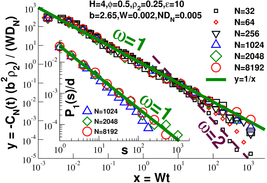
7.2.1 Confined polymer melts
In the presented numerical work we have focused on 3D polymer bulks (). It has been shown that even the deviations with respect to the general screening assumption are well-described by means of one-loop perturbation calculations (Sec. 2, Sec. 6.6) and this for arbitrarily long chains and subchains. As already noted in Sec. 1.1, the success of the mean-field approach is expected due to the scaling of the (sub)chain self-density , i.e. the number of subchains a reference subchain interacts with increases as in . Due to the increasing experimental interest on mechanical and rheological properties of nanoscale systems in general NanoscienceBook and on polymer melts confined to surfaces, thin slits () or capillaries () in particular Russel96 ; RLJones1999 ; mai99 ; Granick03 ; Russel04 ; McKenna2005 ; Deutsch05 ; Rubinstein07 ; Obukhov07 one is naturally led to question theoretically such mean-field calculations for systems of reduced (effective) dimension Brochard79 ; Duplantier89 ; ANS03 ; LFM11 ; EisenrieglerBook ; Saleur03 ; Saleur07 . Especially, the perturbations to chain dynamics due to geometric constraints remain a challenge of significant technological relevance with opportunities ranging from tribology to biology Russel96 ; RLJones1999 ; Granick03 ; McKenna2005 .
Note that for ideal chain systems with the self-density ultimately exceeds the density at a characteristic chain length which depends on the specific problem considered. For (sub)chains larger than this length one expects the chains to adopt compact and segregated conformations, i.e. Flory’s exponent is given by the spatial dimension, MandelbrotBook . Since these compact structures arise ultimately due to the scale-free incompressibility constraint, their surfaces are expected not to be ruled by a finite surface tension (which would imply a length scale) ANS03 ; MSZ11 but to be also scale-free and described by a fractal surface exponent MandelbrotBook . In most cases of interest the surface exponent becomes MSZ11 , i.e. it is set by the well-known contact exponent describing the scaling of the distribution for short distances between two monomers and on a chain. (Obviously, for Gaussian chains, Eq. (2).) According to the generalized Porod law the intramolecular structure factor of such compact objects scales as
| (166) |
in the intermediate range of the wavevector BenoitBook ; bray88 ; MSZ11 . If , i.e. , the standard Kratky representation reveals thus a much more pronounced non-monotonous behavior as for the 3D melts discussed in Sec. 5.7.828282Incidentally, melts of non-concatenated rings in have been argued to become “marginally compact” with and , i.e. the form factor is predicted to scale as MSZ11 ; KK11a in the large- limit. That the rings should adopt compact configurations is expected due to the mutual repulsion caused by the topological constraints MWC96 ; MWC00 ; MWB00 ; Gagliardi05 ; Cates86 ; Obukhov94 ; winkler06 ; Vettorel09 ; suzuki09 ; KK11a ; winkler11 ; MSZ11 . Since there is no obvious reason for a finite surface tension, the surface must become fractal which may be determined both in experiment as in a computer simulation by the generalized Porod law of the form factor. A marginally compact structure allows to keep all monomers evenly exposed to the topological constraints imposed by other rings, i.e. all subsegments of the rings are thus ruled in a self-similar manner by the same statistics. Such behavior is known for various biological systems, such as the lungs of mammals, attempting to maximize the surface at constant overall embedding volume WBE99 .
Strictly 1D and 2D self-avoiding polymer melts () are known to become compact and segregated with and are thus not Gaussian beyond the monomer scale. While the 1D case is trivial, it should be noted that for strictly 2D melts compactness means DegennesBook . This does of course not imply ideal chain behavior since other critical exponents characterizing the chain conformations differ from those of non-interacting Gaussian chains as shown in the pioneering work by Duplanier Duplantier89 . For instance, since Duplantier89 this implies that the compact 2D chains have a fractal perimeter of dimension ANS03 . This theoretical prediction has been verified numerically MKA09 ; MWK10 ; MSZ11 from the scaling of the chain perimeter (determined by “box counting” MandelbrotBook ) and of the form factor shown to be consistent with Eq. (166).
Self-avoiding melts in strictly one and two dimensions correspond to rather specific universality classes ANS03 ; Saleur03 ; Saleur07 ; LFM11 . Since systems of strictly one monomer layer thickness at high volume fractions remain experimentally a challenge mai99 ; Deutsch05 , it is of interest to relax the non-crossing constraint by either allowing some finite monomer overlap penalty (Sec. 3.4) or by considering chains confined to capillaries or slits between parallel walls of finite distance as in Fig. 6(c). Note that for melts confined to a 1D capillary of finite width as already shown by Brochard and de Gennes in 1979 Brochard79 and is known to increase even exponentially with for essentially 2D ultrathin films ANS03 . Since becomes thus rapidly large, perturbation results, such as the scaling of the bond-bond correlation function stated in Eq. (11), must become relevant for finite (sub)chain lengths. A lower limit of validity of the -dimensional perturbation calculation is set for systems with finite overlap penalty by and (sub)chains confined to capillaries or slits of finite width should be larger than , otherwise the chains do not “feel” the wall constraint and behave as in the 3D bulk.
Let us focus now on effectively 2D films of width Cavallo03 ; Cavallo05 ; CMWJB05 ; thinfilmdyn as shown in Fig. 46. Note that all properties considered here are the 2D projection of the 3D observables. The relevant density is, e.g., the projected number density and the indicated bond length is the projection of the effective bond length of the 3D melt. Since the width used here is much smaller than the typical subchain size considered, i.e. , these systems can be regarded as effectively dimensional for all and . (We write to stress that monomer overlap and chain crossings are allowed.) Since also one expects the perturbation result for the bond-bond correlation function with to yield a reasonable fit to the measured data for all . This is indeed borne out nicely for the data presented in the inset. According to Eq. (4) this implies that and must increase logarithmically with, respectively, and . This can be checked directly as seen in Ref. CMWJB05 . The same paper also investigates the form factor for different . It is shown that becomes systematically more non-monotonous with decreasing width , i.e. the more increases.
We turn now to the dynamics of BFM melts confined to thin slits of width sampled using local topology non-conserving L26-moves as in Sec. 6.3 thinfilmdyn . It can be demonstrated that to leading order the dynamics remains consistent with the Rouse model, especially Eq. (5).838383Since in thin films the ratio diverges logarithmically with ANS03 ; CMWJB05 ; papEPslit and since still holds, there are some (rather weak) logarithmic corrections to Eq. (5) as discussed in thinfilmdyn . As before, we obtain from the monomer MSD a local mobility, . That the self-diffusion coefficient scales as can be seen by tracing in log-linear coordinates. (Note that and are consistent with Eq. (137).) Systematic deviations are again revealed by the short-time behavior of the MSDs and of chains and subchains (not shown). These deviations are, however, much more pronounced than in 3D and are visible over time scales up to the total chain relation time . A more precise characterization of the colored forces acting on the chains is again achieved by means of the VCF which is represented in the main panel of Fig. 46. The representation chosen is similar to Fig. 40(a) for the bulk case; the factor being replaced by . The faster decay observed for the shorter chains at is described by the exponent (dashed line) expected for 2D overdamped colloids, Eq. (132). As may be seen from the collapse for short times (), the VCF scales again as , i.e. the colored forces are again local.848484Note that a different scaling, , has been reported in a study of strictly 2D polymer melts sampled by MD simulation using a standard Langevin thermostat WMJ10 . The correlations of the CM motion are argued to become non-local in this special limit due to the “constant surface constraint” of the compact and segregated subchains. In agreement with Eq. (134) or Eq. (142) the VCF is observed to decay algebraically with an exponent (bold line). Since it follows that is not constant but must increase logarithmically for all times . In analogy to Eq. (141) for the bulk case this thus explains the observed deviations from the Rouse model.
7.2.2 Interchain correlations and anti-Casimir forces
The presented work has focused on intrachain properties such as the bond-bond correlation function . The main reason for this is that the power-law exponents associated to the intrachain static and dynamical deviations due to the incompressibility constraint are not too large being thus numerically still accessible with reasonable computational effort. In fact, similar correlations have been predicted theoretically also for interchain properties ANS05a ; ANS05b which for macroscopic thermodynamic and mechanical properties may even be more relevant. Note that for these interchain correlations it is not only the incompressibility constraint which matters but in addition the constraint that closed loops are disallowed and must be eliminated from an extended grand-canonical ensemble containing both linear chains and rings, as shown by Obukhov and Semenov ANS05a ; ANS05b . The “throwing-away” of configurations is argued to generate additional entropic forces repelling, e.g., two large colloids immersed in a linear-chain polymer melt. Unfortunately, these “anti-Casimir forces” correspond to such strong exponents as a function of distance or wavevector (similar to the standard van der Waals forces Israela ) that, at present, it has turned out to be elusive to verify them numerically although a brave attempt has been made by means of off-lattice MC simulations Milchev02 . Following this recent work, we sketch in Fig. 47 two possibilities which might allow to probe correlations due to the no-loop constraint by means of EP melts confined to thin slits. The use of EP instead of monodisperse chains should speed up the sampling of independent configurations while confining the monomers reduces the exponents of the various analytic scaling relations predicted. For instance, the second Legendre polynomial , measuring the orientation of the bonds at a distance from a small region where an external field weakly aligns the bond vectors, should decay as with for as illustrated in panel (a) of Fig. 47. If successful these simulations may stimulate real micro-mechanical experiments using optical tweezers aligning bond vectors and repelling thus nearby colloids.
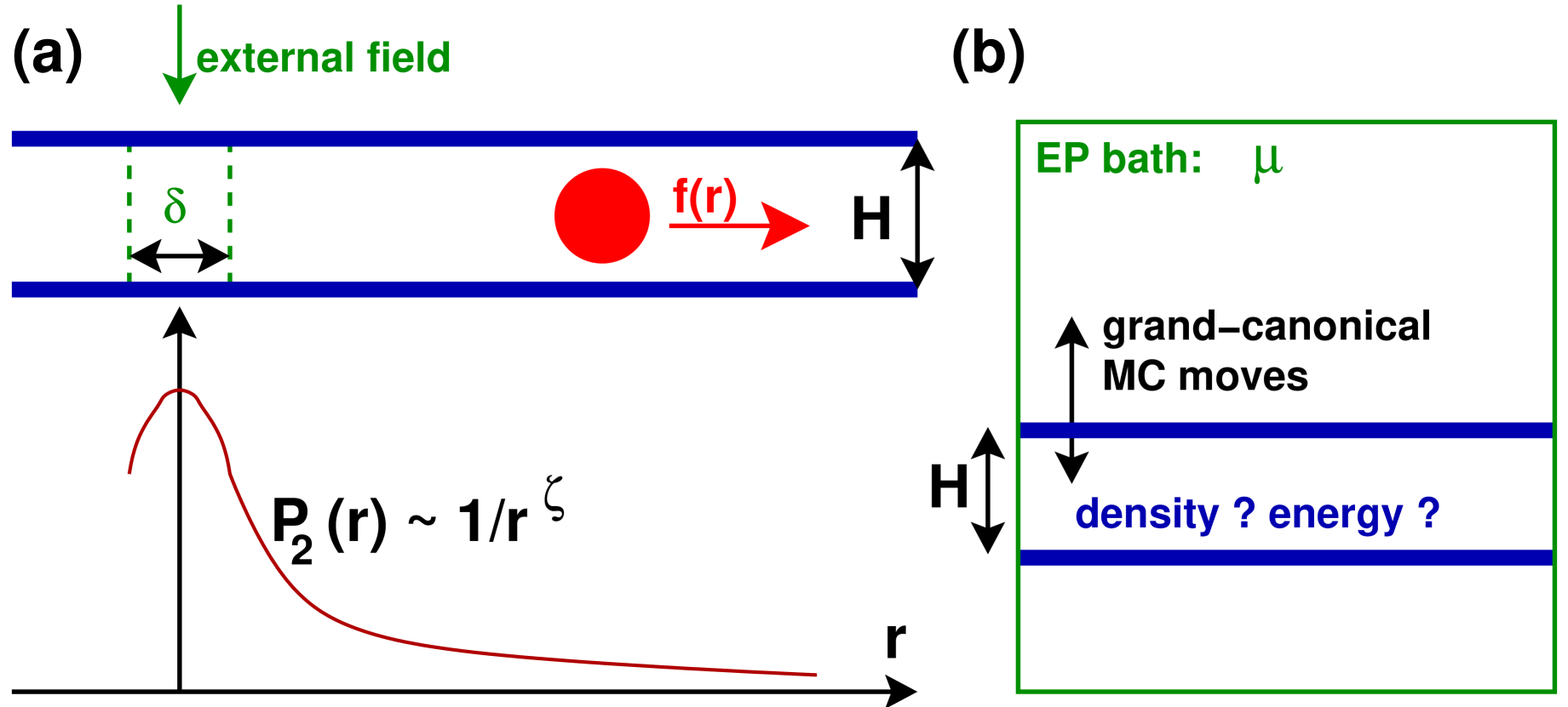
7.2.3 Dynamical properties beyond MC stochastics
We have checked by means of MD simulations of a bead-spring model papFarago ; ANS11a that for holds as long as a large friction constant is used for the Langevin thermostat applied FrenkelSmitBook . Concerning the power-law amplitude it should be noted, however, that the coefficient determined from the data using Eq. (140) is much larger for these MD simulations () compared to our BFM result (). As we have pointed out in Sec. 6.6, small differences of order one to the predicted value are expected due to the approximations made in the one-loop perturbation theory, especially since the forces associated to the shear stress may not be properly accounted for papFarago . However, the much larger ratio found for our MD simulations points to additional physics related to the screening of the monomer momentum in these strongly interacting viscoelastic systems ANS11a ; ANS11b .858585The beads bounce into each other on time scales much shorter than . Kicks due to conservative or random forces can thus propagate through the system before the thermostat has time to do its job. Since our BFM and MD simulations correspond to different model systems, it is currently not possible to clarify this issue. In the future we plan to address this problem using a generic (off-lattice) bead-spring Hamiltonian with soft beads and large springs such as, e.g., the model used by Spenley Spenley00 since we require a model which is (i) essentially incompressible (), (ii) without having too much useless local structure (as for the Lennard-Jones beads used in papFarago ; ANS11a ; ANS11b ), (iii) does not conserve topology and (iv) can be used for different dynamical methods such that we can compare the melt dynamics under the same static conditions. For such a model one should then compare the dynamics obtained by means of
-
MD simulation with a strong Langevin thermostat FrenkelSmitBook ;
-
local MC moves of the monomers LandauBinderBook ;
-
BD simulation in the sense of a “position Langevin equation” where the momentum variables are dropped from the equations of motion AllenTildesleyBook ; Ermak75 .
The BD method has the advantage that one needs not to inject strong random forces as for MD to get rid of the momentum to get closer to the overdamped motion assumption implicit to theory papFarago . We expect to obtain for the MC and BD simulations similar ratios as for our BFM study.
Interestingly, much stronger dynamical correlations are revealed ANS11a in MD simulations using a weak Langevin thermostat () or a momentum conserving “Dissipative Particle Dynamics” (DPD) thermostat Warren97 ; FrenkelSmitBook . As expected from the hydrodynamic screening assumption DoiEdwardsBook , the chains are described to leading order by the Rouse model, i.e. Eqs. (136), (137) or (149) hold. However, it is shown that some long-range correlations arise due to an intricate coupling of hydrodynamics (momentum conservation) and the (transverse) viscoelastic response of the bath following the displacement of a reference chain.868686Note the analogy to the static excluded volume screening discussed in Sec. 2. Although the chains are essentially described in by Gaussian chain statistics, not all long-range correlations vanish. As a consequence, even the VCF of subchains for depends now explicitly on the total chain length , i.e. the correlations are non-local with as suggested by the Zimm model. Since the scaling is still described by Eq. (133) this implies an exponent for short times. Hence,
| (167) |
which is the central formula real experimental data should be compared with. Although the VCF decays now more rapidly in time, it is stronger than the VCF for perfectly overdamped melts, since the -dependence in Eq. (167) is weaker. Note that at both mechanisms become of the same magnitude: . Using the same bead-spring model mentioned above it would now be of high interest to sample the dynamical response using
-
a DPD thermostat following the work by Spenley Spenley00 .
Obviously, these issues are clearly outside the realm of standard MC based stochastics which shows their limitations.
Acknowledgements.
We thank A.N. Semenov (Strasbourg), I. Erukhimovich (Moscow), M. Müller (Göttingen) and T. Kreer (Dresden) for helpful discussions. A.C. acknowledges the MIUR (Italian Ministry of Research) for financial support within the program “Incentivazione alla mobilità di studiosi stranieri e italiani residenti all’estero”, H.X. the CNRS for supporting her sabbathical stay in Strasbourg, J.E.Z. a grant by the ANR Blanc (FqSimPIB), P.P. a grant by the IRTG “Soft Matter Science” and N.S. financial support by the Région d’Alsace.Appendix A Displacement correlations
Let denote a (real valued) stochastic variable in some vector space with being a discrete or continuous index characterizing this variable. Examples are the position of the monomers of a given chain as a function of the monomer index (Fig. 1)878787This monomer index may be either a discrete (as in our study) or a continuous variable as, e.g., in Refs. MMuller05 ; MMuller06 . or the center-of-mass (CM) position of a chain of length as a function of a time measured by the discrete number of Monte Carlo Steps (MCS). We assume translational invariance of ensemble averaged properties with respect to , i.e. properties such as the “mean-square displacement” (MSD)
| (168) |
only depend on the difference and not on the absolute indices or . Taking advantage of the translational invariance, the ensemble average is often sampled over all available pairs of indices for a given . Examples for MSDs obtained as “gliding averages” are the typical segment size presented in Sec. 5.3.2 or the MSD of BFM beads () discussed in Sec. 6.2. In this review we consider essentially Fickian stochastic processes where the associated generalized MSDs are to leading order proportional to time , Eq. (3) or Eq. (6). Since the deviations with respect to the Fickian behavior are small, it is important to sample directly correlation functions corresponding to higher derivatives of with respect to time.
Since we have to deal with indices which may be either discrete or continuous, let us introduce the (forward) difference operator abramowitz defined by with being a function of our vector space and an arbitrary (typically) small shift of . Let us define the “velocity vector”
| (169) |
associated to and the “velocity correlation function” (VCF)
| (170) |
which measures the correlations of two velocities and . automatically vanishes if both vectors are uncorrelated. Note that is a four-point correlation function with respect to depending in general on the shift of the index. If both displacements become trivially correlated and we have . To see how and are related for let us apply twice the difference operator to Eq. (168). This yields
| (171) |
where we have used that the difference operator and the averaging procedure commute. Since the MSD can be assumed to be mathematically well behaved and using the translational invariance it follows on the other hand side that
| (172) |
Altogether this demonstrates that
| (173) |
in agreement with Eq. (4) for the bond-bond correlation function and with Eq. (7) for the chain velocity correlation function. Note that since does not depend on , does not depend on either in the limit .
The stochastic variables of interest in this review are described by a position Langevin equation of form vanKampenBook
| (174) |
with being the “friction constant” and the total “force” acting on which may be decomposed in a random white force contribution and a colored force stemming from the remaining (non-white) interactions of the degree of freedom under consideration with the bath and its constraints. Perfectly Fickian behavior would be obtained if only the white force contribution were present ().888888While and are both of zero mean, one may add in addition an external force which allows to determine the friction constant from the drift velocity: . For being the position of a monomer or the CM of a chain as a function of time , Eq. (174) corresponds to an overdamped motion as discussed in Sec. 6.2 for MC beads or in Sec. 6.3 for Rouse-like chains in the melt, Eq. (153). From Eq. (174) it follows for the displacement correlation function that
| (175) |
The total force correlation function at decomposes now into four contributions:
-
(a)
since is a white force,
-
(b)
since future white forces cannot be anticipated,
-
(c)
and
-
(d)
due to the odd -symmetry of the velocity ANS98b .898989Since this implies for the total force which in turn yields . The identity (d) is then obtained by substituting (due to (b)) and
Summing up over all contributions and using Eq. (175) it follows
| (176) |
i.e. the displacement correlation function probes directly the correlations of the colored force . This general result is used in Sec. 6.6 for the motion of the chain CM with time but does also apply for the monomer position as a function of the monomer index where the bond-bond correlation function measures the colored forces acting on the chain. It should be stressed, however, that in this case the forces noted in Eq. (174) do not correspond directly to the standard forces acting on the monomers in real time.
Appendix B Static properties
B.1 Moments and generating function
Higher moments of the segmental size distribution can be systematically obtained from its Fourier transform which is in this context sometimes called the “generating function” vanKampenBook . For ideal Gaussian chains the generating function is given by where we have used to simplify the notation. Moments of the size distribution are given by proper derivatives of taken at . For example,
| (177) |
with being the Laplace operator with respect to the wavevector . A moment of order is, hence, linked to only one coefficient in the systematic expansion, , of around . For our example this implies
| (178) |
in general and more specifically for a Gaussian distribution . The non-Gaussian parameters read, hence,
| (179) |
which implies (by construction) for a Gaussian distribution. As various moments of the same global order are linked to the same they differ by a multiplicative constant independent of the details of the (isotropic) distribution . For example, , , , with and denoting the spatial components of the segment vector . Using Eq. (179) for it follows that
| (180) |
i.e. the properties and discussed in Figs. 29 and 30 must be identical in general provided that is isotropic and can be expanded in .
B.2 Deviations of the segmental size distribution

We turn now to specific properties of computed for formally infinite polymer chains in the melt. In practice, these results are also relevant for small segments in large chains, , and, especially, for segments located far from the chain ends. These chains are nearly Gaussian and the generating function can be written as where according to Eq. (56) we have a small perturbation due to the effective interaction potential given by Eq. (66). In this paragraph we use for the bond length of the Gaussian reference chain of the perturbation calculation and for the measured effective bond length, Eq. (17). To compute the different integrals it is more convenient to work in Fourier-Laplace space () with being the Laplace variable conjugate to :
As illustrated in Fig. 48, there are three contributions to this perturbation: one due to interactions between two monomers inside the segment (left panel), one due to interactions between an internal monomer and an external one (middle panel) and one due to interactions between two external monomers located on opposite sides (right panel). In analogy to the derivation of the form factor described in Ref. BJSOBW07 this yields:
| (181) | |||||
where we have set . The graph given in the left panel of Fig. 48 corresponds to the first two lines, the middle panel to the third line and the right panel to the last one. Seeking for the moments we expand around . Having in mind chain strands counting many monomers (), we need only to retain the most singular terms for . Defining the two dimensionless constants and this expansion can be written as
where we have used Euler’s Gamma function abramowitz . The first leading term at each order in — being proportional to the coefficient — ensures the renormalization of the effective bond length . The next term scaling with the coefficient corresponds to the leading finite strand size correction. Performing the inverse Laplace transformation and adding the Gaussian reference distribution this yields the -coefficients for the expansion of around :
| (183) |
More generally, one finds
| (184) |
From this result and using Eq. (178) one immediately verifies that
| (185) |
where we have defined
| (186) |
for the effective bond length with . We remind that refers here to the bond length of the Gaussian reference chain while is the effective bond length for asymptotically long chains. Since our key interest is not as for Edwards to predict DoiEdwardsBook ; Edwards82 but to describe the deviations for finite from the Gaussian limit for which sets the relevant reference length scale. Setting thus this leads to Eq. (76) with being a fit parameter. Using Eq. (179) one justifies similarly Eq. (78) for the Gaussianity parameter .
The moments Eq. (185) completely determine the segmental distribution which is indicated in Eq. (73). While at least in principle this may be done directly by inverse Fourier-Laplace transformation of the correction to the generating function it is helpful to simplify further Eq. (181). We observe first that does diverge for strictly incompressible systems () and one must keep finite in the effective potential whenever necessary to ensure convergence (actually everywhere but in the diagram corresponding to the interaction between two external monomers). Since we are not interested in the wave vectors larger than we expand for which leads to the much simpler expression
| (187) | |||||
with . The first term diverges as for diverging . It renormalizes the effective bond length in the zero order term which is indicated in the first line of Eq. (73). The next two terms scale both as . Subsequent terms must all vanish for diverging and can be discarded. It is then easy to perform an inverse Fourier-Laplace transformation of the two relevant -terms. This yields
| (188) |
with . This is consistent with the expression given in Eq. (73).
B.3 Intramolecular form factor
The deviation of the intramolecular form factor from the Gaussian reference can be readily obtained from the deviation of the subchain size distribution in Fourier-Laplace space. Since we have for asymptotically long chains
| (189) |
where we focus on the intermediate scale-free wavevector regime which does not depend on the chain length distribution . Using Eq. (187) derived in Appendix B.2 one obtains
| (190) |
where only the third term of Eq. (187) contributes.909090The first term in Eq. (187) must be discarded as before since it only renormalizes the effective bond length and would also contribute to the reference form factor . Note that stands now for both the measured effective bond length and the bond length of the Gaussian reference chain. It follows from Eq. (190) that within first-order perturbation theory
| (191) |
which is equivalent to the prediction Eq. (14) made in the Introduction. Note that this perturbation result is consistent with the renormalization group calculations of semidilute solutions by Schäfer SchaferBook ; MM00 . This is of course expected since semidilute solutions may be considered as incompressible melts of (semidilute) blobs DegennesBook .
B.4 Angular correlations
We present here the direct perturbation calculation of the bond-bond correlation function of Flory-distributed linear chains in reciprocal space following the discussion in Sec. 2.4.6. As sketched in panel (b) of Fig. 5, one only needs to compute the interaction diagram between the monomers of the two dangling tails if the two bonds and are placed outside the subchain of length connecting the head of the first bond with the tail of the second bond . To simplify the notations we set immediately and and do not distinguish between the bond of the computer model connecting the monomers and the effective Gaussian bond length , i.e. we set . Restating Eq. (80) the relevant interaction diagram reads919191The diagram in reciprocal space is very similar to the diagram indicated in Fig. 49 for the calculation of the bond-bond correlation function as a function of distance . Since for we want to sample at constant between the bond pairs irrespective of the distance between the bonds no momentum needs to be injected in the diagram and the momentum flowing along the diagram is constant everywhere.
| (192) |
The negative sign in front of the integral is due to the negative sign of the general perturbation calculation formula Eq. (57). The first factor in the integral over the wavevector stands for the Fourier transformed Gaussian propagator between the two bonds indicated in Fig. 5(b). Using Eq. (82) the scalar product of the bond vectors in real space is represented by the scalar product of the wavevectors flowing through the bonds. Note that the momentum flows in the same direction as the two bonds and the operator thus reads . We assume that chains are Flory-distributed and that the effective interaction between two monomers in the two dangling ends is described by Eq. (65). The combinatorics between the interacting monomers — corresponding to the second line in Eq. (79) — leads using Eq. (29) to an additional weight factor
| (193) |
for the two Flory-distributed dangling tails. The task is thus to compute
| (194) |
where we have used that , Eq. (44). Rewriting the last factor in Eq. (194) as
| (195) |
and defining the integral
| (196) |
one may rewrite the interaction integral as
| (197) |
We remind that the integral takes the asymptotics
| (198) |
Considering thus the limit of infinite Flory-distributed polymers () and incompressible solutions (), Eq. (197) reduces to
| (199) |
with in agreement with Eq. (11). Evaluating the integral over the wavevector in dimensions one obtains for general
| (200) |
with being the complementary error function abramowitz . Setting in agreement with the power-law amplitude indicated in Eq. (9) and using for the reduced subchain length it follows from Eq. (197) that
| (201) | |||||
Since implicit to the effective interaction potential Eq. (65) we have and since we focus on short subchains with , this further simplifies to
| (202) |
For large chains, , the last term in the bracket decays rapidly as and can be omitted for reasonable (mean) chain lengths. This leads to Eq. (83) which we have checked numerically in Fig. 26 for monodisperse chains. The first term in the bracket dominates only for small when the structure within a (very) large thermal blob is probed. The bracket reduces to in the opposite large- limit as may be seen by expanding the error function abramowitz . Eq. (202) thus reduces to Eq. (199) for . This thus confirms the key relation Eq. (9) for the power-law decay of the bond-bond correlation function for all on scales larger than the thermal blob ().
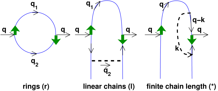
B.5 Distance dependence of angular correlations
B.5.1 Interaction diagrams
We focus now on the low-wavevector regime where the melt can be considered as incompressible (at least in terms of thermal blobs) and assume a Flory-distributed bath of a given inverse mean chain length . The corresponding results for infinite chains may be obtained by setting . The bond-bond correlation function is obtained by averaging over all intrachain pairs of bonds and at a given distance irrespective of their curvilinear distance . Setting thus for the Laplace variable conjugated to , the summed up Fourier-Laplace propagator becomes according to Eq. (29)
| (203) |
Using Eq. (60) and Eq. (63) the effective interaction potential thus reads WJO10
| (204) |
on large scales and . The momentum inserted in the interaction diagrams shown in Fig. 49 is conjugated to the distance between both bonds. Momentum is a conserved quantity flowing from one correlated point to the other. The wavevector associated with the first bond at the origin is called , the wavevector through the second bond . As may be better seen from the sketch included in Fig. 27, the first bond is now within the -subchain while the second bond is chosen to be outside. Putting both bonds within the subchain leads to trivial correlations even for Gaussian chains, putting both bonds outside the subchain leads to a vanishing correlation for as already remarked in Footnote 38 for the correlation function ANS10a . The first two diagrams in Fig. 49 for closed rings and linear chains are given by the convolution integrals
| (205) | |||||
| (206) |
We remind that for closed cycles the bond-bond correlation function does not vanish even for perfect Gaussian statistics and it is the corresponding zero order average which is computed by the first integral. The minus sign in front of the second integral for linear chains stems from the minus sign implied by the first order perturbation, Eq. (57). Using Eq. (82) and assuming Eq. (204) the integrals simplify considerably
| (207) | |||||
| (208) |
Using the well-known theorem for the (inverse) Fourier transformation of convolutions and that , the inverse Fourier transforms are thus
| (209) | |||||
| (210) |
with being the probability distribution to find another monomer of the chain around a reference monomer as given by Eq. (30). Interestingly, up to a constant prefactor the integrals and are thus equal on large scales ().
B.5.2 Normalization and bond-bond correlations
Focusing from now on the 3D case the bond-bond correlation function of closed rings is obtained from after normalization with . Using Eq. (30) this yields
| (211) |
with comparing the distance to the typical (-averaged) size of Flory-distributed chains. The reason for the normalization factor is that for both bonds are known to be bonds of the same polymer ring while the interaction integral Eq. (205) corresponds only to a probability for both bonds being in the same chain times a probability that this chain is closed. That is negative is of course due to the closure constraint which corresponds to an entropic spring force bending the second bond back to the origin. For large chain lengths the factor can be neglected and the bond-bond correlation function becomes a scale-free power law.
For linear chains it follows immediately from Eq. (210) that
| (212) |
being the limit for asymptotically long chains and using the scaling function for the finite- corrections. The normalization factor is due to the fact that for both bonds are known to belong to the same chain while the interaction integral Eq. (206) corresponds only to a probability for both bonds to be on the same chain. As compared to the closed cycles the correlation has the opposite sign since the attractive spring of the ring closure indicated by in Eq. (207) has been replaced by the effective repulsion indicated by in Eq. (208). This repulsion bends the second bond away from the origin increasing thus the bond-bond correlation function.
B.5.3 Sum rule and geometrical interpretation
Interestingly, the perturbation result, Eq. (209), for Flory-distributed chains may be rewritten as
| (213) |
where we have used the normalization factors mentioned above. This “sum rule” suggests a geometrical interpretation of the observed relation between infinite linear chains and closed cycles which may remain valid beyond the one-loop approximation used here.929292A similar sum rule is obtained for the bond-bond correlation function as a function of arc-length . One verifies readily that and thus with and being the density of chains of length in a Flory-distributed bath which would return after steps to the origin. This is the most elegant way to demonstrate that . The idea is that in an hypothetical ideal melt containing both linear chains and closed cycles all correlations disappear (on distances much smaller than the typical chain sizes) when summed up over the contributions of both architectures. The weight corresponds to the fraction of bond pairs in closed loops.939393Note that is the density of the monomers of both strands the reference monomer is connected to. We know for linear chains as for cycles that both bonds are connected by a first strand. The probability for both bonds to be in a closed loop is given by the density of the second strand. The factor is thus needed to avoid counting the same ring twice. Since the orientational correlations in ideal cycles are necessarily long-ranged due the ring closure (Eq. 211), it follows, assuming the sum rule, that the same applies to bond pairs of linear chains. Since bonds in closed cycles are anti-correlated (), they must be aligned () for linear chains. Interestingly, if one turns the argument around assuming the sum rule (rather than deriving it as we did) this imposes Eq. (204) and, hence, the effective intrachain potential for a Flory-distributed linear chain bath.
B.5.4 Finite chain size effects for Flory-distributed chains
We emphasize that the diagram shown in Fig. 49 is not sufficient to characterize for larger distances since the last diagram corresponding to the convolution integral
| (214) |
provides, as we shall see, the actual cutoff of the power law in this limit. Using again Eq. (82) and Eq. (204) the integral factorizes
| (215) | |||||
| (216) |
where we have introduced in the last line the convenient dimensionless constant
| (217) |
in which we dump local physics at large wavevector . Before evaluating the angular correlations in real space it is important to clarify the physics described by the diagram. The underlined second factor in Eq. (215) characterizes the alignment of the bond vectors of the monomers and at a fixed distance of the monomers and as shown by the sketch included in Fig. 27. Obviously, even for Gaussian chains these two bonds become more and more aligned if the distance gets larger than , i.e. when the chain segment becomes stretched. For perfectly Gaussian chains the bonds and at and would still remain uncorrelated, however, since the second bond is outside the chain segment on which we have imposed the distance constraint. As indicated by the dashed line in the diagram, it is then due to the effective interaction between the monomers within the stretched segment () and the monomers outside () that the bonds at and get aligned and then in turn the two bonds at and . We note that, strictly speaking, depends on the mean chain length , since is a function of . However, one checks readily that this effect can be neglected for reasonable mean chain lengths. We also note that the constant is finite, since the UV divergence which formally arises for large (where ) may be regularized by local and, hence, model dependent physics.949494For soft melts with weak bare excluded volume , i.e. , it can be shown that an upper cutoff wavevector regularizes the integral over . The coefficient becomes . Using and for this gives . This is not that far off the best fit value considering that for small one expects to be rather determined by the model-depending stiffness between adjacent bonds. We determine numerically from our simulations of self-assembled linear EP in Sec. 5.4.2.
Assuming a finite and chain length independent coefficient in Eq. (216) and inserting the propagator Eq. (203) we obtain by inverse Fourier transformation
| (218) |
for the interaction integral in real space. Normalizing as before with and summing over both diagrams for linear chains this yields
| (219) |
for . Comparing both terms in Eq. (219) one verifies that a crossover occurs at in agreement with Eq. (124) stated in the main text. The bond-bond correlation function of an incompressible solution of Flory distributed polymers becomes thus constant for . This remarkable result is essentially due to the polydispersity. This allows to find for all distances pairs of bonds and stemming from segments which are slightly stretched by an energy of order and which are, hence, slightly shorter than a unstretched segment of length . Since there are more shorter chains and chain segments this just compensates the decay of the weight due to the weak stretching. Although the number of such slightly stretched segments decays strongly with distance, their relative effect with respect to the typical unstretched segments, , remains constant for all . It is for this reason that the chemical potential appears in the second term of Eq. (219). Please note that bond pairs from strongly stretched segments (corresponding to an energy much larger than ) are, however, still exponentially suppressed and can be neglected. As explained in detail in Ref. WJO10 , this is qualitatively different for monodisperse chains where strongly stretched chain segments contribute increasingly to the average for large distances.
B.6 Non-extensivity of the chemical potential
We take again as a reference for the perturbation calculation a melt of Gaussian chains where the bond length is set by the effective bond length of asymptotically long chains. Averages performed over this unperturbed reference system are labeled by an index . The task is now to compute the ratio of the perturbed to the unperturbed partition function of the test chain of length plugged into the bath of -chains,
| (220) |
with the perturbation potential being the sum of the effective monomer interactions of all pairs of monomers of the test chain. The factor in Eq. (220) counts the number of equivalent monomer pairs separated by an arc-length . The deviation from Flory’s hypothesis is then given by the contribution to which is non-linear in . The calculation of Eq. (220) in dimensions is most readily performed in Fourier-Laplace space with being the wavevector conjugated to the monomer distance and the Laplace variable conjugated to the chain length . The Laplace transformed averaged perturbation potential reads
| (221) |
where represents the Fourier-Laplace transformed Gaussian propagator as given in Eq. (28) and the weight factor accounts again for the combinatorics between the interaction monomers — just as in Eq. (192).
The effective interaction potential being given by Eq. (59) one realizes that the naive perturbation calculation using Eq. (221) is formally diverging at high wavevectors in three dimensions (becoming only regular below ). This is due to monomer self-interactions which must be first subtracted. Using Eq. (64) instead of Eq. (59) even makes things worse due to an additional divergency associated with the self-interactions of the blobs whose size was set to zero (). However, since we are not interested in (possibly diverging) contributions linear in the length of the test chain or independent of it, we can freely subtract linear terms (i.e., terms in Laplace space) or constant terms (i.e., terms ) to regularize and to simplify . Such a transformation leads to
| (222) |
where “” stands for the linear and constant contributions we do not compute. This converges now for incompressible melts in dimensions. Applying Eq. (222) to incompressible Flory-distributed melts, i.e. assuming Eq. (40), this yields
| (223) | |||||
| (224) |
where we have read Eq. (223) as an inverse Fourier transform taken at . Remembering that a factor in -space stands for an integral in -space, the inverse Laplace transform of can be expressed in terms of integrals of the return probability . We obtain, hence, in -space
| (225) |
where stands for the non-extensive contribution to . Note that the first term in the brackets scales as the correlation hole in dimension. Its marginal dimension is . The second term characterizes the effective two-body interaction of the test chain with itself. As one expects DegennesBook , its marginal dimension is . Although Eq. (225) is formally obtained for it applies to higher dimensions by analytic continuation. In three dimensions Eq. (225) becomes
| (226) |
which demonstrates finally the non-extensive correction to the ideal polymer chain chemical potential announced in Eq. (108) and represented by the solid lines in Fig. 18. The chemical potential for monodisperse chains is obtained from Eq. (108) within the Padé approximation, Eq. (37), where is replaced by . This result is indicated by the dash-dotted lines in Fig. 18. A more precise calculation for monodisperse chains using the full Debye function is given in Ref. WJC10 .
References
- (1) P.M. Chaikin, T.C. Lubensky, Principles of condensed matter physics (Cambridge University Press, 1995)
- (2) P.J. Flory, Statistical Mechanics of Chain Molecules (Oxford University Press, New York, 1988)
- (3) P.G. de Gennes, Scaling Concepts in Polymer Physics (Cornell University Press, Ithaca, New York, 1979)
- (4) M. Doi, S.F. Edwards, The Theory of Polymer Dynamics (Clarendon Press, Oxford, 1986)
- (5) J. Higgins, H. Benoît, Polymers and Neutron Scattering (Oxford University Press, Oxford, 1996)
- (6) J. des Cloizeaux, G. Jannink, Polymers in Solution : their Modelling and Structure (Clarendon Press, Oxford, 1990)
- (7) L. Schäfer, Excluded Volume Effects in Polymer Solutions (Springer-Verlag, New York, 1999)
- (8) M. Rubinstein, R. Colby, Polymer Physics (Oxford University Press, Oxford, 2003)
- (9) F. Oozawa, S. Asakura, Thermodynamics in the Polymerization of Proteins (Academic, New York, 1975)
- (10) T. Witten, , P.A. Pincus, Structured Fluids: Polymers, Colloids, Surfactants (Oxford University Press, Oxford, 2004)
- (11) J.K.G. Dhont, An Introduction to Dynamics of Colloids (Elsevier, Amsterdam, 1996)
- (12) A.N. Semenov, J.F. Joanny, A. Khokhlov, Macromolecules 28, 1066 (1995)
- (13) F. Clément, A. Johner, J.F. Joanny, A. Semenov, Macromolecules 33, 6148 (2000)
- (14) M. Rubinstein, A. Semenov, Macromolecules 34, 1058 (2001)
- (15) P.J. Morris, Polymer Pioneers: A Popular History of the Science and Technology of Large Molecules (University of Pennsylvania Press, Philadelphia, 1989)
- (16) Y. Furukawa, Inventing polymer science: Staudinger, Carothers, and the emergence of macromolecular chemistry (University of Pennsylvania Press, Philadelphia, 1998)
- (17) M. Cates, S. Candau, J. Phys. Cond. Matt 2, 6869 (1990)
- (18) A.N. Semenov, S.P. Obukhov, J. Phys.: Condens. Matter 17, 1747 (2005)
- (19) B. Mandelbrot, The Fractal Geometry of Nature (W.H. Freeman, San Francisco, California, 1982)
- (20) J.N. Israelachvili, Intramolecular and Surface Forces (Academic Press, 1991)
- (21) C. Vanderzande, Lattice Models of Polymers (Cambridge University Press, Cambridge, 2004)
- (22) M. Allen, D. Tildesley, Computer Simulation of Liquids (Oxford University Press, Oxford, 1994)
- (23) J. Thijssen, Computational Physics (Cambridge University Press, Cambridge, 1999)
- (24) D. Frenkel, B. Smit, Understanding Molecular Simulation – From Algorithms to Applications (Academic Press, San Diego, 2002). 2nd edition
- (25) K. Binder, D. Herrmann, Monte Carlo Simulation in Statistical Physics: An Introduction, Fifth Edition (Springer, Heidelberg, 2002)
- (26) D.P. Landau, K. Binder, A Guide to Monte Carlo Simulations in Statistical Physics (Cambridge University Press, Cambridge, 2000)
- (27) W. Krauth, Statistical Mechanics: Algorithms and Computations (Oxford University Press, Oxford, U.K., 2006)
- (28) I. Carmesin, K. Kremer, Macromolecules 21, 2819 (1988)
- (29) J. Baschnagel, J.P. Wittmer, H. Meyer, in Computational Soft Matter: From Synthetic Polymers to Proteins, vol. 23, ed. by N. Attig (NIC Series, Jülich, 2004), vol. 23, pp. 83–140
- (30) M. Müller, in Handbook of Materials Modeling, ed. by S. Yip (Springer, Netherlands, 2005)
- (31) Q. Wang, J. Chem. Phys. 131, 234903 (2009)
- (32) A. Kron, Polym. Sci. USSR 7, 1361 (1965)
- (33) F. Wall, F. Mandel, J. Chem. Phys. 63, 4592 (1975)
- (34) F.A. Escobedo, J.J. de Pablo, J. Chem. Phys. 102, 2636 (1994)
- (35) P. Polanowski, T. Pakula, J. Chem. Phys. 117, 4022 (2002)
- (36) N. Karayiannis, A. Giannousaki, V. Mavrantzas, D. Theodorou, J. Chem. Phys. 117, 5465 (2002)
- (37) B.J. Banaszak, J.J. de Pablo, J. Chem. Phys. 119, 2456 (2003)
- (38) P.J. Flory, J. Chem. Phys. 13, 453 (1945)
- (39) P.J. Flory, J. Chem. Phys. 17, 303 (1949)
- (40) S. Edwards, Proc. Phys. Soc. 85, 613 (1965)
- (41) S. Edwards, Proc. Phys. Soc. 88, 265 (1966)
- (42) S. Edwards, J.Phys.A: Math.Gen. 8, 1670 (1975)
- (43) M. Muthukumar, S. Edwards, J. Chem. Phys. 76, 2720 (1982)
- (44) M. Abramowitz, I.A. Stegun, Handbook of Mathematical Functions (Dover, New York, 1964)
- (45) T. Lodge, N. Rotstein, S. Prager, Adv. Chem. Phys. 79, 1 (1990)
- (46) A.N. Semenov, in Theoretical Challenges in the Dynamics of Complex Fluids, ed. by T. McLeish (Kluwer, Dordrecht, 1997), pp. 63–86
- (47) A.N. Semenov, M. Rubinstein, Eur. Phys. J. B 1, 87 (1998)
- (48) J.M. Deutsch, Phys. Rev. Lett. 54, 56 (1985)
- (49) L. Mattioni, J.P. Wittmer, J. Baschnagel, J.L. Barrat, E. Luijten, Eur. Phys. J. E 10, 369 (2003)
- (50) W. Paul, K. Binder, D. Heermann, K. Kremer, J. Phys. II 1, 37 (1991)
- (51) W. Paul, K. Binder, D. Heermann, K. Kremer, J. Chem. Phys. 95, 7726 (1991)
- (52) J.P. Wittmer, W. Paul, K. Binder, Macromolecules 25, 7211 (1992)
- (53) J.P. Wittmer, W. Paul, K. Binder, Journal de Physique II 4, 873 (1994)
- (54) J.S. Shaffer, J. Chem. Phys. 101, 4205 (1994)
- (55) J.S. Shaffer, J. Chem. Phys. 103, 761 (1995)
- (56) T. Kreer, J. Baschnagel, M. Müller, K. Binder, Macromolecules 34, 1105 (2001)
- (57) K. Hagita, H. Takano, J. Phys. Soc. Jpn. 72, 1824 (2003)
- (58) G.S. Grest, K. Kremer, Phys. Rev. A 33, 3628 (1986)
- (59) K. Kremer, G. Grest, J. Chem. Phys. 92, 5057 (1990)
- (60) S.J. Plimpton, J. Comp. Phys. 117, 1 (1995)
- (61) J.T. Padding, W.J. Briels, J. Chem. Phys. 114, 8685 (2001)
- (62) J.T. Padding, W.J. Briels, J. Chem. Phys. 117, 925 (2002)
- (63) R. Everaers, S. Sukumaran, G. Grest, C. Svaneborg, A. Sivasubramanian, K. Kremer, Science 303, 823 (2004)
- (64) H. Meyer, T. Kreer, A. Cavallo, J.P. Wittmer, J. Baschnagel, Eur. Phys. J. Special Topics 141, 167 (2007)
- (65) Q. Wang, Y. Yin, J. Chem. Phys. 130, 104903 (2009)
- (66) B. Dünweg, J. Chem. Phys. 99, 6977 (1993)
- (67) P. Ahlrichs, R. Everaers, B. Dünweg, Phys. Rev. E 64, 040501 (2001)
- (68) N. Spenley, Europhys. Lett. 49, 534 (2000)
- (69) E. Nikomarov, S. Obukhov, Sov. Phys. JETP 53, 328 (1981)
- (70) J. Curro, K. Schweizer, G. Grest, K. Kremer, J. Chem. Phys. 91, 1359 (1991)
- (71) M. Müller, K. Binder, L. Schäfer, Macromolecules 33, 4568 (2000)
- (72) Z.G. Wang, J. Chem. Phys. 117, 481 (2002)
- (73) R. Auhl, R. Everaers, G. Grest, K. Kremer, S. Plimpton, J. Chem. Phys. 119, 12718 (2003)
- (74) D. Shirvanyants, S. Panyukov, Q. Liao, M. Rubinstein, Macromolecules 1, 1475 (2008)
- (75) D. Morse, J. Chung, J. Chem. Phys. 130, 224901 (2009)
- (76) J. Qin, D. Morse, J. Chem. Phys. 130, 224902 (2009)
- (77) W. Paul, G.D. Smith, D.Y. Yoon, B. Farago, S. Rathgeber, A. Zirkel, L. Willner, D. Richter, Phys. Rev. Lett. 80, 2346 (1998)
- (78) G. Smith, W. Paul, M. Monkenbusch, D. Richter, Chemical Physics 261, 61 (2000)
- (79) W. Paul, G. Smith, Rep. Prog. Phys. 67, 1117 (2004)
- (80) J.P. Wittmer, H. Meyer, J. Baschnagel, A. Johner, S.P. Obukhov, L. Mattioni, M. Müller, A.N. Semenov, Phys. Rev. Lett. 93, 147801 (2004)
- (81) J.P. Wittmer, P. Beckrich, F. Crevel, C.C. Huang, A. Cavallo, T. Kreer, H. Meyer, Comp. Phys. Comm. 177, 146 (2007)
- (82) J.P. Wittmer, P. Beckrich, A. Johner, A.N. Semenov, S.P. Obukhov, H. Meyer, J. Baschnagel, Europhys. Lett. 77, 56003 (2007)
- (83) P. Beckrich, A. Johner, A.N. Semenov, S.P. Obukhov, H.C. Benoît, J.P. Wittmer, Macromolecules 40, 3805 (2007)
- (84) J.P. Wittmer, P. Beckrich, H. Meyer, A. Cavallo, A. Johner, J. Baschnagel, Phys. Rev. E 76, 011803 (2007)
- (85) H. Meyer, J.P. Wittmer, T. Kreer, P. Beckrich, A. Johner, J. Farago, J. Baschnagel, Eur. Phys. E 26, 25 (2008)
- (86) J.P. Wittmer, A. Cavallo, T. Kreer, J. Baschnagel, A. Johner, J. Chem. Phys. 131, 064901 (2009)
- (87) J.P. Wittmer, A. Johner, S.P. Obukhov, H. Meyer, A. Cavallo, J. Baschnagel, Macromolecules 43, 1621 (2010)
- (88) J.P. Wittmer, A. Johner, A. Cavallo, P. Beckrich, F. Crevel, J. Baschnagel, Eur. Phys. J. E 31, 229 (2010)
- (89) A. Semenov, Macromolecules 43, 9139–9154 (2010)
- (90) J. Wittmer, P. Polińska, A. Cavallo, H. Meyer, J. Farago, A. Johner, J. Baschnagel, J. Chem. Phys. 134, 234901 (2011)
- (91) J. Farago, H. Meyer, A. Semenov, A. Johner, J. Wittmer, J. Baschnagel, Phys. Rev. E (2011). Submitted.
- (92) J. Farago, H. Meyer, A. Semenov, Phys. Rev. Lett. (2011). Submitted.
- (93) J. Farago, H. Meyer, J. Baschnagel, A. Semenov, Phys. Rev. E (2011). Submitted.
- (94) A.N. Semenov, A. Johner, Eur. Phys. J. E 12, 469 (2003)
- (95) A. Cavallo, M. Müller, J.P. Wittmer, A. Johner, K. Binder, J. Phys.: Condens. Matter 17, S1697 (2005)
- (96) N. Lee, J. Farago, H. Meyer, J. Wittmer, J. Baschnagel, S. Obukhov, A. Johner, EPL 96, 48002 (2011)
- (97) J.P. Wittmer, N. Schulmann, P. Polińska, A. Cavallo, J. Farago, J. Chem. Phys. (2011). In preparation.
- (98) A. Kolinski, J. Skolnick, R. Yaris, J. Chem. Phys. 86, 1567, 7164, 7174 (1987)
- (99) M. Guenza, Phys. Rev. Lett. 88, 025901 (2002)
- (100) M. Doxastakis, D. Theodorou, G. Fytas, F. Kremer, R. Faller, F. Müller-Plathe, N. Hadjichristidis, J. Chem. Phys. 119, 6883 (2003)
- (101) G. Logotheti, D. Theodorou, Macromolecules 40, 2235 (2007)
- (102) R. Scott, J. Phys. Chem. 69, 261 (1965)
- (103) J. Wheeler, S. Kennedy, P. Pfeuty, Phys. Rev. Lett. 45, 1748 (1980)
- (104) G. Faivre, J. Gardissat, Macromolecules 19, 1988 (1986)
- (105) Y. Rouault, A. Milchev, Phys. Rev. E 51, 5905 (1995)
- (106) J.P. Wittmer, A. Milchev, M.E. Cates, Europhys. Lett. 41, 291 (1998)
- (107) J.P. Wittmer, A. Milchev, M.E. Cates, J. Chem. Phys. 109, 834 (1998)
- (108) A. Milchev, in Computational methods in colloid and interface science, ed. by M. Borowko, M. Dekker (New York, 2000), p. 510
- (109) C.C. Huang, H. Xu, F. Crevel, J. Wittmer, J.P. Ryckaert, in Computer Simulations in Condensed Matter: from Materials to Chemical Biology, vol. 704 (Springer, Lect. Notes Phys., International School of Solid State Physics, Berlin/Heidelberg, 2006), vol. 704, pp. 379–418
- (110) M. Kröger, R. Makhloufi, Phys. Rev. E 53, 2531 (1996)
- (111) J. Padding, E. Boek, Phys. Rev. E 66, 756 (2004)
- (112) I.Y. Erukhimovich, A.N. Semenov, Sov. Phys. JETP 28, 149 (1986)
- (113) A.N. Semenov, S. Anastiadis, N. Boudenne, G. Fytas, M. Xenidou, N. Hadjichristidis, Macromolecules 30, 6280 (1997)
- (114) F. Brochard, P.G. de Gennes, J. de Phys. Lett. 40, L399 (1979)
- (115) S.P. Obukhov, A.N. Semenov, Phys. Rev. Lett. 95, 038305 (2005)
- (116) N.G. van Kampen, Stochastic processes in physics and chemistry (North-Holland, Amsterdam, 1992)
- (117) D. Chandler, Introduction to Modern Statistical Mechanics (Oxford University Press, New York, 1987)
- (118) H. Meyer, N. Schulmann, J.E. Zabel, J.P. Wittmer, Comp. Phys. Comm. 182, 1949 (2011)
- (119) H. Meyer, T. Kreer, M. Aichele, A. Cavallo, A. Johner, J. Baschnagel, J.P. Wittmer, Phys. Rev. E 79, 050802(R) (2009)
- (120) H. Meyer, J.P. Wittmer, T. Kreer, A. Johner, J. Baschnagel, J. Chem. Phys. 132, 184904 (2010)
- (121) M. Müller, J.P. Wittmer, M.E. Cates, Phys. Rev. E 61, 4078 (2000)
- (122) T. Vettorel, A. Grosberg, K. Kremer, Phys. Biol. 6, 025013 (2009)
- (123) F. Eurich, P. Maass, J. Chem. Phys. 114, 7655 (2001)
- (124) C. Likos, Physics Reports 348, 267 (2001)
- (125) D. Wu, G. Fredrickson, J.P. Carton, A. Ajdari, L. Leibler, J. Poly. Sci.: Part B: Polymer Physics 33, 2373 (1995)
- (126) H.P. Wittmann, K. Kremer, Comp. Phys. Comm. 61, 309 (1990)
- (127) H. Deutsch, R. Dickman, J. Chem. Phys. 93, 8983 (1990)
- (128) H. Deutsch, K. Binder, J. Chem. Phys. 94, 2294 (1991)
- (129) M. Müller, W. Paul, J. Chem. Phys. 100, 719 (1994)
- (130) N. Wilding, M. Müller, J. Chem. Phys. 101, 4324 (1994)
- (131) A. Rubio, J. Lodge, J. Freire, Macromolecules 35, 5295 (2002)
- (132) M. Müller, J.P. Wittmer, M.E. Cates, Phys. Rev. E 53, 5063 (1996)
- (133) M. Müller, J.P. Wittmer, J.L. Barrat, Europhys. Lett. 52, 406 (2000)
- (134) M. Müller, EPFL Supercomputing Review 7, 21 (1995)
- (135) M. Müller, Macromol. Theory Simul. 8, 343 (1999)
- (136) A. Cavallo, M. Müller, K. Binder, Europhys. Lett. 61, 214 (2003)
- (137) A. Cavallo, M. Müller, K. Binder, J. Phys. Chem. B 109, 6544 – 6552 (2005)
- (138) S. Kamath, R. Colby, S. Kumar, Macromolecules 36, 8567 (2003)
- (139) J.U. Sommer, K. Saalwächter, Eur. Phys. J. E 18, 167 (2005)
- (140) K. Okun, M. Wolfgardt, J. Baschnagel, K. Binder, Macromolecules 30, 3075 (1997)
- (141) K. Binder, J. Baschnagel, W. Paul, Prog. Polym. Sci. 28, 115 (2003)
- (142) M. Molina-Mateo, J. Meseguer-Duenas, J. Gomez-Ribelles, Polymer 46, 7463 (2005)
- (143) J. Freire, J. of Physics-Condensed Matter 20, 285102 (2008)
- (144) M. Arnoult, J. Saiter, C. Pareige, J. Duenas, J. Ribelles, J. Mateo, J. Chem. Phys. 130, 214905 (2009)
- (145) A. Werner, F. Schmid, M. Müller, J. Chem. Phys. 110, 5370 (1999)
- (146) J. Luettmer-Strathmann, F. Rampf, W. Paul, K. Binder, J. Chem. Phys. 128, 064903 (2008)
- (147) J. Wittmer, A. Johner, J.F. Joanny, K. Binder, J. Chem. Phys. 101, 4379 (1994)
- (148) A. Kopf, J. Baschnagel, J. Wittmer, K. Binder, Macromolecules 29, 1433 (1996)
- (149) J.P. Wittmer, M.E. Cates, A. Johner, M.S. Turner, Europhys. Lett. 33, 397 (1996)
- (150) P. Khalatur, A. Khokhlov, S. Prokhorova, S. Sheiko, M. Möller, P. Reineker, D. Shirvanyanz, Eur. Phys. J. E 1, 99 (2000)
- (151) C. Mischler, J. Baschnagel, K. Binder, Adv. Coll. Interf. Sci. 94, 197 (2001)
- (152) M. Müller, J. Chem. Phys. 116, 9930 (2002)
- (153) C. Mischler, J. Baschnagel, S. Dasgupta, K. Binder, Macromolecules 43, 467 (2002)
- (154) A. Cavallo, J. Wittmer, A. Johner, J. Baschnagel, J. Chem. Phys. (2011). In preparation.
- (155) A. Cavallo, M. Müller, K. Binder, Macromolecules 39, 9539 (2006)
- (156) A. Cavallo, M. Müller, K. Binder, Macromolecules 41, 4937 (2008)
- (157) R.P. Feynmann, R. Leighton, Surely you’re joking, Mr. Feynman (W. W. Norton, New York, 1985)
- (158) P. van der Schoot, J.P. Wittmer, Macromolekuare Theory and Simulations 8, 428 (1999)
- (159) A. Milchev, J.P. Wittmer, D.P. Landau, Phys. Rev. E 61, 2959 (2000)
- (160) J.P. Wittmer, M. Milchev, P. van der Schoot, J.L. Barrat, J. Chem. Phys. 113, 6992 (2000)
- (161) M. Szwarc, Nature 178, 1168 (1956)
- (162) B. O’Shaughnessy, J. Yu, Phys. Rev. Lett. 74, 4329 (1995)
- (163) D.A. McQuarrie, Statistical Mechanics (University Science Books, Sausalito, California, 2000)
- (164) I. Yerukhimovich, Polymer Science U.S.S.R 19, 2743 (1977)
- (165) K. Shimomura, H. Nakanishi, N. Mitarai, Phys. Rev. E 80, 051804 (2009)
- (166) K.C. Daoulas, M. Müller, J. Chem. Phys. 125, 184904 (2006)
- (167) M. Rawiso, R. Duplessix, C. Picot, Macromolecules 20, 630 (1987)
- (168) S. Gagliardi, V. Arrighi, R. Ferguson, A.C. Dagger, J.A. Semlyen, J.S. Higgins, J. Chem. Phys. 122, 064904 (2005)
- (169) J. Hansen, I. McDonald, Theory of simple liquids (Academic Press, New York, 1986)
- (170) M. Fuchs, K. Kroy, J. Phys.: Condens. Matter 14, 9223 (2002)
- (171) M.H.J. Hagen, I. Pagonabarraga, C.P. Lowe, D. Frenkel, Phys. Rev. Lett. 78, 3785 (1997)
- (172) S. Williams, G. Bryant, I. Snook, W. van Megen, Phys. Rev. Lett. 96, 087801 (2006)
- (173) T. Bauer, F. Höfling, T. Munk, E. Frey, T. Franosch, Eur. Phys. J. Special Topics 189, 103 (2010)
- (174) J.P. Wittmer, A. Johner, S.P. Obukhov, P. Polińska, O. Benzerara, H. Meyer, J. Baschnagel, Eur. Phys. E (2011). In preparation.
- (175) K. Schweizer, J. Chem. Phys. 91, 5802 (1989)
- (176) S. Chong, A. Aichele, H. Meyer, M. Fuchs, J. Baschnagel, Phys. Rev. E 76, 051806 (2007)
- (177) J.P. Wittmer, H. Meyer, A. Johner, T. Kreer, J. Baschnagel, Phys. Rev. Lett. 105, 037802 (2010)
- (178) B. Duplantier, J. Stat. Phys. 54, 581 (1989)
- (179) C. Svaneborg, G. Grest, R. Everaers, Europhys. Lett. 72, 760 (2005)
- (180) M. Müller, G.D. Smith, J. Polym. Sci. B: Polymer Physics 43, 934 (2005)
- (181) E. Meyer, R. Overney, K. Dransfeld, T. Gyalog, Nanoscience: Friction and Rheology on the Nanometer Scale (World Scientific, Singapore, 1998)
- (182) B. Frank, A. Gast, T. Russel, H. Brown, C. Hawker, Macromolecules 29, 6531 (1996)
- (183) R. Jones, S. Kumar, D. Ho, R. Briber, T. Russel, Nature 400, 146 (1999)
- (184) B. Maier, J.O. Rädler, Phys. Rev. Lett. 82, 1911 (1999)
- (185) S. Granick, S. Kumar, E. Amis, et al., J. Polym. Sci. B 41, 2755 (2003)
- (186) K. Shin, H. Xiang, S. Moon, T. Kim, T. MacCarthy, T. Russel, Science 306, 76 (2004)
- (187) P. O’Connell, G. McKenna, Science 307, 1760 (2005)
- (188) G.T. Gavranovic, J.M. Deutsch, G.G. Fuller, Macromolecules 38, 6672 (2005)
- (189) F. Sun, A. Dobrynin, D. Shirvanyants, H. Lee, K. Matyjaszewski, G. Rubinstein, M. Rubinstein, S. Sheiko, Phys. Rev. Lett. 99, 137801 (2007)
- (190) K. Shin, S. Obukhov, J.T. Chen, J. Huh, Y. Hwang, S. Mok, P. Dobriyal, P. Thiyagarjan, T. Russell, Nature Materials 6, 961 (2007)
- (191) E. Eisenriegler, Polymers near surfaces (World Scientific, Singapore, 1993)
- (192) J.L. Jacobson, N. Read, H. Saleur, Phys. Rev. Lett. 90, 090601 (2003)
- (193) Y. Ikhlef, J.L. Jacobson, H. Saleur, J. Stat. Mech. - Theory and Experiment May, P05005 (2007)
- (194) P.Z. Wong, A.J. Bray, Phys. Rev. Lett. 60, 1344 (1988)
- (195) J.D. Halverson, W. Lee, G. Grest, A. Grosberg, K. Kremer, J. Chem. Phys. 134, 204904 (2011)
- (196) M. Cates, J. Deutsch, J. Phys. 47, 2121 (1986)
- (197) S. Obukhov, M. Rubinstein, T. Duke, Phys. Rev. Lett. 73, 1263 (1994)
- (198) K. Hur, R.G. Winkler, D.Y. Yoon, Macromolecules 39, 3975 (2006)
- (199) J. Suzuki, A. Takano, T. Deguchi, Y. Matsushita, J. Chem. Phys. 131, 144902 (2009)
- (200) K. Hur, C. Jeong, R. Winkler, N. Lacevic, R. Gee, D. Yoon, Macromolecules 44, 2311 (2011)
- (201) G.B. West, J.H. Brown, B.J. Enquist, Science 284, 1677 (1999)
- (202) A. Milchev, Eur. Phys. J. E 8, 531 (2002)
- (203) D. Ermak, J. Chem. Phys. 62, 4189 (1975)
- (204) R. Groot, P. Warren, J. Chem. Phys. 107, 4423 (1997)
- (205) A.N. Semenov, Phys. Rev. Lett. 80, 1908 (1998)