Determining the wavelength of Langmuir wave packets at the Earth’s bow shock

Abstract

The propagation of Langmuir waves in plasmas is known to be sensitive to density fluctuations. Such fluctuations may lead to the coexistence of wave pairs that have almost opposite wave-numbers in the vicinity of their reflection points. Using high frequency electric field measurements from the WIND satellite, we determine for the first time the wavelength of intense Langmuir wave packets that are generated upstream of the Earth’s electron foreshock by energetic electron beams. Surprisingly, the wavelength is found to be 2 to 3 times larger than the value expected from standard theory. These values are consistent with the presence of strong inhomogeneities in the solar wind plasma rather than with the effect of weak beam instabilities.

1 Introduction

The theory of beam-plasma interactions in homogeneous plasmas is one of the pillars of plasma physics, and yet it fails to properly describe some important physical phenomena observed, such as the generation of type III solar radio bursts or waves registered in the electron foreshock region, upstream of the Earth’s bow shock (Ginzburg, 1970; Robinson, 1997). The major reason for this discrepancy between observations and the theory of quasilinear, weak or strong turbulence is supposed to be related to the existence of strong density fluctuations that are not associated with the beams. When these fluctuations are large enough, Langmuir waves can be trapped or reflected and in both cases the wave-vector $\vec{k}_{1}$ of the reflected wave becomes approximately equal and opposite to that of the incident wave $\vec{k}_{0}\simeq-\vec{k}_{1}$. Such strong density fluctuations are not resolved by existing particle detectors. However, they provide a useful means for inferring the wavelength, which is difficult to measure directly in space plasmas.

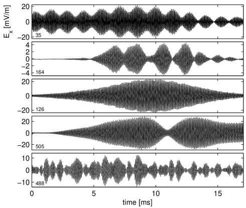
The WAVES instrument (Bougeret et al., 1995) onboard the WIND satellite routinely measures Langmuir waves at high time resolution (up to 120 000 samples per second) in the solar wind. When two large amplitude and counter-propagating waves coexist, a monochromatic wave packet with a slowly varying envelope is produced. Some typical examples are shown in Fig. 1. Here, for the first time, we show how the wavelength of these waves can be directly estimated from a polarization analysis of two components of the electric field. Interestingly, the measured value disagrees with estimates derived from standard beam-plasma theory in homogeneous plasmas but is consistent with estimates derived for strongly inhomogeneous plasmas.

2 The effect of density fluctuations

Density fluctuations in the solar wind plasma have been studied for many years (Neugebauer, 1975; Celnikier et al., 1987) and exhibit a power law over many decades. The smallest scales are difficult to measure by lack of time resolution and counting statistics of standard particle instruments. Recently, Ergun et al. (2008) observed the interaction of density fluctuations with Langmuir waves, and described them as eigenmodes trapped inside density depletions. In such strongly inhomogeneous plasmas, wave propagation is strongly affected by density fluctuations. As a consequence, the dynamics of the instability departs quite substantially from that observed in homogeneous plasmas (Nishikawa and Riutov, 1976; Muschietti et al., 1985; Krasnoselskikh et al., 2007). Such density inhomogeneities can cause high frequency electrostatic waves to be converted into electromagnetic waves (Bale et al., 1998; Kellogg et al., 1999). They also affect the statistics of wave amplitudes (Cairns et al., 2000; Krasnoselskikh et al., 2007) and the presence of sufficiently large inhomogeneities eventually leads to wave reflection (Ginzburg, 1970; Budden, 1988).

Figure 1: Five typical coherent Langmuir wave packets observed by WIND. Only the $E_{\rm x}$ electric field component is shown. The bottom plot shows a marginal case in which the wave-packet is barely coherent.

Here, we focus on the dynamics of Langmuir waves that are generated near the electron foreshock edge region by electron beams with a typical energy of 1–3 keV (Filbert and Kellogg, 1979). These waves have a narrowband spectrum and their characteristic frequency is close to the electron plasma frequency. The presence of relatively large but slowly varying (with respect to the wavelength) density fluctuations, with

$$\delta n/n_{0}\gg\frac{3}{2}k^{2}\lambda_{\rm D}^{2}$$ (1)

can substantially alter the beam-plasma instability by changing the wave-vector $\vec{k}$ along the trajectory of the beam. Here, $\vec{k}$ is the wave-vector of the plasma wave, $n_{0}$ the background plasma density and $\lambda_{\rm D}$ is the Debye length. The wave trajectory in the inhomogeneous plasma can be described by the equations

$$\frac{d\vec{r}}{dt} = \frac{\partial\omega}{\partial\vec{k}}$$ (2)

$$\frac{d\vec{k}}{dt} = -\frac{\partial\omega}{\partial\vec{r}}$$ (3)

that results in a $\vec{k}$-vector change with the density that is described by

$$\vec{k}\;\lambda_{\rm D}=\sqrt{\frac{2}{3\omega_{p}}\left[\omega-\omega_{p}\frac{\delta n(x)}{2n_{0}}\right]}$$ (4)

The observations we present hereafter clearly show the simultaneous presence of two oppositely propagating waves with $\vec{k}$-vectors close to each other, so that $\vec{k}_{1}\approx-\vec{k}_{0}$. Two scenarios can lead to such a coexistence of primary and oppositely directed secondary waves. The first one is the scattering off of density fluctuations, and the second one is three-wave decay.

Let us consider the first scenario. Without loss of generality, we assume here that the density increases along the x direction. In this case, the $k_{\rm x}$ component of the wave-vector and the wave group velocity both decrease along x. The wave amplitude then increases even in the absence of growth or damping. This effect can be illustrated in the WKB approximation, where the solution of the wave equation can be written in the form

$$E\sim E_{0}\sqrt{\frac{k_{0{\rm x}}}{k_{\rm x}\left({\rm x}\right)}}\exp\left(-j\omega t+j\int k_{\rm x}({x})\;dx\right),$$ (5)

and the amplitude increases when $k_{\rm x}\left({x}\right)$ decreases. Without damping or growth, the component of the energy flux $F$ along the density gradient can be supposed to be constant. We then have $F\sim V_{\rm gr}E^{2}\sim k_{\rm x}E^{2}=$ const and so the wave amplitude $E$ scales like $k_{\rm x}^{-1/2}$. In the WKB approximation, reflection processes are supposed to be similar to mirroring, with part of the energy being reflected and part damped. Two large amplitude waves, incident and backscattered, can thus be observed simultaneously in the vicinity of the reflection point (Bale et al., 2000). It is worth mentioning that the WKB approximation is valid close to, but not at, the turning point where $k_{\rm x}$ goes to zero. Immediately near this point the wave amplitude resembles solutions of the Schrödinger equation with a linearly varying potential expressed in terms of Airy functions and it remains finite at the reflection point (see Sect. 17 in Ginzburg, 1970).

The second scenario is a change in the characteristics of the wave-wave interaction by a variation of the wave-vector. The growth of primary waves generated by beam-plasma interactions can be saturated by the decay process $l_{0}\rightarrow l_{1}+s$, in which a primary Langmuir wave $l_{0}$ decays into a secondary Langmuir wave $l_{1}$ and an ion-sound wave $s$. The threshold condition for the decay instability is

$$\frac{\varepsilon_{0}E_{0}^{2}}{2n_{0}k_{B}T}>\frac{\nu_{\rm S}\nu_{\rm L}}{\omega_{\rm S}\omega_{\rm L}}.$$ (6)

Here, $E_{0}$ is the amplitude of the primary wave, $T$ is the electron temperature, $\nu_{\rm S}$ and $\nu_{\rm L}$ are respectively the damping rates of the secondary ion sound and Langmuir waves, and $\omega_{\rm S}$ and $\omega_{\rm L}$ are their pulsations. When the primary wave propagates into a denser plasma, the decrease in $k_{\rm x}$ leads to a decrease of the wave-vector of the secondary waves. The phase velocity of the secondary Langmuir wave then grows and the damping rate drops, finally initiating a decay instability. It is well known from linear theory that the maximum increment of decay instability then corresponds to almost exact back scatter with a small correction to comply with momentum and energy conservation laws. As a consequence, in this case the wave-vector $\vec{k}_{1}$ of the secondary Langmuir wave becomes also approximately equal and opposite to that of the primary wave, i.e. $\vec{k}_{1}\approx-\vec{k}_{0}$.

These oppositely-directed waves provide a unique opportunity for measuring their wavelength without requiring multipoint measurements.

3 Expressions for evaluating the wavelength

We assume that the frequency difference $\delta f=f_{0}-f_{1}$ (where $f_{0}$ and $f_{1}$ are respectively the frequencies of the incident and reflected waves) is mainly caused by the Doppler shift rather than by the frequency difference associated with the differing dispersions of the two waves. Indeed, this frequency difference significantly exceeds that of the ion-sound wave that might be generated by the decay process. In the spacecraft reference frame, the wave frequencies are

$$f_{l}=f_{p}\left(1+\frac{3}{2}k_{l}^{2}\lambda_{\rm D}^{2}\right)+\frac{\vec{k}_{l}\cdot\vec{V}_{\rm SW}}{2\pi}~{}~{}l=0,1$$ (7)

where ${V}_{\rm SW}$ is the velocity of the plasma with respect to satellite. We assume that

$$\frac{\vec{k}_{l}\cdot\vec{V}_{\rm SW}}{\omega_{p}}\gg\frac{3}{2}{k}_{l}^{2}\lambda_{\rm D}^{2},$$ (8)

and will check this a posteriori. Theoretical predictions and observations both lend support to the alignment of the wave-vector of the primary (and consequently secondary) waves along the magnetic field. Since the two wave-vectors have almost equal magnitudes, we find

$$\delta f=f_{0}-f_{1}\simeq\frac{2\vec{k}_{0}\cdot\vec{V}_{\rm SW}}{2\pi}=\frac{\vec{k}_{0}}{\pi}\left(\frac{\vec{B}}{B}\cdot\vec{V}_{\rm SW}\right),$$ (9)

where we suppose that both wave-vectors are approximately co-aligned with the magnetic field. From this expression, we finally obtain the wavelength $\lambda=2\pi/{k}_{0}$. Let us now show how these different quantities are estimated.

Figure 2: Analysis procedure of a typical wave packet: (a) two components of the electric field in GSE coordinates, (b) identification of the two peaks in the power spectral density (continuous curves are gaussian fits), (c) verification that the amplitudes and the phases (not shown) indeed vary slowly in time, (d) hodogram to compare the polarisation with the orientation of the magnetic field. The direction of the solar wind velocity varies and is not necessarily aligned with the magnetic field.

4 Determining the wavelength in practice

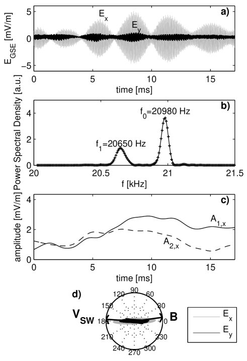
In practice, to measure the wavelength of the wave packets, we first need to know their direction of propagation, which is a prerequisite for estimating the wave-vector $\vec{k}$. We first convert the electric field components into Geocentric Solar Ecliptic (GSE) coordinates, hence defining components $E_{\rm x}$ and $E_{\rm y}$, see Fig. 2a. Next, a continuous Fourier transform is applied in a small interval around the plasma frequency. Except for some distorted wave-packets whose modulation width $T$ is only a few oscillation periods, the power spectral density usually exhibits two distinct peaks, see Fig. 2b. The relative width $\Delta f/f$ (where $\Delta f$ is the full width at half maximum) of these peaks is always well below 1%, confirming the stability of the frequency over the interval. Each component of the electric field can then be modeled as a sum of two complex exponentials. A least-squares regression of the following model is performed

$$E_{i}(t) = A_{0,i}(t)\,{\rm Re}\left[\exp{\left(j2\pi f_{0}t+j\phi_{0,x}(t)\right)}\right]$$

$$+ A_{1,i}(t)\,{\rm Re}\left[\exp{\left(j2\pi f_{1}t+j\phi_{1,i}(t)\right)}\right]$$

$$+ C_{i}(t)+\epsilon_{i}(t)$$

where $i=x$ or $y$ and $\epsilon(t)$ is the residual error to be minimized. The amplitude $A(t)$ and the phase $\phi(t)$ vary slowly with respect to $T$. Possible offsets are taken care of by a small and slowly varying constant $C(t)$. We use a sliding gaussian window of width $W$ to estimate these parameters at different parts of the wave-packet. Obviously, we must have $1/f_{0}\ll W\ll T$. Taking $W=10/f_{0}$ was found to be a good compromise. We checked that the amplitudes $A_{0}(t)$ and $A_{1}(t)$ show no beating like the original wave packets do (Fig. 2c) and that the phases $\phi_{0}(t)$ and $\phi_{1}(t)$ indeed vary slowly with respect to the wave period.

Once the amplitudes and the phases are known, we can separate the components of the electric field corresponding to the primary and secondary waves. A plot in polar coordinates (see Fig. 2d) reveals their polarisation in the xy-plane. Also shown are the projection on that plane of the magnetic field $\vec{B}$ and the solar wind velocity $\vec{V}_{\rm SW}$. For electrostatic waves, $\nabla\cdot\vec{E}=0\Rightarrow\vec{k}\,/\!/\,\vec{E}$ and so the direction of the wave-vector $\vec{k}$ should be given by the semi-major axis of the polarisation ellipse.

Figure 2d shows two remarkable results, which are systematically found for all the coherent wave-packets we analyzed. First, both waves are almost linearly polarized and their polarisation ellipses have the same orientation. We conclude that their wave-vectors are necessarily parallel or antiparallel, as expected. Secondly, the angle between the semi-major axis of the polarisation ellipse and the ambient magnetic field is always small, rarely exceeding 20$\deg$. The absence of the third $E_{\rm z}$ component in principle prevents us from concluding that $\vec{k}\,/\!/\,\vec{B}$. For all the events we analyzed, however, we always found the polarisation ellipse to be parallel to the magnetic field, no matter how the latter is oriented. We therefore conclude that both waves must necessarily propagate along or very close to the magnetic field direction. Momentum conservation finally implies $\vec{k}_{0}\approx-\vec{k}_{1}$.

Figure 3: Example of electric field spectrum from the WAVES instrument (top plot) and electron flux from the Three-Dimensional Plasma and Energetic Particle Investigation (Lin et al., 1995) on 17 April 1996.

For the example shown in Fig. 2, we measure $\delta f=330$ Hz, $f_{p}=20.815$ kHz and so from Eq. (9) we finally obtain the wavelength $\lambda=2.57$ km. We check that the waves are indeed weakly dispersive, since from Eq. (8) we have

$$\frac{\vec{k}\cdot\vec{V}_{\rm SW}}{\omega_{p}}=0.017\gg\frac{3}{2}{k}^{2}r_{\rm D}^{2}=0.0031$$ (10)

Similar values are obtained for the other coherent wave packets shown in Fig. 1, except for the last one, for which $f_{0}$ and $f_{1}$ cannot be properly identified. We analyzed 644 wave-packets that way and found the wavelength to be on average $\lambda=2.1$ km, with a standard deviation of 0.5 km; the typical Debye length in the solar wind at 1 AU is 10 m.

5 Discussion and conclusion

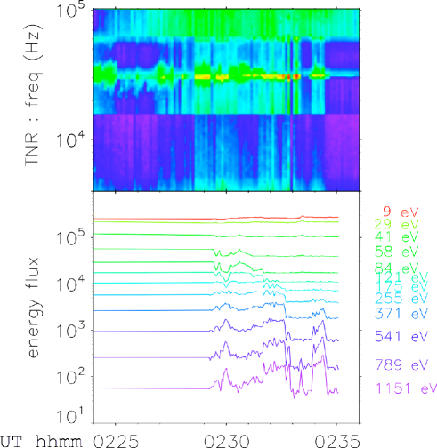
The coherent wave packets we observe always coincide with an enhancement in the energetic electron flux. The energy of these electrons ranges from several hundreds of eV up to several keV. Figure 3 shows the energetic electron flux measured by WIND during a typical burst of Langmuir wave activity. Fitzenreiter et al. (1996) have shown that these wave packets are associated with bump on tail features in the electron distribution. Their wavelength then should be $\lambda=2\pi V_{\rm b}/\omega_{p}$, where $V_{\rm b}$ is the beam velocity. For waves with a frequency of 20 kHz that are generated by 1 keV electron beams, we find $\lambda=935$ m. This value is about 2.3 times smaller than the one we measure. The two values cannot be reconciled by assuming that the wave activity is triggered by higher energy energy electrons, since unrealistic energies in excess of 5 keV would be required.

The wavelength we observe, however, is compatible with that found for wave propagation in inhomogeneous plasma. As it was pointed out by Kellogg et al. (1999) from the analysis of the density fluctuation spectra, variations in the $\vec{k}$-vector, as caused by density fluctuations, can exceed the vector magnitude. Therefore, the discrepancy we observe between the predicted and observed wavelengths is most probably due to a change of the wave-vector when the waves propagate into a higher density region. Indeed, for the solar wind conditions we consider, the variation of the wave dispersion can be as large as

$$\delta\omega/\omega_{p}=(3/2)k^{2}\lambda_{\rm D}^{2}\ \approx\ 0.3\%.$$ (11)

The associated level of density variations is

$$\delta n/n\ \approx\ 2\delta\omega/\omega_{p}\ \approx\ 0.6\%.$$ (12)

Such levels are compatible with estimates made at the electron foreshock (Neugebauer, 1975; Celnikier et al., 1987; Kellogg et al., 1999) and are large enough to offer an explanation for the relatively large wavelengths we observe.

Our conclusion is further supported by recent direct observations by Ergun et al. (2008) and Krasnoselskikh et al. (2007) of unusually high levels of density fluctuations in the solar wind. The conventional theory of beam-plasma interaction that has been developed for homogeneous plasmas does not apply to such cases. Indeed, our results show in an unambiguous way that the observed wavelengths exceed their theoretical prediction. The theory should therefore include the effect of large amplitude random density fluctuations from the very beginning.

Acknowledgements

V. K. acknowledges CNES for financial support through Scientific Space Research Proposal entitled “Cluster Co-I DWP”.
     Guest Editor M. Gedalin thanks one anonymous referee for her/his help in evaluating this paper.

The publication of this article is financed by CNRS-INSU.

References

- Bale et al. (1998) Bale, S. D., Kellogg, P. J., Goetz, K., and Monson, S. J.: Transverse Z-mode waves in the terrestrial electron foreshock, Geophys. Res. Lett., 25, 9–12, 1998.
- Bale et al. (2000) Bale, S. D., Larson, D. E., Lin, R. P., Kellogg, P. J., Goetz, K., and Monson, S. J.: On the beam speed and wavenumber of intense electron plasma waves near the foreshock edge, J. Geophys. Res., 105, 27353–27368, doi:10.1029/2000JA900042, 2000.
- Bougeret et al. (1995) Bougeret, J.-L., Kaiser, M. L., Kellogg, P. J., Manning, R., Goetz, K., Monson, S. J., Monge, N., Friel, L., Meetre, C. A., Perche, C., Sitruk, L., and Hoang, S.: Waves: The Radio and Plasma Wave Investigation on the Wind Spacecraft, Space Sci. Rev., 71, 231–263, doi:10.1007/BF00751331, 1995.
- Budden (1988) Budden, K. G.: The Propagation of Radio Waves, Cambridge University Press, Cambridge, 1988.
- Cairns et al. (2000) Cairns, I. H., Robinson, P. A., and Anderson, R. R.: Thermal and driven stochastic growth of Langmuir waves in the solar wind and Earth’s foreshock, Geophys. Res. Lett., 27, 61–64, doi:10.1029/1999GL010717, 2000.
- Celnikier et al. (1987) Celnikier, L. M., Muschietti, L., and Goldman, M. V.: Aspects of interplanetary plasma turbulence, Astron. Astrophys., 181, 138–154, 1987.
- Ergun et al. (2008) Ergun, R. E., Malaspina, D. M., Cairns, I. H., Goldman, M. V., Newman, D. L., Robinson, P. A., Eriksson, S., Bougeret, J. L., Briand, C., Bale, S. D., Cattell, C. A., Kellogg, P. J., and Kaiser, M. L.: Eigenmode Structure in Solar-Wind Langmuir Waves, Phys. Rev. Lett., 101, 051101, doi:10.1103/PhysRevLett.101.051101, 2008.
- Filbert and Kellogg (1979) Filbert, P. C. and Kellogg, P. J.: Electrostatic noise at the plasma frequency beyond the earth’s bow shock, J. Geophys. Res., 84, 1369–1381, doi:10.1029/JA084iA04p01369, 1979.
- Fitzenreiter et al. (1996) Fitzenreiter, R. J., Vinas, A. F., Klimas, A. J., Lepping, R. P., Kaiser, M. L., and Onsager, T. G.: Wind observations of the electron foreshock, Geophys. Res. Lett., 23, 1235–1238, 1996.
- Ginzburg (1970) Ginzburg, V. L.: The propagation of electromagnetic waves in plasmas, Pergamon, Oxford, 2nd edn., 1970.
- Kellogg et al. (1999) Kellogg, P. J., Goetz, K., Monson, S. J., and Bale, S. D.: Langmuir waves in a fluctuating solar wind, J. Geophys. Res., 104, 17069–17078, doi:10.1029/1999JA900163, 1999.
- Krasnoselskikh et al. (2007) Krasnoselskikh, V. V., Lobzin, V. V., Musatenko, K., Souček, J., Cairns, I., and Pickett, J.: Beam-plasma interaction in randomly inhomogeneous plasmas and statistical properties of small-amplitude Langmuir waves in the solar wind and electron foreshock, J. Geophys. Res, 112, A10109, doi:10.1029/2006JA012212, 2007.
- Lin et al. (1995) Lin, R. P., Anderson, K. A., Ashford, S., Carlson, C., Curtis, D., Ergun, R., Larson, D., McFadden, J., McCarthy, M., Parks, G. K., Rème, H., Bosqued, J. M., Coutelier, J., Cotin, F., D’Uston, C., Wenzel, K.-P., Sanderson, T. R., Henrion, J., Ronnet, J. C., and Paschmann, G.: A Three-Dimensional Plasma and Energetic Particle Investigation for the Wind Spacecraft, Space Sci. Rev., 71, 125–153, doi:10.1007/BF00751328, 1995.
- Muschietti et al. (1985) Muschietti, L., Goldman, M. V., and Newman, D.: Quenching of the beam-plasma instability by large-scale density fluctuations in 3 dimensions, Sol. Phys., 96, 181–198, 1985.
- Neugebauer (1975) Neugebauer, M.: The enhancement of solar wind fluctuations at the proton thermal gyroradius, J. Geophys. Res., 80, 998–1002, 1975.
- Nishikawa and Riutov (1976) Nishikawa, K. and Riutov, D. D.: Relaxation of relativistic electron beam in a plasma with random density inhomogeneities, J. Phys. Soc. Jpn., 41, 1757–1765, 1976.
- Robinson (1997) Robinson, P. A.: Nonlinear wave collapse and strong turbulence, Rev. Mod. Phys., 69, 507–573, doi:10.1103/RevModPhys.69.507, 1997.