A modified star formation law as a solution to open problems in galaxy evolution

Abstract

In order to reproduce the low mass end of the stellar mass function, most current models of galaxy evolution invoke very efficient supernova feedback. This solution seems to suffer from several shortcomings however, like predicting too little star formation in low mass galaxies at z=0. In this work, we explore modifications to the star formation (SF) law as an alternative solution to achieve a match to the stellar mass function. This is done by applying semi-analytic models based on De Lucia & Blaizot, but with varying SF laws, to the Millennium and Millennium-II simulations, within the formalism developed by Neistein & Weinmann. Our best model includes lower SF efficiencies than predicted by the Kennicutt-Schmidt law at low stellar masses, no sharp threshold of cold gas mass for SF, and a SF law that is independent of cosmic time. These simple modifications result in a model that is more successful than current standard models in reproducing various properties of galaxies less massive than $10^{10}{\rm M}_{\odot}$. The improvements include a good match to the observed auto-correlation function of galaxies, an evolution of the stellar mass function from $z=3$ to $z=0$ similar to observations, and a better agreement with observed specific star formation rates. However, our modifications also lead to a dramatic overprediction of the cold mass content of galaxies. This shows that finding a successful model may require fine-tuning of both star formation and supernovae feedback, as well as improvements on gas cooling, or perhaps the inclusion of a yet unknown process which efficiently heats or expels gas at high redshifts.

1 Introduction

Ever since first introduced by White & Frenk (1991), semi-analytic models of galaxy formation and evolution (hereafter SAM; Kauffmann et al., 1999; Kang et al., 2005; Croton et al., 2006; Bower et al., 2006; Cattaneo et al., 2006; De Lucia & Blaizot, 2007; Monaco et al., 2007; Somerville et al., 2008; Khochfar & Silk, 2009) have been successfully used to study how different physical processes determine the formation and evolution of galaxies. Based on halo merger trees extracted from $N$-body simulations or analytic methods, SAMs follow the main processes that are thought to affect the properties of galaxies, like gas cooling, star formation, feedback, and merging. These models provide a useful tool to study the interplay and the relative importance of these different physical processes. A detailed review of the semi-analytic method can be found in Baugh (2006).

Although various observational properties of galaxies are matched by the models, current SAMs still have problems in reproducing some important observations and up to now, there is no semi-analytic model that is able to fit all the key statistical properties of the observed galaxy population. For example, Guo et al. (2011) show that the model of De Lucia & Blaizot (2007) substantially overproduces the low mass end of the stellar mass function of galaxies. This problem becomes more severe as the resolution of the underlying dark matter simulation increases. In addition, stellar mass functions at high redshifts are normally not well reproduced (Fontanot et al., 2009; Marchesini et al., 2009); a good match to the 2-point auto-correlation function of galaxies is so far difficult to achieve (e.g. Guo et al., 2011); and the relation between the specific star formation rate and galaxy stellar mass deviates from observations (Somerville et al., 2008; Fontanot et al., 2009).

These discrepancies may have various reasons: inaccurate physical modeling of the processes that govern galaxy formation; technical problems in tuning the model against a large set of observational constraints; the use of a fixed functional form for a poorly understood process, which overly limits the freedom in tuning the model; or a wrong cosmological model adopted in the simulations. This large range of possibilities makes it difficult to correct identified discrepancies between model and observations.

For example, Guo et al. (2011) tried to fix the over-prediction of the low mass end of the stellar mass function, as modeled by De Lucia & Blaizot (2007), by increasing the effect of supernovae feedback. They managed to reproduce the amplitude of galaxy stellar mass function, and also obtained a reasonable match to the galaxy luminosity functions in different bands. However, they also predict a too large fraction of red galaxies at low masses, too high amplitudes of the stellar mass functions in the redshift range of [0.8, 2.5], and galaxy auto-correlation functions that are too high for galaxies less massive than $6\times 10^{10}{\rm M}_{\odot}$. Moreover, the high feedback efficiency as used by Guo et al. (2011) is physically difficult to motivate (Benson et al., 2003), and is far more efficient than various solutions adopted by hydrodynamical simulations (Mac Low & Ferrara, 1999; Strickland & Stevens, 2000; Avila-Reese et al., 2011).

In this work, we therefore explore an alternative solution. We tune the SF recipe instead of the supernovae (SN) feedback to study how our changes affect different statistics of galaxies, and to what degree the discrepancies mentioned above can be alleviated. Most of the current SAMs use an analogue to the empirical Kennicutt–Schmidt law (Schmidt, 1959; Kennicutt, 1998) to calculate the star formation rate (SFR) in galaxies. In this standard prescription, the SFR is roughly proportional to the cold gas mass, and scales inversely with the typical time-scale of a galactic disk (e.g. Cole et al., 2000). This law is combined with a sharp threshold at low gas densities, below which no SF occurs (Kauffmann, 1996; Croton et al., 2006). The use of a such a threshold is motivated both theoretically (e.g. Toomre, 1964; Kennicutt, 1989; Schaye, 2004) and observationally (e.g. Martin & Kennicutt, 2001).

This simple SF law is however likely an oversimplification. In recent years observational determinations of the SF law in galaxies have become increasingly refined, using various gas components (HI, CO) in combination with more reliable estimates of SF, based on UV and IR light. These recent findings can be summarized as follows: First, there are indications that the threshold for SF at low mass densities is not sharp. Instead, the SF efficiency drops off as a steep power-law at low gas densities (Kennicutt et al., 2007; Bigiel et al., 2008; Wyder et al., 2009; Roychowdhury et al., 2009; Bigiel et al., 2010). Second, several studies find that the SF rate is correlated more strongly with the mass of molecular gas (H₂) than with the the atomic gas (Wong & Blitz, 2002; Bigiel et al., 2008; Leroy et al., 2008), probably also at high redshift (Bouché et al., 2007; Genzel et al., 2010). This shows that simply correlating the star formation rate with the total cold gas density in models may not always lead to realistic results. It is also not clear which gas mass correlates best with the SF rate when averaging over the entire galaxy (e.g. Saintonge et al., 2011). Third, there are both theoretical and observational indications that the normalization of the SF law might be lower at high redshift than locally (e.g. Wolfe & Chen, 2006; Rafelski et al., 2010; Gnedin & Kravtsov, 2010; Agertz et al., 2011; Krumholz & Dekel, 2011). This means that simply extrapolating the local relation, as done in most SAMs, may be incorrect.

Several recent models have attempted to address these issues. Baugh et al. (2005), Weinmann et al. (2011a), and Krumholz & Dekel (2011) specifically lower the quiescent star formation efficiencies at high redshifts in order to better match some observed properties of high redshift galaxies. Both Fu et al. (2010) and Lagos et al. (2010, 2011) focus on the first two of the above points, and present SAMs with updated and much more detailed SF recipes in comparison to previous SAMs. They do not include a sharp threshold for SF, and their SF rate depends on the molecular gas density instead of on the cold gas mass, following recent empirical and theoretical models (e.g. Blitz & Rosolowsky, 2006; Krumholz et al., 2009). Their detailed models for SF depend on various internal properties of the disk, like size and pressure, which are not trivial to model in a SAM.

It is certainly worthwhile to try and include more detailed and observationally and theoretically better motivated SF law into SAMs. We present a complementary approach in this work, without taking into account complicated processes on sub-galactic scales, like the conversion from atomic to molecular gas. We instead try to solve in a straightforward way the inverse problem, namely which realistic SF law at galactic scales is required to improve the agreement between model galaxies and observations. We start with a standard model, similar to De Lucia & Blaizot (2007) and Neistein & Weinmann (2010), and assume that the SF rate depends on the cold gas mass in the galaxy, cosmic time, and in addition the host halo mass. We make simple change to the standard SF law that are qualitatively, but not quantitatively plausible, and explore how those impact on the properties of galaxies. We show that we can improve the agreement between SAMs and observations in several key aspects in this way.

We use the model developed by Neistein & Weinmann (2010), and implement it on both the Millennium Simulation (MS, Springel et al., 2005) and the Millennium-II Simulation (MS-II, Boylan-Kolchin et al., 2009). The properties of galaxies with masses as low as $\sim$ $10^{8}{\rm M}_{\odot}$ can probably be studied reliably with the help of these simulations (Guo et al., 2011), although this can be resolution dependent for extreme models (see Neistein & Weinmann 2010). Our aim is to investigate how much a model based on De Lucia & Blaizot (2007) can be changed and improved by tuning the SF law alone. We thus do not change gas cooling and feedback in our models, but leave it at the default standard values (except in one case, for illustration, as will be explained).

This paper is organized as follows. In section 2 we present the different models used in this work. Our starting point is a model that is based on the widely used SAM of De Lucia & Blaizot (2007), with an improved prescription for hot gas stripping of satellite galaxies. We then develop four different models. Of these, models 2 and 3 include the key changes to the quiescent and burst mode star formation. In section 3 we present predictions for the stellar mass functions at low and high redshifts, the relation between galaxy specific SF rate and stellar mass, the galaxy cold gas mass function, the auto-correlation functions, and the SF rate density as a function of redshift. A discussion of the implications of our results, and the conclusions are presented in section 4.

2 models

The semi-analytic models presented in this paper are applied to both the MS and MS-II simulations. The cosmological parameters in the simulations are consistent with a combined analysis of the 2dFGRS (Colless et al., 2001) and the first year WMAP data (Spergel et al., 2003), with $\Omega_{\rm m}=0.25$, $\Omega_{\rm b}=0.045$, $h=0.73$, $\Omega_{\Lambda}=0.75$, $n=1$, and $\sigma_{8}=0.9$. Note that these parameters are different from the latest WMAP 7 year results. Both simulations follow $N=2160^{3}$ particles from redshift $z=127$ to the present day. The MS has a particle mass resolution of $8.6\times 10^{8}\,h^{-1}{\rm M}_{\odot}$, with a comoving box of $500\,h^{-1}$Mpc on a side. The MS-II has a mass resolution of $6.9\times 10^{6}\,h^{-1}{\rm M}_{\odot}$, with a box of side $100\,h^{-1}$Mpc.

Neistein & Weinmann (2010) (hereafter NW2010) developed a new formalism for modeling galaxy formation and evolution, which is similar to the standard SAMs, except that the efficiencies of processes like gas cooling, star formation and feedback are assumed to depend only on the host halo mass and cosmic time. NW2010 have shown that this new method produces a very similar population of galaxies like standard SAMs. The method is simple and flexible, which makes it easy to change recipes in order to fit selected observational constraints.

All the models within this work are based on a simple set of differential equations, that follow the mass of gas and stars within galaxies. We adopt the model of De Lucia & Blaizot (2007, hereafter DLB07) as our starting point, as was done in NW2010. The reader is referred to these papers, and to Croton et al. (2006), for more details on the model assumptions. Here we highlight a few features that will be important for the discussion below. The SF law is assumed to be:

$${\dot{M}_{\rm star}}={f_{s}}(M_{\rm cold}-M_{\rm crit})$$ (1)

$f_{s}$ is the SF efficiency in units of Gyr^-1, and $M_{\rm crit}$ is the critical mass of cold gas, below which no star formation occurs (Kennicutt, 1998). Satellite galaxies are followed along with their host subhaloes. Once the subhaloes are stripped and cannot be identified anymore, we compute the radial distance, $r_{\rm sat}$, between the satellite and the central subhalo within the group. We then allow the satellite galaxy to spiral in further, and estimate the time it merges into the central object by using dynamical friction estimate:

$$t_{\rm df}=\alpha_{\rm df}t_{\rm C}=\alpha_{\rm df}\frac{1.17V_{\rm v}r_{\rm sat}^{2}}{GM_{1}\ln\left(1+M_{\rm h}/M_{1}\right)}\,.$$ (2)

Here $t_{\rm C}$ is the Chandrasekhar estimate for the dynamical friction timescale, where $V_{\rm v}$ is the virial velocity of the central subhalo, $M_{\rm h}$ is its mass, and $M_{1}$ is the baryonic (cold gas and stellar) mass of the satellite galaxy. $\alpha_{\rm df}$ describes the ratio of the adopted dynamical friction time over the Chandrasekhar estimate. When galaxies finally merge we assume a SF burst of the type:

$${\dot{M}_{\rm star,\rm burst}}={{\alpha}_{\rm burst}}{(M_{1,\rm cold}+M_{2,\rm cold})}\,,$$ (3)

with

$${\alpha_{\rm burst}}={0.56}(M_{1}/M_{2})^{0.7}\,.$$ (4)

Here $M_{1}$ and $M_{2}$ denote the baryonic mass in the merging galaxies. Following Croton et al. (2006), this formula is derived from fitting the results of hydrodynamical simulations (e.g. Cox et al., 2004, see section 2.4 for more details).

In the following subsections, we describe all the models used in this paper in detail.

2.1 Model 0

Our model 0) is very similar to model 0) in NW2010, and should thus be also similar to DLB07. For the SF law above (Eq. 1) we use the same fitting functions as in NW2010:

$$f_{s}=2.04\,M_{12}^{0.094}10^{-0.039[\log M_{12}]^{2}}t^{-0.82}\,,$$ (5)

and

$$M_{\rm crit}=0.36\,f_{s}^{-1}M_{12}^{0.68}t^{-0.52}\,.$$ (6)

Here $t$ is the Hubble time in units of Gyr, and $M_{12}=M_{\rm halo}/10^{12}$ is the halo mass in unit of $10^{12}h^{-1}{\rm M}_{\odot}$.

There are a few minor modifications made here in comparison to NW2010, that are related to the extended range in halo mass we use here (a minimum halo mass of $\sim 10^{8}$ h${}^{-1}\,M_{\odot}$ in comparison to $\sim 10^{10}$ h${}^{-1}\,M_{\odot}$ in NW2010). For more details on how we extend the recipes from NW2010 to low mass haloes, the reader is referred to Appendix A. Fig. 1 shows that the amplitude of the low mass end of the stellar mass function (SMF) for model 0) is comparable to the DLB07 result when applied to MS-II simulation.

2.2 Model 1

Model 1) is the fiducial model used in this work. It is based on model 0) as presented in the previous subsection, but includes two further changes: the hot gas stripping of satellite galaxies is slowed down considerably compared to DLB07 following Weinmann et al. (2010), and a larger dynamical friction time is assumed.

In the DLB07 model, the hot gas component of a galaxy is stripped completely once it falls into a larger group and becomes a satellite. Satellite galaxies subsequently consume their remaining cold gas due to star formation and efficient SN feedback, and the SF rate ceases on a short timescale of 1 - 2 Gyr. This leads to most satellite galaxies displaying red colour, which is in contradiction with observations (Wang et al., 2007; Weinmann et al., 2009). Following the model suggested by Weinmann et al. (2010), we assume in model 1) that the hot gas component of satellite galaxies decreases at the same rate as their surrounding dark matter haloes, which lose mass due to tidal stripping. This treatment provides a physically better motivated description of the behaviour of the hot gas component of satellite galaxies and improves agreement with observations (Weinmann et al., 2010). A similar model is included in the recent SAM of Guo et al. (2011).

The second change with respect to model 0) is that the parameter $\alpha_{\rm df}$, which describes the ratio of dynamical friction time for galaxy mergers over the Chandrasekhar formula (Eq. 2 above), is set to $5$, in contrast to the value $2$ as adopted in model 0) and in DLB07. This corresponds to a larger time scale for satellite galaxies to merge with the central galaxy, and is chosen in order to get auto-correlation functions in better agreement with observations for all the models (see below). Up to now there is no solid consensus on what $\alpha_{\rm df}$ should be in models (Boylan-Kolchin et al., 2008; Jiang et al., 2008; Mo et al., 2010).

Green lines in Fig. 1 show the SMF of the fiducial model 1), with dashed and solid lines for results when applied to MS and MS-II simulations. Model 1) SMF are in general slightly higher than model 0). This is mainly due to the slower stripping of hot gas in satellites adopted in model 1). Retaining their hot gas reservoir for longer, satellite galaxies can continue forming stars for a considerable time and thus end up with a higher stellar mass than in model 0). When merging into central galaxies, they also add more mass to their centrals. Although our choice of a larger dynamical friction time, with $\alpha_{\rm df}=5$, delays merger to some degree and thereby decreases the amount of mass added to centrals, this effect is apparently smaller than that of the modification to the hot gas stripping. When comparing results of model 0) and model 1) for the MS and MS-II simulations, the SMF in the MS exceed the SMF in the MS-II at intermediate masses. This is not the case for DLB07 (Guo et al., 2011). This excess may be related to the fact that our extension of the cooling efficiencies do not exactly match those used for DLB07 in Guo et al. (2011).

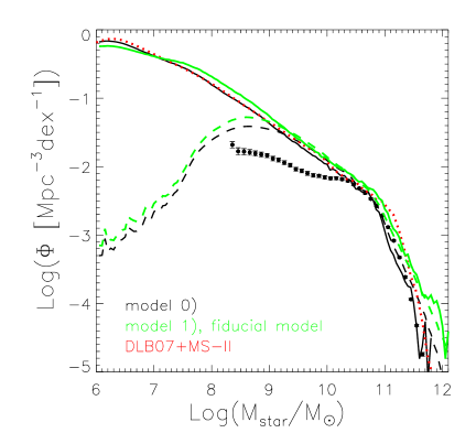
Figure 1: The stellar mass functions of model 0) (black lines) and the fiducial model 1) (green lines). Dashed lines are obtained using the MS simulation, and solid lines are for the MS-II simulation. The red dotted line shows the stellar mass function using the DLB07 SAM for MS-II simulation. Filled dots with error bars show the observed stellar mass function of SDSS DR7 result (Li & White, 2009; Guo et al., 2010).

2.3 Model 2

In model 2), we make modifications to the SF law in the quiescent mode, and keep all the other components of the model exactly the same as in the fiducial model 1). The modifications include: a) $M_{\rm crit}=0$, which means no threshold cold gas mass for SF; b) the SF efficiency depends more strongly on halo mass; c) the SF efficiency does not depend on the Hubble time.

The SF law in model 2) is chosen such that the low mass end slope of SMF in the model is comparable to the observed SDSS result, when applied to MS simulation. This results in

$$M_{\rm crit}=0\,,$$ (7)

$${f_{s}}=0.41\,{M_{12}^{0.94}10^{-0.30[\log M_{12}]^{2}}}\,.$$ (8)

Fig. 2 compares the SF efficiency (SFE, defined as the ratio between SF and the mass of the cold gas) in the quiescent mode in model 1) and model 2), as a function of halo mass at two redshifts. Green lines are efficiencies in model 1). Solid green lines are for a cold gas–halo mass ratio of $0.04$/$0.09$ at $z=0$/$z=3$, which corresponds to the median cold gas–halo mass ratio in model 1). Dashed green lines are for a higher cold gas–halo mass ratio of $0.13$/$0.14$ at $z=0$/$z=3$, and dotted green lines are for a lower ratio of $0.007$/$0.05$ at $z=0$/$z=3$. These values correspond to the 16th and 84th percentiles of the distributions in cold gas masses in model 1). The SF efficiency in model 2) is shown as red-blue lines, which follow a power law of index $2$ (plotted as black dotted lines in Fig. 2) for haloes less massive than $\sim 10^{11.5}h^{-1}{\rm M}_{\odot}$. Compared to model 1), model 2) has a lower SF efficiency at $z=0$ for halo masses between $10^{10}$ and $\sim 10^{11.5}h^{-1}{\rm M}_{\odot}$. At $z=3$, the SF efficiency is much lower in model 2) than in model 1) for haloes less massive than $\sim 10^{12}h^{-1}{\rm M}_{\odot}$.

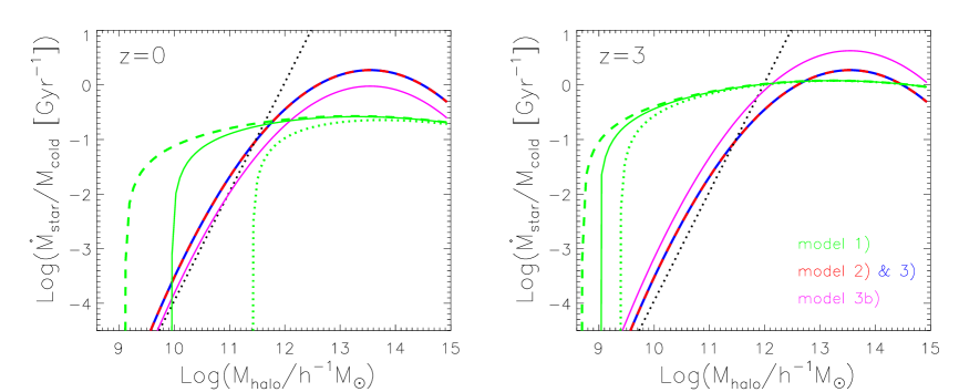
Figure 2: Star formation efficiencies in the quiescent mode as a function of halo mass at $z=0$ (left panel) and $z=3$ (right panel). Green lines are the efficiencies in model 1). Dashed, solid and dotted green lines are for the cases when the cold gas–halo mass ratios are [84, 50, 16] percentile values in model 1), which are [$0.13$, $0.04$, $0.007$] at $z=0$, and are [$0.14$, $0.09$, $0.05$] at $z=3$. Red-blue line is the efficiency of star formation for model 2) and 3). The magenta lines are for efficiencies in model 3b). Black dotted line shows a power law with index 2 for reference.

2.4 Model 3

When applying model 2) to the MS simulation, the amplitude of the SMF at the low mass end decreases dramatically and matches the observation of SDSS (red dashed line in Fig. 3). However, when applied to the MS-II simulation, the low mass end of SMF is still too high (red solid line in Fig. 3). We have tested that even when truncating all SF in quiescent disk mode in haloes less massive than $\sim 10^{11.5}h^{-1}{\rm M}_{\odot}$, the problem still exists. This is because galaxy mass grows not only by quiescent SF in disks, but also by merger-induced bursts. These become more significant if the quiescent SF efficiency is decreased, due to the resulting increase in the cold gas masses.

In model 3), we therefore further modify the SF law in the burst mode, while keeping the same SF law for the quiescent mode as in model 2). The star burst efficiency used in current SAMs (Eq. 4) is derived from fitting the results of hydrodynamical simulations for mergers of mass ratios ranging from 1:10 to 1:1 (Cox et al., 2004; Mihos & Hernquist, 1994, 1996). The parameters in those simulations are set to make the SF in an isolated disk galaxy consistent with the Kennicutt-Schmidt law. As the quiescent SF of dwarf galaxies themselves is lower than that predicted by the Kennicutt-Schmidt law, it is quite possible that those simulations over-predict the burst efficiency for low mass galaxies. Therefore we introduce a halo mass dependence for the efficiency of merger-induced bursts in model 3), and make it inefficient for low mass haloes.

For haloes less massive than $M_{0}$, we modify the burst efficiency to be

$${\alpha_{\rm burst}}={0.56}(M_{1}/M_{2})^{0.7}{\times}({M_{\rm halo}}/{M_{0}})\,.$$ (9)

while it remains unchanged for higher mass haloes. We use $M_{0}=10^{11.5}h^{-1}{\rm M}_{\odot}$. This critical halo mass is empirically determined, and roughly corresponds to the mass where the relation between galaxy stellar mass and halo mass changes its slope (e.g. Wang et al., 2006; Moster et al., 2010), and galaxy formation efficiency reaches its maximum (Guo et al., 2010). Physically, SN feedback and reionization are believed to cause a low galaxy formation efficiency at low halo masses, and AGN feedback may be responsible for the low efficiency in high mass haloes (Guo et al., 2010). The combined effect of these mechanisms may be weakest at this critical halo mass, explaining the peak in galaxy formation efficiency in the current theory. Therefore we choose this value as the threshold below which the SF efficiency is assumed to be suppressed. The typical stellar mass of galaxies that reside in those haloes is about $10^{10.5}{\rm M}_{\odot}$, below which model 0) and model 1) predict too many galaxies and thus too much SF. By decreasing the SF for galaxies with halo mass less massive than this critical value, the amplitude of the low mass end of the stellar mass function can be suppressed effectively. The functional form in Eq. 9 is chosen in order to fit the amplitude of the SMF at the low mass end when applied to both MS and MS-II simulation.

We have also tested a model in which we shut off all SF in the burst mode in low mass haloes and keep the SF in the quiescent mode the same as in the fiducial model 1). For such a model, the low mass end of the SMF is still higher than observation. This indicates that SF in both the quiescent and the burst mode must be modified simultaneously to suppress the numbers of low mass galaxies effectively. Note that the values of the power law indices that determine the dependence of SF on halo mass for quiescent and burst modes might have some degeneracy. However, we do not study the degeneracy of the two modes of SF in this work any further, but focus on the qualitative effect of modifying SF in each mode.

2.5 Model 3b

In model 3b), we test the effect of including a dependence of the SF efficiency on Hubble time. Model 3b) is almost identical to model 3), except that the SF efficiency in the quiescent mode is assumed to depend on cosmic time, in the same way as for the fiducial model 1). The SF efficiency is rescaled to match again the low mass end of SMF in SDSS observation, resulting in:

$${f_{s}}=1.74\,{M_{12}^{0.94}10^{-0.30[\log M_{12}]^{2}}}t^{-0.82}\,.$$ (10)

The SF efficiency in model 3b) is also shown in Fig. 2. It is higher than the SF efficiency in model 3) at high redshift, and is lower at $z=0$. We will see in the next section that compared with model 3), model 3b) results in a similar SMF at $z=0$, and higher amplitude of SMF at higher redshifts of $z\sim 2-3$. The lower SFR at redshift $0$ results in low mass galaxies with a lower SSFR than in model 3). Besides, model 3b) predicts a higher SFR density at redshifts higher than $\sim 2$, and a lower SFR density at lower redshifts. The general results are comparable with model 3) though.

2.6 Model 4

With a modified SF law in low mass haloes, model 3) and 3b) are able to reproduce many observational statistics of low mass galaxies, as we will show in in Sec. 3. However, the properties of high mass galaxies differ significantly from observations. The most obvious deviation is that the modeled massive galaxies are in general too active. This is mainly due to the inclusion of slower stripping of hot gas for satellite galaxies in our models. The deviation can be alleviated by allowing for less efficient cooling in massive haloes. Physically, this corresponds to mechanisms like stronger AGN feedback effect that prevents gas from cooling.

In model 4), we apply further modifications of cooling and SF to model 3), focusing on massive galaxies. Model 4) is presented as a simple test to see if the properties of massive galaxies can be better fitted, while keeping the the treatment of low mass galaxies unchanged. The modifications include:

• Lower cooling efficiencies are assumed for haloes more massive than $10^{11.75}h^{-1}{\rm M}_{\odot}$, as shown in Fig. 12 in the Appendix.

• SF in both the quiescent and the burst mode is stopped completely in haloes more massive than $5\times 10^{12}h^{-1}{\rm M}_{\odot}$ at $z<1.3$.

• The dynamical friction time is assumed to be dependent on Hubble time and is shorter at higher redshift, with $\alpha_{\rm df}=5\times(t/13.6)^{0.5}$ instead of $\alpha_{\rm df}=5$ in model 3) (see Weinmann et al., 2011a).

These modifications are done to fit the observed properties of massive galaxies better. The first two modifications make massive galaxies much more passive than in model 3). The change in the dynamical friction time follows the idea of Weinmann et al. (2011a). As discussed there, the merger time in the standard model may be overestimated by an order of magnitude at high redshift, mainly due to the more radial orbits of high redshift satellite galaxies (Dekel et al., 2009; Hopkins et al., 2010). Therefore we assume a time-dependent dynamical friction time, which gives a better fit to the SFR density and SMF at $z>2$, and does not affect the other statistics studied in this work much.

3 Results

In this section, we show statistical results for the galaxy population produced by the models presented in the last section, including galaxy SMF at both low and high redshifts, the specific SF rate–stellar mass relation, the cold gas mass function, the projected two point correlation functions, and SF rate density as a function of redshift. We compare these results with observations, and analyze the effect of different modifications of SF laws on those statistics.

3.1 Stellar mass function at $z=0$

The SMF at $z=0$ is the main quantity that was used to constrain the parameter values in our models, and is plotted in Fig. 3. Similar to previous SAMs (DLB07, Guo et al., 2011), the fiducial model 1) predicts too many low mass galaxies. As a result of the modifications in the SF law in low mass haloes, model 2) applied to the MS fits the SMF for stellar masses less massive than $10^{9.3}{\rm M}_{\odot}$. However, when applied to the MS-II, model 2) still predicts too many low mass galaxies. By suppressing the SF in the burst mode in low mass haloes, model 3) gives a reasonable fit to the observed SMF, for both MS and MS-II simulations. Including a dependence of the SF on cosmic time in model 3b) does not affect the SMF noticebly. For model 4) which changes further the cooling and SF in high mass haloes, the SMF at z=0 is somewhat lower at the massive end, and is more consistent with observations.

As mentioned in sec. 2, we have tested that when shutting off all SF in either quiescent mode or burst mode in haloes less massive than $10^{11.5}h^{-1}{\rm M}_{\odot}$, the predicted SMF still exceeds observations at low mass end, since SF from the other mode compensates. This indicates that SF in both quiescent and burst mode must be modified simultaneously to fit the observed SMF, as is done in model 3) and 3b). This also explains why Lagos et al. (2010) find no obvious change in the resulting SMF when only modifying the SF in the quiescent mode in their SAM.

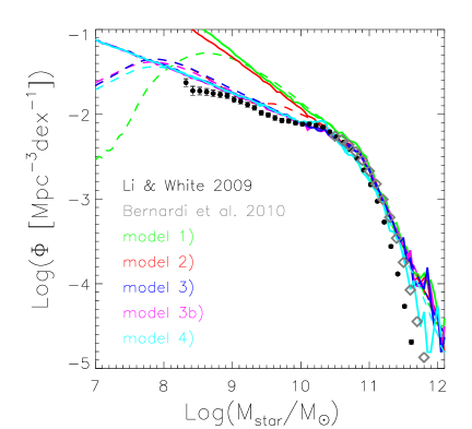
Figure 3: Stellar mass functions at $z=0$. Green, red, blue, magenta and cyan lines are for model 1), 2), 3), 3b) and 4) respectively. Solid and dashed lines are for MS-II and MS results. Black symbols with error bars are based on SDSS DR7 including both counting and cosmic variance uncertainties (Li & White, 2009; Guo et al., 2010). The grey diamonds show the functional fit to the SMF from Bernardi et al. (2010), for galaxies more massive than $10^{10.5}{\rm M}_{\odot}$.

3.2 SSFR–$M_{\rm star}$ relation

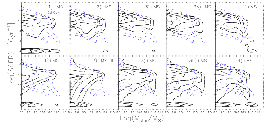
Figure 4: Contour plot of SSFR–$M_{\rm star}$ relation in different models compared with observation. Upper panels are for models applied to the MS and lower panels are for MS-II. Blue dashed contours are SDSS DR7 observation, derived from the MPA-JHU release of the SDSS DR7 catalogue, with stellar masses based on fits to the photometry following the philosophy of Kauffmann et al. (2003) and Salim et al. (2007), and SF rates based on Brinchmann et al. (2004). Black contours are the results of models 1), 2), 3), 3b) and 4). When plotting the model results, we set the minimum SSFR value to be $10^{-4}$Gyr^-1. Contours levels show regions that enclose 38, 68, 87 and 95 percent of galaxies.

The specific SF rate (SSFR) is defined as the ratio between the SF rate and the stellar mass of a galaxy. The relation between SSFR and galaxy stellar mass is a fundamental observable which needs to be reproduced by a successful model. Observationally, there is a clear trend that high mass galaxies are passively evolving with low SSFR, while low mass galaxies have high values of SSFR (Salim et al., 2007; Schiminovich et al., 2007). SAMs, however, usually predict similar, if not lower SSFR in low mass galaxies than that in massive ones (Fontanot et al., 2009). Comparisons that focus on galaxy colours also show this discrepancy, with low mass galaxies having redder colours than observed (Guo et al. 2011, but see also Weinmann et al., 2011b).

Fig. 4 shows the SSFR–$M_{\rm star}$ relation in our models, compared with SDSS observational result. The upper panels are for models applied to the MS simulation, and the lower panels show the MS-II results. In each panel, black contours are the model results, while blue contours are SDSS results. Observationally, galaxies reside in two distinct sequences in the SSFR-stellar mass plot: an active sequence with high SSFR that is more prominent for low mass galaxies, and a passive sequence with lower SSFR that contains mainly massive galaxies. The observational location of the passive sequence, however, is not well determined, due to the uncertainty on measuring the SSFR for galaxies with little SF (Salim et al., 2007). In addition, Fig. 5 shows the median SSFR as a function of galaxy stellar mass. Colored lines are predictions from our models combined with MS-II. The black solid line is the result of SDSS DR7 galaxy sample, which shows clearly that more massive galaxies have in general lower SSFR.

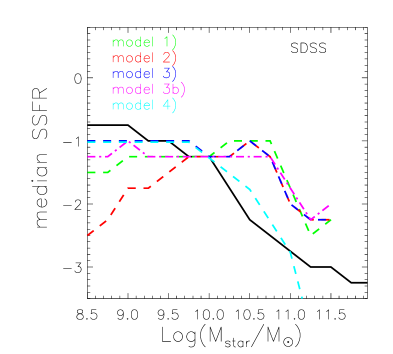
Figure 5: The median SSFR as a function of galaxy stellar mass. The black solid line shows observational results from the SDSS DR7 galaxy sample. Green, red, blue, magenta, and cyan lines are predictions from our models 1), 2), 3), 3b) and 4), combined with MS-II.

Comparing the model results applied to the MS and MS-II simulations respectively in Fig.4, it is obvious that the resolution of simulation has a large effect on the modeled SSFR for low mass galaxies, especially for models 1) and 2). This highlights the fact that resolution can have a large impact on semi-analytical model predictions (see also Guo et al. 2011). We note that the resolution dependency is weaker for models 3)-4), only affecting the passive sequence of galaxies whose location is anyway uncertain (see above). To compare the model prediction with observation for low mass galaxies, we focus on results of the models combined with the MS-II simulation. Similar to previous SAMs, model 1) predicts more passive low mass galaxies than observed, and the active sequence in model 1) is lower than observed. Its predicted median SSFR is lower than the SDSS result for galaxies less massive than $10^{9.7}{\rm M}_{\odot}$. When modifying the SF in the quiescent mode in low mass haloes in model 2), more low mass galaxies become passive, and the median SSFR is even lower than in model 1). This is due to the in general lower SF efficiency assumed in model 2) for haloes less massive than $\sim 10^{11.5}h^{-1}{\rm M}_{\odot}$, as shown in Fig. 2.

Suppressing the SF in the burst mode in low mass haloes, model 3) and 3b) predict a lower fraction of passive galaxies, with higher median SSFR for low mass galaxies. This is because the lower burst efficiency leaves galaxies with more cold gas by $z=0$. The results are then in reasonable agreement with observations. When comparing these two models in detail, model 3b) predicts on average more passive low mass galaxies and is therefore a less good match to observations. The location of the active sequence is lower than in observation, and thus not as well reproduced as in model 3).

For all models 1)-3b), the SSFR for massive galaxies are significantly overpredicted by the model. This is corrected in model 4), by modifying the cooling and SF in massive haloes. Overall, model 4) is in good agreement with the observed SSFR-$M_{\rm star}$ relation at all stellar masses.

3.3 Cold gas mass function

Fig. 6 presents the cold gas mass functions at z=0. Green, red, blue, magenta and cyan lines are for model 1), 2), 3), 3b) and 4), using the MS-II results. Crosses show the Schechter function fit to the cold gas (HI+H₂+helium) mass function given in Obreschkow & Rawlings (2009), which is derived from the HI mass function of HIPASS observation (Zwaan et al., 2005), combined with a theoretical model to describe the H₂/HI mass ratio. As pointed out in Obreschkow et al. (2009), semi-analytic models only distinguish between the hot and the cold gas phase. However, observations have revealed the existence of a significant amount of warm and ionized gas in the Milky Way (Reynolds, 2004). This motivated Obreschkow et al. (2009) to devide their model cold gas mass function by a factor of $1.45$. We follow their example here, but we stress that this factor is obviously uncertain and may well be higher, depending on galaxy mass and redshift.

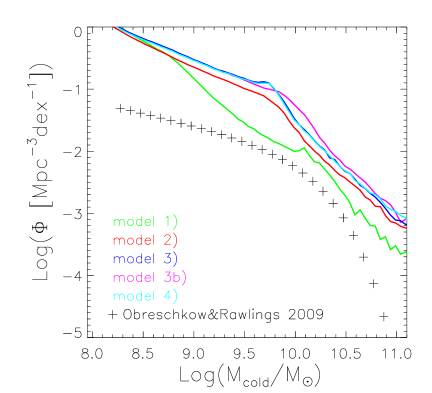
Figure 6: Cold gas mass functions at z=0. Green, red, blue, magenta and cyan lines are for model 1), 2), 3), 3b) and 4), for MS-II results. Cross symbols show the Schechter function fit for the cold gas mass function according to Obreschkow & Rawlings (2009).

The cold gas mass function of the fiducial model 1) exceeds observations. As expected, it is somewhat higher than for the DLB07 model (Obreschkow et al., 2009; Fu et al., 2010), because of the slower stripping of hot gas for satellites. The other models predict even higher amplitudes. With on average lower SF efficiencies in low mass haloes in model 2), 3) and 3b), there is much more cold gas left in the galaxies. This is not surprising, since we have left cooling and SN feedback efficiencies at the default DLB07 values. Model 4) predicts similar result of cold gas mass function as in model 3).

Although there are some uncertainties related to the determination of cold gas mass function in observation (Keres et al., 2003; Obreschkow & Rawlings, 2009; Fu et al., 2010), it seems that our models with modified SF predict drastically too much cold gas mass in galaxies. Thus, while the modifications to the SF law we suggest here improve the agreement between the statistical properties of the galaxy population in many aspects, our simple model is clearly not the final answer to all the problems that exist. This will be discussed in more detail in section 4.

3.4 Correlation function

The two point auto-correlation function of galaxies is a fundamental measure of the spatial distribution of a certain population of galaxies and is well determined by observations (e.g. Li et al., 2006). It is however not well fitted by current SAMs. For example, Guo et al. (2011) over-predict the correlation functions for low mass galaxies and on small scales. They suggest that the over-prediction of clustering of galaxies on small scales in the models can be explained by the too high value of $\sigma_{8}$ adopted by the Millennium simulation, which is $0.9$ compared to $0.81$ suggested by the WMAP-7 year result (Komatsu et al., 2011). However, it is not certain that the Guo et al. SAM combined with the correct cosmology would give correlation functions in agreement with observations (see Wang et al., 2008). Here we test the effect of modifying the SF law on the resulting correlation functions using the same underlying $N$-body simulations as Guo et al. (2011).

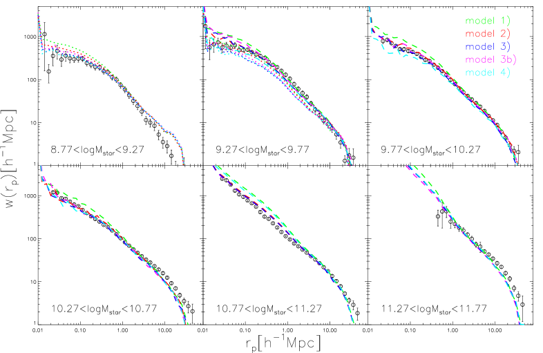
Figure 7: Projected two point auto-correlation functions of galaxies in different stellar mass bins. Circles with error bars are SDSS DR7 results (Guo et al., 2011), calculated with the same method as presented in Li et al. (2006). Green, red, blue, magenta, and cyan lines are for model 1), 2), 3), 3b), and 4) respectively. Dotted (dashed) lines are for models based on the MS-II (MS) results. For stellar mass bins with $\log(M_{\rm star})$ $>$ $9.77$, only MS results are shown. For the lowest mass bin, only MS-II results are presented.

In our models, galaxy positions are determined by the positions of haloes/subhaloes they reside in. For galaxies that have lost their host subhalo due to stripping, we use the location of the most-bound-particle of the last identified subhalo. Since we use the same dynamical friction prefactor of $\alpha_{\rm df}=5$ for models 1), 2), 3), 3b) and 4), galaxy locations in all these models are exactly the same. The only differences are in the stellar masses of galaxies that vary due to the different SF laws used. Also, the number of galaxies might be slightly different due to the effect of the stellar mass on the dynamical friction time. Consequently, the differences in the correlation functions between the models are mainly due to the different stellar mass assigned to each galaxy.

Fig. 7 shows the projected correlation functions of galaxies in different stellar mass bins, computed in the same way as in Neistein et al. (2011). Model 1) over-predicts the correlation functions for galaxies less massive than $10^{11.27}{\rm M}_{\odot}$, and at scales smaller than $\sim 1h^{-1}$Mpc. With a modified SF law in low mass haloes, correlation functions become lower at small scales for low mass galaxies, which brings model 3) into agreement with the observational results at all stellar masses. The success of model 3) in reproducing the correlation functions shows clearly that changes in the SF law, that lead to changes in the relation between stellar mass and subhalo mass, can significantly affect correlation functions. Thus, it is in general very hard to say whether a mismatch with observed correlation functions indicates a problem with baryonic recipes, or with cosmology. We thus confirm the results by Wang et al. (2008) who find that a similar match to observed correlation functions can be obtained by SAMs using different cosmological parameters, depending on the detailed baryonic recipes.

Model 3b) gives similar results to model 3) for galaxies more massive than $10^{10.27}{\rm M}_{\odot}$. For lower mass galaxies, the correlation functions of model 3b) are higher than for model 3) on small scales. Correlation functions of galaxies in model 4) are in general similar to model 3), with a somewhat worse fit in the stellar mass bin of $\log M_{\rm star}$=[10.77, 11.27].

3.5 Stellar mass functions at high $z$

At redshifts less than $\sim 0.8$, current SAMs like Monaco et al. (2007) and Somerville et al. (2008) predict SMF consistent with observations. At higher redshifts, however, models normally over-predict the abundance of galaxies less massive than $10^{10}{\rm M}_{\odot}$ (Fontanot et al., 2009; Guo et al., 2011). The same is true for the K-band luminosity function (Henriques et al., 2011). This may indicate that SF at redshifts above 0.8 is not modeled correctly in these models.

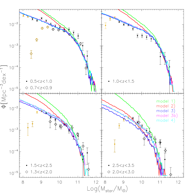
Figure 8: Stellar mass functions at redshifts above zero. Green, red, blue, magenta and cyan lines are for model 1), 2), 3), 3b) and 4). Model results combined with MS-II are shown at redshifts of $0.8,1.2,2.0,3.0$. Black points are observational results from Kajisawa et al. (2009), for all four redshift bins. In the upper left panel, observational results from Pozzetti et al. (2007) at $0.7<z<0.9$ are plotted as diamonds. Gold symbols are the data points below the completeness limit in these two observational samples. In the lower two panels, observations from Marchesini et al. (2009) for $1.3<z<2.0$ and $2.0<z<3.0$ are shown as diamonds. Observed stellar masses of galaxies are normalized to the Chabrier IMF (Chabrier, 2003).

Fig. 8 gives the results of SMF at higher redshifts in different models studied in this work. Model results are presented at redshifts of $0.8$, $1.2$, $2.0$, $3.0$, and are convolved with a Gaussian error of deviation $0.25$ dex in $\log M_{\rm star}$, to account for the various errors in estimating stellar masses in observations (Fontanot et al., 2009). Observation results are shown at comparable redshift ranges to the models. Gold symbols indicate data points below the limiting stellar mass of the observed galaxy samples, where incompleteness could be significant (Pozzetti et al., 2007; Kajisawa et al., 2009). All observational stellar masses of galaxies are normalized to the Chabrier IMF (Chabrier, 2003), to be consistent with the previously shown SDSS SMF, and the model derived SMF.

The fiducial model 1) predicts too many low mass galaxies at all redshifts. With a modified SF law in both modes, model 3) and 3b) both give consistent SMF with observations up to redshifts of around $3$. Differences of these two models can be seen at redshifts higher than $2$, where model 3b) predicts a SMF with a higher amplitude. This is because the SF efficiency in model 3b) depends on time and is higher at high redshifts.

In model 4), with the assumption that the dynamical friction time is shorter at high redshifts, SMF at redshifts of around $2-3$ are higher than in model 3), and somewhat closer to observations. The SMF in model 4) happen to be quite similar to the results of model 3b). This reflects the degeneracies inherent in SAMs, in this case between the dependence of dynamical friction time on redshift, and the dependence of SF rate on redshift.

3.6 SFR density

Fig. 9 shows the star formation rate (SFR) density as a function of redshift, as predicted by different models combined with MS simulation. Black crosses are observational results compiled by Hopkins (2007). The grey shaded region shows the 1-$\sigma$ confidence level of the observational results by Wilkins et al. (2008), which are derived indirectly from the evolution of the stellar mass function. Gold symbols are the results of Bouwens et al. (2009), including the contributions from highly dust obscured galaxies and ULIRGs. Stellar masses are normalized to the Chabrier IMF (Chabrier, 2003).

The SFR density of the fiducial model 1) shows a continuous increase with redshift and peaks at a redshift of around $3-4$, which is clearly a higher redshift than in observations. This offset is similar to the one present in the SAM of Guo et al. (2011). With a modified SF efficiency in both the quiescent and the burst mode, the SFR density of model 3) and 3b) drops dramatically at higher redshifts than $z\sim 2$. Due to the dependence of SF on Hubble time assumed in model 3b), this model gives a higher SFR density at high $z$, and a lower SFR density at low $z$ than model 3). At low redshifts, both model 3) and 3b) predict SFR density higher than the fiducial model 1), which lies slightly above the observational values.

With further suppression of cooling and SF in massive haloes in model 4), the observed sharp decline of SFR density towards low redshifts appears. Predictions of model 4) are within the observational constraints, while the SFR density peaks at redshift of around $2$. Recently, Magnelli et al. (2011) studied the evolution of dusty infrared luminosities function using Spitzer data. Assuming a constant conversion between the IR luminosity and SFR, they find that the SFR density of the Universe strongly increases towards $z=1.3$, and stays constant out to $z=2.3$. Model 4) matches the result of their observation.

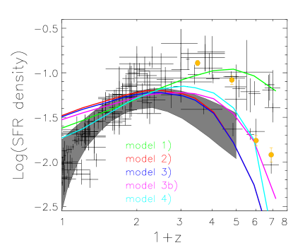
Figure 9: Cosmic star formation density as a function of redshift. Green, red, blue, magenta and cyan lines are for models 1), 2), 3), 3b) and 4) respectively, based on the MS simulation. Black crosses are observational estimates compiled by Hopkins (2007). The grey shaded region shows the 1-$\sigma$ confidence level of the observational result, as compiled by Wilkins et al. (2008). Gold symbols are the results of Bouwens et al. (2009), including the contributions from highly dust obscured galaxies and ULIRGs. Stellar masses are normalized to the Chabrier IMF (Chabrier, 2003).

4 Discussions and Conclusions

We use the method developed by Neistein & Weinmann (2010), combined with both the Millennium (MS) and Millennium-II (MS-II) cosmological simulations, to study the effect of modifying the star formation (SF) recipe in low mass galaxies. We show that by modifying SF in both the quiescent and the burst mode, the stellar mass function observed in the local Universe can be reproduced well down to $10^{8.5}{\rm M}_{\odot}$. Simultaneously, the models can fit the observed median SSFR–$M_{\rm star}$ relation for galaxies less massive than $10^{10}{\rm M}_{\odot}$, the correlation functions for galaxies more massive than $10^{8.77}{\rm M}_{\odot}$, the stellar mass functions up to redshift of around $3$, and the general trend of the SFR density as a function of redshift.

The modifications to the SF recipe in our models with respect to standard SAMs (e.g. DLB07) include:

1. no sharp threshold in the cold gas mass for SF;

2. letting the SF efficiency in the quiescent mode depend on host halo mass;

3. removing the dependence of the star formation rate on Hubble time (which came via the dependence on disk dynamical time);

4. a lower star burst efficiency in low mass haloes;

5. additional modifications of cooling and SF in massive haloes to match the properties of high mass galaxies.

Model 2) only includes the changes to the quiescent mode of SF, i) - iii). We show that this is not enough to reproduce the low mass end of the SMF, as star formation in the burst mode compensates for the changes to the SF law in the quiescent mode. This is also the reason why Lagos et al. (2010) have found that their changes to the SF law in the quiescent mode does not change the resulting SMF much. In model 3), we have thus additionally decreased SF in the burst model (modification iv), which results in a clearly improved SMF. We also considered a model 3b) which is similar to model 3), except that we allow for the usual time-dependence of the SF law (i.e. do not make modification iii). Results of model 3b) are similar to model 3) out to $z\sim 2$, except that the SSFR–$M_{\rm star}$ relation is slightly less well reproduced. It is thus not clear whether modification iii) is necessary.

Note that removing the time-dependence of the star formation efficiency is a significant change with respect to previous models. Even in the recent models of Fu et al. (2010) and Lagos et al. (2010, 2011), where SF efficiency does not depend on the disk dynamical time of galaxies, a time-dependence enters via the conversion efficiency from atomic to molecular gas, that depends on the gas density. In order to justify the behaviour we suggest in model 3), we would need to postulate a mechanism that scales with time in the opposite way than usually assumed, like for example a metallicity-dependent conversion of atomic to molecular gas (Krumholz & Dekel, 2011). We note that a weak dependence of the SF efficiency on cosmic time was seen in hydrodynamical simulations (Neistein et al., 2011b), although the reason for this behaviour is still not clear.

In our models 2) – 4), the ratio between the quiescent star formation rate and the cold gas mass, $\dot{M}_{\rm star}/M_{\rm cold}$ which is equal to the gas consumption timescale, is roughly proportional to $M_{\rm halo}^{2}$ for low mass haloes and is almost independent of halo mass for high masses. This may in fact be supported by recent observations. Recently, Shi et al. (2011) derive an extended Schimdt law from an observed galaxy sample that extends over 5 orders of magnitude in stellar density, including galaxies with low surface brightness. They find that $\dot{M}_{\rm star}/M_{\rm cold}$ is proportional to $M_{\rm star}^{0.52}$, with a 1-$\sigma$ scatter of $0.4$ dex. The stellar mass of galaxies has been claimed to obey a tight relation with the host halo mass (Conroy & Wechsler, 2009; Moster et al., 2010; Guo et al., 2010). It is proportional to $M_{\rm halo}^{2.8}$ for low mass haloes and to $M_{\rm halo}^{0.2}$ at high mass end (Wang et al., 2006). Without considering the scatter of the relation, this indicates that the observed $\dot{M}_{\rm star}/M_{\rm cold}$ is roughly proportional to $M_{\rm halo}^{1.46}$ at low masses and $M_{\rm halo}^{0.1}$ at high mass end. The dependence on halo mass in our models is therefore quite close to the observational result by Shi et al. (2011).

In all our models, the cold gas mass function of galaxies is dramatically over-predicted. This is because in DLB07, the total amount of cold gas and stellar mass exceeds the observed total amount (see Obreschkow et al., 2009; Fu et al., 2010). Decreasing SF rates in low mass galaxies while letting cooling and feedback recipes remain unchanged naturally results in an overproduction of the cold gas mass in low mass galaxies. This is not only a problem for the models we present here. As shown recently by Lu et al. (2011), when the model K-band luminosity function is forced to fit the data in the local Universe, the cold gas mass function is dramatically over-predicted in all the semi-analytic models they study. This is consistent with our models over-predicting the cold gas mass functions when we fit the stellar mass function at z=0. On the other hand, with similar cooling and supernovae feedback recipes, the models that do fit the cold gas mass function in turn have problems in reproducing the stellar mass functions (e.g. Fu et al., 2010; Obreschkow et al., 2009). In the meantime, approaches like increasing the SN feedback, that suppress the total amount of cold gas and stellar mass, lead to several other serious problems (Guo et al., 2011). These results show again that it is currently difficult for a single model to fit all observations, as mentioned in Sec. 1, unless we allow for free tuning of all recipes, including cooling (see NW2010).

Although the modifications of the SF law presented in this work help to improve the agreement with several observed statistical properties of galaxies, and seem to follow a similar scaling like the observed SF efficiencies in galaxies, the normalization of the SF efficiency cannot be correct. This is clear from the fact that our models overpredict the cold gas mass function. With a lower cold gas fraction in galaxies, the SF efficiency would obviously have to be higher than currently assumed in the models, to obtain the same SF rate.

In Fig. 10, we compare the SFR–HI mass relation in model 3) combined with MS-II (right panel), with a recent observation of the FUV derived SFR–HI mass relation for galaxies within $\sim 11$ Mpc of the Milky Way (Lee et al., 2011, left panel). The cold gas mass in model 3) is converted to the HI mass to be compared with observation, using a correction including three factors. First, as for Fig. 6, the cold gas mass from model 3) is divided by a factor of $1.45$, to account for a warm ionized gas phase, as done in Obreschkow et al. (2009). Second, we multiply the results by a factor of $0.76$ to remove the contribution of helium and heavier elements (Power et al., 2010). Finally, the hydrogen gas mass is divided by $1.4$, as adopted by Power et al. (2010) and Lu et al. (2011), to remove the contribution of $H_{2}$. Since the galaxies in the observed sample have stellar masses less than $\sim 10^{10}{\rm M}_{\odot}$, we present model results for galaxies with $8<\log(M_{\rm star})<10$. The median relation from the observations is plotted as red line in each panel. Although the observations of Lee et al. (2011) are limited to a small volume of space, the obviously different relations in observations and in model 3) indicate that the SF efficiency in model 3) is indeed much lower than in reality.

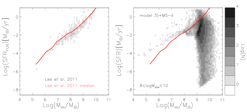
Figure 10: SF rate – HI gas relation in model 3) compared with observation. The left panel is the FUV SFR–HI mass results of Lee et al. (2011). The right panel shows results of 3) combined with MS-II simulations, for galaxies with $8<\log(M_{\rm star})<10$. Gray scales correspond to the logarithm of the number of galaxies. Red line in each panel is the median relation of the observed galaxies of Lee et al. (2011).

Fitting the most important observed properties of galaxies is not a trivial task. It is not clear up to now if this difficulty in modeling galaxy properties reflects a fundamental problem in our understanding of the dark matter universe, or if it is mainly due to an insufficient understanding of the baryonic physics involved in galaxy formation and evolution. For example, perhaps SAMs miss an important ingredient of galaxy formation, like a mechanism that preheats the gas in the universe so that it cannot cool to low mass haloes (Mo et al., 2005, but see also Crain et al. (2007)), or a form of feedback that mainly heats low entropy gas in high redshift haloes (McCarthy et al., 2011). Alternatively, it could be that cooling is over-efficient in the current SAMs for some reason.

With the tests carried out in this work, we show that only modifying star formation in the SAMs can already improve agreement with observations in several important aspects. Up to now, a high-resolution SAM that matches the SSFR-stellar mass relation at $z=0$, the SMF and its evolution, the correlation functions and the cold gas fractions of galaxies simultaneously, does not yet seem to exist. To find such a model, approaches that allow scanning of a large parameter space (Henriques et al., 2009; Lu et al., 2010; Bower et al., 2010), and approaches that allow deviations from the usually assumed functional forms for physical recipes (Neistein & Weinmann, 2010), or that include other physical processes than currently considered (Henriques & Thomas, 2010) may be promising. However, even if one or several models are found that do indeed reproduce all these fundamental observables, it will be important to identify degeneracies, and to verify whether the models are physically plausible and can be brought into agreement with alternative approaches, like predictions from hydrodynamical simulations.

Appendix A Cooling efficiencies

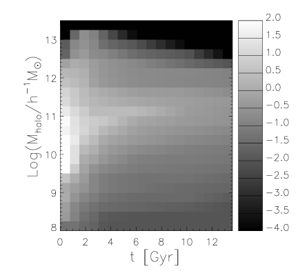
Figure 11: Cooling efficiencies as a function of halo mass and cosmic time in model 0), the fiducial model 1), and also in model 2) and 3), 3b). The gray scale shows Log values of the cooling efficiencies in units of log$[{\rm Gyr}^{-1}]$. X-axis is the cosmic time, with $13.7$ Gyr corresponding to the present day.

Our model 0) is similar to model 0 of NW2010, with a few modifications to the cooling efficiencies, which we explain below. Model 0 of NW2010 is adapted to the MS simulation, and thus only includes efficiencies down to the resolution limit of this simulation, which is $\sim 10^{10}h^{-1}{\rm M}_{\odot}$ in halo mass. To apply it to the MS-II simulation, we need efficiencies down to a lower halo mass of $\sim 10^{8}h^{-1}h^{-1}{\rm M}_{\odot}$. This is straightforward for most processes, as they are parametrized by functional forms which can easily extended to lower halo masses. The only exception are the cooling efficiencies, $f_{c}$, defined as $\Delta m_{\rm cool}=f_{c}m_{\rm hot}\Delta t$, where $\Delta m_{\rm cool}$ is the amount of gas that is cooled within a time-step $\Delta t$, and $m_{\rm hot}$ is the mass of hot gas.

In DLB07, the treatment of gas cooling follows the description of Croton et al. (2006), where cooling efficiencies are calculated according to White & Frenk (1991), assuming an isothermal gas density profile. In model 0 of NW2010, cooling efficiencies are median values computed from a large statistical sample of galaxies in DLB07, for each bin of halo mass and cosmic time. The tabulated values as a function of halo mass and time in NW2010 follow no specific functional form and can thus not easily be extended to lower mass haloes. The obvious solution would be to extract those values from the DLB07 SAM as applied to MS-II, but this is not possible for technical reasons. Therefore, we estimate cooling efficiencies for low mass haloes such that (i) the general trends of cooling efficiency as a function of halo mass and redshift are preserved, and (ii) the resulting low mass end slope and amplitude of stellar mass function at z=0 is similar to the result of DLB07 when applied to MS-II Simulation (see Fig. 1). In this way our estimates of the cooling efficiencies at a given halo mass should be similar as in the DLB07 model, when averaged over all redshifts. However, we note that the cooling efficiencies in a given redshift and halo mass bin may differ. Apart from extending the cooling efficiencies to lower mass haloes, we also apply some smoothing to the original cooling efficiencies found by NW2010, in order to smoothen the stellar mass functions.

Fig. 11 shows cooling efficiencies as a function of halo mass and cosmic time in model 0). These values are given explicitly in Table 1. The extrapolation and smoothing to the cooling efficiencies used in model 0 of NW2010 can be seen by comparing Fig. 11 with Fig. 6 in NW2010, and also comparing the values listed in Table 1 with Table 6 of NW2010. The cooling efficiencies shown in Fig. 11 and Table 1 are also applied to model 1), 2), 3) and 3b).

Fig. 12 shows the cooling efficiencies used for model 4) as presented in Sec.2.6, and table 2 lists the explicit values of those efficiencies.

Table 1: Values of cooling efficiencies in units of Gyr^-1. The values shown here are identical for models 0), 1), 2), 3) and 3b), and are plotted in Fig. 11. Halo mass is in units of $h^{-1}{\rm M}_{\odot}$ and is shown at the left column, time is in Gyr.

Log$({\rm M}_{halo})$	$t=0.80$	2.24	3.38	5.97	10.27	13.58
	$z=7$	3.0	2.0	1.0	0.3	0
8.00	-1.30	-1.60	-2.00	-2.00	-2.00	-2.00
8.25	-0.90	-1.50	-1.90	-2.00	-2.00	-2.00
8.50	-0.80	-1.30	-1.50	-1.60	-1.80	-2.00
8.75	-0.50	-1.00	-1.30	-1.50	-1.50	-1.80
9.00	-0.30	-0.80	-1.10	-1.30	-1.50	-1.60
9.25	0.10	-0.80	-1.10	-1.30	-1.30	-1.50
9.50	0.80	-0.50	-0.80	-1.10	-1.20	-1.30
9.75	1.30	-0.10	-0.50	-1.00	-1.10	-1.20
10.00	1.30	0.20	-0.30	-0.70	-1.00	-1.10
10.25	1.53	0.50	-0.07	-0.40	-0.76	-0.93
10.50	1.36	0.81	0.29	-0.23	-0.57	-0.76
10.75	1.32	0.83	0.69	-0.06	-0.38	-0.53
11.00	1.13	0.42	0.42	0.41	-0.32	-0.49
11.25	0.77	0.33	0.17	-0.06	-0.28	-0.44
11.50	0.71	0.21	0.02	-0.32	-0.41	-0.67
11.75	0.43	-0.15	-0.45	-0.71	-0.83	-0.90
12.00	0.29	-0.23	-0.51	-0.73	-0.81	-0.92
12.25	0.07	-0.28	-0.51	-0.79	-1.50	-2.00
12.50	-0.58	-0.70	-0.80	-1.50	-2.00	-4.00
12.75	-0.78	-0.70	-1.50	-2.00	-4.00	-9.00
13.00	-1.58	-0.80	-1.80	-4.00	-4.00	-9.00
13.25	-4.00	-4.00	-4.00	-9.00	-9.00	-9.00

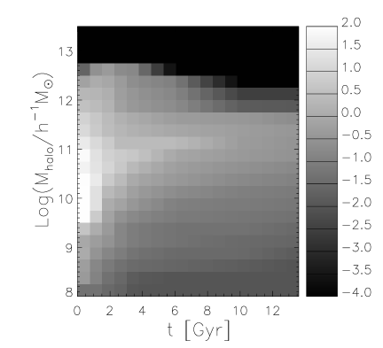
Figure 12: Cooling efficiency as a function of halo mass and cosmic time in model 4). The gray scale shows Log values of cooling efficiency in units of Log$[{\rm Gyr}^{-1}]$. X-axis is the cosmic time, with $13.7$ Gyr corresponding to present day.

Table 2: Same as table 1, but for model 4), and only showing cooling efficiencies for haloes more massive than $10^{11.5}h^{-1}{\rm M}_{\odot}$. For haloes less massive, the values are the same as in table 1.

Log$({\rm M}_{halo})$	$t=0.80$	2.24	3.38	5.97	10.27	13.58
	$z=7$	3.0	2.0	1.0	0.3	0
11.50	0.71	0.21	0.02	-0.32	-0.41	-0.67
11.75	0.43	-0.15	-0.45	-0.71	-1.83	-1.90
12.00	0.29	-0.23	-0.51	-0.83	-2.51	-2.52
12.25	0.07	-0.28	-0.70	-1.00	-4.00	-4.00
12.50	-0.58	-0.70	-0.80	-4.00	-4.00	-4.00
12.75	-9.00	-9.00	-9.00	-9.00	-9.00	-9.00
13.00	-9.00	-9.00	-9.00	-9.00	-9.00	-9.00
13.25	-9.00	-9.00	-9.00	-9.00	-9.00	-9.00

References

- Agertz et al. (2011) Agertz O., Teyssier R., Moore B., 2011, MNRAS, 410, 1391
- Avila-Reese et al. (2011) Avila-Reese V., Colín P., González-Samaniego A., Valenzuela O., Firmani C., Velázquez H., Ceverino D., 2011, ArXiv e-prints
- Baugh (2006) Baugh C. M., 2006, Reports on Progress in Physics, 69, 3101
- Baugh et al. (2005) Baugh C. M., Lacey C. G., Frenk C. S., Granato G. L., Silva L., Bressan A., Benson A. J., Cole S., 2005, MNRAS, 356, 1191
- Benson et al. (2003) Benson A. J., Bower R. G., Frenk C. S., Lacey C. G., Baugh C. M., Cole S., 2003, ApJ, 599, 38
- Bernardi et al. (2010) Bernardi M., Shankar F., Hyde J. B., Mei S., Marulli F., Sheth R. K., 2010, MNRAS, 404, 2087
- Bigiel et al. (2010) Bigiel F., Leroy A., Walter F., 2010, ArXiv e-prints
- Bigiel et al. (2008) Bigiel F., Leroy A., Walter F., Brinks E., de Blok W. J. G., Madore B., Thornley M. D., 2008, AJ, 136, 2846
- Blitz & Rosolowsky (2006) Blitz L., Rosolowsky E., 2006, ApJ, 650, 933
- Bouché et al. (2007) Bouché N., Cresci G., Davies R., Eisenhauer F., Förster Schreiber N. M., Genzel R., Gillessen S., Lehnert M., et al., 2007, ApJ, 671, 303
- Bouwens et al. (2009) Bouwens R. J., Illingworth G. D., Franx M., Chary R.-R., Meurer G. R., Conselice C. J., Ford H., Giavalisco M., van Dokkum P., 2009, ApJ, 705, 936
- Bower et al. (2006) Bower R. G., Benson A. J., Malbon R., Helly J. C., Frenk C. S., Baugh C. M., Cole S., Lacey C. G., 2006, MNRAS, 370, 645
- Bower et al. (2010) Bower R. G., Vernon I., Goldstein M., Benson A. J., Lacey C. G., Baugh C. M., Cole S., Frenk C. S., 2010, MNRAS, 407, 2017
- Boylan-Kolchin et al. (2008) Boylan-Kolchin M., Ma C.-P., Quataert E., 2008, MNRAS, 383, 93
- Boylan-Kolchin et al. (2009) Boylan-Kolchin M., Springel V., White S. D. M., Jenkins A., Lemson G., 2009, MNRAS, 398, 1150
- Brinchmann et al. (2004) Brinchmann J., Charlot S., White S. D. M., Tremonti C., Kauffmann G., Heckman T., Brinkmann J., 2004, MNRAS, 351, 1151
- Cattaneo et al. (2006) Cattaneo A., Dekel A., Devriendt J., Guiderdoni B., Blaizot J., 2006, MNRAS, 370, 1651
- Chabrier (2003) Chabrier G., 2003, PASP, 115, 763
- Cole et al. (2000) Cole S., Lacey C. G., Baugh C. M., Frenk C. S., 2000, MNRAS, 319, 168
- Colless et al. (2001) Colless M., Dalton G., Maddox S., Sutherland W., Norberg P., Cole S., Bland-Hawthorn J., Bridges T., et al., 2001, MNRAS, 328, 1039
- Conroy & Wechsler (2009) Conroy C., Wechsler R. H., 2009, ApJ, 696, 620
- Cox et al. (2004) Cox T. J., Primack J., Jonsson P., Somerville R. S., 2004, ApJ, 607, L87
- Crain et al. (2007) Crain R. A., Eke V. R., Frenk C. S., Jenkins A., McCarthy I. G., Navarro J. F., Pearce F. R., 2007, MNRAS, 377, 41
- Croton et al. (2006) Croton D. J., Springel V., White S. D. M., De Lucia G., Frenk C. S., Gao L., Jenkins A., Kauffmann G., Navarro J. F., Yoshida N., 2006, MNRAS, 365, 11
- De Lucia & Blaizot (2007) De Lucia G., Blaizot J., 2007, MNRAS, 375, 2
- Dekel et al. (2009) Dekel A., Sari R., Ceverino D., 2009, ApJ, 703, 785
- Fontanot et al. (2009) Fontanot F., De Lucia G., Monaco P., Somerville R. S., Santini P., 2009, MNRAS, 397, 1776
- Fu et al. (2010) Fu J., Guo Q., Kauffmann G., Krumholz M. R., 2010, MNRAS, 409, 515
- Genzel et al. (2010) Genzel R., Tacconi L. J., Gracia-Carpio J., Sternberg A., Cooper M. C., Shapiro K., Bolatto A., Bouché N., et al., 2010, MNRAS, 407, 2091
- Gnedin & Kravtsov (2010) Gnedin N. Y., Kravtsov A. V., 2010, ApJ, 714, 287
- Guo et al. (2011) Guo Q., White S., Boylan-Kolchin M., De Lucia G., Kauffmann G., Lemson G., Li C., Springel V., Weinmann S., 2011, MNRAS, 413, 101
- Guo et al. (2010) Guo Q., White S., Li C., Boylan-Kolchin M., 2010, MNRAS, 404, 1111
- Henriques et al. (2011) Henriques B., White S., Lemson G., Thomas P., Guo Q., Marleau G.-D., Overzier R., 2011, ArXiv e-prints
- Henriques & Thomas (2010) Henriques B. M. B., Thomas P. A., 2010, MNRAS, 403, 768
- Henriques et al. (2009) Henriques B. M. B., Thomas P. A., Oliver S., Roseboom I., 2009, MNRAS, 396, 535
- Hopkins (2007) Hopkins A. M., 2007, in J. Afonso, H. C. Ferguson, B. Mobasher, & R. Norris ed., Deepest Astronomical Surveys Vol. 380 of Astronomical Society of the Pacific Conference Series, The Star Formation History of the Universe. pp 423–+
- Hopkins et al. (2010) Hopkins P. F., Croton D., Bundy K., Khochfar S., van den Bosch F., Somerville R. S., Wetzel A., Keres D., Hernquist L., Stewart K., Younger J. D., Genel S., Ma C.-P., 2010, ApJ, 724, 915
- Jiang et al. (2008) Jiang C. Y., Jing Y. P., Faltenbacher A., Lin W. P., Li C., 2008, ApJ, 675, 1095
- Kajisawa et al. (2009) Kajisawa M., Ichikawa T., Tanaka I., Konishi M., Yamada T., Akiyama M., Suzuki R., Tokoku C., Uchimoto Y. K., Yoshikawa T., Ouchi M., Iwata I., Hamana T., Onodera M., 2009, ApJ, 702, 1393
- Kang et al. (2005) Kang X., Jing Y. P., Mo H. J., Börner G., 2005, ApJ, 631, 21
- Kauffmann (1996) Kauffmann G., 1996, MNRAS, 281, 475
- Kauffmann et al. (1999) Kauffmann G., Colberg J. M., Diaferio A., White S. D. M., 1999, MNRAS, 303, 188
- Kauffmann et al. (2003) Kauffmann G., Heckman T. M., White S. D. M., Charlot S., Tremonti C., Brinchmann J., Bruzual G., Peng E. W., et al., 2003, MNRAS, 341, 33
- Kennicutt (1989) Kennicutt Jr. R. C., 1989, ApJ, 344, 685
- Kennicutt (1998) Kennicutt Jr. R. C., 1998, ApJ, 498, 541
- Kennicutt et al. (2007) Kennicutt Jr. R. C., Calzetti D., Walter F., Helou G., Hollenbach D. J., Armus L., Bendo G., Dale D. A., et al., 2007, ApJ, 671, 333
- Keres et al. (2003) Keres D., Yun M. S., Young J. S., 2003, ApJ, 582, 659
- Khochfar & Silk (2009) Khochfar S., Silk J., 2009, ApJ, 700, L21
- Komatsu et al. (2011) Komatsu E., Smith K. M., Dunkley J., Bennett C. L., Gold B., Hinshaw G., Jarosik N., Larson D., et al., 2011, ApJS, 192, 18
- Krumholz & Dekel (2011) Krumholz M. R., Dekel A., 2011, ArXiv e-prints
- Krumholz et al. (2009) Krumholz M. R., McKee C. F., Tumlinson J., 2009, ApJ, 693, 216
- Lagos et al. (2011) Lagos C. d. P., Baugh C. M., Lacey C. G., Benson A. J., Kim H.-S., Power C., 2011, ArXiv e-prints
- Lagos et al. (2010) Lagos C. d. P., Lacey C. G., Baugh C. M., Bower R. G., Benson A. J., 2010, ArXiv e-prints
- Lee et al. (2011) Lee J. C., Gil de Paz A., Kennicutt Jr. R. C., Bothwell M., Dalcanton J., José G. Funes S. J., Johnson B. D., Sakai S., Skillman E., Tremonti C., van Zee L., 2011, ApJS, 192, 6
- Leroy et al. (2008) Leroy A. K., Walter F., Brinks E., Bigiel F., de Blok W. J. G., Madore B., Thornley M. D., 2008, AJ, 136, 2782
- Li et al. (2006) Li C., Kauffmann G., Wang L., White S. D. M., Heckman T. M., Jing Y. P., 2006, MNRAS, 373, 457
- Li & White (2009) Li C., White S. D. M., 2009, MNRAS, 398, 2177
- Lu et al. (2011) Lu Y., Mo H. J., Katz N., Weinberg M. D., 2011, ArXiv e-prints
- Lu et al. (2010) Lu Y., Mo H. J., Weinberg M. D., Katz N. S., 2010, ArXiv e-prints
- Mac Low & Ferrara (1999) Mac Low M., Ferrara A., 1999, ApJ, 513, 142
- Magnelli et al. (2011) Magnelli B., Elbaz D., Chary R. R., Dickinson M., Le Borgne D., Frayer D. T., Willmer C. N. A., 2011, ArXiv e-prints
- Marchesini et al. (2009) Marchesini D., van Dokkum P. G., Förster Schreiber N. M., Franx M., Labbé I., Wuyts S., 2009, ApJ, 701, 1765
- Martin & Kennicutt (2001) Martin C. L., Kennicutt Jr. R. C., 2001, ApJ, 555, 301
- McCarthy et al. (2011) McCarthy I. G., Schaye J., Bower R. G., Ponman T. J., Booth C. M., Dalla Vecchia C., Springel V., 2011, MNRAS, 412, 1965
- Mihos & Hernquist (1994) Mihos J. C., Hernquist L., 1994, ApJ, 425, L13
- Mihos & Hernquist (1996) Mihos J. C., Hernquist L., 1996, ApJ, 464, 641
- Mo et al. (2010) Mo H., van den Bosch F. C., White S., 2010, Galaxy Formation and Evolution
- Mo et al. (2005) Mo H. J., Yang X., van den Bosch F. C., Katz N., 2005, MNRAS, 363, 1155
- Monaco et al. (2007) Monaco P., Fontanot F., Taffoni G., 2007, MNRAS, 375, 1189
- Moster et al. (2010) Moster B. P., Somerville R. S., Maulbetsch C., van den Bosch F. C., Macciò A. V., Naab T., Oser L., 2010, ApJ, 710, 903
- Neistein et al. (2011) Neistein E., Li C., Khochfar S., Weinmann S. M., Shankar F., Boylan-Kolchin M., 2011, ArXiv e-prints
- Neistein et al. (2011b) Neistein E., Khochfar S., Dalla Vecchia C., Schaye J., 2011b, ArXiv e-prints