Pumped shot noise in adiabatically modulated graphene-based double-barrier structures

Abstract

Quantum pumping processes are accompanied by considerable quantum noise. We investigated the pumped shot noise (PSN) properties in adiabatically modulated graphene-based double-barrier structures. General expressions for adiabatically PSN in phase-coherent mesoscopic conductors are derived based on the scattering approach. It is found that comparing with the Poisson processes, the PSN is dramatically enhanced where the dc pumped current changes flow direction, which demonstrates the effect of the Klein paradox.

I Introduction

Quantum pumping is a transport mechanism which induces dc charge and spin currents in a nano-scale conductor in the absence of a bias voltage by means of a time-dependent control of some system parameters. Research on quantum pumping has attracted continued interest since its prototypical proposition due to its importance in quantum dynamic theory and potential application in various fieldsRef40 ; Ref2 ; Ref3 ; Ref4 ; Ref5 ; Ref6 ; Ref7 ; Ref8 ; Ref9 ; Ref10 ; Ref11 ; Ref12 ; Ref13 ; Ref14 ; Ref15 ; Ref16 ; Ref17 ; Ref18 ; Ref19 ; Ref20 ; Ref21 ; Ref22 ; Ref23 ; Ref24 ; Ref25 ; Ref26 ; Ref27 ; Ref28 ; Ref29 ; Ref31 ; Ref33 ; Ref36 ; Ref37 ; Ref41 ; Ref44 ; Ref45 ; Ref46 ; Ref47 . The pumped current (PC) and noise properties in various nano-scale structures were investigated such as the magnetic-barrier-modulated two dimensional electron gasRef5 , mesoscopic one-dimensional wireRef7 ; Ref23 , quantum-dot structuresRef6 ; Ref12 ; Ref13 ; Ref29 ; Ref30 ; Ref37 , mesoscopic rings with Aharonov-Casher and Aharonov-Bohm effectRef8 , magnetic tunnel junctionsRef11 , chains of tunnel-coupled metallic islandsRef26 , the nanoscale helical wireRef27 ,the Tomonaga-Luttinger liquidRef25 , and garphene-based devicesRef21 ; Ref22 ; Ref41 ; Ref44 ; Ref45 ; Ref46 ; Ref47 .

Graphene continues to attract intense interest, especially as an electronic system in which charge carriers are Dirac-like particles with linear dispersion and zero rest massRef42 . Quantum pumping properties of graphene-based devises have been investigated by several groupsRef21 ; Ref22 ; Ref41 ; Ref44 ; Ref45 ; Ref46 ; Ref47 . It is found that the direction of the PC can be reversed when a high potential barrier demonstrates stronger transparency than a low one as an effect of the Klein paradoxRef21 . The shot noise properties of a quantum pump are important in two aspects: understanding the underlying mechanisms of the shot noise may offer possible ways to improve pumping efficiency and achieve optimal pumping. On the other hand, the shot noise reflects current correlation and is sensitive to the pump source configurationRef43 . The pumped shot noise (PSN) properties may provide further information of the correlation between the transport Dirac Fermions of graphene governed by the Klein paradox and electron chirality. However, this topic has not ever been looked into. In this work, we focus on the PSN properties in adiabatically modulated graphene-based double-barrier structures based on general expressions we derived from the scattering approach. The effect of the Klein paradox on the PSN is illuminated.

II Theoretical formulation

The crystal structure of undoped graphene layers is that of a honeycomb lattice of covalent-bond carbon atoms. One valence electron corresponds to one carbon atom and the structure is composed of two sublattices, labeled by A and B. In the vicinity of the ${\bf{K}}$ point and in the presence of a potential $U$, the low-energy excitations of the gated graphene monolayer are described by the two-dimensional (2D) Dirac equation

$$v_{F}\left({{\mathbf{\sigma}}\cdot{\bf{\hat{p}}}}\right)\Psi=\left({E-U}\right)\Psi,$$ (1)

where the pseudospin matrix $\vec{\sigma}$ has components given by Pauli’s matrices and ${\bf{\hat{p}}}=(p_{x},p_{y})$ is the momentum operator. The “speed of light” of the system is $v_{F}$, i.e., the Fermi velocity ($v_{F}\approx 10^{6}$ m/s). The eigenstates of Eq. (1) are two-component spinors $\Psi=[\psi_{A},\psi_{B}]^{T}$, where $\psi_{A}$ and $\psi_{B}$ are the envelope functions associated with the probability amplitudes at the respective sublattice sites of the graphene sheet.

In the presence of a one-dimensional confining potential $U=U(x)$, we attempt solutions of Eq. (1) in the form $\psi_{A}(x,y)=\phi_{A}(x)e^{ik_{y}y}$ and $\psi_{B}(x,y)=i\phi_{B}(x)e^{ik_{y}y}$ due to the translational invariance along the $y$ direction. The resulting coupled, first-order differential equations read as

$$d\phi_{B}/d\xi+\beta\phi_{B}=(\varepsilon-u)\phi_{A},$$ (2)

$$d\phi_{A}/d\xi-\beta\phi_{A}=-(\varepsilon-u)\phi_{B}.$$ (3)

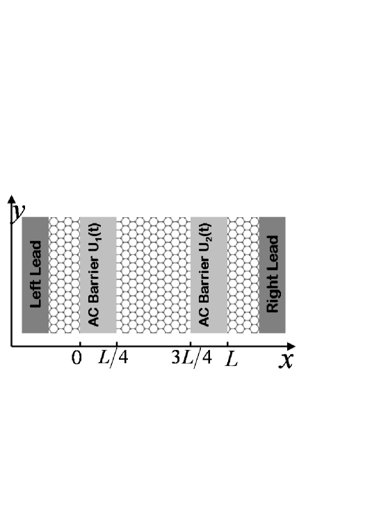
Figure 1: Sketch of the quantum pump with ac-driving-force-modulated double barriers in graphene.

Here $\xi=x/L$, $\beta=k_{y}L$, $u=UL/\hbar v_{F}$, and $\varepsilon=EL/\hbar v_{F}$ ($L$ is the width of the structure). The incident angle $\theta$ is given by $\texttt{sin}(\theta)=\beta/\varepsilon$. We consider a double-barrier structure with two square potentials of height $U_{1}$ and $U_{2}$, which can be time dependent modulated by ac gate voltages (see fig. 1). Eqs. (2) and (3) admit solutions which describe electron states confined across the well and propagating along it. As typical values $L/4$ for the barrier widths and the inter-barrier separation $L/2$ are used, the transmission and reflection amplitude $t$ and $s$ are determined by matching $\phi_{A}$ and $\phi_{B}$ at region interfaces.

Following the standard scattering approachRef3 ; Ref4 we introduce the fermionic creation and annihilation operators for the carrier scattering states. The operator $\hat{a}_{L}^{\dagger}(E,\theta,t)$ or $\hat{a}_{L}(E,\theta,t)$ creates or annihilates particles with total energy $E$ and incident angle $\theta$ in the left lead at time $t$, which are incident upon the sample. Analogously, we define the creation $\hat{b}_{L}^{\dagger}(E,\theta,t)$ and annihilation $\hat{b}_{L}(E,\theta,t)$ operators for the outgoing single-particle states. Considering a particular incident energy $E$ and incident angle $\theta$, the scattering matrix $s$ follows from the relation

$$\left({\begin{array}[]{*{20}c}{b_{L}}\\ {b_{R}}\\ \end{array}}\right)=\underbrace{\left({\begin{array}[]{*{20}c}R&{T^{\prime}}\\ T&{R^{\prime}}\\ \end{array}}\right)}_{\hat{s}}\left({\begin{array}[]{*{20}c}{a_{L}}\\ {a_{R}}\\ \end{array}}\right),$$ (4)

where, $T$ and $R$ are the scattering elements of incidence from the left reservoir and $T^{\prime}$ and $R^{\prime}$ are those from the right reservoir.

The frequency of the potential modulation is small compared to the characteristic times for traversal and reflection of electrons and the pump is thus adiabatic. In this case one can employ an instant scattering matrix approach, i.e. ${\hat{s}}(t)$ depends only parametrically on the time $t$. To realize a quantum pump one varies simultaneously two system parameters, e.g. Ref3 ; Ref4

$$\begin{array}[]{l}X_{1}\left(t\right)=X_{10}+X_{\omega,1}e^{i\left({\omega t-\varphi_{1}}\right)}+X_{\omega,1}e^{-i\left({\omega t-\varphi_{1}}\right)},\\ X_{2}\left(t\right)=X_{20}+X_{\omega,2}e^{i\left({\omega t-\varphi_{2}}\right)}+X_{\omega,2}e^{-i\left({\omega t-\varphi_{2}}\right)}.\\ \end{array}$$ (5)

Here, $X_{1}$ and $X_{2}$ are measures for the two time-dependent barrier heights $U_{1}$ and $U_{2}$ (see Fig. 1), which can be modulated by applying two low-frequency ($\omega$) alternating gate voltages. $X_{\omega,1}$ and $X_{\omega,2}$ are the corresponding oscillating amplitudes with phases $\varphi_{1/2}$; $X_{10}$ and $X_{20}$ are the static (equilibrium) components. The scattering matrix $\hat{s}$ being a function of parameters $X_{j}(t)$ depends on time.

We suppose an adiabatic quantum pump, i.e., the external parameter changes so slowly that up to corrections of order $\hbar\omega/\gamma$ ( $\gamma$ measures the escape rate), we can apply an instant scattering description using the scattering matrix ${\hat{s}}\left(t\right)$ frozen at some time $t$. Usually the varying of the wave is sufficiently smooth on the scale of the dwell time. And we assume that the amplitude ${X_{\omega,j}}$ is small enough to keep only the terms linear in ${X_{\omega,j}}$ in an expansion of the scattering matrixRef4

$$\hat{s}\left(t\right)\approx\hat{s}^{0}+\hat{s}^{-\omega}e^{i\omega t}+\hat{s}^{+\omega}e^{-i\omega t}.$$ (6)

In the limit of small frequencies the amplitudes $\hat{s}^{\pm\omega}$ can be expressed in terms of parametric derivatives of the on-shell scattering matrix $\hat{s}$,

$$\hat{s}^{\pm\omega}=\sum\limits_{j}{X_{\omega,j}e^{\pm i\varphi_{j}}\frac{{\partial\hat{s}}}{{\partial X_{j}}}}.$$ (7)

The expansion, Eq. (6), is equivalent to the nearest sideband approximation which implies that a scattered electron can absorb or emit only one energy quantum $\hbar\omega$ before it leaves the scattering region.

The problem of current noise in a quantum pump is closely connected with the problem of quantization of the charge pumped in one cycle. On the other hand, the noise in mesoscopic phase-coherent conductors is interesting in itself because it is very sensitive to quantum mechanical interference effects and can give additional information about the scattering matrixRef4 . To describe the current-current fluctuations we will use the correlation functionRef48

$$S_{\alpha\beta}\left({t,t^{\prime}}\right)=\frac{1}{2}\left\langle{\Delta\hat{I}_{\alpha}\left(t\right)\Delta\hat{I}_{\beta}\left({t^{\prime}}\right)+\Delta\hat{I}_{\beta}\left({t^{\prime}}\right)\Delta\hat{I}_{\alpha}\left(t\right)}\right\rangle,$$ (8)

with $\Delta\hat{I}=\hat{I}-\left\langle{\hat{I}}\right\rangle$ and $\hat{I}_{\alpha}\left(t\right)$ is the quantum-mechanical current operator in the lead $\alpha$ as

$$\hat{I}_{\alpha}\left(t\right)=\frac{e}{h}\left[{\hat{b}_{\alpha}^{\dagger}\left(t\right)\hat{b}_{\alpha}\left(t\right)-\hat{a}_{\alpha}^{\dagger}\left(t\right)\hat{a}_{\alpha}\left(t\right)}\right].$$ (9)

The time-dependent operator is $\hat{a}_{\alpha}\left(t\right)=\int{dE\hat{a}_{\alpha}\left(E\right)e^{{{-iEt}\mathord{\left/{\vphantom{{-iEt}\hbar}}\right.\kern-1.2pt}\hbar}}}$ and $\hat{b}_{\alpha}\left(t\right)=\sum\limits_{\beta}{s_{\alpha\beta}\left(t\right)\hat{a}_{\beta}\left(t\right)}$ with ${s_{\alpha\beta}}$ an element of the instant scattering matrix $\hat{s}$. Note that in the case of a time-dependent scatterer the correlation function depends on two times $t$ and $t^{\prime}$. Here we are interested in the noise averaged over a long time ($\Delta t\gg{{2\pi}\mathord{\left/{\vphantom{{2\pi}\omega}}\right.\kern-1.2pt}\omega}$) and we investigate

$$S_{\alpha\beta}\left(t\right)=\frac{\omega}{{2\pi}}\int_{0}^{{{2\pi}\mathord{\left/{\vphantom{{2\pi}\omega}}\right.\kern-1.2pt}\omega}}{dtS_{\alpha\beta}\left({t,t^{\prime}}\right)}.$$ (10)

In addition we restrict our consideration to the zero-frequency component of the noise spectra $S_{\alpha\beta}=\int{dtS_{\alpha\beta}\left(t\right)}$. Substituting the current operator Eq. (9), and taking into account Eqs. (4) and (6) we can write the time-averaged zero-frequency PSN as

$$\begin{array}[]{c}S_{\alpha\beta}=\frac{{e^{2}\omega}}{{2\pi}}\sum\limits_{\mu\nu j_{1}j_{2}}{X_{\omega,j_{2}}X_{\omega,j_{1}}s_{\upsilon\beta}^{{\dagger}0}\frac{{\partial s_{\alpha\nu}}}{{\partial X_{j_{1}}}}\frac{{\partial s_{\beta\mu}}}{{\partial X_{j_{2}}}}s_{\mu\alpha}^{{\dagger}0}\cos\left({\varphi_{j_{1}}-\varphi_{j_{2}}}\right)}\\ \hskip 22.76228pt+\frac{{e^{2}\omega}}{{2\pi}}\sum\limits_{\mu\nu j_{1}j_{2}}{X_{\omega,j_{2}}X_{\omega,j_{1}}s_{\upsilon\beta}^{{\dagger}0}s_{\alpha\nu}^{0}\frac{{\partial s_{\beta\mu}}}{{\partial X_{j_{2}}}}\frac{{\partial s_{\mu\alpha}^{\dagger}}}{{\partial X_{j_{1}}}}\cos\left({\varphi_{j_{1}}-\varphi_{j_{2}}}\right)}\\ \hskip 22.76228pt+\frac{{e^{2}\omega}}{{2\pi}}\sum\limits_{\mu\nu j_{1}j_{2}}{X_{\omega,j_{2}}X_{\omega,j_{1}}\frac{{\partial s_{\upsilon\beta}^{\dagger}}}{{\partial X_{j_{2}}}}\frac{{\partial s_{\alpha\upsilon}}}{{\partial X_{j_{1}}}}s_{\beta\mu}^{0}s_{\mu\alpha}^{{\dagger}0}\cos\left({\varphi_{j_{1}}-\varphi_{j_{2}}}\right)}\\ \hskip 22.76228pt+\frac{{e^{2}\omega}}{{2\pi}}\sum\limits_{\mu\nu j_{1}j_{2}}{X_{\omega,j_{2}}X_{\omega,j_{1}}\frac{{\partial s_{\upsilon\beta}^{\dagger}}}{{\partial X_{j_{2}}}}s_{\alpha\upsilon}^{0}s_{\beta\mu}^{0}\frac{{\partial s_{\mu\alpha}^{\dagger}}}{{\partial X_{j_{1}}}}\cos\left({\varphi_{j_{1}}-\varphi_{j_{2}}}\right)}\\ +\frac{{e^{2}\omega}}{{2\pi}}\sum\limits_{\mu\upsilon j_{1}j_{2}j_{3}j_{4}}{\left[{X_{\omega,j_{1}}X_{\omega,j_{4}}X_{\omega,j_{2}}X_{\omega,j_{3}}\frac{{\partial s_{\beta\mu}}}{{\partial X_{j_{4}}}}\frac{{\partial s_{\mu\alpha}^{\dagger}}}{{\partial X_{j_{1}}}}}\right.}\\ \hskip 22.76228pt\left.{\times\frac{{\partial s_{\alpha\upsilon}}}{{\partial X_{j_{2}}}}\frac{{\partial s_{\upsilon\beta}^{\dagger}}}{{\partial X_{j_{3}}}}\cos\left({\varphi_{j_{4}}-\varphi_{j_{1}}+\varphi_{j_{3}}-\varphi_{j_{2}}}\right)}\right].\\ \end{array}$$ (11)

Eq. (11) is the central result of this manuscript, which can be used to investigate the time-averaged zero-frequency PSN properties in different nanoscale adiabatic pumping structures. Detailed derivation is provided in the Appendix A.

The PC could be expressed in terms of the scattering matrix as followsRef4 ; Ref21 .

$$I_{\alpha}=\frac{{e\omega}}{{2\pi}}\sum\limits_{\beta j_{1}j_{2}}{X_{\omega,j_{1}}X_{\omega,j_{2}}\frac{{\partial s_{\alpha\beta}}}{{\partial X_{j_{1}}}}\frac{{\partial s_{\alpha\beta}^{*}}}{{\partial X_{j_{2}}}}2i\sin\left({\varphi_{j_{1}}-\varphi_{j_{2}}}\right)}.$$ (12)

Due to current conservation, it can be seen that for a two-lead (left and right) quantum pump (see Fig. 1), $I_{L}=I_{R}$ and $S_{LL}=S_{RR}=-S_{LR}=-S_{RL}$. It is reasonable to consider only the $I_{L}$ and $S_{LL}$. The symbols $I_{p}$ and $S_{p}$ are used for the PC $I_{L}$ and PSN $S_{LL}$, respectively. A convenient measure for the relative noise strength is the Fano factor defined by $F_{p}=S_{p}/2eI_{p}$, which characterizes the noise with respect to the Poisson processes. The Poissonian shot noise in the configuration of a quantum pump is discussed in the Appendix B.

III Numerical results and interpretations

We consider the PSN properties in the graphene-based conductor modulated by two ac gate voltages sketched in Fig. 1. In numerical calculations, the parameters $U_{10}=U_{20}=100$ meV, $L=200$ nm, $U_{1\omega}=U_{2\omega}=0.01$ meV. The phase difference of the two oscillating gate potentials $\phi=\varphi_{2}-\varphi_{1}$ in the radian unit.

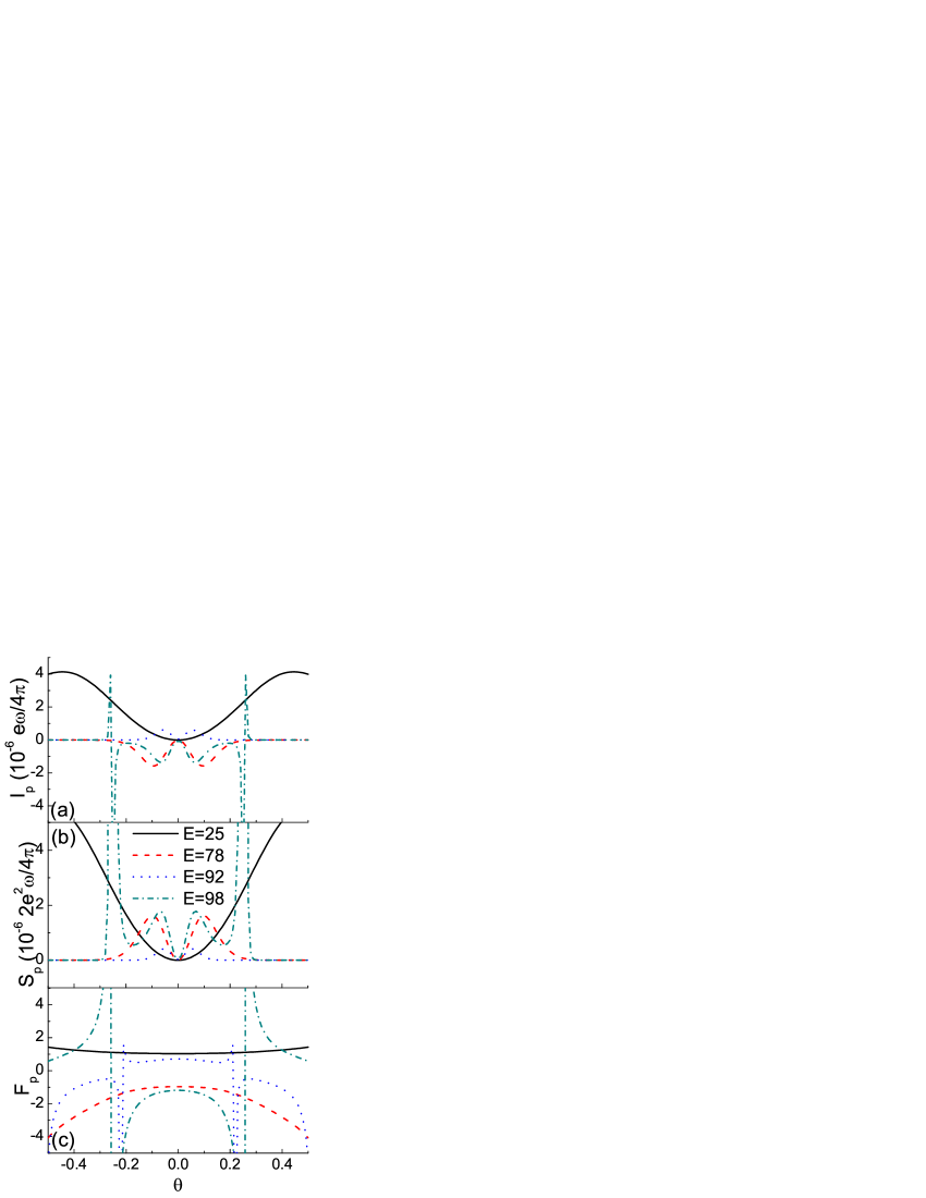
Figure 2: Pumped current (a), shot noise (b), Fano factor (c) as functions of the incident angle for different Fermi energies. Driving amplitude $U_{\omega 1}=U_{\omega 2}=0.01$ meV. Driving phase $\varphi_{1}=0.1$ and $\varphi_{2}=0.6$. The Fermi energy is measured in meV.

The PC, PSN, and Fano factor as functions of the incident angle $\theta$ for different Fermi energies are shown in Fig. 2. Electrons at the Fermi levels of the reservoirs are driven to flow in one direction by modulating the two barriers with a phase lag, which results in a dc PC at zero bias. The direction of the PC can be reversed when a high potential barrier demonstrates stronger transparency than a low one, which results from the Klein paradoxRef21 . The PSN is nonnegative as it measures the PC-PC correlation flowing in the same direction. It can be seen that the PSN increases when the PC is increased. The Poisson shot noise demonstrates the process governed by uncorrelated electrons and barrier gates without conduction structure (see the Apendix B). In graphene conductors, quantum states below potential barriers are hole states. Transmission from electron states outside the potential barriers into the hole states inside the potential barriers is characterized by the Klein paradox. For some incident angles and certain potential heights when chirality meets, the potential barrier is transparent. For other situations violating chirality alignment, the potential barrier is opaque. As the ac drivers modulate the potential barriers in time, the transmission is varied and a dc current is pumped from one reservoir to the other. Klein paradox virtually correlates the hole states with the electron states. Therefore, the PSN is remarkably enhanced beyond the Poisson value, the latter of which indicates uncorrelated transport. The PSN relative to the Poisson value measured by the Fano factor is presented in Fig. 2 (c). It can be seen that the Fano factor is above 1. Klein paradox induced virtual correlation between electrons and holes enhances the PSN beyond the Poisson value. It is also revealed in Fig. 2 that the PSN and Fano factor are extremely large at the incident angle when the PC reverses direction. At those incident angles, the chirality alignment is reversed, which induces extraordinary correlation between electrons and holes in virtual transport processes.

The PC, PSN, and Fano factor as functions of the Fermi energy of the two reservoirs $E$ for the incident angle $\theta=0.01$ are shown in Fig. 3. The absolute value of the PC is in maximums at transmission peaks of the two-barrier graphene structure. Around the transmission peaks, the PC reverses direction. In our pumping configuration, ${\varphi_{1}}<{\varphi_{2}}$. The right gate opens in advance of the left gate. In quantum pumps constructed by other conductors, the PC always flows from the right to the left reservoir at the ${\varphi_{1}}<{\varphi_{2}}$ phase lag. As a result of the Klein paradox, higher potential barrier demonstrates stronger transmission when the chirality alignment meets and the PC reverses direction. The chirality consistency favoring transmission is different between the incident energy above and below the peak energy. When the Fermi energy is smaller than the Dirac point 100 meV, above the peak energy, higher potential barrier demonstrates stronger transmission and the PC flows from the left reservoir to the right. Below the peak energy, higher potential barrier demonstrates weaker transmission and the PC flows from the right reservoir to the left. When the Fermi energy is larger than the Dirac point, the PC direction is reversed as the transmission configuration is reversed. Larger PCs have relatively stronger current-current correlation. The shot noise demonstrates peaks at the PC peaks as shown in Fig. 3 (b). The shot noise is positive since the rightward current flow correlates with the rightward current flow and vice versa. The Fano factor is above 1 due to the Klein paradox induced virtual correlation between electrons and holes. At energies when the PC reverses direction, the shot noise is extraordinarily enhanced beyond the Poisson value. At those energies, the chirality alignment is reversed, which induces extraordinary correlation between electrons and holes in virtual transport processes.

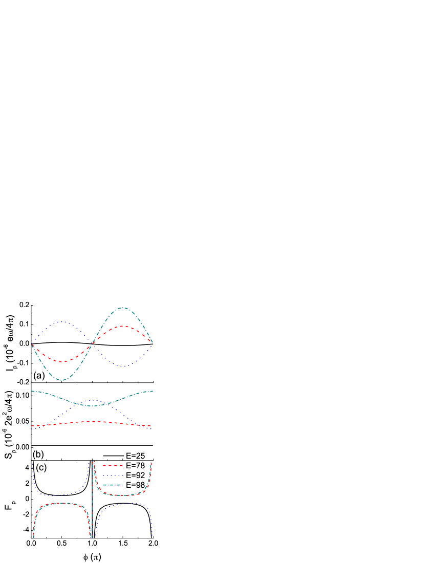
Figure 4: Pumped current (a), shot noise (b), Fano factor (c) as functions of the driving phase difference for different Fermi energies. Driving amplitude $U_{\omega 1}=U_{\omega 2}=0.01$ meV. Incident angle $\theta=0.01$. The Fermi energy is measured in meV.

The PC, PSN, and the Fano factor as functions of the driving phase difference are shown in Fig. 4. The PC varies with the driving phase $\phi$ in sinusoidal function and the PSN in cosinusoidal function, which can be already seen in Eqs. (11) and (12). The last term of Eq. (11) is a product of four pumping amplitudes, four derivatives of the scattering-matrix elements relative to the oscillating parameter, and a $\cos 2\phi$ function. As small pumping amplitudes are considered in our approach, the magnitude of this term is negligible. Therefore, the PSN is a function of $\cos\phi$ and no $\cos 2\phi$-form modulation is observable. From Fig. 4 (c) we can see that for all the Fermi energies considered the Fano factor varies with $\phi$ in similar forms. When the Fermi energy $E$ and the incident angle $\theta$ are fixed, the transmission features of the conducting structure are fixed. The variation of the pumping phase lag would not change the transmission features. For all Fermi energies and incident angles, the pumping properties as functions of the driving phase difference are similar. For configurations of $E$ and $\theta$ that higher potential barriers have stronger transmission, the PC and Fano factor are positive at ${\varphi_{2}}-{\varphi_{1}}\in\left[{\pi,2\pi}\right]$ and negative at ${\varphi_{2}}-{\varphi_{1}}\in\left[{0,\pi}\right]$. And for configurations of $E$ and $\theta$ that lower potential barriers have stronger transmission, the sign of the PC and Fano factor is reversed. At the phase lag $0$, $\pi$ , and $2\pi$, the PC changes direction as a result of the swap of the opening order of the two gates. When the PC changes direction, interaction of electrons and holes in virtual processes is enhanced and the Fano factor demonstrates a sharp rise.

IV Conclusions

In summary, the PSN properties in adiabatically modulated graphene-based double-barrier structures are investigated. Within the scattering-matrix framework, general expressions for adiabatically PSN in phase-coherent mesoscopic conductors are derived. In comparison with uncorrelated Poisson processes, numerical results of the PC, PSN, and Fano factor as functions of the incident angle, the Fermi energy of the reservoirs, and the phase difference of the two oscillating parameters are presented. It is revealed that the PSN is greatly enhanced beyond the Poisson process due to interactions of electrons and holes in Klein-type virtual tunneling processes. In particular, the PSN is dramatically enhanced at the energy and incident angle configuration with which the dc pumped current changes flow direction.

V Acknowledgements

This project was supported by the National Natural Science Foundation of China (No. 11004063), the Fundamental Research Funds for the Central Universities, SCUT (No. 2009ZM0299), the Nature Science Foundation of SCUT (No. x2lxE5090410) and the Graduate Course Construction Project of SCUT (No. yjzk2009001 and No. yjzk2010009).

VI Appendix A: Derivation of the pumped shot noise

To describe the current-current fluctuations we will use the correlation functionRef48

$$\begin{array}[]{l}S_{\alpha\beta}\left({t,t^{\prime}}\right)=\frac{1}{2}\left\langle{\Delta\hat{I}_{\alpha}\left(t\right)\Delta\hat{I}_{\beta}\left({t^{\prime}}\right)+\Delta\hat{I}_{\beta}\left({t^{\prime}}\right)\Delta\hat{I}_{\alpha}\left(t\right)}\right\rangle\\ \hskip 48.36958pt=\frac{1}{2}\left[{\left\langle{\hat{I}_{\alpha}\left(t\right)\hat{I}_{\beta}\left({t^{\prime}}\right)}\right\rangle+\left\langle{\hat{I}_{\beta}\left({t^{\prime}}\right)\hat{I}_{\alpha}\left(t\right)}\right\rangle}\right.\\ \hskip 48.36958pt\left.{-\left\langle{\hat{I}_{\alpha}\left(t\right)}\right\rangle\left\langle{\hat{I}_{\beta}\left({t^{\prime}}\right)}\right\rangle-\left\langle{\hat{I}_{\beta}\left({t^{\prime}}\right)}\right\rangle\left\langle{\hat{I}_{\alpha}\left(t\right)}\right\rangle}\right],\\ \end{array}$$ (13)

with $\Delta\hat{I}=\hat{I}-\left\langle{\hat{I}}\right\rangle$ and $\hat{I}_{\alpha}\left(t\right)$ is the quantum-mechanical current operator in the lead $\alpha$. The zero-frequency pumped shot noise (PSN) averaged over a long time ($\Delta t\gg{{2\pi}\mathord{\left/{\vphantom{{2\pi}\omega}}\right.\kern-1.2pt}\omega}$) is the time integral of $S_{\alpha\beta}\left({t,t^{\prime}}\right)$ as follows.

$$S_{\alpha\beta}=\frac{\omega}{{2\pi}}\int_{-\infty}^{+\infty}{\int_{0}^{\frac{{2\pi}}{\omega}}{S_{\alpha\beta}\left({t,t^{\prime}}\right)dt^{\prime}dt}}$$ (14)

The first term in the PSN is

$$\frac{1}{2}\frac{\omega}{{2\pi}}\int_{-\infty}^{+\infty}{\int_{0}^{\frac{{2\pi}}{\omega}}{\left\langle{\hat{I}_{\alpha}\left(t\right)\hat{I}_{\beta}\left({t^{\prime}}\right)}\right\rangle dt^{\prime}dt}}$$ (15)

with

$$\hat{I}_{\alpha}\left(t\right)=\frac{e}{h}\left[{\hat{b}_{\alpha}^{\dagger}\left(t\right)\hat{b}_{\alpha}\left(t\right)-\hat{a}_{\alpha}^{\dagger}\left(t\right)\hat{a}_{\alpha}\left(t\right)}\right],$$ (16)

and

$$\hat{I}_{\beta}\left({t^{\prime}}\right)=\frac{e}{h}\left[{\hat{b}_{\beta}^{\dagger}\left({t^{\prime}}\right)\hat{b}_{\beta}\left({t^{\prime}}\right)-\hat{a}_{\beta}^{\dagger}\left({t^{\prime}}\right)\hat{a}_{\beta}\left({t^{\prime}}\right)}\right].$$ (17)

Therefore, we have

$$\begin{array}[]{c}\hat{I}_{\alpha}\left(t\right)\hat{I}_{\beta}\left({t^{\prime}}\right)=\frac{{e^{2}}}{{h^{2}}}\left[{\hat{b}_{\alpha}^{\dagger}\left(t\right)\hat{b}_{\alpha}\left(t\right)\hat{b}_{\beta}^{\dagger}\left({t^{\prime}}\right)\hat{b}_{\beta}\left({t^{\prime}}\right)}\right.\\ \hskip 34.14322pt-\hat{b}_{\alpha}^{\dagger}\left(t\right)\hat{b}_{\alpha}\left(t\right)\hat{a}_{\beta}^{\dagger}\left({t^{\prime}}\right)\hat{a}_{\beta}\left({t^{\prime}}\right)\\ \hskip 34.14322pt-\hat{a}_{\alpha}^{\dagger}\left(t\right)\hat{a}_{\alpha}\left(t\right)\hat{b}_{\beta}^{\dagger}\left({t^{\prime}}\right)\hat{b}_{\beta}\left({t^{\prime}}\right)\\ \hskip 45.52458pt\left.{+\hat{a}_{\alpha}^{\dagger}\left(t\right)\hat{a}_{\alpha}\left(t\right)\hat{a}_{\beta}^{\dagger}\left({t^{\prime}}\right)\hat{a}_{\beta}\left({t^{\prime}}\right)}\right].\\ \end{array}$$ (18)

Substituting $\hat{b}_{\alpha}\left(t\right)=\sum\limits_{\beta}{s_{\alpha\beta}\left(t\right)\hat{a}_{\beta}\left(t\right)}$ into the above equation, we have

$$\begin{array}[]{c}\hat{I}_{\alpha}\left(t\right)\hat{I}_{\beta}\left({t^{\prime}}\right)=\frac{{e^{2}}}{{h^{2}}}\sum\limits_{\mu\upsilon\xi\eta}{\hat{a}_{\mu}^{\dagger}\left(t\right)s_{\mu\alpha}^{\dagger}\left(t\right)s_{\alpha\upsilon}\left(t\right)\hat{a}_{\upsilon}\left(t\right)\hat{a}_{\xi}^{\dagger}\left({t^{\prime}}\right)s_{\xi\beta}^{\dagger}\left({t^{\prime}}\right)s_{\beta\eta}\left({t^{\prime}}\right)\hat{a}_{\eta}\left({t^{\prime}}\right)}\\ -\frac{{e^{2}}}{{h^{2}}}\sum\limits_{\mu\upsilon}{\hat{a}_{\mu}^{\dagger}\left(t\right)s_{\mu\alpha}^{\dagger}\left(t\right)s_{\alpha\upsilon}\left(t\right)\hat{a}_{\upsilon}\left(t\right)\hat{a}_{\beta}^{\dagger}\left({t^{\prime}}\right)\hat{a}_{\beta}\left({t^{\prime}}\right)}\\ -\frac{{e^{2}}}{{h^{2}}}\sum\limits_{\mu\upsilon}{\hat{a}_{\alpha}^{\dagger}\left(t\right)\hat{a}_{\alpha}\left(t\right)\hat{a}_{\mu}^{\dagger}\left({t^{\prime}}\right)s_{\mu\beta}^{\dagger}\left({t^{\prime}}\right)s_{\beta\upsilon}\left({t^{\prime}}\right)\hat{a}_{\upsilon}\left({t^{\prime}}\right)}\\ +\frac{{e^{2}}}{{h^{2}}}\hat{a}_{\alpha}^{\dagger}\left(t\right)\hat{a}_{\alpha}\left(t\right)\hat{a}_{\beta}^{\dagger}\left({t^{\prime}}\right)\hat{a}_{\beta}\left({t^{\prime}}\right),\\ \end{array}$$ (19)

and

$$\begin{array}[]{c}\left\langle{\hat{I}_{\alpha}\left(t\right)}\right\rangle\left\langle{\hat{I}_{\beta}\left({t^{\prime}}\right)}\right\rangle=\frac{{e^{2}}}{{h^{2}}}\sum\limits_{\mu\upsilon\xi\eta}{\left\langle{\hat{a}_{\mu}^{\dagger}\left(t\right)s_{\mu\alpha}^{\dagger}\left(t\right)s_{\alpha\upsilon}\left(t\right)\hat{a}_{\upsilon}\left(t\right)}\right\rangle\left\langle{\hat{a}_{\xi}^{\dagger}\left({t^{\prime}}\right)s_{\xi\beta}^{\dagger}\left({t^{\prime}}\right)s_{\beta\eta}\left({t^{\prime}}\right)\hat{a}_{\eta}\left({t^{\prime}}\right)}\right\rangle}\\ \hskip 14.22636pt-\frac{{e^{2}}}{{h^{2}}}\sum\limits_{\mu\upsilon}{\left\langle{\hat{a}_{\mu}^{\dagger}\left(t\right)s_{\mu\alpha}^{\dagger}\left(t\right)s_{\alpha\upsilon}\left(t\right)\hat{a}_{\upsilon}\left(t\right)}\right\rangle\left\langle{\hat{a}_{\beta}^{\dagger}\left({t^{\prime}}\right)\hat{a}_{\beta}\left({t^{\prime}}\right)}\right\rangle}\\ \hskip 19.91684pt-\frac{{e^{2}}}{{h^{2}}}\sum\limits_{\mu\upsilon}{\left\langle{\hat{a}_{\alpha}^{\dagger}\left(t\right)\hat{a}_{\alpha}\left(t\right)}\right\rangle\left\langle{\hat{a}_{\mu}^{\dagger}\left({t^{\prime}}\right)s_{\mu\beta}^{\dagger}\left({t^{\prime}}\right)s_{\beta\upsilon}\left({t^{\prime}}\right)\hat{a}_{\upsilon}\left({t^{\prime}}\right)}\right\rangle}\\ +\frac{{e^{2}}}{{h^{2}}}\left\langle{\hat{a}_{\alpha}^{\dagger}\left(t\right)\hat{a}_{\alpha}\left(t\right)}\right\rangle\left\langle{\hat{a}_{\beta}^{\dagger}\left({t^{\prime}}\right)\hat{a}_{\beta}\left({t^{\prime}}\right)}\right\rangle.\\ \end{array}$$ (20)

Using $\hat{a}_{\alpha}\left(t\right)=\int{dE\hat{a}_{\alpha}\left(E\right)e^{{{-iEt}\mathord{\left/{\vphantom{{-iEt}\hbar}}\right.\kern-1.2pt}\hbar}}}$ and $\hat{a}_{\alpha}^{{\dagger}}\left(t\right)=\int{dE\hat{a}_{\alpha}^{{\dagger}}\left(E\right)e^{{{iEt}\mathord{\left/{\vphantom{{-iEt}\hbar}}\right.\kern-1.2pt}\hbar}}}$, the first term in Eq. (19) reads

$$\begin{array}[]{l}\frac{{e^{2}}}{{h^{2}}}\sum\limits_{\mu\upsilon\xi\eta}{\int{dE_{1}dE_{2}dE_{3}dE_{4}}\hat{a}_{\mu}^{\dagger}\left({E_{1}}\right)e^{{{iE_{1}t}\mathord{\left/{\vphantom{{iE_{1}t}\hbar}}\right.\kern-1.2pt}\hbar}}s_{\mu\alpha}^{\dagger}\left(t\right)s_{\alpha\upsilon}\left(t\right)\hat{a}_{\upsilon}\left({E_{2}}\right)e^{{{-iE_{2}t}\mathord{\left/{\vphantom{{-iE_{2}t}\hbar}}\right.\kern-1.2pt}\hbar}}}\\ \hskip 17.07182pt\times\hat{a}_{\xi}^{\dagger}\left({E_{3}}\right)e^{{{iE_{3}t^{\prime}}\mathord{\left/{\vphantom{{iE_{3}t^{\prime}}\hbar}}\right.\kern-1.2pt}\hbar}}s_{\xi\beta}^{\dagger}\left({t^{\prime}}\right)s_{\beta\eta}\left({t^{\prime}}\right)\hat{a}_{\eta}\left({E_{4}}\right)e^{{{-iE_{4}t^{\prime}}\mathord{\left/{\vphantom{{-iE_{4}t^{\prime}}\hbar}}\right.\kern-1.2pt}\hbar}}.\\ \end{array}$$ (21)

Wick’s theorem gives the quantum statistical expectation value of products of four operators $\hat{a}$. For a Fermi gas at equilibrium this expectation value isRef48

$$\begin{array}[]{l}\left\langle{\hat{a}_{\mu}^{\dagger}\left({E_{1}}\right)\hat{a}_{\upsilon}\left({E_{2}}\right)\hat{a}_{\xi}^{\dagger}\left({E_{3}}\right)\hat{a}_{\eta}\left({E_{4}}\right)}\right\rangle-\left\langle{\hat{a}_{\mu}^{\dagger}\left({E_{1}}\right)\hat{a}_{\upsilon}\left({E_{2}}\right)}\right\rangle\left\langle{\hat{a}_{\xi}^{\dagger}\left({E_{3}}\right)\hat{a}_{\eta}\left({E_{4}}\right)}\right\rangle\\ =\delta_{\mu\eta}\delta_{\upsilon\xi}\delta\left({E_{1}-E_{4}}\right)\delta\left({E_{2}-E_{3}}\right)f_{\mu}\left({E_{1}}\right)\left[{1-f_{\upsilon}\left({E_{2}}\right)}\right].\\ \end{array}$$ (22)

$f_{\alpha}(E)$ is the Fermi distribution function of the $\alpha$ reservoir connected to the adiabatically modulated conductor. Substituting Eq. (22) into the first term of $\left\langle{\hat{I}_{\alpha}\left(t\right)\hat{I}_{\beta}\left({t^{\prime}}\right)}\right\rangle-\left\langle{\hat{I}_{\alpha}\left(t\right)}\right\rangle\left\langle{\hat{I}_{\beta}\left({t^{\prime}}\right)}\right\rangle$, we have

$$\begin{array}[]{l}\frac{{e^{2}}}{{h^{2}}}\sum\limits_{\mu\upsilon\xi\eta}{\int{dE_{1}dE_{2}dE_{3}dE_{4}}\delta_{\mu\eta}\delta_{\nu\xi}\delta\left({E_{1}-E_{4}}\right)\delta\left({E_{2}-E_{3}}\right)f_{\mu}\left({E_{1}}\right)\left[{1-f_{\nu}\left({E_{2}}\right)}\right]}\\ \hskip 17.07182pt\times e^{{{iE_{1}t}\mathord{\left/{\vphantom{{iE_{1}t}\hbar}}\right.\kern-1.2pt}\hbar}}s_{\mu\alpha}^{\dagger}\left(t\right)s_{\alpha\upsilon}\left(t\right)e^{{{-iE_{2}t}\mathord{\left/{\vphantom{{-iE_{2}t}\hbar}}\right.\kern-1.2pt}\hbar}}e^{{{iE_{3}t^{\prime}}\mathord{\left/{\vphantom{{iE_{3}t^{\prime}}\hbar}}\right.\kern-1.2pt}\hbar}}s_{\xi\beta}^{\dagger}\left({t^{\prime}}\right)s_{\beta\eta}\left({t^{\prime}}\right)e^{{{-iE_{4}t^{\prime}}\mathord{\left/{\vphantom{{-iE_{4}t^{\prime}}\hbar}}\right.\kern-1.2pt}\hbar}}.\\ \end{array}$$ (23)

Integrating out $\eta$, $\xi$, $E_{4}$, and $E_{3}$, we obtain

$$\begin{array}[]{l}\frac{{e^{2}}}{{h^{2}}}\sum\limits_{\mu\upsilon}{\int{dE_{1}dE_{2}}f_{\mu}\left({E_{1}}\right)\left[{1-f_{\nu}\left({E_{2}}\right)}\right]e^{{{iE_{1}t}\mathord{\left/{\vphantom{{iE_{1}t}\hbar}}\right.\kern-1.2pt}\hbar}}s_{\mu\alpha}^{\dagger}\left(t\right)}\\ \hskip 17.07182pt\times s_{\alpha\upsilon}\left(t\right)e^{{{-iE_{2}t}\mathord{\left/{\vphantom{{-iE_{2}t}\hbar}}\right.\kern-1.2pt}\hbar}}e^{{{iE_{2}t^{\prime}}\mathord{\left/{\vphantom{{iE_{2}t^{\prime}}\hbar}}\right.\kern-1.2pt}\hbar}}s_{\nu\beta}^{\dagger}\left({t^{\prime}}\right)s_{\beta\mu}\left({t^{\prime}}\right)e^{{{-iE_{1}t^{\prime}}\mathord{\left/{\vphantom{{-iE_{1}t^{\prime}}\hbar}}\right.\kern-1.2pt}\hbar}}.\\ \end{array}$$ (24)

Following similar procedures to all the other terms in Eq. (13), we can obtain

$$\begin{array}[]{l}S_{\alpha\beta}\left({t,t^{\prime}}\right)=\frac{{e^{2}}}{{2h^{2}}}\sum\limits_{\mu\upsilon}{\left[{\int{dE_{1}dE_{2}}f_{\mu}\left({E_{1}}\right)\left[{1-f_{\nu}\left({E_{2}}\right)}\right]e^{{{iE_{1}t}\mathord{\left/{\vphantom{{iE_{1}t}\hbar}}\right.\kern-1.2pt}\hbar}}s_{\mu\alpha}^{\dagger}\left(t\right)}\right.}\\ \left.{\times s_{\alpha\upsilon}\left(t\right)e^{{{-iE_{2}t}\mathord{\left/{\vphantom{{-iE_{2}t}\hbar}}\right.\kern-1.2pt}\hbar}}e^{{{iE_{2}t^{\prime}}\mathord{\left/{\vphantom{{iE_{2}t^{\prime}}\hbar}}\right.\kern-1.2pt}\hbar}}s_{\nu\beta}^{\dagger}\left({t^{\prime}}\right)s_{\beta\mu}\left({t^{\prime}}\right)e^{{{-iE_{1}t^{\prime}}\mathord{\left/{\vphantom{{-iE_{1}t^{\prime}}\hbar}}\right.\kern-1.2pt}\hbar}}}\right]\\ -\frac{{e^{2}}}{{2h^{2}}}\int{dE_{1}dE_{2}}f_{\beta}\left({E_{1}}\right)\left[{1-f_{\beta}\left({E_{2}}\right)}\right]e^{{{iE_{1}t}\mathord{\left/{\vphantom{{iE_{1}t}\hbar}}\right.\kern-1.2pt}\hbar}}s_{\beta\alpha}^{\dagger}\left(t\right)s_{\alpha\beta}\left(t\right)e^{{{-iE_{2}t}\mathord{\left/{\vphantom{{-iE_{2}t}\hbar}}\right.\kern-1.2pt}\hbar}}e^{{{iE_{2}t^{\prime}}\mathord{\left/{\vphantom{{iE_{2}t^{\prime}}\hbar}}\right.\kern-1.2pt}\hbar}}e^{{{-iE_{1}t^{\prime}}\mathord{\left/{\vphantom{{-iE_{1}t^{\prime}}\hbar}}\right.\kern-1.2pt}\hbar}}\\ -\frac{{e^{2}}}{{2h^{2}}}\int{dE_{1}dE_{2}}f_{\alpha}\left({E_{1}}\right)\left[{1-f_{\alpha}\left({E_{2}}\right)}\right]e^{{{iE_{1}t}\mathord{\left/{\vphantom{{iE_{1}t}\hbar}}\right.\kern-1.2pt}\hbar}}e^{{{-iE_{2}t}\mathord{\left/{\vphantom{{-iE_{2}t}\hbar}}\right.\kern-1.2pt}\hbar}}e^{{{iE_{2}t^{\prime}}\mathord{\left/{\vphantom{{iE_{2}t^{\prime}}\hbar}}\right.\kern-1.2pt}\hbar}}s_{\alpha\beta}^{\dagger}\left({t^{\prime}}\right)s_{\beta\alpha}\left({t^{\prime}}\right)e^{{{-iE_{1}t^{\prime}}\mathord{\left/{\vphantom{{-iE_{1}t^{\prime}}\hbar}}\right.\kern-1.2pt}\hbar}}\\ +\frac{{e^{2}}}{{2h^{2}}}\int{dE_{1}dE_{2}}f_{\alpha}\left({E_{1}}\right)\left[{1-f_{\alpha}\left({E_{2}}\right)}\right]e^{{{iE_{1}t}\mathord{\left/{\vphantom{{iE_{1}t}\hbar}}\right.\kern-1.2pt}\hbar}}e^{{{-iE_{2}t}\mathord{\left/{\vphantom{{-iE_{2}t}\hbar}}\right.\kern-1.2pt}\hbar}}e^{{{iE_{2}t^{\prime}}\mathord{\left/{\vphantom{{iE_{2}t^{\prime}}\hbar}}\right.\kern-1.2pt}\hbar}}e^{{{-iE_{1}t^{\prime}}\mathord{\left/{\vphantom{{-iE_{1}t^{\prime}}\hbar}}\right.\kern-1.2pt}\hbar}}\\ +\frac{{e^{2}}}{{2h^{2}}}\sum\limits_{\mu\upsilon}{\left[{\int{dE_{1}dE_{2}}f_{\mu}\left({E_{1}}\right)\left[{1-f_{\nu}\left({E_{2}}\right)}\right]e^{{{iE_{1}t^{\prime}}\mathord{\left/{\vphantom{{iE_{1}t^{\prime}}\hbar}}\right.\kern-1.2pt}\hbar}}s_{\mu\beta}^{\dagger}\left({t^{\prime}}\right)}\right.}\\ \left.{\times s_{\beta\upsilon}\left({t^{\prime}}\right)e^{{{-iE_{2}t^{\prime}}\mathord{\left/{\vphantom{{-iE_{2}t^{\prime}}\hbar}}\right.\kern-1.2pt}\hbar}}e^{{{iE_{2}t}\mathord{\left/{\vphantom{{iE_{2}t}\hbar}}\right.\kern-1.2pt}\hbar}}s_{\nu\alpha}^{\dagger}\left(t\right)s_{\alpha\mu}\left(t\right)e^{{{-iE_{1}t}\mathord{\left/{\vphantom{{-iE_{1}t}\hbar}}\right.\kern-1.2pt}\hbar}}}\right]\\ -\frac{{e^{2}}}{{2h^{2}}}\int{dE_{1}dE_{2}}f_{\alpha}\left({E_{1}}\right)\left[{1-f_{\alpha}\left({E_{2}}\right)}\right]e^{{{iE_{1}t^{\prime}}\mathord{\left/{\vphantom{{iE_{1}t^{\prime}}\hbar}}\right.\kern-1.2pt}\hbar}}s_{\alpha\beta}^{\dagger}\left({t^{\prime}}\right)s_{\beta\alpha}\left({t^{\prime}}\right)e^{{{-iE_{2}t^{\prime}}\mathord{\left/{\vphantom{{-iE_{2}t^{\prime}}\hbar}}\right.\kern-1.2pt}\hbar}}e^{{{iE_{2}t}\mathord{\left/{\vphantom{{iE_{2}t}\hbar}}\right.\kern-1.2pt}\hbar}}e^{{{-iE_{1}t}\mathord{\left/{\vphantom{{-iE_{1}t}\hbar}}\right.\kern-1.2pt}\hbar}}\\ -\frac{{e^{2}}}{{2h^{2}}}\int{dE_{1}dE_{2}}f_{\beta}\left({E_{1}}\right)\left[{1-f_{\beta}\left({E_{2}}\right)}\right]e^{{{iE_{1}t^{\prime}}\mathord{\left/{\vphantom{{iE_{1}t^{\prime}}\hbar}}\right.\kern-1.2pt}\hbar}}e^{{{-iE_{2}t^{\prime}}\mathord{\left/{\vphantom{{-iE_{2}t^{\prime}}\hbar}}\right.\kern-1.2pt}\hbar}}e^{{{iE_{2}t}\mathord{\left/{\vphantom{{iE_{2}t}\hbar}}\right.\kern-1.2pt}\hbar}}s_{\beta\alpha}^{\dagger}\left(t\right)s_{\alpha\beta}\left(t\right)e^{{{-iE_{1}t}\mathord{\left/{\vphantom{{-iE_{1}t}\hbar}}\right.\kern-1.2pt}\hbar}}\\ +\frac{{e^{2}}}{{2h^{2}}}\int{dE_{1}dE_{2}}f_{\beta}\left({E_{1}}\right)\left[{1-f_{\beta}\left({E_{2}}\right)}\right]e^{{{iE_{1}t^{\prime}}\mathord{\left/{\vphantom{{iE_{1}t^{\prime}}\hbar}}\right.\kern-1.2pt}\hbar}}e^{{{-iE_{2}t^{\prime}}\mathord{\left/{\vphantom{{-iE_{2}t^{\prime}}\hbar}}\right.\kern-1.2pt}\hbar}}e^{{{iE_{2}t}\mathord{\left/{\vphantom{{iE_{2}t}\hbar}}\right.\kern-1.2pt}\hbar}}e^{{{-iE_{1}t}\mathord{\left/{\vphantom{{-iE_{1}t}\hbar}}\right.\kern-1.2pt}\hbar}}.\\ \end{array}$$ (25)

The first term of the above equation has a product of four scattering matrix elements. We list the four scattering matrix expanded into the form of Eq. (6) as

$$\begin{array}[]{*{20}c}1&2&3\\ {\left({s_{\mu\alpha}^{{\dagger}0}}\right.}&{+s_{\mu\alpha}^{{\dagger}-\omega}e^{-i\omega t}}&{\left.{+s_{\mu\alpha}^{{\dagger}+\omega}e^{i\omega t}}\right)}\\ {\left({s_{\alpha\nu}^{0}}\right.}&{+s_{\alpha\nu}^{-\omega}e^{i\omega t}}&{\left.{+s_{\alpha\nu}^{+\omega}e^{-i\omega t}}\right)}\\ {\left({s_{\nu\beta}^{{\dagger}0}}\right.}&{+s_{\nu\beta}^{{\dagger}-\omega}e^{-i\omega t^{\prime}}}&{\left.{+s_{\nu\beta}^{{\dagger}+\omega}e^{i\omega t^{\prime}}}\right)}\\ {\left({s_{\beta\mu}^{0}}\right.}&{+s_{\beta\mu}^{-\omega}e^{i\omega t^{\prime}}}&{\left.{+s_{\beta\mu}^{+\omega}e^{-i\omega t^{\prime}}}\right)}.\\ \end{array}$$ (26)

We calculate the column 1111 term of Eq. (26) in the time-averaged zero-frequency PSN as

$$\begin{array}[]{l}\frac{{e^{2}}}{{h^{2}}}\frac{\omega}{{4\pi}}\sum\limits_{\mu\nu}{\int{dE_{1}dE_{2}}\int_{-\infty}^{+\infty}{dt}\int_{0}^{\frac{{2\pi}}{\omega}}{dt^{\prime}\left[{f_{\mu}\left({E_{1}}\right)\left[{1-f_{\upsilon}\left({E_{2}}\right)}\right]e^{{{iE_{1}t}\mathord{\left/{\vphantom{{iE_{1}t}\hbar}}\right.\kern-1.2pt}\hbar}}}\right.}}\\ \hskip 28.45274pt\left.{\times s_{\mu\alpha}^{{\dagger}0}s_{\alpha\upsilon}^{0}s_{\upsilon\beta}^{{\dagger}0}s_{\beta\mu}^{0}e^{{{-iE_{2}t}\mathord{\left/{\vphantom{{-iE_{2}t}\hbar}}\right.\kern-1.2pt}\hbar}}e^{{{iE_{2}t^{\prime}}\mathord{\left/{\vphantom{{iE_{2}t^{\prime}}\hbar}}\right.\kern-1.2pt}\hbar}}e^{{{-iE_{1}t^{\prime}}\mathord{\left/{\vphantom{{-iE_{1}t^{\prime}}\hbar}}\right.\kern-1.2pt}\hbar}}}\right].\\ \end{array}$$ (27)

From the relation $\frac{1}{{2\pi}}\int_{-\infty}^{+\infty}{dte^{{{i\left({E_{1}-E_{2}}\right)t}\mathord{\left/{\vphantom{{i\left({E_{1}-E_{2}}\right)t}\hbar}}\right.\kern-1.2pt}\hbar}}}=\hbar\delta\left({E_{1}-E_{2}}\right)$, it can be seen that the two-fold integral over the energy is reduced to one. For the configuration of a quantum pump, no bias is applied. Therefore for any value of the energy, the Fermi distribution function $f_{\alpha}\left(E\right)$ is simultaneously $1$ or $0$ at zero temperature for all leads. Hence, ${f_{\mu}\left({E}\right)\left[{1-f_{\nu}\left({E}\right)}\right]=0}$ for any $\mu$ and $\nu$s. We can achieve that Eq. (27) is equal to zero. For the same reason, all the 11** term taken into the PSN are equal to zero since the $t^{\prime}$ exponential $e^{\pm i\omega t^{\prime}}$ would not affect the integral of the time $t$. Then we go to the 1211 term taken into the time-averaged zero-frequency PSN:

$$\begin{array}[]{l}\frac{{e^{2}}}{{h^{2}}}\frac{\omega}{{4\pi}}\sum\limits_{\mu\nu}{\int{dE_{1}dE_{2}}\int_{-\infty}^{+\infty}{dt}\int_{0}^{\frac{{2\pi}}{\omega}}{dt^{\prime}\left[{f_{\mu}\left({E_{1}}\right)\left[{1-f_{\upsilon}\left({E_{2}}\right)}\right]e^{{{iE_{1}t}\mathord{\left/{\vphantom{{iE_{1}t}\hbar}}\right.\kern-1.2pt}\hbar}}}\right.}}\\ \hskip 28.45274pt\left.{\times s_{\mu\alpha}^{{\dagger}0}s_{\alpha\upsilon}^{-\omega}e^{i\omega t}s_{\upsilon\beta}^{{\dagger}0}s_{\beta\mu}^{0}e^{{{-iE_{2}t}\mathord{\left/{\vphantom{{-iE_{2}t}\hbar}}\right.\kern-1.2pt}\hbar}}e^{{{iE_{2}t^{\prime}}\mathord{\left/{\vphantom{{iE_{2}t^{\prime}}\hbar}}\right.\kern-1.2pt}\hbar}}e^{{{-iE_{1}t^{\prime}}\mathord{\left/{\vphantom{{-iE_{1}t^{\prime}}\hbar}}\right.\kern-1.2pt}\hbar}}}\right].\\ \end{array}$$ (28)

With the definition of the $\delta$ function

$$\frac{1}{{2\pi}}\int_{-\infty}^{+\infty}{dte^{{{i\left({E_{1}+\hbar\omega-E_{2}}\right)t}\mathord{\left/{\vphantom{{i\left({E_{1}+\hbar\omega-E_{2}}\right)t}\hbar}}\right.\kern-1.2pt}\hbar}}}=\hbar\delta\left({E_{1}+\hbar\omega-E_{2}}\right),$$ (29)

we get

$$\frac{{e^{2}}}{h}\frac{\omega}{{4\pi}}\sum\limits_{\mu\nu}{\int{dE_{1}}\int_{0}^{\frac{{2\pi}}{\omega}}{dt^{\prime}f_{\mu}\left({E_{1}}\right)\left[{1-f_{\upsilon}\left({E_{1}+\hbar\omega}\right)}\right]s_{\mu\alpha}^{{\dagger}0}s_{\alpha\upsilon}^{-\omega}s_{\upsilon\beta}^{{\dagger}0}s_{\beta\mu}^{0}e^{i\omega t^{\prime}}}}.$$ (30)

$e^{i\omega t^{\prime}}$ is a periodic function of $t^{\prime}$ with the period $2\pi/\omega$. Its integral over one period is zero. Therefore the above whole term is zero. Similarly, the 1212 term is zero with an additional exponential $e^{i\omega t^{\prime}}$ the only difference from the 1211 term, whose one-period-integral is again zero. Following analogous procedures, we can derive the 1213 term as

$$\begin{array}[]{l}\frac{{e^{2}}}{h}\frac{\omega}{{4\pi}}\sum\limits_{\mu\nu}{\int{dE_{1}}\int_{0}^{\frac{{2\pi}}{\omega}}{dt^{\prime}f_{\mu}\left({E_{1}}\right)\left[{1-f_{\upsilon}\left({E_{1}+\hbar\omega}\right)}\right]s_{\mu\alpha}^{{\dagger}0}s_{\alpha\upsilon}^{-\omega}s_{\upsilon\beta}^{{\dagger}0}s_{\beta\mu}^{+\omega}}}\\ \hskip 28.45274pt=\frac{{e^{2}}}{{2h}}\sum\limits_{\mu\nu}{\int{dE_{1}}f_{\mu}\left({E_{1}}\right)\left[{1-f_{\upsilon}\left({E_{1}+\hbar\omega}\right)}\right]s_{\mu\alpha}^{{\dagger}0}s_{\alpha\upsilon}^{-\omega}s_{\upsilon\beta}^{{\dagger}0}s_{\beta\mu}^{+\omega}}.\\ \end{array}$$ (31)

The quantum pumping configuration sets equal chemical potentials in all reservoirs, i.e., for any $\alpha$, we have

$$f_{\alpha}\left(E\right)=\left\{\begin{array}[]{l}\begin{array}[]{*{20}c}{1,}&{E\leq\mu,}\\ \end{array}\\ \begin{array}[]{*{20}c}{0,}&{E>\mu.}\\ \end{array}\\ \end{array}\right.$$ (32)

Hence, only the integral range $\int_{\mu-\hbar\omega}^{\mu}{dE_{1}}$ contributes in Eq. (31), which is

$$\frac{{e^{2}\omega}}{{4\pi}}\sum\limits_{\mu\nu}{s_{\mu\alpha}^{{\dagger}0}s_{\alpha\upsilon}^{-\omega}s_{\upsilon\beta}^{{\dagger}0}s_{\beta\mu}^{+\omega}}.$$ (33)

Analogously, the 1221 term is equal to

$$\frac{{e^{2}\omega}}{{4\pi}}\sum\limits_{\mu\nu}{s_{\mu\alpha}^{{\dagger}0}s_{\alpha\upsilon}^{-\omega}s_{\upsilon\beta}^{{\dagger}-\omega}s_{\beta\mu}^{0}}.$$ (34)

Following similar algebra, we could see that the 1222, 1223, $\cdots$ , 3111, 3112 terms are all zero. And the 3113 term is equal to

$$\frac{{e^{2}\omega}}{{4\pi}}\sum\limits_{\mu\nu}{s_{\mu\alpha}^{{\dagger}+\omega}s_{\alpha\upsilon}^{0}s_{\upsilon\beta}^{{\dagger}0}s_{\beta\mu}^{+\omega}}.$$ (35)

The 3121 term is equal to

$$\frac{{e^{2}\omega}}{{4\pi}}\sum\limits_{\mu\nu}{s_{\mu\alpha}^{{\dagger}+\omega}s_{\alpha\upsilon}^{0}s_{\upsilon\beta}^{{\dagger}-\omega}s_{\beta\mu}^{0}}.$$ (36)

The 3122, 3123, $\cdots$ , 3221, 3222 terms are all zero. The 3223 term is equal to

$$\begin{array}[]{l}\frac{{e^{2}}}{h}\frac{\omega}{{4\pi}}\sum\limits_{\mu\nu}{\int{dE_{1}}\int_{0}^{\frac{{2\pi}}{\omega}}{dt^{\prime}f_{\mu}\left({E_{1}}\right)\left[{1-f_{\upsilon}\left({E_{1}+2\hbar\omega}\right)}\right]}}\\ \hskip 56.9055pt\times s_{\mu\alpha}^{{\dagger}+\omega}s_{\alpha\upsilon}^{-\omega}s_{\upsilon\beta}^{{\dagger}-\omega}s_{\beta\mu}^{+\omega}\\ \hskip 28.45274pt=\frac{{e^{2}\omega}}{{2\pi}}\sum\limits_{\mu\nu}{s_{\mu\alpha}^{{\dagger}0}s_{\alpha\upsilon}^{-\omega}s_{\upsilon\beta}^{{\dagger}0}s_{\beta\mu}^{+\omega}}.\\ \end{array}$$ (37)

The rest terms from 3231 to 3333 are all zero. Following similar algebra, we could obtain that the two-scattering-matrix and no-scattering-matrix terms are all equal to zero. And the contribution of $\left\langle{\hat{I}_{\beta}\left({t^{\prime}}\right)\hat{I}_{\alpha}\left(t\right)}\right\rangle-\left\langle{\hat{I}_{\beta}\left({t^{\prime}}\right)}\right\rangle\left\langle{\hat{I}_{\alpha}\left(t\right)}\right\rangle$ follows from that of $\left\langle{\hat{I}_{\alpha}\left(t\right)\hat{I}_{\beta}\left({t^{\prime}}\right)}\right\rangle-\left\langle{\hat{I}_{\alpha}\left(t\right)}\right\rangle\left\langle{\hat{I}_{\beta}\left({t^{\prime}}\right)}\right\rangle$. Totally five plus five terms contribute to the time-averaged zero-frequency PSN. Collecting the above results and using the expansion of the scattering matrix [Eqs. (6) and (7)], we reach the general expression of the time-averaged zero-frequency PSN.

$$\begin{array}[]{c}S_{\alpha\beta}=\frac{{e^{2}\omega}}{{2\pi}}\sum\limits_{\mu\nu j_{1}j_{2}}{X_{\omega,j_{2}}X_{\omega,j_{1}}s_{\upsilon\beta}^{{\dagger}0}\frac{{\partial s_{\alpha\nu}}}{{\partial X_{j_{1}}}}\frac{{\partial s_{\beta\mu}}}{{\partial X_{j_{2}}}}s_{\mu\alpha}^{{\dagger}0}\cos\left({\varphi_{j_{1}}-\varphi_{j_{2}}}\right)}\\ \hskip 22.76228pt+\frac{{e^{2}\omega}}{{2\pi}}\sum\limits_{\mu\nu j_{1}j_{2}}{X_{\omega,j_{2}}X_{\omega,j_{1}}s_{\upsilon\beta}^{{\dagger}0}s_{\alpha\nu}^{0}\frac{{\partial s_{\beta\mu}}}{{\partial X_{j_{2}}}}\frac{{\partial s_{\mu\alpha}^{\dagger}}}{{\partial X_{j_{1}}}}\cos\left({\varphi_{j_{1}}-\varphi_{j_{2}}}\right)}\\ \hskip 22.76228pt+\frac{{e^{2}\omega}}{{2\pi}}\sum\limits_{\mu\nu j_{1}j_{2}}{X_{\omega,j_{2}}X_{\omega,j_{1}}\frac{{\partial s_{\upsilon\beta}^{\dagger}}}{{\partial X_{j_{2}}}}\frac{{\partial s_{\alpha\upsilon}}}{{\partial X_{j_{1}}}}s_{\beta\mu}^{0}s_{\mu\alpha}^{{\dagger}0}\cos\left({\varphi_{j_{1}}-\varphi_{j_{2}}}\right)}\\ \hskip 22.76228pt+\frac{{e^{2}\omega}}{{2\pi}}\sum\limits_{\mu\nu j_{1}j_{2}}{X_{\omega,j_{2}}X_{\omega,j_{1}}\frac{{\partial s_{\upsilon\beta}^{\dagger}}}{{\partial X_{j_{2}}}}s_{\alpha\upsilon}^{0}s_{\beta\mu}^{0}\frac{{\partial s_{\mu\alpha}^{\dagger}}}{{\partial X_{j_{1}}}}\cos\left({\varphi_{j_{1}}-\varphi_{j_{2}}}\right)}\\ +\frac{{e^{2}\omega}}{{2\pi}}\sum\limits_{\mu\upsilon j_{1}j_{2}j_{3}j_{4}}{\left[{X_{\omega,j_{1}}X_{\omega,j_{4}}X_{\omega,j_{2}}X_{\omega,j_{3}}\frac{{\partial s_{\beta\mu}}}{{\partial X_{j_{4}}}}\frac{{\partial s_{\mu\alpha}^{\dagger}}}{{\partial X_{j_{1}}}}}\right.}\\ \hskip 22.76228pt\left.{\times\frac{{\partial s_{\alpha\upsilon}}}{{\partial X_{j_{2}}}}\frac{{\partial s_{\upsilon\beta}^{\dagger}}}{{\partial X_{j_{3}}}}\cos\left({\varphi_{j_{4}}-\varphi_{j_{1}}+\varphi_{j_{3}}-\varphi_{j_{2}}}\right)}\right].\\ \end{array}$$ (38)

VII Appendix B: Discussion of the Poissonian pumped shot noise

The Schottky’s resultRef48 ; Ref49 for the shot noise corresponds to the uncorrelated arrival of particles with a distribution function of time intervals between arrival times which is Poissonian, $P\left({\Delta t}\right)={\tau^{-1}}\exp\left({-{{\Delta t}\mathord{\left/{\vphantom{{\Delta t}\tau}}\right.\kern-1.2pt}\tau}}\right)$ with $\tau$ being the mean time interval between carriers. [$P\left({\Delta t}\right)$ is normalized with $\int_{0}^{+\infty}{P\left({\Delta t}\right)d\left({\Delta t}\right)}=1$ and $\int_{0}^{+\infty}{\left({\Delta t}\right)P\left({\Delta t}\right)d\left({\Delta t}\right)}=\tau$]. With the Poissonian time interval distribution function, we could consider the Poissonian current and shot noise. It is convenient to look at a single-electron tunneling process with $P\left({\Delta t}\right)$ normalized to $1$ and the complete relevant time range is in the order of $\tau$.

We take an infinitesimal time segment $\left[{t,t+dt}\right]$ from the continuous time flow in $[0,+\infty)$. The time dependent current generated by the reservoir could be expressed as

$$I\left(t\right)=\frac{{\int_{t}^{t+dt}{eP\left({t^{\prime}}\right)dt^{\prime}}}}{{dt}}=\frac{e}{\tau}{e^{-{t\mathord{\left/{\vphantom{t\tau}}\right.\kern-1.2pt}\tau}}}.$$ (39)

The mean current follows as

$$\overline{I\left(t\right)}=\mathop{\lim}\limits_{T\to\infty}\frac{1}{T}\int_{0}^{T}{I\left(t\right)dt}=\frac{1}{\tau}\int_{0}^{+\infty}{I\left(t\right)dt}=\frac{e}{\tau}.$$ (40)

Here the single-electron-tunneling picture is used. The mathematical object which allows us to characterize the duration of the current pulse is called the autocorrelation function and is defined by

$${R_{I}}\left({t^{\prime}}\right)=\mathop{\lim}\limits_{T\to\infty}\frac{1}{T}\int_{-{T\mathord{\left/{\vphantom{T2}}\right.\kern-1.2pt}2}}^{{T\mathord{\left/{\vphantom{T2}}\right.\kern-1.2pt}2}}{I\left(t\right)I\left({t+t^{\prime}}\right)dt}.$$ (41)

From the time-dependent current, we can obtain the autocorrelation function as

$${R_{I}}\left({t^{\prime}}\right)={\left.{\overline{I\left(t\right)I\left({t+t^{\prime}}\right)}}\right|_{t}}={\left.{\overline{\frac{{{e^{2}}}}{{{\tau^{2}}}}{e^{-\frac{{2t}}{\tau}}}}}\right|_{t}}{e^{-\frac{{t^{\prime}}}{\tau}}}.$$ (42)

The footnote $t$ means the mean value is evaluated relative to the variable $t$. Using the following relation coming from the result of Eq. (40)

$${\left.{\overline{\frac{e}{\tau}{e^{-\frac{{2t}}{\tau}}}}}\right|_{t}}={\left.{\overline{\frac{1}{2}\frac{e}{{\frac{\tau}{2}}}{e^{-\frac{t}{{\frac{\tau}{2}}}}}}}\right|_{t}}=\frac{1}{2}\frac{e}{{\frac{\tau}{2}}}=\frac{e}{\tau},$$ (43)

we have

$${R_{I}}\left({t^{\prime}}\right)=\frac{{{e^{2}}}}{{{\tau^{2}}}}{e^{-\frac{{t^{\prime}}}{\tau}}}.$$ (44)

The Wiener-Khinchin theorem states that the noise spectrum is the Fourier transform of the autocorrelation function:

$${S_{I}}\left(f\right)=2\int_{0}^{\infty}{{R_{I}}\left({t^{\prime}}\right){e^{-i2\pi ft^{\prime}}}dt^{\prime}}.$$ (45)

Therefore, the zero-frequency shot noise

$${S_{I}}\left(0\right)=2\int_{0}^{\infty}{\frac{{{e^{2}}}}{{{\tau^{2}}}}{e^{-\frac{{t^{\prime}}}{\tau}}}dt^{\prime}}=2\frac{{{e^{2}}}}{\tau}=2e\overline{I},$$ (46)

which is just the Poisson shot noise.

Following that, we consider the pumping configuration to achieve the poissonian quantum pumped shot noise. To achieve a pure poisson process, we should exclude all conducting structure and let the conductance totally governed by two Poisson-distributed random emitters at the left and right leads since any scattering structure would induce interactions and break the Poissonian picture. The pumping mechanism is thus reduced to a semi-classical one with two modulating gates and a single-particle level between the two gates. The two gates are modulated with a phase lag $\phi={\pi\mathord{\left/{\vphantom{\pi 2}}\right.\kern-1.2pt}2}$. We assume the gates to be two oscillating semi-classical potential barrier with the time dependence of their heights as follows.

$$\left\{\begin{array}[]{l}{U_{1}}=\sin\left({t+\frac{\pi}{2}}\right),\\ {U_{2}}=\sin\left(t\right).\end{array}\right.$$ (47)

In typical quantum pumps, the oscillation period $T={{2\pi}\mathord{\left/{\vphantom{{2\pi}\omega}}\right.\kern-1.2pt}\omega}$ is much larger than the mean time interval between carriers $\tau$. Here the pumping frequency $\omega$ is set to be $1$ without blurring any physics. We divide one pumping period into four quarters. When $t\in\left[{0,{\pi\mathord{\left/{\vphantom{\pi 2}}\right.\kern-1.2pt}2}}\right]$, $\sin\left(t\right)$ changes from 0 to 1 and $\sin\left({t+{\pi\mathord{\left/{\vphantom{\pi 2}}\right.\kern-1.2pt}2}}\right)$ changes from 1 to 0. Considering the integral effect, the two gates are equally high and the system could be approximated by two identical emitter shooting electrons at each other with a possible emission phase lag. The time-dependent current could be formulated as

$$I_{p}\left(t\right)=\frac{e}{\tau}{e^{\frac{{t-{t_{0L}}}}{\tau}}}-\frac{e}{\tau}{e^{\frac{{t-{t_{0R}}}}{\tau}}}.$$ (48)

For two uncorrelated emitter, $t_{0L}$ and $t_{0R}$ are possibly different. When $t\in\left[{{\pi\mathord{\left/{\vphantom{\pi 2}}\right.\kern-1.2pt}2},\pi}\right]$, $\sin\left(t\right)$ changes from 1 to 0 and $\sin\left({t+{\pi\mathord{\left/{\vphantom{\pi 2}}\right.\kern-1.2pt}2}}\right)$ changes from 0 to -1. In this quarter, the gate $U_{1}$ is open and the gate $U_{2}$ is closed. The electron has some probability to be emitted from the left reservoir to the middle single-electron level and fill it. There is a current flow from the left reservoir to the middle level. The time-dependent current flow from the left emitter to the middle level could be formulated as

$${I_{p}}\left(t\right)=\frac{e}{\tau}{e^{\frac{{t-t{{}^{\prime}_{0L}}}}{\tau}}}.$$ (49)

When $t\in\left[{\pi,{{3\pi}\mathord{\left/{\vphantom{{3\pi}2}}\right.\kern-1.2pt}2}}\right]$, $\sin\left(t\right)$ changes from 0 to -1 and $\sin\left({t+{\pi\mathord{\left/{\vphantom{\pi 2}}\right.\kern-1.2pt}2}}\right)$ changes from -1 to 0. The integral effects of the two gates balance out. The electron could not tunnel out of the middle level. When $t\in\left[{{{3\pi}\mathord{\left/{\vphantom{{3\pi}2}}\right.\kern-1.2pt}2},2\pi}\right]$, $\sin\left(t\right)$ changes from -1 to 0 and $\sin\left({t+{\pi\mathord{\left/{\vphantom{\pi 2}}\right.\kern-1.2pt}2}}\right)$ changes from 0 to 1. $U_{1}$ maintains higher than $U_{2}$. The left gate is closed and the right gate is open, which drives the particle in the middle level to the right reservoir. As the right reservoir is a Poisson source and simultaneously a Poisson drain, the tunneling from the middle level would also be time-dependent as

$${I_{p}}\left(t\right)=\frac{e}{\tau}{e^{\frac{{t-t{{}^{\prime}_{0R}}}}{\tau}}}.$$ (50)

For adiabatic quantum pumps, ${T\mathord{\left/{\vphantom{T4}}\right.\kern-1.2pt}4}\gg\tau$. Therefore, the time average in one period could be approximated as the time average in the infinite time interval $[0,+\infty)$. Following similar derivation as the ordinary conductor, we could obtain

$$\overline{{I_{p}}\left(t\right)}=\frac{e}{\tau}.$$ (51)

And the the zero-frequency shot noise

$${S_{p}}\left(0\right)=2\frac{{{e^{2}}}}{\tau}=2e\overline{{I_{p}}},$$ (52)

which is the Poisson pumped shot noise.

Figure 3: Pumped current (a), shot noise (b), Fano factor (c) as functions of the Fermi energy. Driving amplitude $U_{\omega 1}=U_{\omega 2}=0.01$ meV. Driving phase $\varphi_{1}=0.1$ and $\varphi_{2}=0.6$. Incident angle $\theta=0.01$.

References

- (1) D. J. Thouless, Phys. Rev. B 27, 6083 (1983).
- (2) M. Switkes, C. M. Marcus, K. Campman, and A. C. Gossard, Science 283, 1905 (1999).
- (3) P. W. Brouwer, Phys. Rev. B 58, R10135 (1998).
- (4) M. Moskalets and M. Büttiker, Phys. Rev. B 66, 035306 (2002).
- (5) R. Benjamin and C. Benjamin, Phys. Rev. B 69, 085318 (2004).
- (6) H. C. Park and K. H. Ahn, Phys. Rev. Lett. 101, 116804 (2008).
- (7) P. Devillard, V. Gasparian, and T. Martin, Phys. Rev. B 78, 085130 (2008).
- (8) R. Citro and F. Romeo, Phys. Rev. B 73, 233304 (2006).
- (9) M. Moskalets and M. Büttiker, Phys. Rev. B 72, 035324 (2005).
- (10) M. Moskalets and M. Büttiker, Phys. Rev. B 75, 035315 (2007).
- (11) F. Romeoa and R. Citro, Eur. Phys. J. B 50, 483 (2006).
- (12) J. Splettstoesser, M. Governale and J. König, Phys. Rev. B 77, 195320 (2008).
- (13) M. Strass, P. Hänggi, and S. Kohler, Phys. Rev. Lett. 95, 130601 (2005).
- (14) J.E. Avron, A. Elgart, G.M. Graf, and L. Sadun, Phys. Rev. Lett. 87, 236601 (2001).
- (15) B. G. Wang, J. Wang, and H. Guo, Phys. Rev. B 65, 073306 (2002).
- (16) B. G. Wang and J. Wang, Phys. Rev. B. 66, 125310 (2002).
- (17) B. G. Wang, J. Wang, and H. Guo, Phys. Rev. B 68, 155326 (2003).
- (18) L. Arrachea, Phys. Rev. B 72, 125349 (2005).
- (19) Y. Tserkovnyak, A. Brataas, G. E. W. Bauer, and B. I. Halperin, Rev. Mod. Phys. 77, 1375 (2005).
- (20) D. C. Ralph and M. D. Stiles, J. Magn. Magn. Mater. 320, 1190 (2008).
- (21) R. Zhu and H. Chen, Appl. Phys. Lett. 95, 122111 (2009).
- (22) E. Prada, P. San-Jose, and H. Schomerus, Phys. Rev. B 80, 245414 (2009).
- (23) A. Agarwal and D. Sen, J. Phys.: Condens. Matter 19, 046205 (2007).
- (24) L. E. F. Foa Torres, Phys. Rev. B 72, 245339 (2005).
- (25) A. Agarwal and D. Sen, Phys. Rev. B 76, 235316 (2007).
- (26) N. Winkler, M. Governale, and J. König, Phys. Rev. B 79, 235309 (2009).
- (27) X. L. Qi and S. C. Zhang, Phys. Rev. B 79, 235442 (2009).
- (28) S. J. Wright, M. D. Blumenthal, M. Pepper, D. Anderson, G. A. C. Jones, C. A. Nicoll, and D. A. Ritchie, Phys. Rev. B 80, 113303 (2009).
- (29) F. Romeo and R. Citro, Phys. Rev. B 80, 165311 (2009).
- (30) M. Moskalets and M. Büttiker, Phys. Rev. B 66, 205320 (2002).
- (31) R. Zhu, Chin. Phys. B, 19, (2010) (in press).
- (32) L. Arrachea, Physica B 398, 450 (2007).
- (33) K. Hattori, Phys. Rev. B 78, 155321 (2008).
- (34) Q. Zhang, K. S. Chan, and Z. Lin, Appl. Phys. Lett. 98, 032106 (2011).
- (35) S. -L. Luo and Y. -D. Wei, Chin. Phys. Lett. 26, 117202 (2009).
- (36) R. P. Tiwari and M. Blaauboer, Appl. Phys. Lett. 97, 243112 (2010).
- (37) A. Kundu, S. Rao, and A. Saha, Phys. Rev. B 83, 165451 (2011).
- (38) G. M. M. Wakker and M. Blaauboer, Phys. Rev. B 82, 205432 (2010).
- (39) L. P. Kouwenhoven, A. T. Johnson, N. C. van der Vaart, C. J. P. M. Harmans, and C. T. Foxon, Phys. Rev. Lett. 67, 1626 (1991).
- (40) D. A. Abanin, S. V. Morozov, L. A. Ponomarenko, R. V. Gorbachev, A. S. Mayorov, M. I. Katsnelson, K. Watanabe, T. Taniguchi, K. S. Novoselov, L. S. Levitov, and A. K. Geim, Science 332, 328 (2011).
- (41) R. Zhu, and J. Berakdar, Phys. Rev. B 81, 014403 (2010).
- (42) Y.M. Blanter and M. Büttiker, Physics Reports 336, 1 (2000).
- (43) W. Schottky, Ann. Phys. (Leipzig) 57 (1918) 541.