Determining Key Model Parameters of Rapidly Intensifying Hurricane Guillermo(1997) using the Ensemble Kalman Filter

ABSTRACT

In this work we determine key model parameters for rapidly intensifying Hurricane Guillermo (1997) using the Ensemble Kalman Filter (EnKF). The approach is to utilize the EnKF as a tool to only estimate the parameter values of the model for a particular data set. The assimilation is performed using dual-Doppler radar observations obtained during the period of rapid intensification of Hurricane Guillermo. A unique aspect of Guillermo was that during the period of radar observations strong convective bursts, attributable to wind shear, formed primarily within the eastern semicircle of the eyewall. To reproduce this observed structure within a hurricane model, background wind shear of some magnitude must be specified; as well as turbulence and surface parameters appropriately specified so that the impact of the shear on the simulated hurricane vortex can be realized. To identify the complex nonlinear interactions induced by changes in these parameters, an ensemble of model simulations have been conducted in which individual members were formulated by sampling the parameters within a certain range via a Latin hypercube approach. The ensemble and the data, derived latent heat and horizontal winds from the dual-Doppler radar observations, are utilized in the EnKF to obtain varying estimates of the model parameters. The parameters are estimated at each time instance, and a final parameter value is obtained by computing the average over time. Individual simulations were conducted using the estimates, with the simulation using latent heat parameter estimates producing the lowest overall model forecast error.

1 Introduction

Hurricanes are among the most destructive and costliest natural forces on Earth and hence it is important to improve the ability of numerical models to forecast changes in their track, intensity, and structure. But, accurate prediction depends on minimizing errors associated with initial, environmental, and boundary conditions, numerical formulations, and physical parameterizations. Though significant progress has been made over the past decade with regard to using data assimilation to primarily improve the initial state of a hurricane (Zhang et al. (2009); Torn and Hakim (2009); Zou et al. (2010)), uncertainties still remain in other aspects of hurricane prediction.

One source of uncertainty within hurricane models come from parameters, which dominate the long-term behavior of the model. To explore whether these long-term uncertainties can be reduced, model parameters associated with both environmental and physical forcings are estimated for sheared hurricane Guillermo (1997, see Fig. 1) through the use of the ensemble Kalman filter (EnKF). Specifically, four parameters describing momentum sinks and moisture sources in the planetary boundary-layer, the unresolved transport of these quantities away from the boundary-layer, and a parameter associated with describing the wind shear impacting Guillermo will be estimated. One of the key points of this paper is to illustrate that parameter uncertainty contributes significantly to the overall long-term uncertainty in a hurricane simulation.

Various authors (Anderson (2001); Annan et al. (2005); Hacker and Snyder (2005); Aksoy et al. (2006b); Aksoy et al. (2006a); Tong and Xue (2008); Hu et al. (2010); Nielsen-Gammon et al. (2010)) have documented the ability of the EnKF procedure to simultaneously evaluate model state and parameters. In these papers, the parameters are included as part of the model state in the assimilation. This combination of evolving elements (model variables) and non-evolving elements (model parameters) within the analysis introduces some difficulties for parameter estimation, such as parameter collapse and assimilation divergence. To mitigate these difficulties, the parameters are inflated to a prespecified variance, so as to avoid the collapse and keep a reasonable spread in the parameters. These techniques have proven to be effective for parameter estimation, but they require adjustments and tuning of the inflation to obtain good estimates. The approach in our current paper differs from previous work in the sense that the parameters and model state are not combined in the assimilation procedure in order to estimate the parameters. In this work we use the EnKF as a tool to only estimate key model parameters for a given time-distributed observational data set. Furthermore, since the parameters are assumed to be non-evolving, they are estimated independently from each observational data set in time. Once the parameters are estimated at each time instance where observations are available, a final estimate is obtained by computing the time average value. A key aspect is to explore if estimating parameters through EnKF data assimilation can improve model simulation, especially for such a highly non-linear problem as a hurricane. To test the applicability and viability of this approach, a twin-experiment is performed for a hurricane model, where results indicate that the correct parameter values are recovered when considering sufficient observational data. It must be noted that the parameter estimates presented in the current work depends on two important factors: the numerical model being utilized, and the data set being assimilated. Nevertheless, this technique is applicable for estimating model parameters for any model and data set, as long as the parameters have a strong connection to the type of observational data being used to estimate them.

One of the best dual-Doppler radar data sets (Reasor et al. (2009); Sitkowski and Barnes (2009)) obtained within a hurricane will be used to estimate the parameters through assimilation. Some unique aspects of Guillermo’s dual-Doppler radar data were that data from 10 flight legs over a six hour time period were individually processed to address temporal variability and both derived fields of horizontal winds and latent heating (Guimond et al. (2011)) were constructed from the flight legs. Taken together this observational data will be used to quantify temporal variability in the four parameter estimates along with how these estimates change depending on which observational field is utilized. Note that assessing the temporal variability of the four parameters is important with regard to addressing the effectiveness of parameter estimation within this highly nonlinear system.

An important test of the viability of the particular approach and data used to estimate the parameters, is their ability to improve the solution of a hurricane model. To investigate this issue, three simulations were run using temporally averaged values of the parameters obtained from either derived observational field, (horizontal winds or latent heat) or both fields. Hence, the final point of this paper will be to illustrate whether or not the parameter estimates improved overall model predictability with regard to the type of observations being assimilated.

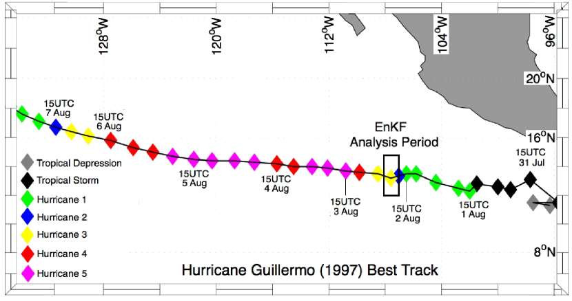
Figure 1: Best Track for Hurricane Guillermo (1997). Hurricane Intensity is color-coded based on the Saffir-Simpson scale with legend shown on the bottom left of the figure. Data courtesy of the Tropical Prediction Center (TPC), NOAA. The EnKF analysis period is denoted by the small black rectangle.

The paper is organized as follows; Section 2 first describes the predictive component of the parameter estimation model including the analytic equation set of the hurricane model, the four model parameters present within this predictive model, the discretization, and a brief overview of the EnKF data assimilation method. In Section 3 we describes various aspects of the parameter estimation model setup including the ensemble setup and the processing of the derived observational data fields. Section 4 is broken up into three sub-sections with each section showing results relating to the three major points of this paper. A summary and final remarks are presented in Section 5.

2 Parameter estimation model

The parameter estimation model is comprised of a predictive model and an parameter estimation model. The chosen predictive model is the Navier-Stokes equation set coupled to a bulk cloud model with the four parameters utilized within this model, whereas the parameter estimation model employs the EnKF data assimilation. In addition to describing their representative analytical representations, discussions regarding their respective discrete formulations will also be presented in this section.

2.a Predictive model

2.a.1 Navier-Stokes equation set

Since the analytical equation set representing the momentum, energy, and mass of the gas phase is identical to that utilized in Reisner and Jeffery (2009), RJ hereafter, interested readers can examine this manuscript for details regarding its formulation. Likewise the primary difference between the equation set found in that paper and the current equation set are additional terms associated with buoyancy in the vertical equation of motion related to various hydrometers, i.e., $g({\rho}^{\prime}+\rho_{c}+\rho_{r}+\rho_{i}+\rho_{s}+\rho_{g})$ where $g$ is gravity, ${\rho}^{\prime}$ is a density perturbation, $\rho_{c}$ is the cloud water density, $\rho_{r}$ is the rain water density, $\rho_{i}$ is the ice water density, $\rho_{s}$ is the density of snow, and $\rho_{g}$ is the graupel density, with the next section briefly describing the bulk microphysical model used to predict the evolution of the hydrometers.

2.a.2 Bulk microphysical model

The mass conservation equation for a given particle type, ${\rho}_{part}=\rho_{c},\rho_{r},\rho_{i},\rho_{s},\rho_{g}$, within the bulk microphysical model can be written as follows

$${\partial(\rho_{part})\over\partial t}+{\partial[(u^{i^{\prime}}-wfall_{part}\delta_{i^{\prime}3})\rho_{part}]\over\partial x^{i^{\prime}}}=fdensity_{part}+{\partial F^{i^{\prime}}_{\rho_{part}}\over\partial x^{i^{\prime}}},$$ (1)

where $u^{i^{\prime}}$ are fluid velocities in each spatial direction and the last term represents the turbulent diffusion of a particle type using a diffusion coefficient diagnosed from a turbulence kinetic energy (TKE) equation, see Eq. 3 in Reisner and Jeffery (2009).

The conservation equation for either cloud droplet number ($N_{c}$) or ice particle number ($N_{i}$), $N_{part}=N_{c},N_{i}$, can be written as follows

$${\partial(N_{part})\over\partial t}+{\partial[(u^{i^{\prime}}-wfall_{part}\delta_{i^{\prime}3})N_{part}]\over\partial x^{i^{\prime}}}=fnumber_{part}+{\partial F^{i^{\prime}}_{N_{part}}\over\partial x^{i^{\prime}}},$$ (2)

where $wfall_{part}$, $fdensity_{part}$, and $fnumber_{part}$ represent the fall speed, density, and number sources or sinks from the bulk microphysical model for a given particle type, a hybrid of the activation and condensation model found in Reisner and Jeffery (2009) together with all of the other relevant bulk parameterizations found in Thompson et al. (2008). Note, because of significant differences in the particle distributions between winter storms and hurricanes, the slope-intercept formulas were modified following McFarquhar and Black (2004).

2.a.3 Parameters of interest

The initialization of the environmental or background horizontal homogeneous potential temperature, water vapor, and total gas density fields for all Guillermo simulations was achieved by examining vertical profiles from ECMWF analyses obtained near the time period of the dual-Doppler radar data (1830 UTC 2 August to 0030 UTC 3 August 1997) and using a representative composite. Though some uncertainty exists within the thermodynamic fields with regard to the actual environment versus the perturbed environment obtained from the ECMWF soundings, the impact of this uncertainty was deemed to be smaller than that associated with the momentum fields, i.e., the simulated vortex is sensitive to small changes in wind shear. So to quantify this sensitivity, the horizontal velocity fields, $u^{1^{\prime}}$ and $u^{2^{\prime}}$, were initialized as follows

$$u^{1^{\prime}}(x^{3^{\prime}}) = \phi_{shear}[ecmwf_{u}(x^{3^{\prime}})+1.5],$$ (3)

$$u^{2^{\prime}}(x^{3^{\prime}}) = \phi_{shear}[ecmwf_{v}(x^{3^{\prime}})-1.5],$$ (4)

where $\phi_{shear}$ is a tuning coefficient that determines the shear impacting hurricane Guillermo within a range of 0 and 1, $x^{3^{\prime}}$ is the height, and $ecmwf_{u}$ and $ecmwf_{v}$ represent mean soundings calculated from the ECMWF analyses.

Given the delicate balance in nature that is needed for a sheared hurricane to intensify, it is not entirely obvious whether numerical models, that are necessarily limited in resolution, can accurately represent boundary processes that are responsible for supplying water vapor to eyewall convection. The accurate representation of boundary-layer processes implies the model has been somewhat “tuned” to represent the impacts of waves, sea spray, and air bubbles within the water; likewise the accurate treatment of energy release in eyewall convection implies that the upward movement of, for example, moisture is being reasonably simulated by the hurricane model.

To examine this uncertainty the diffusion coefficient for surface momentum calculations was specified as follows

$$\kappa=\kappa_{surfacefriction}\tanh\left({{\bf V_{h}}\over 80}\right),$$ (5)

where $\kappa_{surfacefriction}$ is a tuning coefficient that ranges from 0.1 to 10 m² s^-1 and ${\bf V_{h}}$ is the near surface horizontal wind speed. A no-slip boundary condition was utilized in the horizontal momentum equations ($u^{1^{\prime}}$ =$u^{2^{\prime}}$=0) with the magnitude of $\kappa_{surfacefriction}$ the determining factor with regard to the impact of this boundary condition on the intensity and structure of Guillermo. Note, unlike for the horizontal momentum equations, all scalar equations use a diffusion coefficient estimated from the $TKE$ equation within calculations of surface fluxes.

Another uncertain boundary-layer process that has a significant impact on intensification rate is surface moisture availability and the unresolved vertical transport of this water vapor with the first term, $q^{s}_{v}$, being formulated as follows

$${q^{s}_{v}}=q_{vs}\left(0.75+{q_{v}}_{surface}\right)\tanh\left({{\bf V_{h}}\over 30}\right),$$ (6)

where $q_{vs}$ is the saturated vapor pressure over water and ${q_{v}}_{surface}$ is a tuning coefficient that ranges in value from 0.0 to 0.2. This term enters into surface diffusional flux calculations of water vapor, $F^{3^{\prime}}_{q_{v}}$, in discrete form as follows

$$F^{3^{\prime}}_{q_{v}}=\kappa{{q^{1}_{v}-q^{s}_{v}}\over{0.5\Delta x^{3^{\prime}}}},$$ (7)

where $q^{1}_{v}$ is the specific humidity of the first grid cell in the vertical direction. To address the uncertainty associated with the turbulent transport of water vapor (and all other fields) from the surface to the free atmosphere the turbulent length scale was modified as follows

$$L^{m}_{s}={\phi}_{turb}L_{s},$$ (8)

where the tuning coefficient, ${\phi}_{turb}$, ranged from 0.1 to 10, and the eddy diffusivity now being $\kappa=0.09L^{m}_{s}\sqrt{TKE}$.

2.a.4 Discrete model

The discrete model for the Navier-Stokes equation set and the bulk microphysical model closely follows what was described in section 2c of RJ. This discrete equation set formulated on an A-grid can utilize a variety of time-stepping procedures with the current simulations using a semi-implicit procedure (Reisner et al. (2005)). The advection scheme used to advect gas and various cloud quantities was the quadratic upstream interpolation for convective kinematics advection scheme including estimated streaming terms (QUICKEST, Leonard and Drummond (1995)) with these quantities having the possibility of being limited by a flux-corrected transport procedure (Zalesak (1979)).

The domain spans 1200 km in either horizontal direction and 21 km in the vertical direction. The stretched horizontal mesh employing 300 grid points has the highest resolution of 1 km at the center of the mesh and lowest resolution of 7 km at the model edges. Because of the addition of a mean wind intended to keep the vortex centered in the middle of the domain, the coarsest resolution resolving the highest wind field of Guillermo is approximately 2 km. The stretched vertical mesh is resolved by 86 grid points with highest resolution of 50 m at the surface and lowest of 500 m at the model top.

2.b Parameter estimation Model

In this section the ensemble Kalman filter (EnKF) method is briefly described. In the current work, the EnKF is mainly utilized to estimate the model parameters.

2.b.1 Parameter estimation with EnKF

The ensemble Kalman Filter is a Monte Carlo approach of the Kalman filter which estimates the covariances between observed variables and the model state variables through an ensemble of predictive model forecasts. The EnKF was first introduced by Evensen (1994) and is discussed in detail in Evensen and van Leeuwen (1996) and in Houtekamer and Mitchell (1998). For the current study, only the parameters will be estimated, not the state vector of the model. The EnKF procedure is directly applied to the parameters, i.e., the state vector contains only the parameter values. Nevertheless, the model covariance matrix is still required for the innovation with observations. The following EnKF description will be concern with model parameters.

Let $\mathbf{p}\in\mathbb{R}^{\ell}$ be a vector holding the different model parameters, and $\mathbf{x}^{f}\in\mathbb{R}^{n}$ be the model state forecast. Let $\left(\mathbf{p}_{i},\mathbf{x}^{f}_{i}\right)$ for $i=1\ldots N$ be an ensemble of model parameters and state forecasts, and $\mathbf{y}^{o}\in\mathbb{R}^{m}$ a vector of $m$ observations, then the estimated parameter values $\mathbf{p}^{a}_{i}$ given by the EnKF equations are

$$\mathbf{p}^{a}_{i} = \mathbf{p}_{i}+\tilde{\mathbf{K}}\left(\mathbf{y}^{o}_{i}-\mathbf{H}\mathbf{x}^{f}_{i}\right),\qquad i=1,\ldots,N$$ (9)

$$\tilde{\mathbf{K}} = \mathbf{C}^{T}\mathbf{H}^{T}\left(\mathbf{H}\mathbf{P}^{f}\mathbf{H}^{T}+\mathbf{R}\right)^{-1},$$ (10)

where the matrix $\tilde{\mathbf{K}}\in\mathbb{R}^{\ell\times m}$ is a modified Kalman gain matrix (see Appendix A), $\mathbf{P}^{f}\in\mathbb{R}^{n\times n}$ is the model forecast covariance matrix, $\mathbf{C}\in\mathbb{R}^{n\times\ell}$ is the cross-correlation matrix between the model forecast and parameters, $\mathbf{R}\in\mathbb{R}^{m\times m}$ is the observations covariance matrix, and $\mathbf{H}\in\mathbb{R}^{m\times n}$ is an observation operator matrix that maps state variables onto observations. In the EnKF, the vector $\mathbf{y}^{o}_{i}$ is a perturbed observation vector defined as

$$\mathbf{y}^{o}_{i}=\mathbf{y}^{o}+\varepsilon_{i},$$ (11)

where $\varepsilon_{i}\in\mathbb{R}^{m}$ is a random vector sampled from a normal distribution with zero mean and a specified standard deviation $\sigma$. Usually $\sigma$ is taken as the variance or error in the observations.

One of the main advantages of the EnKF is that the model forecast covariance matrix is approximated using the ensemble of model forecasts,

$$\mathbf{P}^{f}\approx\frac{1}{N-1}\sum^{N}_{i=1}\left(\mathbf{x}^{f}_{i}-\bar{\mathbf{x}}^{f}\right)\left(\mathbf{x}^{f}_{i}-\bar{\mathbf{x}}^{f}\right)^{T},$$ (12)

where $\bar{\mathbf{x}}^{f}\in\mathbb{R}^{n}$ is the model forecast ensemble average. The use of an ensemble of model forecast to approximate $\mathbf{P}^{f}$ enables the evolution of this matrix for large non-linear models at a reasonable computational cost. Additionally, the cross-correlation matrix $\mathbf{C}$ is defined as

$$\mathbf{C}=\frac{1}{N-1}\sum^{N}_{i=1}\left(\mathbf{x}^{f}_{i}-\bar{\mathbf{x}}^{f}\right)\left(\mathbf{p}_{i}-\bar{\mathbf{p}}\right)^{T},$$ (13)

where $\bar{\mathbf{p}}\in\mathbb{R}^{\ell}$ is the parameter ensemble average.

For our particular implementation, the system of equations (9)-(10) is rewritten as

$$\left(\mathbf{H}\mathbf{P}^{f}\mathbf{H}^{T}+\mathbf{R}\right)\mathbf{z}_{i}=\left(\mathbf{y}^{o}_{i}-\mathbf{H}\mathbf{x}^{f}_{i}\right)$$ (14)

$$\mathbf{p}^{a}_{i}=\mathbf{p}_{i}+\mathbf{C}^{T}\mathbf{H}^{T}\mathbf{z}_{i},$$ (15)

for $i=1,\ldots,N$, where $\mathbf{z}_{i}\in\mathbb{R}^{m}$ is the solution of the linear system (14) for ensemble $i$. For our implementation, the observation covariance matrix $\mathbf{R}$ is taken as a diagonal matrix, with $\sigma$ in its main diagonal.

2.b.2 Considerations for parameter estimation with EnKF

Several studies have utilized the EnKF data assimilation to simultaneously estimate the model state and parameter. Among them are the studies by Aksoy et al. (2006a), Aksoy et al. (2006b), Tong and Xue (2008), Hu et al. (2010), and Nielsen-Gammon et al. (2010). Typically, the parameters are included as part of the model state in the assimilation. This evolving of dynamical and non-evolving elements within the analysis introduces some difficulties for parameter estimation, such as parameter collapse and assimilation divergence. To mitigate these difficulties, the parameters are inflated to a prespecified variance, so as to avoid the collapse and keep a reasonable spread in the parameters. These techniques have proven to be effective to estimate parameter, but they require adjustments and tuning of the inflation to obtain good estimates.

The particular approach taken in this work is to use the EnKF as a tool to only estimate the model parameters using the available data. This approach is significantly different from the studies mentioned above in the sense that only the parameters are estimated with the EnKF, that is, the model state is not being estimated. The motivation behind this approach is that model parameters are assumed to be constant, they do not evolve through the model, although they affect the dynamics of the solution. For this reason, determining parameters can be viewed as a stationary or static optimization. Our objective is to estimate a constant parameter value for the given data set, over the given time window. To achieve this, the assimilation of the data is performed on each time instance, where observations are available, independently. The reasoning behind this technique is to treat the parameters as constants and non-evolving elements in the model, hence for each time period we compute an estimated parameter value.

The procedure used to estimate the parameters is the following: Let $t_{1},\ldots,t_{k}$ be the time instances where observations are available. For each time instance $t_{j}$, $j=1,\ldots,k$, the EnKF data assimilation (equations (14)-(15)) provides parameter estimates for the ensemble, $\mathbf{p}^{a}_{i}\left(t_{j}\right)$, $i=1\ldots N$. A final parameter estimate is then computed by first taking the ensemble average and then the time average of the parameters, that is

$$\mathbf{p}^{a}=\frac{1}{k}\sum^{k}_{j=1}\left[\frac{1}{N}\sum^{N}_{i=1}\mathbf{p}^{a}_{i}\left(t_{j}\right)\right]$$ (16)

One advantage is that this approach avoids the problem of parameter collapse and filter divergence, since the data assimilation is used to estimate the parameters at each time instance independently. Additionally, since the state is not being updated in the assimilation, and only the parameter are being estimated, localization is not required for the EnKF.

The number of available data points for Hurricane Guillermo is about $200,000$ at any given time. This rich data set can be used to investigate a number of aspects of hurricane intensification. In order to exploit this data set for assimilation, we used an efficient matrix-free EnKF algorithm developed by Godinez and Moulton (in press, DOI: 10.1007/s10596-011-9268-9). The algorithm works by efficiently solving the linear system (14) using a solver based on the Sherman-Morrison formulas. In their paper, Godinez and Moulton (in press, DOI: 10.1007/s10596-011-9268-9) show that this algorithm is more efficient than traditional implementations of the EnKF, by several orders of magnitude, and enables the assimilation of vast amounts of data. Additionally, the algorithm provides an analysis that is qualitatively and quantitatively the same as more traditional implementations. The reader is referred to the work of Godinez and Moulton (in press, DOI: 10.1007/s10596-011-9268-9) for more details.

3 Parameter estimation model setup

This section describes the three necessary steps to conduct the parameter estimates: the processing of derived observational data fields; the setting up of the ensemble; and the setup of the EnKF system.

3.a Derived Doppler data fields

The primary driver of a hurricane is the release of latent heat in clouds, which arises mainly from condensation. Latent heat cannot be observed directly and instruments, such as Doppler radars, only measure the reflectivity and radial velocity of precipitation particles averaged over the pulse volume. As a result, retrievals of dynamically relevant quantities (e.g. the Cartesian wind components and latent heat) are required. Guillermo’s 3-D wind field was retrieved using a variational approach on a system of equations that includes the radar projection equations, the anelastic mass continuity equation, and a Laplacian filter (Gao et al. (1999); Reasor et al. (2009)). This wind field and estimates of the precipitation water content (derived from the reflectivity measurements) are used to retrieve the latent heat of condensation/evaporation following Guimond et al. (2011). There are two main steps in the latent heat retrieval algorithm: (1) determine the saturation state at each grid point in the radar analysis using the precipitation continuity equation; and (2) compute the magnitude of heat released using the first law of thermodynamics and the vertical velocity estimates described in Reasor et al. (2009). There are several potential sources of error in the latent heat retrievals and a detailed treatment of these errors can be found in Guimond et al. (2011). Here, we summarize the most relevant information.

The uncertainty in the latent heat retrievals reduces to uncertainties in two main fields: reflectivity and vertical velocity. Guimond et al. (2011) were able to reduce and/or document the uncertainty in these fields to a level where the latent heat retrievals have a reasonably acceptable accuracy. For example, Guimond et al. (2011) focus on the inner portion of the eyewall and often use two aircraft to construct the radar analyses (Reasor et al. (2009)), which reduce the effects of attenuation. In an attempt to correct the known calibration bias in the NOAA P-3 Tail radar reflectivity, 7 dB was added to the fields (John Gamache and Paul Reasor, personal communication). More importantly, however, the reflectivity is only used to determine the condition of saturation in the latent heat retrieval. Thus, the algorithm is not dependent on the precise value of the reflectivity rendering the retrievals somewhat insensitive to errors (Guimond et al. (2011)).

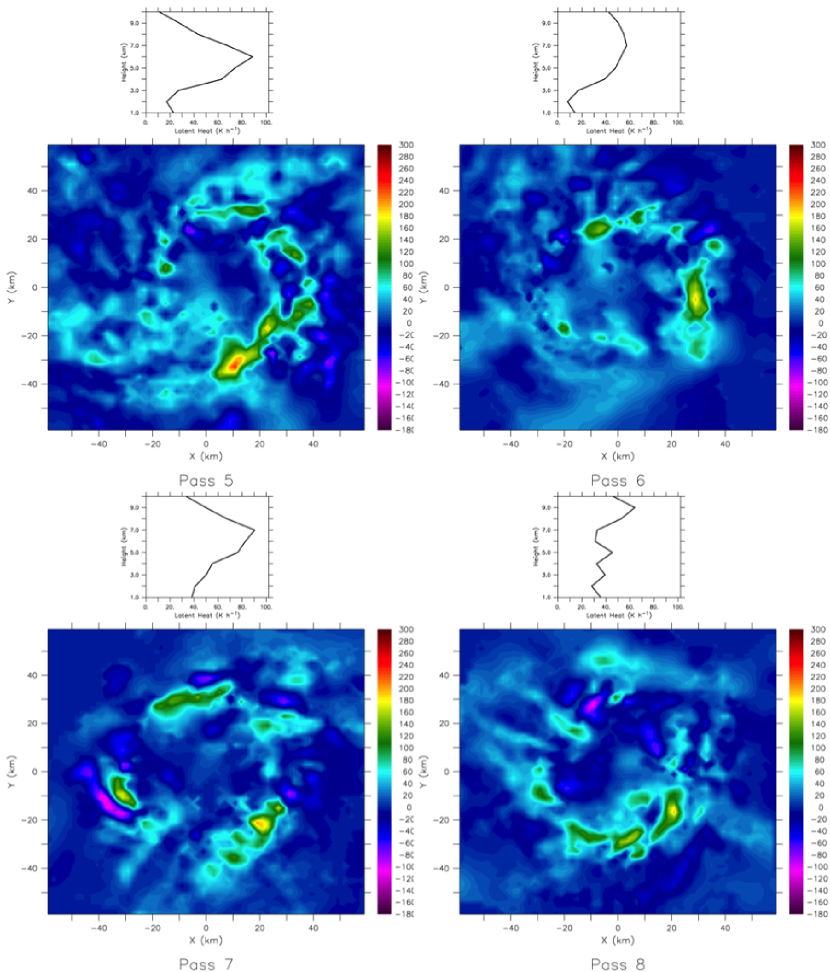
Figure 2: Horizontal views (averaged over all heights) of the latent heating rate (K h ^-1) of condensation/evaporation retrieved from airborne Doppler radar observations in Hurricane Guillermo (1997) at four select times of the dual-Doppler radar data, i.e., pass 5 corresponds to 2117 UTC from Fig. 6 of Reasor et al. (2009). Note that grid points without latent heating were assigned zero values after the vertical averaging. The vertical profile of the azimuthal mean latent heating rate at the RMW (30 km) is shown above each contour plot. The first level of data is at 1 km due to ocean surface contamination.

The uncertainties in the magnitude of the retrieved heating are dominated by errors in the vertical velocity. Using a combination of error propagation and Monte Carlo uncertainty techniques, biases are found to be small, and randomly distributed errors in the heating magnitudes are 16% for updrafts greater than 5 m s^-1 and 156% for updrafts of 1 m s ^-1 (Guimond et al. (2011)). Even though errors in the vertical velocity can lead to large uncertainties in the latent heating field for small updrafts/downdrafts, in an integrated sense, the errors are not as drastic. Figure 2 (from Guimond et al. (2011)) shows example horizontal views (averaged over all heights) of the latent heating rate of condensation/evaporation for four of the ten aircraft sampling periods of Guillermo.

For the assimilation, only latent heat data where there is a non-zero reflectivity value are incorporated into the data set. The errors for the retrieved wind fields are set to $5.0$ to $6.0$%, and the errors in the retrieved latent heating, as a percentage, are specified following Guimond et al. (2011)

$$\delta\mathbf{y}^{o}_{lh}=\left|\frac{\delta\mathbf{w}}{\mathbf{w}}\right|\times 100$$ (17)

where $\delta\mathbf{w}=1.56$ m s ^-1 represents the overall uncertainty in the vertical wind velocity field $\mathbf{w}$ Reasor et al. (2009). It is worth to notice that these errors are sometimes overestimated or underestimated. Thus in an integral sense, the errors are not so drastic, the bias is only of $+0.16$ m s ^-1.

3.b Guillermo ensemble setup

Since the primary goal is to examine the impact of various model parameters containing high uncertainty on the intensity and structure of Guillermo, but not the track, all simulations comprising the ensemble have been undertaken in which a mean wind of 1.5 m s^-1 was added or subtracted to the respective environmental wind components to prevent the movement of Guillermo from a region containing high spatial resolution found in the domain center. Specifically this high resolution patch in Cartesian space, $\Delta x^{1^{\prime}}_{c}$ and $\Delta x^{2^{\prime}}_{c}$, is defined as follows

$$\Delta x^{1^{\prime}}_{c} = 6000{\sin}^{2}({\phi}_{g}x^{*})+1000,$$ (18)

$$\Delta x^{2^{\prime}}_{c} = 6000{\sin}^{2}({\phi}_{g}y^{*})+1000,$$ (19)

where ${\phi}_{g}={\pi\over{Ngp_{i^{\prime}}}}$ determines how quickly the grid spacing changes from 7 km near the model edges to 1 km near the center with $Ngp_{i^{\prime}}$ the number of grid points in either direction and $x^{*}$,$~{}y^{*}$ represent grid values for a normalized grid with a domain employing $0.5Ngp_{i^{\prime}}$ grid points away from a center location in which $x^{*}=y^{*}=0$. Like the horizontal direction, the vertical direction also employs stretching with highest resolution near the ocean boundary, approximately 50 m, and coarsest near the model top, 500 m, with 86 vertical grid points being utilized to resolve a domain extending upwards to 21 km. Note, because of the relatively high vertical spatial resolution, time step size was limited to 1 s to avoid any instabilities associated with exceeding the advective Courant number limit.

The ensemble is generated by perturbing only the four parameters discussed in Section 2.a.3, which are ${\phi}_{shear}$, ${\kappa}_{surfacefriction}$, ${q_{v}}_{surface}$, and ${\phi}_{turb}$. The parameter values are generated by the Latin hypercube sampling technique with a uniform distribution, where each parameter is sampled over a specified interval. All ensembles have the same initial, where the background fields are initialized as described in Section 2.a.3, where the background winds that are independent of the wind field associated with Guillermo are initialized using ECMWF data. Whereas to initialize the wind field associated with Guillermo a composite of the radar winds and a bogus vortex is employed within a nudging procedure over a one hour time period. Afterwards, the hurricane model is simulated in free mode for five hours to become balanced with the parameters, and develop a hurricane vortex. It is important to mention that at this stage the behavior of the ensemble simulations are mainly dominated not by the initial conditions, but by the parameter values. Hence utilizing derived fields from the same hurricane for a vortex initialization does not bias the results of the parameter estimation experiments, as long as the subsequent spin-up is sufficiently long to allow the parameters dominate the long-term behavior of the simulation.

3.c EnKF and Observation Selection

The EnKF data assimilation is used to estimate only the parameters of interest. The time distribution of the parameters is obtained by assimilate each time period independently, as stated in Section 2.b.2. A final parameter value is obtained by averaging in time the results of the assimilation. The particular algorithm used for the parameter EnKF is a matrix-free algorithm presented in Godinez and Moulton (in press, DOI: 10.1007/s10596-011-9268-9).

parameter	interval
surface moisture	$\left[0.05,0.2\right]$
wind shear	$\left[0.1,1.0\right]$
turbulent length scale	$\left[0.1,10.0\right]$
surface friction	$\left[0.1,10.0\right]$

Table 1: Initial parameter intervals for sampling with Latin Hypercube strategy using a uniform distribution.

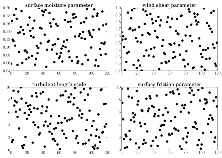
Figure 3: The parameter spread of the 120 ensemble members obtained by utilization of the Latin Hypercube sampling strategy within the limits shown in Table 1

.

The initial set of parameter values are generated using a Latin Hypercube sampling strategy with a uniform distribution. The interval for each parameter, shown in Table 1 is chosen according to the values mentioned in Section 2.a, which are based on prior sensitivity simulations and from a physical intuition of their interaction with the model. Figure 3 shows the initial distribution for each parameter of interest.

Although the optimal ensemble size for estimating reliable model uncertainty is still under active research, an ensemble of 120 members was deemed appropriate to capture essential model statistics for parameter estimation. Upon completion of the 120 member ensemble and due to the small movement of simulated hurricanes within the ensemble, information from each ensemble member was independently interpolated to the center location of the grid such to be coincident with the observations. Note, only a portion of the computational domain was utilized within the EnKF corresponding to the portion of the domain that contains the derived fields of winds and latent heat. Finally, after this interpolation step, all interpolated model and derived data fields were read into the EnKF to conduct the parameter estimation for a given time period.

The data selection procedure followed in this paper is similar to the rank parameter-observation correlation procedure presented by Tong and Xue (2008). The parameter cross-correlation matrix, $\mathbf{\mathbf{C}}$ in equation (13), provides information of the correlation between the model state variables and the parameters. By applying the observation operator $\mathbf{H}$ to the model state, we have

$$\tilde{\mathbf{C}}=\frac{1}{N-1}\sum^{N}_{i=1}\left(\mathbf{H}\mathbf{x}^{f}_{i}-\mathbf{H}\bar{\mathbf{x}}^{f}\right)\left(\mathbf{p}_{i}-\bar{\mathbf{p}}\right)^{T},$$ (20)

which is a cross-correlation matrix between parameters and model state variables in observation space. The correlations are then sorted and the observational data points that are located in regions of largest correlations are selected for assimilation. It is important to note that the regions of high correlation can be identified from different model variables fields, such as latent heat, horizontal winds, or reflectivity. This enables the use one of these fields as a proxy for observation localization in order to better capture the physical processes of interest.

4 Results

This section will highlight the three main points of this paper: 1) the highly nonlinear interactions between the various parameters leading to large variations in the simulated intensity and structure of Guillermo among the 120 ensemble members; 2) the large amounts of derived data, horizontal winds or latent heat, required to reasonably estimate the four model parameters; and 3) the newly estimated parameters lead to an overall reduction in the model forecast error.

4.a Ensemble spread and structure

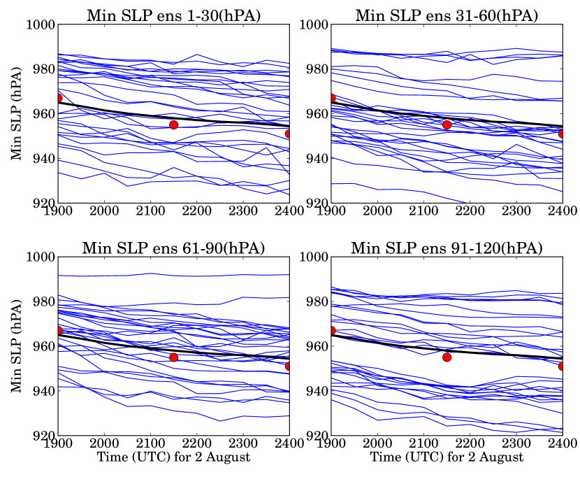
Figure 4: Minimum sea level pressure versus simulation time for each ensemble member (blue line), ensemble average (black line), and observations (red dots), for ensemble 1-30 (top left), ensemble 31-60 (top right), ensemble 61-90 (bottom left), and ensemble 91-120 (bottom right).

Since the EnKF method depends on proper model statistics to optimally determine the parameter values (Anderson (2001)) this section will illustrate this necessary variability across the various members of the ensemble. Likewise, for reasonable parameter estimation it is important that the ensemble produces statistics that are within the range of the observations and this is another aspect of the ensemble that will be presented. For example, Fig. 4 shows the simulated pressure traces for the 120 ensemble members (blue lines), the ensemble average (black line), and the 3-hourly observations from the NHC advisories (red dots) with a large spread in hurricane intensity being denoted within the ensemble. Further, even though this result may be somewhat fortuitous, the ensemble-averaged pressure trace is in remarkably good agreement with observations with a difference less than 5 hPa. To highlight differences between the ensemble average and a given member, in addition to displaying ensemble average statistics, results from a select ensemble member, i.e., member 44, that also reasonably reproduced the observed pressure trace will be shown.

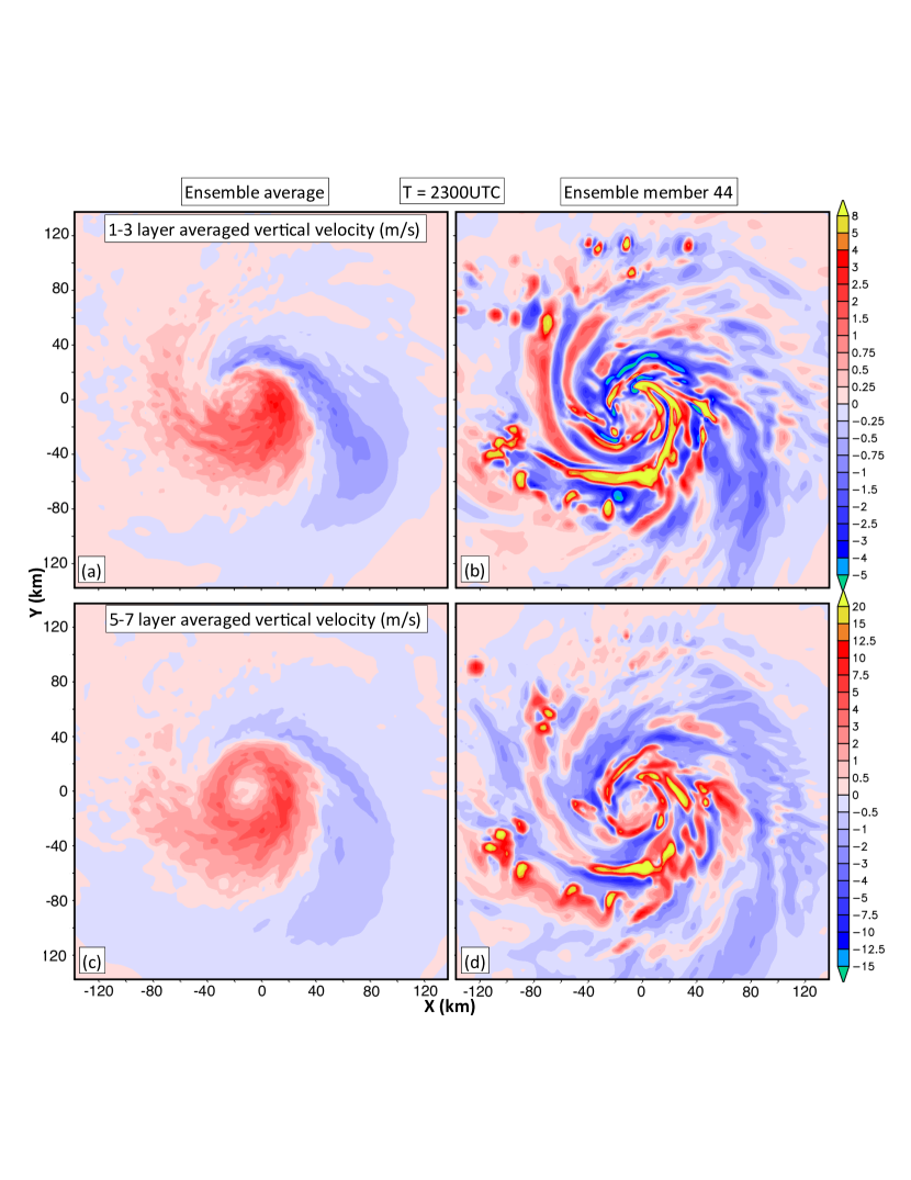
Figure 5: Ensemble average vertical motion fields at 2300 UTC (11 hours into the simulations) averaged between 1-3 km (a) or 5-7 km (c). Corresponding layer-averaged vertical motions fields from ensemble member 44 between 1-3 km (b) or 5-7 km (d).

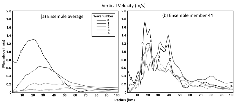
Figure 6: Time-averaged axisymmetric (black solid line) and azimuthal wavenumber-1–4 amplitudes of vertical velocity in the 1–3-km layer within a 200 km radial distance from the storm center from the ensemble average (left figure) or ensemble 44 (right figure). The averaging times are between 2230 UTC and 2300 UTC.

Because hurricane Guillermo was embedded in an environment characterized with vertical wind speed shear, its observed eyewall horizontal structure was asymmetric with a dominant wavenumber 1 mode, e.g., Reasor et al. (2009) and Sitkowski and Barnes (2009). To illustrate the models ability to reproduce this asymmetry Fig. 5 shows both the ensemble-averaged layer-averaged vertical velocities and the corresponding layer-averaged fields from member 44 at two different layers. As evident in this figure, the vortex in both the average sense and for member 44 is asymmetric with a dominant wavenumber 1 mode being readily apparent. Likewise, the impact of averaging across all members is clearly evident in Fig. 5 with a significant smoothing and reduction in vertical motions being noted with regard to the vertical motion fields produced by ensemble member 44. Furthermore, using a similar Fourier spectral decomposition procedure as Reasor et al. (2009) Fig. 6 reveals significant amounts of the vertical motion fields being in wavenumber 0 and 1 components with the magnitude of the wavenumber 1 vertical motion field from ensemble member 44 reasonably agreeing with the observations (see Fig. 15a of Reasor et al. (2009)).

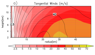
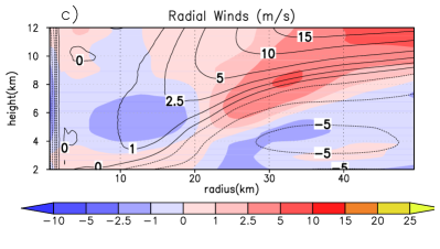
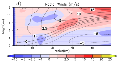
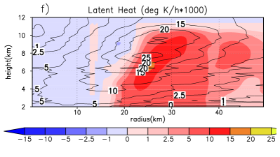
Figure 7: Comparisons between azimuthally-averaged profiles for the ensemble average (contours) and observations (shaded) for tangential winds (top), radial winds (center), and latent heat (bottom). Time periods for comparisons are at flight leg 5 (2117 UTC) and 9 (2333 UTC).

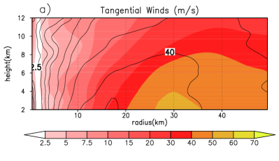
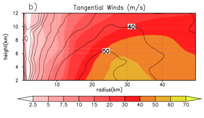
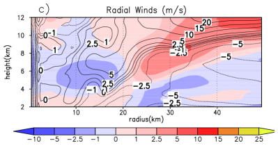
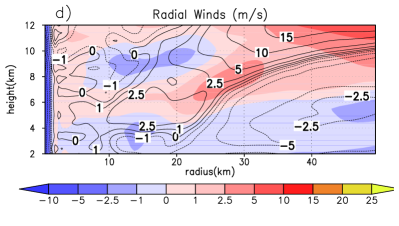
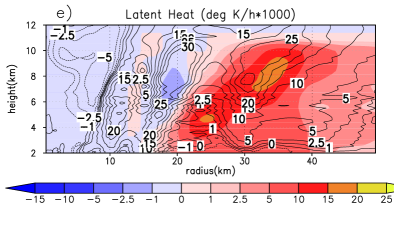
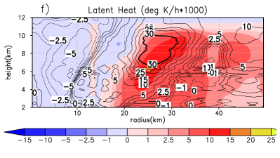
Figure 8: Comparisons between azimuthally-averaged profiles for ensemble member 44 (contours) and observations (shaded) for tangential winds (top), radial winds (center), and latent heat (bottom). Time periods for comparisons are the same as in the previous figure.

To provide another view of the simulated storm structure, both the ensemble averaged and ensemble 44 azimuthal structures were compared to observations and are presented for two flight legs in Figs. 7-8. Common disagreement with observations can be seen in both figures: First the simulated radius of maximum wind (RMW) and hence eyewall size is about $5-10$ km smaller than in the observations. While the simulated ensemble averaged azimuthal tangential component of the wind lies within $\sim 10$ m s^-1 of the observations, more notable differences are seen in the radial component of the wind with magnitudes rarely exceeding $10$ m s^-1 in the observations and the simulation consistently producing magnitudes exceeding $15$ m s^-1. Similar overestimation is produced in the latent heat fields, with values exceeding $25$ or even $30$ ($1000$ K h^-1) in the simulation with the observations showing values marginally reaching $20$ ($1000$ K h^-1).

Despite these noteworthy differences, the HIGRAD model is able to reproduce the slope/tilt of radial, tangential and latent heat fields with a reasonable degree of realism. Moreover, the heights above sea level of the contours encompassing the largest simulated values of those three fields are in overall good agreement with observations. Note, that the larger values of latent heat are required to compensate for the impact of spurious evaporation (Reisner and Jeffery (2009)) common to most cloud models with the consequences of this evaporation being discussed later in this manuscript. Additional plots were made for the remaining 8 flight legs (not shown) and displayed similar attributes.

4.b Twin-Experiments for Parameter Estimation

parameter	value
surface moisture	9.325522e-02
wind shear	4.968604e-01
turbulent length scale	3.753693
surface friction	1.443062

Table 2: Parameter values used for the reference run, from where synthetic data is used for the twin-experiments.

To asses the reliability of parameter estimation within the current context, and the amount of observational data needed for the estimation, a series of twin-experiments were performed. A synthetic observational data set is produced from a reference model run with the specific parameter values give in Table 2, and initialized according to Section 3.b. These reference parameters were selected near the ensemble average with white noise added to them.

experiment	No. obs ($m$)
TE1	20
TE2	63
TE3	200
TE4	632
TE5	2000
TE6	6325
TE7	20000
TE8	63246
TE9	200000

Table 3: Number of observations used in the twin-experiments for parameter estimation.

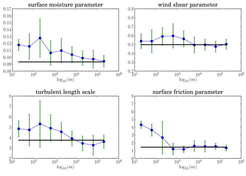
Figure 9: EnKF parameter estimation as a function of number of latent heat observations assimilated. The latent heat observations were added in locations were the ensemble is most sensitive to changes in the parameters (Section 3.c).

In their paper Tong and Xue (2008) found that to simultaneously estimate the model state and five parameters with the ensemble square root filter, using their rank parameter-observation procedure, they needed only 30 observational data points. Given that our parameter estimation setting is significantly different from their approach, it is not entirely obvious whether only small amounts of data are required to conduct the parameter estimation or, in the other limiting situation, more data than is currently available is needed for undertaking the estimates. To address this issue, nine parameter estimation experiments, named TE1 to TE9, were performed for different amounts of data, given in Table 3. The data being used for parameter estimation is the latent heat field from the reference run, where the data is selected according to the procedure described in Section 3.c. The first observation set was taken at $t=6$ hours of simulation time, afterwards nine more observation sets were taken at 30 minute intervals, which makes a total of 10 observational data set over a five hour window. For each experiment, the parameters are estimated according to Section 2.b.2, that is, parameter estimates for the ensemble are computed with the EnKF at each observational time, and then a final parameter estimate is then computed by averaging over ensemble and then time, as in equation (16). Figure 9 shows the parameter estimates for each experiment, where the vertical lines indicate the time variance of the parameter estimate. The figure clearly shows the impact of the additional data on the parameter estimates with a noticeable reduction in the error for all for parameters. Furthermore, it is only when approximately 200,000 observations are used that all four parameters converge to the correct values. This is highly relevant since it indicates that a significant amount of data is required, in this context, to correctly estimate the values of the parameters. A similar result was obtained when the horizontal wind field or reflectivity were used to estimate the parameters.

4.c Parameter Estimation Experiments with Hurricane Guillermo Observations

Given the large ensemble spread in various model fields, such as intensity, and the ability of the model to reproduce observed data suggests that estimation of the four model parameters is not only possible with the EnKF, but should produce parameter estimates that hopefully reduce model forecast errors.

The number of observations used for parameter estimation, using the EnKF in all subsequent experiment, were those identified with the highest ensemble sensitivity located at 200,000 model grid-points (see selection of observations in Section 3.c). The assimilation is performed over latent heat (DA1), horizontal winds (DA2), or both fields (DA3) started six hours into the ensemble (corresponding to 1900 UTC). With the inclusion of DA3, an assessment regarding how the EnKF procedure weights two different observational data sets and model results can be made and analyzed. Hence, this section will not only highlight how the various parameter estimates change when using different observational fields, but also how these estimates change in time.

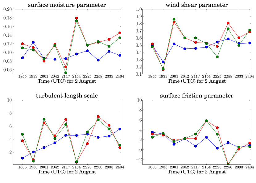
Figure 10: Time distribution of the ensemble average parameter estimates with EnKF from DA1 (blue line, latent heat), DA2 (red line, horizontal winds), and DA3 (green line, both latent heat and horizontal winds).

Figure 10 shows the time distribution of the ensemble average parameter estimates with EnKF using the 10 data time periods for DA1, DA2, and DA3. The largest temporal oscillations in the parameter estimates are associated with DA2 and suggest that the wind fields produced by the ensemble tend to oscillate more in time than the latent heat fields. Likewise, the surface moisture and the wind shear parameter estimates do not appear to change significantly in time, whereas the turbulent length scale and surface friction estimates either increase or decrease with time. Note, the temporal changes in these two parameters could be due to numerical errors and/or the impact of initial condition errors. For example, Fig. 7 shows that with time the areas of maximum latent heating and/or winds from the ensemble are expanding outward and hence this outward expansion, probably the result of numerical diffusion, could explain the temporal changes in these two parameter estimates.

parameter/simulation or DA	HG 44	DA1	DA2	DA3
surface moisture	1.944818e-01	9.431537e-02	1.189942e-01	1.132110e-01
wind shear	8.122108e-01	4.843292e-01	5.744430e-01	5.506012e-01
turbulent length scale	4.524457	3.753072	4.271998	4.401512
surface friction	2.005939	1.619931	2.120377	1.986076

Table 4: Time average parameter values for each of the experiments DA1-DA3, and the parameter values for ensemble member 44 (HG 44).

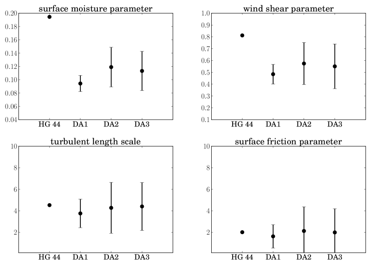
Figure 11: Analysis parameters averaged over time for ensemble member 44 (HG 44), DA1, DA2, and DA3. The vertical lines from the dots indicate the time variance of the parameter estimates each experiment.

Upon averaging the parameter estimates over the ensemble and in time, differences between the various parameter values are small; however, as will be shown in the next section these small differences in the parameters do lead to rather significant differences in both the structure and intensity of the simulated hurricanes. Table 4 show the time average parameter values from the assimilation experiments, as well as the parameter values used for ensemble member 44 prior to assimilation. Fig. 11 also reveals the various parameter estimates are different than the parameter values used in ensemble member 44, suggesting the importance of using a technique such as the EnKF to obtain the estimates, instead of simply using estimates obtained from a simulation that matches an observable such as minimum sea level pressure. This ability of the EnKF to reasonably fit the parameter values to the chosen observational data set is as well illustrated by the time averaged estimates from DA3 that, as expected, lie somewhere between the parameter estimates from DA1 and DA2, except for the turbulent length scale parameter.

4.d Parameter error assessment

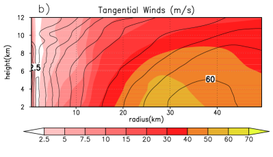
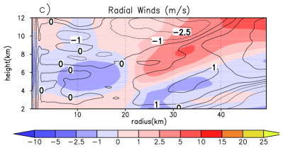
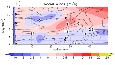
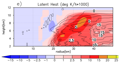
Figure 12: Comparisons of the azimuthally-averaged profiles between a model simulation (contours) using estimated parameters from DA1 and observations (color shaded). Plots for tangential winds (top), radial winds (center), and latent heat (bottom) for flight leg 5 (2117 UTC) and 9 (2333 UTC).

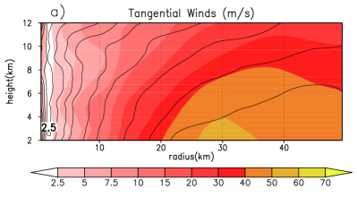
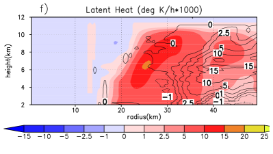
Figure 13: Comparisons of the azimuthally-averaged profiles between a model simulation using estimated parameters from DA2 and observations (color shaded). Plots for tangential winds (top), radial winds (center), and latent heat (bottom) for the same time periods as in the previous figure.

To illustrate the ability of the parameter estimates to reduce model forecast error, three simulations (SDA1, SDA2, and SDA3) were run using the time average parameter estimates from DA1, DA2, and DA3 shown in table 4. The setup for each simulation is the same as described in Subsection 3.b. Both qualitatively (see Figs. 12-13) and quantitatively (see Fig. 14) the parameter estimates produce model fields that are in better agreement with observed fields, especially the estimates associated with DA1 or those derived from using the latent heat fields. Though it is not surprising that SDA1 best matches the observed latent heat fields, what was surprising was the errors associated with the wind fields were lower in SDA1 than those associated with SDA2. This suggests the possible utility of using latent heat instead of more traditional observational fields such as horizontal winds or radar reflectivity within data assimilation procedures to estimate model parameters and/or portions of the model state vector. When a combination of both observational fields are utilized for parameter estimation, error estimates from SDA3 reveal that the response is weighted towards producing results closer to SDA2, suggesting the dominance of the horizontal wind observational data in the parameter estimates. This behavior can also be appreciated in the parameter estimates themselves, as seen in Figs. 10 and 11.

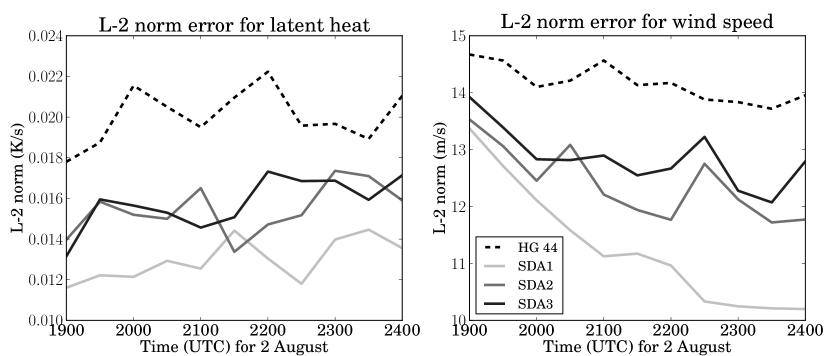
Figure 14: Error estimates as a function of time computed using Eq. 20 of Reisner and Jeffery (2009) for ensemble member 44 (HG 44), SDA1, SDA2, and SDA3.

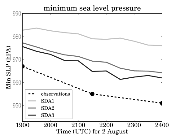
Figure 15: Minimum sea level pressure for SDA1, SDA2, and SDA3 along with the observed pressure from Hurricane Guillermo.

Though Fig. 14 demonstrates that SDA1 produces lower errors than SDA2 and SDA3, Fig. 15 illustrates that the intensity of SDA1 is significantly weaker than SDA3 and slightly weaker than SDA2. This finding may suggest that in order for SDA1 to accurately reproduce the intensity of Guillermo additional observational data is needed below the range of the radar (approximately 1 km in height) or that other errors, such as numerical errors, are contributing to the intensity differences, i.e., numerical diffusion and spurious evaporation associated with large numerical errors found near cloud boundaries. Note, like ensemble member 44, SDA2 produces nearly twice the observed amount of latent heat (see Fig. 13) suggesting the simulation is indeed having to compensate for large amounts of spurious evaporative cooling.

For example, the bottom panels of Figs. 12-13 show areas of evaporative cooling occurring immediately to the left of regions of strong positive latent heat release that do not have an analog in the observed fields. Hence, similar to what is shown in Fig. 3b of Margolin et al. (1995), this spurious cooling appears to be the result of not being able to resolve the sub-grid movement of cloud boundaries, i.e., the so-called advection-condensation problem. In fact, when a simulation using the evaporative limiter described in Reisner and Jeffery (2009) along with the parameter values from DA1 is run the resulting minimum sea level pressure from this simulation is actually slightly lower than the observed pressure (not shown). But, though SDA1 appears to suffer from relatively large numerical errors that are also common to all hurricane models, the end result of the parameter estimation procedure is still a reduction in overall model forecast error.

5 Summary and conclusions

This paper presented the estimation of key model parameters found within a hurricane model, through the use of EnKF data assimilation. The particular approach taken was to use the EnKF to only estimate the parameters at each time instance where observations were available. The advantage of this approach is that it avoids the combination of dynamic and non-dynamic elements in the assimilation procedure, which introduces difficulties when estimating parameters. An efficient matrix-free EnKF data assimilation algorithm Godinez and Moulton (in press, DOI: 10.1007/s10596-011-9268-9) is used to assimilate the derived data fields; namely horizontal wind or latent heat, available for Hurricane Guillermo. Likewise, upon completion of a 120 member ensemble that reasonably reproduced observations, the parameter estimation experiments show that a large number of data points are indeed required within the current approach to provide a reasonable estimate of the model parameters. Nevertheless, the parameter estimation procedure presented in this work can be easily be applied to other models and data sets.

A unique aspect of this work was the utilization of derived fields of latent heat to estimate the parameters. The estimates obtained using these derived fields produced lower model forecast errors than a simulation using parameter estimates obtained from horizontal wind fields or radar reflectivity alone (not shown). Unlike latent heat which can be directly linked to a simple physical process occurring within a hurricane model, i.e., condensation, utilization of other data fields such as radar reflectivity require the model to faithfully capture physical processes that are not yet well understood, i.e. collision-coalescence; and are also not the primary driver for hurricane intensification, potentially leading to large errors in parameter estimates. This result also suggests the parameters associated with the primary component of hurricane intensification, condensation of water vapor into cloud water, should also be included in the current parameter estimation procedure. It is important to note that deriving latent heat fields requires accurate vertical velocity measurements, which in most cases are not available. The availability of dual-Doppler radar data, for Hurricane Guillermo, made the computation of latent heat possible. Such a data set might not be easily acquired for other hurricanes, but one of the contributions of this work is to demonstrate the value of such a data set for parameter estimation.

Another subtle aspect suggested by this paper is that in order for a given hurricane model to both reproduce a realistic latent heat field and the correct intensity, numerical errors, especially near cloud edges, must be small. Currently, all hurricane models produce large numerical errors near cloud boundaries with these errors possibly inducing significant amounts of spurious evaporation. Hence, future work is needed to help reduce the impact of cloud-edge errors either via the calibration of a tuning coefficient employed within an evaporative limiter, i.e., see Eq. A24 in Reisner and Jeffery (2009), using the current EnKF procedure or replacing Eulerian cloud modeling approaches with a potentially more accurate Lagrangian approach (Andrejczuk et al. (2008)).

Acknowledgments. This work was supported by the Laboratory Directed Research and Development Program of Los Alamos National Laboratory, which is under the auspices of the National Nuclear Security Administration of the U.S. Department of Energy under DOE Contracts W-7405-ENG-36 and LA-UR-10-04291. Computer resources were provided both by the Computing Division at Los Alamos and the Oak Ridge National Laboratory Cray clusters. Approved for public release, LA-UR-11-10121.

APPENDIX

Appendix A: EnKF equations for parameter estimation

Many studies have used the EnKF data assimilation to simultaneously estimate model state and parameters. This can be achieved by using an augmented state vector where the parameters are appended at the end of the vector. In this appendix we review the EnKF equations for the simultaneous state and parameter estimation and extract the necessary equations for parameter estimation.

Let $\mathbf{p}\in\mathbb{R}^{\ell}$ be a vector holding the model parameters, and $\mathbf{x}^{f}\in\mathbb{R}^{n}$ be the model state forecast. Define the augmented state vector

$$\mathbf{w}=\begin{bmatrix}\mathbf{x}^{f}\\ \mathbf{p}\end{bmatrix}\in\mathbb{R}^{n+\ell}$$ (A1)

and let $\mathbf{w}_{i}$ for $i=1\ldots N$ be an ensemble of model state forecast and parameters. For a vector of $m$ observations $\mathbf{y}^{o}\in\mathbb{R}^{m}$ the EnKF analysis equations are given by

$$\mathbf{w}^{a}_{i} = \mathbf{w}_{i}+\tilde{\mathbf{K}}\left(\mathbf{y}^{o}_{i}-\mathbf{H}\mathbf{x}^{f}_{i}\right),\qquad i=1,\ldots,N$$ (A2)

$$\tilde{\mathbf{K}} = \begin{bmatrix}\mathbf{P}^{f}&\mathbf{C}\\ \mathbf{C}^{T}&\mathbf{B}\end{bmatrix}\begin{bmatrix}\mathbf{H}^{T}\\ \mathbf{0}\end{bmatrix}\left(\mathbf{H}\mathbf{P}^{f}\mathbf{H}^{T}+\mathbf{R}\right)^{-1},$$ (A3)

where $\mathbf{P}^{f}\in\mathbb{R}^{n\times n}$ is the model forecast covariance matrix, $\mathbf{B}\in\mathbb{R}^{\ell\times\ell}$ is the parameter covariance matrix, $\mathbf{C}\in\mathbb{R}^{n\times\ell}$ is the cross-correlation matrix between the model forecast and parameters, $\mathbf{R}\in\mathbb{R}^{m\times m}$ is the observations covariance matrix, $\mathbf{H}\in\mathbb{R}^{m\times n}$ is an observation operator matrix that maps state variables onto observations, and $\mathbf{y}^{o}_{i}$ is a perturbed observation vector. The parameter correlation matrix is given by

$$\mathbf{B}=\frac{1}{N-1}\sum^{N}_{i=1}\left(\mathbf{p}_{i}-\bar{\mathbf{p}}\right)\left(\mathbf{p}_{i}-\bar{\mathbf{p}}\right)^{T},$$ (A4)

and the cross-correlation matrix is give by

$$\mathbf{C}=\frac{1}{N-1}\sum^{N}_{i=1}\left(\mathbf{x}^{f}_{i}-\bar{\mathbf{x}}^{f}\right)\left(\mathbf{p}_{i}-\bar{\mathbf{p}}\right)^{T},$$ (A5)

where $\bar{\mathbf{x}}^{f}$ and $\bar{\mathbf{p}}$ are the ensemble average of the model forecast and parameters, respectively.

The system of equations (A2)-(A3) can be written as

$$\left(\mathbf{H}\mathbf{P}^{f}\mathbf{H}^{T}+\mathbf{R}\right)\mathbf{z}_{i}=\left(\mathbf{y}^{o}_{i}-\mathbf{H}\mathbf{x}^{f}_{i}\right)$$ (A6)

$$\mathbf{w}^{a}_{i}=\mathbf{w}_{i}+\begin{bmatrix}\mathbf{P}^{f}&\mathbf{C}\\ \mathbf{C}^{T}&\mathbf{B}\end{bmatrix}\begin{bmatrix}\mathbf{H}^{T}\\ \mathbf{0}\end{bmatrix}\mathbf{z}_{i},$$ (A7)

where the vector $\mathbf{z}_{i}\in\mathbb{R}^{m}$ is the solution of equation (A6). The augmented matrix in equation (A7) can be simplified as

$$\begin{bmatrix}\mathbf{P}^{f}&\mathbf{C}\\ \mathbf{C}^{T}&\mathbf{B}\end{bmatrix}\begin{bmatrix}\mathbf{H}^{T}\\ \mathbf{0}\end{bmatrix}=\begin{bmatrix}\mathbf{P}^{f}\mathbf{H}^{T}\\ \mathbf{C}^{T}\mathbf{H}^{T}\end{bmatrix},$$

so we have the following analysis update equations for the model forecast and parameters:

$$\mathbf{x}^{a}_{i} = \mathbf{x}^{f}_{i}+\mathbf{P}^{f}\mathbf{H}^{T}\mathbf{z}_{i},$$ (A8)

$$\mathbf{p}^{a}_{i} = \mathbf{p}_{i}+\mathbf{C}^{T}\mathbf{H}^{T}\mathbf{z}_{i}.$$ (A9)

The update equation (A9), together with equations (A5) and (A6), form a system that estimate the model parameters for a given data set. This is the system used in our current study.

REFERENCES

- Aksoy et al. (2006a) Aksoy, A., F. Zhang, and J. Nielsen-Gammon, 2006a: Ensemble-Based Simultaneous State and Parameter Estimation in a Two-Dimensional Sea-Breeze Model. Mon. Wea. Rev., 134, 2951–2970.
- Aksoy et al. (2006b) Aksoy, A., F. Zhang, and J. Nielsen-Gammon, 2006b: Ensemble-based simultaneous state and parameter estimation with MM5. Geophys. Res. Lett., 33, L12 801.
- Anderson (2001) Anderson, J., 2001: An ensemble adjustment Kalman filter for data assimilation. Mon. Wea. Rev., 129, 2884–2903.
- Andrejczuk et al. (2008) Andrejczuk, M., J. Reisner, B. Henson, M. Dubey, and C. Jeffery, 2008: The potential impacts of pollution on a non-drizzling stratus deck: Does aerosol number matter more than type? J. Geophys. Res, 113, D19 204,doi:10.1029.
- Annan et al. (2005) Annan, J. D., J. C. Hargreaves, N. R. Edwards, and R. Marsh, 2005: Parameter estimation in an intermediate complexity earth system model using an ensemble Kalman filter. Ocean Modelling, 8, 135 – 154.
- Evensen (1994) Evensen, G., 1994: Sequential data assimilation with a nonlinear quasi-geostrophic model using Monte Carlo methods to forecast error statistics. J. Geophys. Res., 99 (C5), 10 143–10 162.
- Evensen and van Leeuwen (1996) Evensen, G. and P. van Leeuwen, 1996: Assimilation of Geosat altimeter data for the Agulhas Current using the ensemble Kalman filter with a quasigeostrophic model. Mon. Wea. Rev., 124, 85–96.
- Gao et al. (1999) Gao, J., M. Xue, A. Shapiro, and K. Droegemeier, 1999: A variational method for the analysis of three-dimensional wind fields from two doppler radars. Mon. Wea. Rev., 127, 2128–2142.
- Godinez and Moulton (in press, DOI: 10.1007/s10596-011-9268-9) Godinez, H. and J. Moulton, in press, DOI: 10.1007/s10596-011-9268-9: An efficient matrix-free algorithm for the ensemble Kalman filter. Comput. Geosci.
- Guimond et al. (2011) Guimond, S., M. Bourassa, and P. Reasor, 2011: A Latent Heat Retrieval and Its Effects on the Intensity and Structure Change of Hurricane Guillermo (1997). Part I: The Algorithm and Observations. J. Atmos. Sci., 68, 1549–1567.
- Hacker and Snyder (2005) Hacker, J. P. and C. Snyder, 2005: Ensemble Kalman Filter Assimilation of Fixed Screen-Height Observations in a Parameterized PBL. Mon. Wea. Rev., 133, 3260–3275.
- Houtekamer and Mitchell (1998) Houtekamer, P. and H. Mitchell, 1998: Data assimilation using an ensemble Kalman filter technique. Mon. Wea. Rev., 126, 796–811.
- Hu et al. (2010) Hu, X., F. Zhang, and J. Nielsen-Gammon, 2010: Ensemble-based simultaneous state and parameter estimation for treatment of mesoscale model error: A real-data study. Geophys. Res. Lett., 37, L08 802.
- Leonard and Drummond (1995) Leonard, B. and J. Drummond, 1995: Why you should not use ‘hybrid’, ‘power-law’ or related exponential schemes for convective modeling- there are better alternatives. Int. J. Num. Meth. Fluids, 20, 421–442.
- Margolin et al. (1995) Margolin, L., J. Reisner, and P. Smolarkiewicz, 1995: Application of the volume of fluid method to the advection-condensation problem. Mon. Wea. Rev., 125, 2265–2273.
- McFarquhar and Black (2004) McFarquhar, G. and R. Black, 2004: Observations of particle size and phase in tropical cyclones: Implications for mesoscale modeling of microphysical processes. J. Atmos. Sci., 61, 777–794.
- Nielsen-Gammon et al. (2010) Nielsen-Gammon, J., X. Hu, F. Zhang, and J. Pleim, 2010: Evaluation of planetary boundary layer scheme sensitivities for the purpose of parameter estimation. Mon. Wea. Rev., 138, 3400–3417.
- Reasor et al. (2009) Reasor, P., M. Eastin, and J. Gamache, 2009: Rapidly intensifying Hurricane Guillermo (1997). Part I: Low-wavenumber structure and evolution. Mon. Wea. Rev., 137, 603–631.
- Reisner and Jeffery (2009) Reisner, J. and C. Jeffery, 2009: A smooth cloud model. Mon. Wea. Rev., 137, 1825–1843.
- Reisner et al. (2005) Reisner, J., A. Mousseau, A. Wyszogrodzki, and D. Knoll, 2005: An implicitly balanced hurricane model with physics-based preconditioning. Mon. Wea. Rev., 133, 1003–1022.
- Sitkowski and Barnes (2009) Sitkowski, M. and G. Barnes, 2009: Low-level thermodynamic, kinematic, and reflectivity fields of Hurricane Guillermo (1997) during rapid intensification. Mon. Wea. Rev., 137, 645–663.
- Thompson et al. (2008) Thompson, G., R. Rasmussen, and K. Manning, 2008: Explicit forecasts of winter precipitation using an improved bulk microphyiscs scheme. part ii: Implementation of a new snow parameterization. Mon. Wea. Rev., 136, 5095–5115.
- Tong and Xue (2008) Tong, M. and M. Xue, 2008: Simultaneous Estimation of Microphysical Parameters and Atmospheric State with Simulated Radar Data and Ensemble Square Root Kalman Filter. Part II: Parameter Estimation Experiments. Mon. Wea. Rev., 136, 1649–1668.
- Torn and Hakim (2009) Torn, R. D. and G. J. Hakim, 2009: Ensemble Data Assimilation Applied to RAINEX Observations of Hurricane Katrina (2005). Monthly Weather Review, 137, 2817–2829.
- Zalesak (1979) Zalesak, S., 1979: Fully multidimensional flux-corrected transport algorithm for fluids. J. Comput. Phys., 31, 335–362.
- Zhang et al. (2009) Zhang, F., Y. Weng, J. Sippel, Z. Meng, and C. Bishop, 2009: Cloud-resolving hurricane initialization and prediction through assimilation of Doppler radar observations with an ensemble Kalman filter. Mon. Wea. Rev., 137, 2105–2125.
- Zou et al. (2010) Zou, X., Y. Wu, and P. S. Ray, 2010: Verification of a High-Resolution Model Forecast Using Airborne Doppler Radar Analysis during the Rapid Intensification of Hurricane Guillermo. J. Appl. Meteor. Climatol., 49, 807–820.