Dynamics in Near-Potential Games

Abstract

Except for special classes of games, there is no systematic framework for analyzing the dynamical properties of multi-agent strategic interactions. Potential games are one such special but restrictive class of games that allow for tractable dynamic analysis. Intuitively, games that are “close” to a potential game should share similar properties. In this paper, we formalize and develop this idea by quantifying to what extent the dynamic features of potential games extend to “near-potential” games.

We study convergence of three commonly studied classes of adaptive dynamics: discrete-time better/best response, logit response, and discrete-time fictitious play dynamics. For better/best response dynamics, we focus on the evolution of the sequence of pure strategy profiles and show that this sequence converges to a (pure) approximate equilibrium set, whose size is a function of the “distance” from a close potential game. We then study logit response dynamics parametrized by a smoothing parameter that determines the frequency with which the best response strategy is played. Our analysis uses a Markov chain representation for the evolution of pure strategy profiles. We provide a characterization of the stationary distribution of this Markov chain in terms of the distance of the game from a close potential game and the corresponding potential function. We further show that the stochastically stable strategy profiles (defined as those that have positive probability under the stationary distribution in the limit as the smoothing parameter goes to 0) are pure approximate equilibria. Finally, we turn attention to fictitious play, and establish that in near-potential games, the sequence of empirical frequencies of player actions converges to a neighborhood of (mixed) equilibria of the game, where the size of the neighborhood increases with distance of the game to a potential game. Thus, our results suggest that games that are close to a potential game inherit the dynamical properties of potential games. Since a close potential game to a given game can be found by solving a convex optimization problem, our approach also provides a systematic framework for studying convergence behavior of adaptive learning dynamics in arbitrary finite strategic form games.

1 Introduction

The study of multi-agent strategic interactions both in economics and engineering mainly relies on the concept of Nash equilibrium. This raises the question whether Nash equilibrium makes approximately accurate predictions of the user behavior. One possible justification for Nash equilibrium is that it arises as the long run outcome of dynamical processes, in which less than fully rational players search for optimality over time. However, unless the game belongs to special (but restrictive) classes of games, such dynamics do not converge to a Nash equilibrium, and there is no systematic analysis of their limiting behavior (Jordan 1993, Fudenberg and Levine 1998, Shapley 1964).

Potential games is a class of games for which many of the simple user dynamics, such as best response dynamics and fictitious play, converge to a Nash equilibrium (Monderer and Shapley 1996b; a, Fudenberg and Levine 1998, Sandholm 2010, Young 2004). Intuitively, dynamics in potential games and dynamics in games that are “close” (in terms of the payoffs of the players) to potential games should be related. Our goal in this paper is to make this intuition precise and provide a systematic framework for studying dynamics in finite strategic form games by exploiting their relation to close potential games.

We start by illustrating via examples that this “continuity” property of limiting dynamics need not hold for arbitrary games, i.e., games that are close in terms of payoffs may have significantly different limiting behavior under simple user dynamics. Our first example focuses on better response dynamics in which at each step or strategy profile, a player (chosen consecutively or at random) updates its strategy unilaterally to one that yields a better payoff.

Example 1.1.

Consider two games with two players and payoffs given in Figure 1. The entries of these tables indexed by row X and column Y show payoffs of the players when the first player uses strategy X and the second player uses strategy Y. Let $0<\theta\ll 1$. Both games have a unique Nash equilibrium: $(B,B)$ for ${\cal G}_{1}$, and the mixed strategy profile $\left(\frac{2}{3}A+\frac{1}{3}B,\frac{\theta}{1+\theta}A+\frac{1}{1+\theta}B\right)$ for ${\cal G}_{2}$.

We consider convergence of the sequence of pure strategy profiles generated by the better response dynamics. In ${\cal G}_{1}$, the sequence converges to strategy profile $(B,B)$. In ${\cal G}_{2}$, the sequence does not converge (it can be shown that the sequence follows the better response cycle $(A,A)$, $(B,A)$, $(B,B)$ and $(A,B)$). Thus, trajectories are not contained in any $\epsilon$-equilibrium set for $\epsilon<2$.

	A	B
A	0, 1	0, 0
B	1, 0	$\theta$, 2
${\cal G}_{1}$

	A	B
A	0, 1	0, 0
B	1, 0	$-\theta$, 2
${\cal G}_{2}$

Figure 1: A small change in payoffs results in significantly different behavior for the pure strategy profiles generated by the better response dynamics.

The second example considers fictitious play dynamics, where at each step, each player maintains an (independent) empirical frequency distribution of other player’s strategies and plays a best response against it.

Example 1.2.

Consider two games with two players and payoffs given in Figure 2. Let $0<\theta\ll 1$. It can be seen that ${\cal G}_{1}$ has multiple equilibria (including pure equilibria $(A,A)$, $(B,B)$ and $(C,C)$), whereas ${\cal G}_{2}$ has a unique equilibrium given by the mixed strategy profile where both players assign $1/3$ probability to each of its strategies.

	A	B	C
A	1, 1	1, 0	0, 1
B	0, 1	1, 1	1, 0
C	1, 0	0, 1	1, 1
${\cal G}_{1}$

	A	B	C
A	$1-\theta,1-\theta$	1, 0	0, 1
B	0, 1	$1-\theta,1-\theta$	1, 0
C	1, 0	0, 1	$1-\theta,1-\theta$
${\cal G}_{2}$

Figure 2: A small change in payoffs results in significantly different behavior for the empirical frequencies generated by the fictitious play dynamics.

We focus on the convergence of the sequence of empirical frequencies generated by the fictitious play dynamics (under the assumption that initial empirical frequency distribution assigns probability $1$ to a pure strategy profile, and whenever players are indifferent between different strategies, they choose the lexicographically smaller one). In ${\cal G}_{1}$, this sequence converges to a pure equilibrium starting from any pure strategy profile. In ${\cal G}_{2}$, the sequence displays oscillations similar to those seen in the Shapley game (see Shapley (1964), Fudenberg and Levine (1998)). To see this, assume that the initial empirical frequency distribution assigns probability 1 to the strategy profile $(A,A)$. Observe that since the underlying game is a symmetric game, empirical frequency distribution of each player will be identical at all steps. Starting from $(A,A)$, both players update their strategy to $C$. After sufficiently many updates, the empirical frequency of $A$ falls below $\theta/(1+\theta)$, and that of $C$ exceeds $1/(1+\theta)$. Thus, the payoff specifications suggest that both players start using strategy $B$. Similarly, after empirical frequency of $B$ exceeds $1/(1+\theta)$, and that of $C$ falls below $\theta/(1+\theta)$, then both players start playing $A$. Observe that update to a new strategy takes place only when one of the strategies is being used with very high probability (recall that $\theta\ll 1$) and this feature of empirical frequencies is preserved throughout. For this reason the sequence of empirical frequencies does not converge to $(1/3,1/3,1/3)$, the unique Nash equilibrium of ${\cal G}_{2}$.

In this paper, in contrast with the preceding examples, we will show that games that are close (in terms of payoffs of players) to potential games have similar limiting dynamics to those in potential games. In particular, many reasonable adaptive dynamics “converge” to an approximate equilibrium set, whose size is a function of the distance of the game to a close potential game. Our approach relies on using the potential function of a close potential game for the analysis of commonly studied update rules. We note that our results hold for arbitrary strategic form games, however our characterization of limiting behavior of dynamics is more informative for games that are close to potential games. We therefore focus our investigation to such games in this paper and refer to them as near-potential games.

We start our analysis by introducing maximum pairwise difference, a measure of “closeness” of games. Let p and q be two strategy profiles, which differ in the strategy of a single player, say player $m$. We refer to the change in the payoff of player $m$ between these two strategy profiles, as the pairwise comparison of p and q. Intuitively, this quantity captures how much player $m$ can improve its utility by unilaterally deviating from strategy profile p to strategy profile q. For given games, the maximum pairwise difference is defined as the maximum difference between the pairwise comparisons of these games. Thus, the maximum pairwise difference captures how different two games are in terms of the utility improvements due to unilateral deviations. Since equilibria of games, and strategy updates in various update rules (such as better/best response dynamics) can be expressed in terms of unilateral deviations, maximum pairwise difference provides a measure of strategic similarities of games. We show that the closest potential game to a given game, in the sense of maximum pairwise difference, can be obtained by solving a convex optimization problem. This provides a systematic way of approximating a given game with a potential game that has a similar equilibrium set and dynamic properties, as illustrated in Example 1.3.

Example 1.3.

Consider a two-player game $\cal G$, which is not a potential game, and the closest potential game to this game (in terms of maximum pairwise difference), $\hat{\cal G}$, given in Figure 3. The maximum pairwise difference of these games is $2$, since the utility improvements in these games due to unilateral deviations differ by at most $2$ (For instance consider the deviation of the column player from $(A,A)$ to $(A,B)$. In $\cal G$ this leads to a utility improvement of $6$, whereas, in $\hat{G}$ the improvement amount is $4$). It can be seen that for both games $(B,B)$ is the unique equilibrium. Moreover, trajectories of better response dynamics and empirical frequencies of fictitious play dynamics converge to this equilibrium in both games.

	A	B
A	8, 2	8, 8
B	2, 2	12, 10
${\cal G}$

	A	B
A	7, 3	9, 7
B	3, 1	11, 11
$\hat{\cal G}$

Figure 3: A game ($\cal G$) and a nearby potential game ($\hat{\cal G}$) share similar equilibrium set and dynamic properties.

We focus on three commonly studied user dynamics: discrete-time better/best response, logit response, and discrete-time fictitious play dynamics, and establish different notions of convergence for each. We first study better/best response dynamics. It is known that the sequence of pure strategy profiles, which we refer to as trajectories, generated by these update rules converge to pure Nash equilibria in potential games (Monderer and Shapley 1996b, Young 2004). In near-potential games, a pure Nash equilibrium need not even exist. For this reason we focus on the notion of pure approximate equilibria or $\epsilon$-equilibria, and show that in near-potential games trajectories of these update rules converge to a pure approximate equilibrium set. The size of this set only depends on the distance of the original game from a potential game, and is independent of the payoffs in the original game.

We then focus on logit response dynamics. With this update rule, agents, when updating their strategies, choose their best responses with high probability, but also explore other strategies with a nonzero probability. Logit response induces a Markov chain on the set of pure strategy profiles. The stationary distribution of this Markov chain is used to explain the limiting behavior of this update rule (Young 1993, Blume 1997; 1993, Alós-Ferrer and Netzer 2010, Marden and Shamma 2008). In potential games, the stationary distribution can be expressed in closed form in terms of the potential function of the game. Additionally, the stochastically stable strategy profiles, i.e., the strategy profiles which have nonzero stationary distribution as the exploration probability goes to zero, are those that maximize the potential function (Alós-Ferrer and Netzer 2010, Blume 1997, Marden and Shamma 2008). Exploiting their relation to close potential games, we obtain similar results for near-potential games: (i) we obtain an explicit characterization of the stationary distribution in terms of the distance of the game from a close potential game and the corresponding potential function, and (ii) we show that the stochastically stable strategy profiles are the strategy profiles that approximately maximize the potential of a close potential game, implying that they are pure approximate equilibria of the game. Our analysis relies on a novel perturbation result for Markov chains (see Theorem 5.1) which provides bounds on deviations from a stationary distribution when transition probabilities of a Markov chain are multiplicatively perturbed, and therefore may be of independent interest.

A summary of our convergence results on better/best response and logit response dynamics can be found in Table 1.

Update Rule	Convergence Result
Better/Best Response Dynamics	(Theorem 4.1) Trajectories of dynamics converge to ${\cal X}_{\delta h}$, i.e., the $\delta h$-equilibrium set of $\cal G$.
Logit Response Dynamics (with parameter $\tau$)	(Corollary 5.2) Stationary distribution $\mu_{\tau}$ of logit response dynamics is such that $\left|\mu_{\tau}({\mathbf{p}})-\frac{e^{\frac{1}{\tau}\phi(\mathbf{p})}}{\sum_{\mathbf{q}\in E}e^{\frac{1}{\tau}\phi(\mathbf{q})}}\right|\leq\frac{e^{\frac{2\delta(h-1)}{\tau}}-1}{e^{\frac{2\delta(h-1)}{\tau}}+1}$, for all $\mathbf{p}$.
Logit Response Dynamics	(Corollary 5.3) Stochastically stable strategy profiles of $\cal G$ are (i) contained in $S=\{\mathbf{p}|\phi(\mathbf{p})\geq\max_{\mathbf{q}}\phi(\mathbf{q})-4\delta(h-1)\}$, (ii) $4\delta h$-equilibria of $\cal G$.

Table 1: Convergence properties of better/best response and logit response dynamics in near-potential games. Given a game $\cal G$, we use $\hat{\cal G}$ to denote a nearby potential game with potential function $\phi$ such that the distance (in terms of the maximum pairwise difference, defined in Section 2) between the two games is $\delta$. We use the notation ${\cal X}_{\epsilon}$ to denote the $\epsilon$-equilibrium set of the original game, $h$ to denote the number of strategy profiles, $\mu_{\tau}$ and $\hat{\mu}_{\tau}$ to denote the stationary distributions of logit response dynamics in $\cal G$ and $\hat{\cal G}$, respectively.

We finally analyze fictitious play dynamics in near-potential games. In potential games trajectories of fictitious play need not converge to a Nash equilibrium, but the empirical frequencies of the played strategies converge to a (mixed) Nash equilibrium (Monderer and Shapley 1996a, Shamma and Arslan 2004). In our analysis of fictitious play dynamics, we first show that in near-potential games if the empirical frequencies are outside some $\epsilon$-equilibrium set, then the potential of the close potential game (evaluated at the empirical frequency distribution) increases with each strategy update. Using this result we establish convergence of fictitious play dynamics to a set which can be characterized in terms of the $\epsilon$-equilibrium set of the game and the level sets of the potential function of a close potential game. This result suggests that in near-potential games, the empirical frequencies of fictitious play converge to a set of mixed strategies that (in the close potential game) have potential almost as large as the potential of Nash equilibria. Moreover, exploring the property that for small $\epsilon$, $\epsilon$-equilibria are contained in disjoint neighborhoods of equilibria, we strengthen our result and establish that if a game is sufficiently close to a potential game, then empirical frequencies of fictitious play dynamics converge to a small neighborhood of equilibria. This result recovers as a special case convergence of empirical frequencies to Nash equilibria in potential games.

A summary of our results on convergence of fictitious play dynamics is given in Table 2.

Update Rule	Convergence Result
Fictitious Play	(Corollary 6.1) Empirical frequencies of dynamics converge to the set of mixed strategies with large enough potential: $\{\mathbf{x}\in\prod_{m}\Delta E^{m}|\phi(\mathbf{x})\geq\min_{\mathbf{y}\in{\cal X}_{M\delta}}\phi(\mathbf{y})\}$
Fictitious Play	(Theorem 6.2) Assume that $\cal G$ has finitely many equilibria. There exists some $\bar{\delta}>0$, and $\bar{\epsilon}>0$ (which are functions of utilities of $\cal G$ but not $\delta$) such that if $\delta<\bar{\delta}$, then the empirical frequencies of fictitious play converge to {x —   —— x -x_k—— ≤4f(Mδ) MLϵ +f(Mδ+ϵ), for some equilibrium $\mathbf{x}_{k}$ }, for any $\epsilon$ such that $\bar{\epsilon}\geq\epsilon>0$, where $f:\mathbb{R}_{+}\rightarrow\mathbb{R}_{+}$ is an upper semicontinuous function such that $f(x)\rightarrow 0$ as $x\rightarrow 0$.

Table 2: Convergence properties of fictitious play dynamics in near-potential games. We denote the number of players in the game by $M$, set of mixed strategies of player $m$ by $\Delta E^{m}$, and the Lipschitz constant of the mixed extension of $\phi$ by $L$. Rest of the notation is the same as in Table 1.

The framework provided in this paper enables us to study the limiting behavior of adaptive user dynamics in arbitrary finite strategic form games. In particular, for a given game we can use the proposed convex optimization formulation to find a nearby potential game and use the distance between these games to obtain a quantitative characterization of the limiting approximate equilibrium set. The characterization this approach provides will be tighter if the original game is closer to a potential game.

Related Literature: Potential games play an important role in game-theoretic analysis because of existence of pure strategy Nash equilibrium, and the stability (under various learning dynamics such as better/best response dynamics) of pure Nash equilibria in these games (Monderer and Shapley 1996b, Fudenberg and Levine 1998, Young 2004). Because of these properties, potential games found applications in various control and resource allocation problems (Monderer and Shapley 1996b, Marden et al. 2009a, Candogan et al. 2010a, Arslan et al. 2007).

There is no systematic framework for analyzing the limiting behavior of many of the adaptive update rules in general games (Jordan 1993, Fudenberg and Levine 1998, Shapley 1964). However, for potential games there is a long line of literature establishing convergence of natural adaptive dynamics such as better/best response dynamics (Monderer and Shapley 1996b, Young 2004), fictitious play (Monderer and Shapley 1996a, Shamma and Arslan 2004, Marden et al. 2009b, Hofbauer and Sandholm 2002) and logit response dynamics (Blume 1993; 1997, Alós-Ferrer and Netzer 2010, Marden and Shamma 2008).

It was shown in recent work that a close potential game to a given game can be obtained by solving a convex optimization problem (see Candogan et al. (2011; 2010b)). It was also proved that equilibria of a given game can be characterized by first approximating this game with a potential game, and then using the equilibrium properties of close potential games (Candogan et al. 2011; 2010b). This paper builds on this line of work to study dynamics in games by exploiting their relation to a close potential game.

Paper Organization: The rest of the paper is organized as follows: We present the game theoretic preliminaries for our work in Section 2. In Section 3, we explain how a close potential game to a given game can be found, and discuss possible extensions of this approach. We present an analysis of better and best response dynamics in near-potential games in Section 4. In Section 5, we extend our analysis to logit response, and focus on the stationary distribution and stochastically stable stable states of logit response. We present the results on fictitious play, and its extensions in Section 6. We close in Section 7 with concluding remarks and future work.

2 Preliminaries

In this section, we present the game-theoretic background that is relevant to our work. Additionally, we introduce the closeness measure for games, which is used in the rest of the paper.

2.1 Finite Strategic Form Games

Our focus in this paper is on finite strategic form games. A (noncooperative) finite game in strategic form consists of:

• A finite set of players, denoted by ${\cal M}=\{1,\dots,M\}$.

• Strategy spaces: A finite set of strategies (or actions) $E^{m}$, for every $m\in{\cal M}$.

• Utility functions: $u^{m}:\prod_{k\in{\cal M}}E^{k}\rightarrow{\mathbb{R}}$, for every $m\in{\cal M}$.

We denote a (strategic form) game instance by the tuple $\langle{\cal M},\{E^{m}\}_{m\in{\cal M}},\{u^{m}\}_{m\in{\cal M}}\rangle$, and the joint strategy space of this game instance by $E=\prod_{m\in{\cal M}}E^{m}$. We refer to a collection of strategies of all players as a strategy profile and denote it by $\textbf{p}=({p}^{1},\dots,{p}^{M})\in E$. The collection of strategies of all players but the $m$th one is denoted by $\textbf{p}^{-m}$.

The basic solution concept in a noncooperative game is that of a Nash Equilibrium (NE). A (pure) Nash equilibrium is a strategy profile from which no player can unilaterally deviate and improve its payoff. Formally, ${\bf p}$ is a Nash equilibrium if

$$u^{m}({q}^{m},{\bf p}^{-m})-u^{m}({p}^{m},{\bf p}^{-m})\leq 0,$$

for every ${{q}^{m}\in E^{m}}$ and $m\in\mathcal{M}$.

To address strategy profiles that are approximately a Nash equilibrium, we use the concept of $\epsilon$-equilibrium. A strategy profile ${\bf p}\triangleq({{p}}^{1},\dots,{{p}}^{M})$ is an $\epsilon$-equilibrium ($\epsilon\geq 0$) if

$$u^{m}({q}^{m},{\bf p}^{-m})-u^{m}({p}^{m},{{\bf p}}^{-m})\leq\epsilon$$

for every ${{q}^{m}\in E^{m}}$ and $m\in\mathcal{M}$. We denote the set of $\epsilon$-equilibria in a game $\cal G$ by ${\cal X}_{\epsilon}$. Note that a Nash equilibrium is an $\epsilon$-equilibrium with $\epsilon=0$.

2.2 Potential Games

We next describe a particular class of games that is central in this paper, the class of potential games (Monderer and Shapley 1996b).

Definition 2.1 (Potential Game).

A potential game is a noncooperative game for which there exists a function $\phi:E\rightarrow\mathbb{R}$ satisfying

$$u^{m}({p}^{m},{\bf p}^{-m})-u^{m}({q}^{m},{\bf p}^{-m})=\phi({p}^{m},{\bf p}^{-m})-\phi({q}^{m},{\bf p}^{-m}),$$ (1)

for every $m\in{\cal M}$, ${p}^{m},{q}^{m}\in E^{m}$, ${\bf p}^{-m}\in E^{-m}$. The function $\phi$ is referred to as a potential function of the game.

This definition ensures that the change in the utility of a player who unilaterally deviates to a new strategy, coincides exactly with the corresponding change in the potential function. Extensions of this definition in which equation (1) holds when each utility function is multiplied with a (possibly different) positive weight, or changes in utility and potential only agree in sign, give rise to weighted and ordinal potential games that share similar properties to potential games. We briefly discuss some of these extensions in Section 3. However, our main focus in this paper is on potential games in Definition 2.1.

Some properties that are specific to potential games are evident from the definition. For instance, it can be seen that unilateral deviations from a strategy profile that maximizes the potential function (weakly) decrease the utility of the deviating player. Hence, this strategy profile corresponds to a Nash equilibrium, and it follows that every potential game has a pure Nash equilibrium.

Another important property of potential games, which will be used for characterizing the limiting behavior of dynamics in near-potential games, is that the total unilateral utility improvement around a “closed path” is equal to zero. Before we formally state this result, we first provide some necessary definitions, which are also used in Section 4 when we analyze better/best response dynamics in near-potential games.

Definition 2.2 (Path – Closed Path – Improvement Path).

A path is a collection of strategy profiles $\gamma=({{\bf p}}_{0},\dots{\bf p}_{N})$ such that ${{\bf p}}_{i}$ and ${{\bf p}}_{i+1}$ differ in the strategy of exactly one player. A path is a closed path (or a cycle) if ${{\bf p}}_{0}={{\bf p}}_{N}$. A path is an improvement path if $u^{m_{i}}({\bf p}_{i})\geq u^{m_{i}}({\bf p}_{i-1})$ where $m_{i}$ is the player who modifies its strategy when the strategy profile is updated from ${\bf p}_{i-1}$ to ${\bf p}_{i}$.

The transition from strategy profile ${{\bf p}}_{i-1}$ to ${{\bf p}}_{i}$ is referred to as step $i$ of the path. The length of a path is equal to its number of steps, i.e., the length of the path $\gamma=({{\bf p}}_{0},\dots,{{\bf p}}_{N})$ is $N$. We say that a closed path is simple if no strategy profile other than the first and the last strategy profiles is repeated along the path. For any path $\gamma=({{\bf p}}_{0},\dots,{{\bf p}}_{N})$ let $I(\gamma)$ represent the total utility improvement along the path, i.e.,

$$I(\gamma)=\sum_{i=1}^{N}u^{m_{i}}({{\bf p}}_{i})-u^{m_{i}}({{\bf p}}_{i-1}),$$

where $m_{i}$ is the index of the player that modifies its strategy in the $i$th step of the path. The following proposition provides a necessary and sufficient condition under which a given game is a potential game.

Proposition 2.1 (Monderer and Shapley (1996b)).

A game is a potential game if and only if $I(\gamma)=0$ for all simple closed paths $\gamma$.

We conclude this section by formally defining the measure of “closeness” of games, used in the subsequent sections.

Definition 2.3 (Maximum Pairwise Difference).

Let $\cal G$ and $\hat{\cal G}$ be two games with set of players $\cal M$, set of strategy profiles $E$, and collections of utility functions $\{u^{m}\}_{m\in{\cal M}}$ and $\{\hat{u}^{m}\}_{m\in{\cal M}}$ respectively. The maximum pairwise difference (MPD) between these games is defined as

$$d({\cal G},\hat{\cal G})\stackrel{{\scriptstyle\bigtriangleup}}{{=}}\max_{\mathbf{p}\in E,m\in{\cal M},q^{m}\in E^{m}}\left|\left(u^{m}(q^{m},\textbf{p}^{-m})-u^{m}(p^{m},\textbf{p}^{-m})\right)-\left(\hat{u}^{m}(q^{m},\textbf{p}^{-m})-\hat{u}^{m}(p^{m},\textbf{p}^{-m})\right)\right|.$$

Note that the pairwise difference $u^{m}(q^{m},\textbf{p}^{-m})-u^{m}(p^{m},\textbf{p}^{-m})$ quantifies how much player $m$ can improve its utility by unilaterally deviating from strategy profile $(p^{m},\textbf{p}^{-m})$ to strategy profile $(q^{m},\textbf{p}^{-m})$. Thus, the MPD captures how different two games are in terms of the utility improvements due to unilateral deviations. We refer to pairs of games with small MPD as close games, and games that have a small MPD to a potential game as near-potential games.

The MPD measures the closeness of games in terms of the difference of unilateral deviations, rather than the difference of their utility functions, i.e., quantities of the form

$$\left|\left(u^{m}(q^{m},\textbf{p}^{-m})-u^{m}(p^{m},\textbf{p}^{-m})\right)-\left(\hat{u}^{m}(q^{m},\textbf{p}^{-m})-\hat{u}^{m}(p^{m},\textbf{p}^{-m})\right)\right|$$

are used to identify close games, rather than quantities of the form $\left|u^{m}(p^{m},\textbf{p}^{-m})-\hat{u}^{m}(p^{m},\textbf{p}^{-m})\right|$. This is because the difference in unilateral deviations provides a better characterization of the strategic similarities (equilibrium and dynamic properties) between two games than the difference in utility functions. This can be seen from the following example: Consider two games with utility functions $\{u^{m}\}$ and $\{u^{m}+1\}$, i.e., in the second game players receive an additional payoff of $1$ at all strategy profiles. It can be seen from the definition of Nash equilibrium that despite the difference of their utility functions, these two games share the same equilibrium set. Intuitively, since the additional payoff is obtained at all strategy profiles, it does not affect any of the strategic considerations in the game. While the utility differences between these games is nonzero, it can be seen that the MPD is equal to zero. Hence MPD identifies a strategic equivalence between these games. The recent work Candogan et al. (2011) contains a formal treatment of strategic equivalence and its implications for strategic form games.

3 Finding Near-Potential Games

In this section, we present a framework for finding the closest potential game to a given game, where the distance between the games is measured in terms of MPD. We formulate the problem of identifying such a game as a convex optimization problem, and discuss the extensions of this approach. We note that a procedure for finding near-potential games can be found in Candogan et al. (2011) and Candogan et al. (2010b). In these works the distance between games is measured in terms of a 2-norm. In this section we illustrate how similar ideas can be used when the distance is measured in terms of MPD.

It can be seen from Proposition 2.1 that a game is a potential game if and only if it satisfies linear equalities. This suggests that the set of potential games is convex, i.e., if ${\cal G}=\langle{\cal M},E,\{u^{m}\}_{m}\rangle$ and $\hat{\cal G}=\langle{\cal M},E,\{\hat{u}^{m}\}_{m}\rangle$ are potential games, then ${\cal G}_{\alpha}=\langle{\cal M},E,\{\alpha{u}^{m}+(1-\alpha)\hat{u}^{m}\}_{m}\rangle$, is also a potential game provided that $\alpha\in[0,1]$.

Assume that a game with utility functions $\{u^{m}\}_{m}$ is given. The closest potential game (in terms of MPD) to this game, with payoff functions $\{\hat{u}^{m}\}_{m}$, and potential function $\phi$ can be obtained by solving the following optimization problem:

$$(\mbox{P}:)\quad\begin{aligned} \min_{\phi,\{\hat{u}^{m}\}_{m}}\quad&\max_{\mathbf{p}\in E,m\in{\cal M},q^{m}\in E^{m}}\left|\left(u^{m}(q^{m},\mathbf{p}^{-m})-u^{m}(p^{m},\mathbf{p}^{-m})\right)\right.\\ &\qquad\qquad\qquad\qquad\qquad\left.-\left(\hat{u}^{m}(q^{m},\mathbf{p}^{-m})-\hat{u}^{m}(p^{m},\mathbf{p}^{-m})\right)\right|\\ s.t.\quad&\phi(\bar{q}^{m},\bar{\mathbf{p}}^{-m})-\phi(\bar{p}^{m},\bar{\mathbf{p}}^{-m})=\hat{u}^{m}(\bar{q}^{m},\bar{\mathbf{p}}^{-m})-\hat{u}^{m}(\bar{p}^{m},\bar{\mathbf{p}}^{-m}),\\ &\mbox{for all $m\in{\cal M},~{}\bar{\mathbf{p}}\in E,~{}\bar{q}^{m}\in E^{m}$.}\end{aligned}$$

Note that the difference $\left(u^{m}(q^{m},\mathbf{p}^{-m})-u^{m}(p^{m},\mathbf{p}^{-m})\right)-\left(\hat{u}^{m}(q^{m},\mathbf{p}^{-m})-\hat{u}^{m}(p^{m},\mathbf{p}^{-m})\right)$ is linear in $\{\hat{u}^{m}\}_{m}$. Thus, the objective function is the maximum of such linear functions, and hence is convex in $\{\hat{u}^{m}\}_{m}$. The constraints of this optimization problem guarantee that the game with payoff functions $\{\hat{u}^{m}\}_{m}$ is a potential game with potential $\phi$. Note that these constrains are linear. Therefore, it follows that (P) is a convex optimization problem that gives the closest potential game to a given game.

Let ${\cal G}_{1}$ and ${\cal G}_{2}$ be games with utility functions $\{u^{m}\}_{m}$ and $\{w^{m}u^{m}\}_{m}$ respectively, where for all $m\in{\cal M}$, $w^{m}\geq 1$ is a fixed weight. It can be seen that preferences of players are identical in these two games, i.e., $u^{m}(x^{m},x^{-m})-u^{m}(y^{m},x^{-m})>0$ if and only if $w^{m}u^{m}(x^{m},x^{-m})-w^{m}u^{m}(y^{m},x^{-m})>0$ for any $m\in{\cal M}$, $y^{m}\in\Delta E^{m}$ and $\mathbf{x}\in\prod_{k\in{\cal M}}\Delta E^{k}$. Thus, it follows that the equilibrium sets of these game are the same, and for many of the update rules in games, such as better/best response dynamics, and fictitious play (but not logit response), the trajectories of dynamics in ${\cal G}_{1}$ and ${\cal G}_{2}$ are identical.

This observation suggests that it may also be of interest to find a close potential game to a “scaled version” of a given game. The following optimization formulation obtains such a potential game:

$$(\mbox{P2}:)\quad\begin{aligned} \min_{\phi,\{\hat{u}^{m}\}_{m},\{w^{m}\}_{m}}\quad&\max_{\mathbf{p}\in E,m\in{\cal M},q^{m}\in E^{m}}\left|w^{m}\left(u^{m}(q^{m},\mathbf{p}^{-m})-u^{m}(p^{m},\mathbf{p}^{-m})\right)\right.\\ &\qquad\qquad\qquad\qquad\qquad\left.-\left(\hat{u}^{m}(q^{m},\mathbf{p}^{-m})-\hat{u}^{m}(p^{m},\mathbf{p}^{-m})\right)\right|\\ s.t.\quad&w^{m}\geq 1\quad\mbox{for all $m\in{\cal M}$,}\\ \quad&\phi(\bar{q}^{m},\bar{\mathbf{p}}^{-m})-\phi(\bar{p}^{m},\bar{\mathbf{p}}^{-m})=\hat{u}^{m}(\bar{q}^{m},\bar{\mathbf{p}}^{-m})-\hat{u}^{m}(\bar{p}^{m},\bar{\mathbf{p}}^{-m}),\\ &\mbox{for all $m\in{\cal M},~{}\bar{\mathbf{p}}\in E,~{}\bar{q}^{m}\in E^{m}$.}\end{aligned}$$

The solution of (P2) is a potential game with utility functions $\{\hat{u}^{m}\}_{m}$. Comparing (P) and (P2) it can be seen that (P2) obtains the closest potential game (in terms of MPD) to the game with utility functions $\{w^{m}{u}^{m}\}_{m}$. Since (P2) also minimizes the objective function over $\{w^{m}\}$, the solution also reveals the “scaling” of the original game, which makes it as close as possible to a potential game.

In the rest of the paper, we do not discuss how a close potential game to a given game is obtained, but we just assume that a close potential game with potential $\phi$ is known and the MPD between this game and the original game is $\delta$. We provide characterization results on limiting dynamics for a given game in terms of $\phi$ and $\delta$.

4 Better Response and Best Response Dynamics

In this section, we consider better and best response dynamics, and study convergence properties of these update rules in near-potential games. All of the update rules considered in this section are discrete-time update rules, i.e., players are allowed to update their strategies at time instants $t\in\mathbb{Z}_{+}=\{1,2,\dots\}$.

Best response dynamics is an update rule where at each time instant a player chooses its best response to other players’ current strategy profile. In better response dynamics, on the other hand, players choose strategies that improve their payoffs, but these strategies need not be their best responses. Formal descriptions of these update rules are given below.

Definition 4.1 (Better and Best Response Dynamics).

At each time instant $t\in\{1,2,\dots\}$, a single player is chosen at random for updating its strategy, using a probability distribution with full support over the set of players. Let $m$ be the player chosen at some time $t$, and let $\textbf{r}\in E$ denote the strategy profile that is used at time $t-1$.

1. Better response dynamics is the update process where player $m$ does not modify its strategy if $u^{m}(\mathbf{r})=\max_{q^{m}}u^{m}(q^{m},\mathbf{r}^{-m})$, and otherwise it updates its strategy to a strategy in $\{q^{m}|u^{m}(q^{m},\mathbf{r}^{-m})>u^{m}(\mathbf{r})\}$, chosen uniformly at random.

2. Best response dynamics is the update process where player $m$ does not modify its strategy if $u^{m}(\mathbf{r})=\max_{q^{m}}u^{m}(q^{m},\mathbf{r}^{-m})$, and otherwise it updates its strategy to a strategy in $\arg\max_{q^{m}}u^{m}(q^{m},\mathbf{r}^{-m})$, chosen uniformly at random.

For simplicity of the analysis, we assume here that users are chosen randomly to update their strategy. However, this assumption is not crucial for our results, and can be relaxed.

We refer to strategies in $\arg\max_{q^{m}}u^{m}(q^{m},\textbf{r}^{-m})$ as best responses of player $m$ to $\textbf{r}^{-m}$. We denote the strategy profile used at time $t$ by $\mathbf{p}_{t}$, and we define the trajectory of the dynamics as the sequence of strategy profiles $\{\mathbf{p}_{t}\}_{t=0}^{\infty}$. In our analysis, we assume that the trajectory is initialized at a strategy profile ${\mathbf{p}_{0}}\in E$ at time $0$ and it evolves according to one of the update rules described above.

The following theorem establishes that in finite games, better and best response dynamics converge to a set of $\epsilon$-equilibria, where the size of this set is characterized by the MPD to a close potential game.

Theorem 4.1.

Consider a game $\cal G$ and let $\hat{\cal G}$ be a nearby potential game such that $d({\cal G},\hat{\cal G})\leq\delta$. Assume that best response or better response dynamics are used in $\cal G$, and denote the number of strategy profiles in these games by $|E|=h$.

For both update processes, the trajectories are contained in the $\delta h$-equilibrium set of $\cal G$ after finite time with probability $1$, i.e., let $T$ be a random variable such that $\mathbf{p}_{t}\in{\cal X}_{\delta h}$, for all $t>T$, then $P(T<\infty)=1$.

Proof.

We prove the claim by modeling the update process using a Markov chain, and employing the improvement path condition for potential games (cf. Proposition 2.1).

Using Definition 4.1, we can represent the strategy updates in best response dynamics as the state transitions in the following Markov chain: (i) Each state corresponds to a strategy profile and, (ii) there is a nonzero transition probability from state $\mathbf{r}$ to state $\mathbf{q}\neq\mathbf{r}$, if $\mathbf{r}$ and $\mathbf{q}$ differ in the strategy of a single player, say $m$, and $q^{m}$ is a (strict) best response of player $m$ to $\mathbf{r}^{-m}$. The probability of transition from state $\mathbf{r}$ to state $\mathbf{q}$ is equal to the probability that at strategy profile $\mathbf{r}$, player $m$ is chosen for update and it chooses $q^{m}$ as its new strategy. In the case of better response dynamics we allow $q^{m}$ to be any strategy strictly improving payoff of player $m$, and a similar Markov chain representation still holds.

Since there are finitely many states, one of the recurrent classes of the Markov chain is reached in finite time (with probability 1). Thus, to prove the claim, it is sufficient to show that any state which belongs to some recurrent class of this Markov chain is contained in the $\epsilon$-equilibrium set of $\cal G$.

It follows from Definition 4.1 that a recurrence class is a singleton, only if none of the players can strictly improve its payoff by unilaterally deviating from the corresponding strategy profile. Thus, such a strategy profile is a Nash equilibrium of $\cal G$ and is contained in the $\epsilon$-equilibrium set.

Consider a recurrence class that is not a singleton. Let $\mathbf{r}$ be a strategy profile in this recurrence class. Since the recurrence class is not a singleton, there exists some player $m$, who can unilaterally deviate from $\mathbf{r}$ by following its best response to another strategy profile $\mathbf{q}$, and increase its payoff by some $\alpha>0$. Since such a transition occurs with nonzero probability, $\mathbf{r}$ and $\mathbf{q}$ are in the same recurrence class, and the process when started from $\mathbf{r}$ visits $\mathbf{q}$ and returns to $\mathbf{r}$ in finitely many updates. Since each transition corresponds to a unilateral deviation that strictly improves the payoff of the deviating player, this constitutes a simple closed improvement path containing $\mathbf{r}$ and $\mathbf{q}$. Let $\gamma=({{\mathbf{p}}}_{0},\dots,{{\mathbf{p}}}_{N})$ be such an improvement path and $\mathbf{p}_{0}=\mathbf{p}_{N}=\mathbf{r}$, $\mathbf{p}_{1}=\mathbf{q}$ and $N\leq|E|=h$. Since $u^{m}(\mathbf{q})-u^{m}(\mathbf{r})=\alpha$, and $u^{m_{i}}({{\mathbf{p}}}_{i})-u^{m_{i}}({{\bf p}}_{i-1})\geq 0$ at every step $i$ of the path, this closed improvement path satisfies

$$\sum_{i=1}^{N}\left(u^{m_{i}}({{\bf p}}_{i})-u^{m_{i}}({{\bf p}}_{i-1})\right)\geq\alpha.$$ (2)

On the other hand it follows by Proposition 2.1 that the close potential game satisfies

$$\sum_{i=1}^{N}\left(\hat{u}^{m_{i}}({{\bf p}}_{i})-\hat{u}^{m_{i}}({{\bf p}}_{i-1})\right)=0.$$ (3)

Combining (2) and (3) we conclude that

$$\alpha \leq\sum_{i=1}^{N}\left(u^{m_{i}}({{\bf p}}_{i})-u^{m_{i}}({{\bf p}}_{i-1})\right)-\left(\hat{u}^{m_{i}}({{\bf p}}_{i})-\hat{u}^{m_{i}}({{\bf p}}_{i-1})\right)$$

$$\leq N\delta.$$

Since $N\leq|E|=h$, it follows that $\alpha\leq\delta h$. The claim then immediately follows since $\mathbf{r}$ and the recurrence class were chosen arbitrarily, and our analysis shows that the payoff improvement of player $m$ (chosen for strategy update using a probability distribution with full support as described in Definition 4.1), due to its best response is bounded by $\delta h$. ∎

As can be seen from the proof of this theorem, extending dynamical properties of potential games to nearby games relies on special structural properties of potential games. As a corollary of the above theorem, we obtain that trajectories generated by better and best response dynamics converge to a Nash equilibrium in potential games, since if $\cal G$ is a potential game, the close potential game $\hat{\cal G}$ can be chosen such that $d({\cal G},\hat{\cal G})=0$.

5 Logit Response Dynamics

In this section we focus on logit response dynamics. Logit response dynamics can be viewed as a smoothened version of the best response dynamics, in which a smoothing parameter determines the frequency with which the best response strategy is picked. The evolution of the pure strategy profiles can be represented in terms of a Markov chain (with state space given by the set of pure strategy profiles). We characterize the stationary distribution and stochastically stable states of this Markov chain (or of the update rule) in near-potential games. Our approach involves identifying a close potential game to a given game, and exploiting features of the corresponding potential function to characterize the limiting behavior of logit response dynamics in the original game.

In Section 5.1, we provide a formal definition of logit response dynamics and review some of its properties. We also present some of the mathematical tools used in the literature to study this update rule. In Section 5.2, we show that the stationary distribution of logit response dynamics in a near-potential game can be approximately characterized using the potential function of a nearby potential game. We also use this result to show that the stochastically stable strategy profiles are contained in approximate equilibrium sets in near-potential games.

5.1 Properties of Logit Response

We start by providing a formal definition of logit response dynamics:

Definition 5.1.

At each time instant $t\in\{1,2,\dots\}$, a single player is chosen at random for updating its strategy, using a probability distribution with full support over the set of players. Let $m$ be the player chosen at some time $t$, and let $\mathbf{r}\in E$ denote the strategy profile that is used at time $t-1$.

Logit response dynamics with parameter $\tau$ is the update process, where player $m$ chooses a strategy $q^{m}\in E^{m}$ with probability

$$P_{\tau}^{m}(q^{m}|\mathbf{r})=\frac{e^{\frac{1}{\tau}u^{m}(q^{m},\mathbf{r}^{-m})}}{\sum_{p^{m}\in E^{m}}e^{\frac{1}{\tau}u^{m}(p^{m},\mathbf{r}^{-m})}}.$$

In this definition, $\tau>0$ is a fixed parameter that determines how often players choose their best responses. The probability of not choosing a best response decreases as $\tau$ decreases, and as $\tau\rightarrow 0$, players choose their best responses with probability $1$. This feature suggests that logit response dynamics can be viewed as a generalization of best response dynamics, where with small but nonzero probability players use a strategy that is not a best response.

For a given $\tau>0$, this update process can be represented by a finite aperiodic and irreducible Markov chain (Marden and Shamma 2008, Alós-Ferrer and Netzer 2010). The states of the Markov chain correspond to the strategy profiles in the game. Denoting the probability that player $m$ is chosen for a strategy update by $\alpha_{m}$, transition probability from strategy profile $\mathbf{p}$ to $\mathbf{q}$ can be given by (assuming $\mathbf{p}\neq\mathbf{q}$, and denoting the transition from $\mathbf{p}$ to $\mathbf{q}$ by $\mathbf{p}\rightarrow\mathbf{q}$):

$$P_{\tau}(\mathbf{p}\rightarrow\mathbf{q})=\left\{\begin{aligned} \alpha_{m}P_{\tau}^{m}(q^{m}|\mathbf{p})\qquad\qquad&\mbox{if $\mathbf{q}^{-m}=\mathbf{p}^{-m}$ for some $m\in{\cal M}$}\\ 0\qquad\qquad&\mbox{otherwise.}\end{aligned}\right.$$ (4)

The chain is aperiodic and irreducible since a player updating its strategy can choose any strategy (including the current one) with positive probability. Consequently, it has a unique stationary distribution.

We denote the stationary distribution of this Markov chain by $\mu_{\tau}$ and refer to it as the stationary distribution of the logit response dynamics. A strategy profile $\mathbf{q}$ such that $\lim_{\tau\rightarrow 0}\mu_{\tau}(\mathbf{q})>0$ is referred to as a stochastically stable strategy profile of the logit response dynamics. Intuitively, these strategy profiles are the ones that are used with nonzero probability, as players adopt their best responses more and more frequently in their strategy updates.

In potential games, the stationary distribution of the logit response dynamics can be written as an explicit function of the potential. If $\cal G$ is a potential game with potential function $\phi$, the stationary distribution of the logit response dynamics is given by the distribution (Marden and Shamma 2008, Alós-Ferrer and Netzer 2010, Blume 1997):

$$\mu_{\tau}({\mathbf{q}})=\frac{e^{\frac{1}{\tau}\phi(\mathbf{q})}}{\sum_{\mathbf{p}\in E}e^{\frac{1}{\tau}\phi(\mathbf{p})}}.$$ (5)

It can be seen from (5) that $\lim_{\tau\rightarrow 0}\mu_{\tau}({\mathbf{q}})>0$ if and only if $\mathbf{q}\in\arg\max_{\mathbf{p}\in E}\phi(\mathbf{p})$. Thus, in potential games the stochastically stable strategy profiles are those that maximize the potential function.

We next describe a method for obtaining the stationary distribution of Markov chains. This method will be used in the next subsection in characterizing the stationary distribution of logit response. Assume that an irreducible Markov chain over a finite set of states $S$, with transition probability matrix $P$ is given. Consider a directed tree, $T$, with nodes given by the states of the Markov chain, and assume that an edge from node $\mathbf{q}$ to node $\mathbf{p}$ can exist only if there is a nonzero transition probability from $\mathbf{q}$ to $\mathbf{p}$ in the Markov chain. We say that the tree is rooted at state $\mathbf{p}$, if from every state $\mathbf{q}\neq\mathbf{p}$ there exists a unique directed path along the tree to $\mathbf{p}$. For each state $\mathbf{p}\in S$, denote by ${\cal T}(\mathbf{p})$ the set of all trees rooted at $\mathbf{p}$, and define a weight $w_{\mathbf{p}}\geq 0$ such that

$$w_{\mathbf{p}}=\sum_{T\in{\cal T}(\mathbf{p})}\prod_{(\mathbf{q}\rightarrow\mathbf{r})\in T}P(\mathbf{q}\rightarrow\mathbf{r}).$$ (6)

The following proposition from the Markov Chain literature (Leighton and Rivest (1983), Anantharam and Tsoucas (1989), Freidlin and Wentzell (1998)), known as the Markov chain tree theorem, expresses the stationary distribution of Markov chains in terms of these weights.

Proposition 5.1.

The stationary distribution of the Markov chain defined over set $S$ is given by $\mu(\mathbf{p})=\frac{w_{\mathbf{p}}}{\sum_{\mathbf{q}\in S}w_{\mathbf{q}}}.$

For any $T\in{\cal T}(\mathbf{p})$, intuitively, the quantity $\prod_{(\mathbf{q}\rightarrow\mathbf{r})\in T}P(\mathbf{q}\rightarrow\mathbf{r})$ gives a measure of likelihood of the event that node $\mathbf{p}$ is reached when the chain is initiated from the leaves (i.e., nodes with indegree equal to $0$) of $T$. Thus, $w_{\mathbf{p}}$ captures how likely it is that node $\mathbf{p}$ is visited in this chain, and the normalization in Proposition 5.1 gives the stationary distribution. Since for finite games logit response dynamics can be modeled as an irreducible Markov chain, this result can be used to characterize its stationary distribution.

5.2 Stationary Distribution of Logit Response Dynamics

In this section we show that the stationary distribution of logit response dynamics in near-potential games can be approximated by exploiting the potential function of a close potential game. We start by showing that in games with small MPD logit response dynamics have similar transition probabilities.

Lemma 5.1.

Consider a game $\cal G$ and let $\hat{\cal G}$ be a nearby potential game such that $d({\cal G},\hat{\cal G})\leq\delta$. Denote the transition probability matrices of logit response dynamics in $\cal G$ and $\hat{\cal G}$ by $P_{\tau}$ and $\hat{P}_{\tau}$ respectively. For all strategy profiles $\mathbf{p}$ and $\mathbf{q}$ that differ in the strategy of at most one player, we have

$$e^{-\frac{2\delta}{\tau}}\leq\hat{P}_{\tau}(\mathbf{p}\rightarrow\mathbf{q})/{P}_{\tau}(\mathbf{p}\rightarrow\mathbf{q})\leq e^{\frac{2\delta}{\tau}}.$$

Proof.

Assume that $\mathbf{p}^{-m}=\mathbf{q}^{-m}$. In $\cal G$ the transition probability $P_{\tau}(\mathbf{p}\rightarrow\mathbf{q})$ can be expressed by (see (4)):

$$P_{\tau}(\mathbf{p}\rightarrow\mathbf{q})=\left\{\begin{aligned} \alpha_{m}P_{\tau}^{m}(q^{m}|\mathbf{p})\qquad\qquad&\mbox{if ${q}^{m}\neq{p}^{m}$ }\\ \sum_{k\in{\cal M}}\alpha_{k}P_{\tau}^{k}(p^{k}|\mathbf{p})\qquad\qquad&\mbox{otherwise.}\end{aligned}\right.$$

A similar expression holds for the transition probability $\hat{P}_{\tau}(\mathbf{p}\rightarrow\mathbf{q})$ in $\hat{\cal G}$, replacing $P_{\tau}^{m}$ by $\hat{P}^{m}_{\tau}$. Thus, it is sufficient prove $e^{-\frac{2\delta}{\tau}}\leq\hat{P}_{\tau}^{m}(q^{m}|\mathbf{p})/{P}_{\tau}^{m}(q^{m}|\mathbf{p})\leq e^{\frac{2\delta}{\tau}}$ for all $\mathbf{p}$, $m$, $q^{m}$ to prove the claim.

Observe that by the definition of MPD

$${u}^{m}(r^{m},\mathbf{p}^{-m})-{u}^{m}(p^{m},\mathbf{p}^{-m})-\delta \leq\hat{u}^{m}(r^{m},\mathbf{p}^{-m})-\hat{u}^{m}(p^{m},\mathbf{p}^{-m})$$ (7)

$$\leq{u}^{m}(r^{m},\mathbf{p}^{-m})-{u}^{m}(p^{m},\mathbf{p}^{-m})+\delta.$$

Definition 5.1 suggests that $\hat{P}_{\tau}^{m}(q^{m}|\mathbf{p})$ can be written as (by dividing the numerator and the denominator by $e^{\frac{1}{\tau}\hat{u}^{m}(p^{m},\mathbf{p}^{-m})}$):

$$\hat{P}_{\tau}^{m}(q^{m}|\mathbf{p})=\frac{e^{\frac{1}{\tau}(\hat{u}^{m}(q^{m},\mathbf{p}^{-m})-\hat{u}^{m}(p^{m},\mathbf{p}^{-m}))}}{\sum_{r^{m}\in E^{m}}e^{\frac{1}{\tau}(\hat{u}^{m}(r^{m},\mathbf{p}^{-m})-\hat{u}^{m}(p^{m},\mathbf{p}^{-m}))}}.$$

Therefore, using the bounds in (7) it follows that

$$\hat{P}_{\tau}^{m}(q^{m}|\mathbf{p})\leq\frac{\kappa(q^{m})e^{\frac{\delta}{\tau}}}{\kappa(q^{m})e^{\frac{\delta}{\tau}}+\sum_{r^{m}\neq q^{m}}\kappa(r^{m})e^{\frac{-\delta}{\tau}}}.$$

where, $\kappa(r^{m})=e^{\frac{1}{\tau}({u}^{m}(r^{m},\mathbf{p}^{-m})-{u}^{m}(p^{m},\mathbf{p}^{-m}))}$ for all $r^{m}\in E^{m}$. Dividing both the numerator and the denominator of the right hand side by $\sum_{r^{m}\in E^{m}}\kappa(r^{m})$ and observing that ${P}_{\tau}^{m}(q^{m}|\mathbf{p})=\frac{\kappa(q^{m})}{\sum_{r^{m}\in E^{m}}\kappa(r^{m})}$, we obtain

$$\hat{P}_{\tau}^{m}(q^{m}|\mathbf{p})\leq\frac{e^{\frac{\delta}{\tau}}{P}_{\tau}^{m}(q^{m}|\mathbf{p})}{e^{\frac{\delta}{\tau}}{P}_{\tau}^{m}(q^{m}|\mathbf{p})+e^{-\frac{\delta}{\tau}}\left({1}-{P}_{\tau}^{m}(q^{m}|\mathbf{p})\right)},$$

or equivalently

$$\frac{\hat{P}_{\tau}^{m}(q^{m}|\mathbf{p})}{{P}_{\tau}^{m}(q^{m}|\mathbf{p})}\leq\frac{e^{\frac{\delta}{\tau}}}{e^{\frac{\delta}{\tau}}{P}_{\tau}^{m}(q^{m}|\mathbf{p})+e^{-\frac{\delta}{\tau}}\left({1}-{P}_{\tau}^{m}(q^{m}|\mathbf{p})\right)}.$$

It can be seen that the right hand side is decreasing in ${P}_{\tau}^{m}(q^{m}|\mathbf{p})$. Thus replacing ${P}_{\tau}^{m}(q^{m}|\mathbf{p})$ by $0$, the right hand side can be upper bounded by $e^{\frac{2\delta}{\tau}}$. Then we obtain $\hat{P}_{\tau}^{m}(q^{m}|\mathbf{p})/{{P}_{\tau}^{m}(q^{m}|\mathbf{p})}\leq e^{\frac{2\delta}{\tau}}$. By symmetry we also conclude that ${P}_{\tau}^{m}(q^{m}|\mathbf{p})/{\hat{P}_{\tau}^{m}(q^{m}|\mathbf{p})}\leq e^{\frac{2\delta}{\tau}}$, and combining these bounds the claim follows. ∎

Definition 5.1 suggests that perturbation of utility functions changes the transition probabilities multiplicatively in logit response. The above lemma supports this intuition: if utility gains due to unilateral deviations are modified by $\delta$, the ratio of the transition probabilities can change at most by $e^{\frac{2\delta}{\tau}}$. Thus, if two games are close, then the transition probabilities of logit response in these games should be closely related.

This suggests using results from perturbation theory of Markov chains to characterize the stationary distribution of logit response in a near-potential game (Haviv and Van der Heyden 1984, Cho and Meyer 2001). However, standard perturbation results characterize changes in the stationary distribution of a Markov chain when the transition probabilities are additively perturbed. These results, when applied to multiplicative perturbations, yield bounds which are uninformative. We therefore first present a result which characterizes deviations from the stationary distribution of a Markov chain when its transition probabilities are multiplicatively perturbed, and therefore may be of independent interest.

Theorem 5.1.

Let $P$ and $\hat{P}$ denote the probability transition matrices of two finite irreducible Markov chains with the same state space. Denote the stationary distributions of these Markov chains by $\mu$ and $\hat{\mu}$ respectively, and let the cardinality of the state space be $h$. Assume that $\alpha\geq 1$ is a given constant and for any two states $\mathbf{p}$ and $\mathbf{q}$, the following inequalities hold

$$\alpha^{-1}{P}(\mathbf{p}\rightarrow\mathbf{q}) \leq\hat{P}(\mathbf{p}\rightarrow\mathbf{q})\leq\alpha{P}(\mathbf{p}\rightarrow\mathbf{q}).$$

Then, for any state $\mathbf{p}$, we have

$$(i) \frac{\alpha^{-(h-1)}\mu(\mathbf{p})}{\alpha^{-(h-1)}\mu(\mathbf{p})+\alpha^{h-1}(1-\mu(\mathbf{p}))}\leq\hat{\mu}(\mathbf{p})\leq\frac{\alpha^{h-1}\mu(\mathbf{p})}{\alpha^{h-1}\mu(\mathbf{p})+\alpha^{-(h-1)}(1-\mu(\mathbf{p}))},$$

$$(ii) |\mu({\mathbf{p}})-\hat{\mu}({\mathbf{p}})|\leq\frac{\alpha^{h-1}-1}{\alpha^{h-1}+1}.$$

Proof.

As before, let ${\cal T}(\mathbf{p})$ denote the set of directed trees that are rooted at state $\mathbf{p}$. Using the characterization of the stationary distribution in Proposition 5.1, for the Markov chain with probability transition matrix $P$, we have $\mu(\mathbf{p})=\frac{w_{\mathbf{p}}}{\sum_{\mathbf{q}}w_{\mathbf{q}}},$ where for each state $\mathbf{p}$,

$$w_{\mathbf{p}}=\sum_{T\in{\cal T}(\mathbf{p})}\prod_{(\mathbf{x}\rightarrow\mathbf{y})\in T}P(\mathbf{x}\rightarrow\mathbf{y}).$$

For the Markov chain with probability transition matrix $\hat{P}$, we define $\hat{w}_{\mathbf{p}}$, by replacing $P$ in the above equation with $\hat{P}$ and $\hat{\mu}(\mathbf{p})$ similarly satisfies $\hat{\mu}(\mathbf{p})=\frac{\hat{w}_{\mathbf{p}}}{\sum_{\mathbf{q}}\hat{w}_{\mathbf{q}}}$.

Since the Markov chain has $h$ states, $|T|=h-1$ for all $T\in{\cal T}(\mathbf{p})$. Hence, it follows from the assumption of the theorem and the above definitions of $w_{\mathbf{p}}$ and $\hat{w}_{\mathbf{p}}$ that

$$\alpha^{-(h-1)}w_{\mathbf{p}} =\alpha^{-(h-1)}\sum_{T\in{\cal T}(\mathbf{p})}\prod_{(\mathbf{x}\rightarrow\mathbf{y})\in T}{P}(\mathbf{x}\rightarrow\mathbf{y})$$

$$\leq\hat{w}_{\mathbf{p}}=\sum_{T\in{\cal T}(\mathbf{p})}\prod_{(\mathbf{x}\rightarrow\mathbf{y})\in T}\hat{P}(\mathbf{x}\rightarrow\mathbf{y})$$

$$\leq\alpha^{h-1}\sum_{T\in{\cal T}(\mathbf{p})}\prod_{(\mathbf{x}\rightarrow\mathbf{y})\in T}{P}(\mathbf{x}\rightarrow\mathbf{y})=\alpha^{h-1}{w}_{\mathbf{p}}.$$

This inequality implies that for all $\mathbf{q}$, $\hat{w}_{\mathbf{q}}$ is upper bounded by $\alpha^{h-1}w_{\mathbf{q}}$ and lower bounded by $\alpha^{-(h-1)}{w}_{\mathbf{q}}$. Using this observation together with the identity $\hat{\mu}(\mathbf{p})=\frac{\hat{w}_{\mathbf{p}}}{\sum_{\mathbf{q}}\hat{w}_{\mathbf{q}}}$, we obtain

$$\frac{\alpha^{-(h-1)}{w}_{\mathbf{p}}}{\alpha^{-(h-1)}{w}_{\mathbf{p}}+\alpha^{h-1}\sum_{\mathbf{q}\neq\mathbf{p}}{w}_{\mathbf{q}}}\leq\hat{\mu}(\mathbf{p})=\frac{\hat{w}_{\mathbf{p}}}{\sum_{\mathbf{q}}\hat{w}_{\mathbf{q}}}\leq\frac{\alpha^{h-1}{w}_{\mathbf{p}}}{\alpha^{h-1}{w}_{\mathbf{p}}+\alpha^{-(h-1)}\sum_{\mathbf{q}\neq\mathbf{p}}{w}_{\mathbf{q}}}.$$

Dividing the numerators and denominators of the left and right hand sides of the inequality by $\sum_{\mathbf{q}}w_{\mathbf{q}}$, using Proposition 5.1, and observing that $\sum_{\mathbf{q}\neq\mathbf{p}}\mu(\mathbf{q})=1-\mu(\mathbf{p})$ the first part of the theorem follows.

Consider functions $f$ and $g$ defined on $[0,1]$ such that $f(x)=\frac{\alpha^{h-1}x}{\alpha^{h-1}x+\alpha^{-(h-1)}(1-x)}-x$ and $g(x)=\frac{\alpha^{-(h-1)}x}{\alpha^{-(h-1)}x+\alpha^{h-1}(1-x)}-x$ for $x\in[0,1]$. Checking the first order optimality conditions, it can be seen that $f(x)$ is maximized at $x=\frac{\alpha^{-(h-1)}}{1+\alpha^{-(h-1)}}$, and the maximum equals to $\frac{\alpha^{h-1}-1}{\alpha^{h-1}+1}$. Similarly, the minimum of $g(x)$ is achieved at $x=\frac{\alpha^{h-1}}{1+\alpha^{h-1}}$ and is equal to $\frac{1-\alpha^{h-1}}{1+\alpha^{h-1}}$. Combining these observations with part (i), we obtain

$$\frac{1-\alpha^{h-1}}{1+\alpha^{h-1}} \leq g(\mu(\mathbf{p}))=\frac{\alpha^{-(h-1)}\mu(\mathbf{p})}{\alpha^{-(h-1)}\mu(\mathbf{p})+\alpha^{h-1}(1-\mu(\mathbf{p}))}-\mu(\mathbf{p})\leq\hat{\mu}(\mathbf{p})-\mu(\mathbf{p})$$

$$\leq\frac{\alpha^{h-1}\mu(\mathbf{p})}{\alpha^{h-1}\mu(\mathbf{p})+\alpha^{-(h-1)}(1-\mu(\mathbf{p}))}-\mu(\mathbf{p})=f(\mu(\mathbf{p}))\leq\frac{\alpha^{h-1}-1}{\alpha^{h-1}+1},$$

hence the second part of the claim follows. ∎

Next we use the above theorem to relate the stationary distributions of logit response dynamics in nearby games.

Corollary 5.1.

Let $\cal G$ and $\hat{\cal G}$ be finite games with number of strategy profiles $|E|=h$, such that $d({\cal G},\hat{\cal G})\leq\delta$. Denote the stationary distributions of logit response dynamics in these games by $\mu_{\tau}$, and $\hat{\mu}_{\tau}$ respectively. Then, for any strategy profile $\mathbf{p}$ we have

$$(i) \frac{e^{-\frac{2\delta(h-1)}{\tau}}\mu_{\tau}(\mathbf{p})}{e^{-\frac{2\delta(h-1)}{\tau}}\mu_{\tau}(\mathbf{p})+e^{\frac{2\delta(h-1)}{\tau}}(1-\mu_{\tau}(\mathbf{p}))}\leq\hat{\mu}_{\tau}(\mathbf{p})\leq\frac{e^{\frac{2\delta(h-1)}{\tau}}\mu_{\tau}(\mathbf{p})}{e^{\frac{2\delta(h-1)}{\tau}}\mu_{\tau}(\mathbf{p})+e^{-\frac{2\delta(h-1)}{\tau}}(1-\mu_{\tau}(\mathbf{p}))},$$

$$(ii) |\mu_{\tau}({\mathbf{p}})-\hat{\mu}_{\tau}({\mathbf{p}})|\leq\frac{e^{\frac{2\delta(h-1)}{\tau}}-1}{e^{\frac{2\delta(h-1)}{\tau}}+1}.$$

Proof.

Proof follows from Lemma 5.1 and Theorem 5.1 by setting $\alpha=e^{\frac{2\delta}{\tau}}$. ∎

The above corollary can be adapted to near-potential games, by exploiting the relation of stationary distribution of logit response and potential function in potential games (see (5)). We conclude this section by providing such a characterization of the stationary distribution of logit response dynamics in near-potential games.

Corollary 5.2.

Consider a game $\cal G$ and let $\hat{\cal G}$ be a nearby potential game such that $d({\cal G},\hat{\cal G})\leq\delta$. Denote the potential function of $\hat{\cal G}$ by $\phi$, and the number of strategy profiles in these games by $|E|=h$. Then, the stationary distribution $\mu_{\tau}$ of logit response dynamics in $\cal G$ is such that

$$(i) \frac{e^{\frac{1}{\tau}(\phi(\mathbf{p})-2\delta(h-1))}}{e^{\frac{1}{\tau}(\phi(\mathbf{p})-2\delta(h-1))}+\sum_{\mathbf{q}\neq\mathbf{p}\in E}e^{\frac{1}{\tau}(\phi(\mathbf{q})+2\delta(h-1))}}\leq\mu_{\tau}({\mathbf{p}})\qquad\qquad$$

$$\qquad\qquad\qquad\qquad\qquad\qquad\qquad\leq\frac{e^{\frac{1}{\tau}(\phi(\mathbf{p})+2\delta(h-1))}}{e^{\frac{1}{\tau}(\phi(\mathbf{p})+2\delta(h-1))}+\sum_{\mathbf{q}\neq\mathbf{p}\in E}e^{\frac{1}{\tau}(\phi(\mathbf{q})-2\delta(h-1))}},$$

$$(ii) \left|\mu_{\tau}({\mathbf{p}})-\frac{e^{\frac{1}{\tau}\phi(\mathbf{p})}}{\sum_{\mathbf{q}\in E}e^{\frac{1}{\tau}\phi(\mathbf{q})}}\right|\leq\frac{e^{\frac{2\delta(h-1)}{\tau}}-1}{e^{\frac{2\delta(h-1)}{\tau}}+1}.$$

Proof.

Proof follows from Corollary 5.1 and (5). ∎

With simple manipulations, it can be shown that $(e^{x}-1)/(e^{x}+1)\leq x/2$ for $x\geq 0$. Thus, (ii) in the above corollary implies that $\left|\mu_{\tau}({\mathbf{p}})-\frac{e^{\frac{1}{\tau}\phi(\mathbf{p})}}{\sum_{\mathbf{q}\in E}e^{\frac{1}{\tau}\phi(\mathbf{q})}}\right|\leq\frac{\delta(h-1)}{\tau}.$ Therefore, the stationary distribution of logit response dynamics in a near-potential game can be characterized in terms of the stationary distribution of this update rule in a close potential game. When $\tau$ is fixed and $\delta\rightarrow 0$, i.e., when the original game is arbitrarily close to a potential game, the stationary distribution of logit response is arbitrarily close to the stationary distribution in the potential game. On the other hand, for a fixed $\delta$, as $\tau\rightarrow 0$, the upper bound in (ii) becomes uninformative. This is the case since $\tau\rightarrow 0$ implies that players adopt their best responses with probability $1$, and thus the stationary distribution of the update rule becomes very sensitive to the difference of the game from a potential game. In this case we can still characterize the stochastically stable states of logit response using the results of Corollary 5.2, as we show in Corollary 5.3.

Corollary 5.3.

Consider a game $\cal G$ and let $\hat{\cal G}$ be a nearby potential game with potential function $\phi$ and $d({\cal G},\hat{\cal G})\leq\delta$. Denote the potential function of $\hat{\cal G}$ by $\phi$, and the number of strategy profiles in these games by $|E|=h$. The stochastically stable strategy profiles of $\cal G$ are (i) contained in $S=\{\mathbf{p}|\phi(\mathbf{p})\geq\max_{\mathbf{q}}\phi(\mathbf{q})-4\delta(h-1)\}$, (ii) $4\delta h$-equilibria of $\cal G$.

Proof.

(i) The upper bound in the first part of Corollary 5.2 implies that if $\mathbf{p}$ is a strategy profile such that $\phi(\mathbf{p})<\max_{\mathbf{q}\in E}\phi(\mathbf{q})-4\delta(h-1)$, then the stationary distribution of logit response in $\cal G$ is such that $\mu_{\tau}(\mathbf{p})\rightarrow 0$ as $\tau\rightarrow 0$. Thus, it immediately follows that the stochastically stable states in $\cal G$ are contained in $\{\mathbf{p}\in E|\phi(\mathbf{p})\geq\max_{\mathbf{q}\in E}\phi(\mathbf{q})-4\delta(h-1)\}.$

(ii) From the definition of $S$ it follows that in $\hat{\cal G}$, none of the players can deviate from a strategy profile in $S$ and improve its utility by more than $4\delta(h-1)$. Since $d({\cal G},\hat{\cal G})\leq\delta$ it follows from part (i) that in $\cal G$, none of the players can unilaterally deviate from a stochastically stable strategy profile and improve its utility by more than $4\delta(h-1)+\delta\leq 4\delta h$. Hence stochastically stable strategy profiles of $\cal G$ are $4\delta h$-equilibria. ∎

We conclude that in near-potential games, the stochastically stable states of logit response are the strategy profiles that approximately maximize the potential function of a close potential game. This result enables us to characterize the stochastically stable states of logit response dynamics in near-potential games, without explicitly computing the stationary distribution.

6 Fictitious Play

In this section, we investigate the convergence behavior of fictitious play in near-potential games. Unlike better/best response dynamics and logit response, in fictitious play agents maintain an empirical frequency distribution of other players’ strategies and play a best response against it. Thus, analyzing fictitious play dynamics requires the notion of mixed strategies and some additional definitions that are provided in Section 6.1. In Section 6.2 we show that in finite games the empirical frequencies of fictitious play converge to a set which can be characterized in terms of the approximate equilibrium set of the game and the level sets of the potential function of a close potential game. When the original game is sufficiently close to a potential game, we strengthen this result and establish that the empirical frequencies converge to a small neighborhood of mixed equilibria of the game, and the size of this neighborhood is a function of the distance of the original game from a potential game. As a special case, our result allows us to recover the result of Monderer and Shapley (1996a), which states that in potential games the empirical frequencies of fictitious play converge to the set of mixed Nash equilibria.

6.1 Mixed Strategies and Equilibria

In this section, we introduce some additional notation and definitions, which will be used in Section 6.2 when studying convergence properties of fictitious play in near-potential games.

We start by introducing the concept of mixed strategies in games. For each player $m\in{\cal M}$, we denote by $\Delta E^{m}$ the set of probability distributions on $E^{m}$. For $x^{m}\in\Delta E^{m}$, $x^{m}({{p}^{m}})$ denotes the probability player $m$ assigns to strategy ${p}^{m}\in E^{m}$. We refer to the distribution $x^{m}\in\Delta E^{m}$ as a mixed strategy of player $m\in{\cal M}$ and to the collection $\mathbf{x}=\{x^{m}\}_{m\in{\cal M}}\in\prod_{m}\Delta E^{m}$ as a mixed strategy profile. The mixed strategy profile of all players but the $m$th one is denoted by $\mathbf{x}^{-m}$. We use $||\cdot||$ to denote the standard $2$-norm on $\prod_{m}\Delta E^{m}$, i.e., for $\mathbf{x}\in\prod_{m}\Delta E^{m}$, we have $||\mathbf{x}||^{2}=\sum_{m\in{\cal M}}\sum_{p^{m}\in E^{m}}\left(x^{m}(p^{m})\right)^{2}$.

By slight (but standard) abuse of notation, we use the same notation for the mixed extension of utility function $u^{m}$ of player $m\in{\cal M}$, i.e.,

$$u^{m}(\mathbf{x})=\sum_{{\bf p}\in E}u^{m}({\bf p})\prod_{k\in{\cal M}}x^{k}({{p}^{k}}),$$ (8)

for all $\mathbf{x}\in\prod_{m}\Delta E^{m}$. In addition, if player $m$ uses some pure strategy ${q}^{m}$ and other players use the mixed strategy profile $\mathbf{x}^{-m}$, the payoff of player $m$ is denoted by

$$u^{m}({q}^{m},\mathbf{x}^{-m})=\sum_{{\bf p}^{-m}\in E^{-m}}u^{m}({q}^{m},{\bf p}^{-m})\prod_{k\in{\cal M},k\neq m}x^{k}({{p}^{k}}).$$

Similarly, we denote the mixed extension of the potential function by $\phi(\mathbf{x})$, and we use the notation $\phi(q^{m},\mathbf{x}^{-m})$ to denote the potential when player $m$ uses some pure strategy ${q}^{m}$ and other players use the mixed strategy profile $\mathbf{x}^{-m}$.

A mixed strategy profile $\mathbf{x}=\{x^{m}\}_{m\in{\cal M}}\in\prod_{m}\Delta E^{m}$ is a mixed $\epsilon$-equilibrium if for all $m\in{\cal M}$ and ${p}^{m}\in E^{m}$,

$$u^{m}({p}^{m},\mathbf{x}^{-m})-u^{m}({x}^{m},\mathbf{x}^{-m})\leq\epsilon.$$ (9)

Note that if the inequality holds for $\epsilon=0$, then $\mathbf{x}$ is referred to as a mixed Nash equilibrium of the game. In the rest of the paper, we use the notation ${\cal X}_{\epsilon}$ to denote the set of mixed $\epsilon$-equilibria.

Our characterization of the limiting mixed strategy set of fictitious play depends on the number of players in the game. We use $M=|{\cal M}|$ as a short-hand notation for this number.

We conclude this section with two technical lemmas which summarize some properties of mixed equilibria and mixed extensions of potential and utility functions. Proofs of these lemmas can be found in the Appendix.

The first lemma establishes the Lipschitz continuity of the mixed extensions of the payoff functions and the potential function. It also shows a natural implication of continuity: for any $\epsilon^{\prime}>\epsilon$, a small enough neighborhood of the $\epsilon$-equilibrium set is contained in the $\epsilon^{\prime}$-equilibrium set.

Lemma 6.1.

1. Let $\nu:\prod_{m\in{\cal M}}E^{m}\rightarrow\mathbb{R}$ be a mapping from pure strategy profiles to real numbers. Its mixed extension is Lipschitz continuous with a Lipschitz constant of $M\sum_{p\in E}|\nu(\mathbf{p})|$ over the domain $\prod_{m\in{\cal M}}\Delta E^{m}$.

2. Let $\alpha\geq 0$ and $\gamma>0$ be given. There exists a small enough $\theta>0$ such that for any $||\mathbf{x}-\mathbf{y}||<\theta$ if $\mathbf{x}\in{\cal X}_{\alpha}$, then $\mathbf{y}\in{\cal X}_{\alpha+\gamma}$.

Lipschitz continuity follows from the fact that mixed extensions are multilinear functions (8), with bounded domains. The proof of the second part immediately follows from the Lipschitz continuity of mixed extensions of payoff functions and the definition of approximate equilibria (9). Note that the second part implies that for any $\epsilon^{\prime}>0$, there exists a small enough neighborhood of equilibria that is contained in the $\epsilon^{\prime}$-equilibrium set of the game.

We next study the continuity properties of the approximate equilibrium mapping. We first provide the relevant definitions (see Berge (1963), Fudenberg and Tirole (1991)).

Definition 6.1 (Upper Semicontinuous Function).

A function $g:X\rightarrow Y\subset\mathbb{R}$ is upper semicontinuous at $x_{*}$, if, for each $\epsilon>0$ there exists a neighborhood $U$ of $x_{*}$, such that $g(x)<g(x_{*})+\epsilon$ for all $x\in U$ . We say $g$ is upper semicontinuous, if it is upper semicontinuous at every point in its domain.

Alternatively, $g$ is upper semicontinuous if $\limsup_{x_{n}\rightarrow x_{*}}g(x_{n})\leq g(x_{*})$ for every $x_{*}$ in its domain.

Definition 6.2 (Upper Semicontinuous Correspondence).

A correspondence $g:X\rightrightarrows Y$ is upper semicontinuous at $x_{*}$, if for any open neighborhood $V$ of $g(x_{*})$ there exists a neighborhood $U$ of $x_{*}$ such that $g(x)\subset V$ for all $x\in U$. We say $g$ is upper semicontinuous, if it is upper semicontinuous at every point in its domain and $g(x)$ is a compact set for each $x\in X$.

Alternatively, when $Y$ is compact, $g$ is upper semicontinuous if its graph is closed, i.e., the set $\{(x,y)|x\in X,y\in g(x)\}$ is closed.

We next establish upper semicontinuity of the approximate equilibrium mapping.

Lemma 6.2.

1. Let $\nu:\prod_{m\in{\cal M}}\Delta E^{m}\rightarrow\mathbb{R}$ be an upper semicontinuous function. The correspondence $g:\mathbb{R}\rightrightarrows\prod_{m\in{\cal M}}\Delta E^{m}$ such that $g(v)=\{\mathbf{x}|\nu(\mathbf{x})\geq-v\}$ is upper semicontinuous.

2. Let $g:\mathbb{R}\rightrightarrows\prod_{m\in{\cal M}}\Delta E^{m}$ be the correspondence such that $g(\alpha)={\cal X}_{\alpha}$. This correspondence is upper semicontinuous.

Upper semicontinuity of the approximate equilibrium mapping implies that for any given neighborhood of the $\epsilon$-equilibrium set, there exists an $\epsilon^{\prime}>\epsilon$ such that $\epsilon^{\prime}$-equilibrium set is contained in this neighborhood. In particular, this implies that every neighborhood of equilibria of the game contains an $\epsilon^{\prime}$-equilibrium set for some $\epsilon^{\prime}>0$. Hence, if disjoint neighborhoods of equilibria are chosen (assuming there are finitely many equilibria), this implies that there exists some $\epsilon^{\prime}>0$, such that the $\epsilon^{\prime}$-equilibrium set is contained in disjoint neighborhoods of equilibria. In the next section, we use this observation to establish convergence of fictitious play to small neighborhoods of equilibria of near-potential games.

6.2 Discrete-Time Fictitious Play

Fictitious play is a classical update rule studied in the learning in games literature. In this section, we consider the fictitious play dynamics, proposed in Brown (1951), and explain how the limiting behavior of this dynamical process can be characterized in near-potential games. In particular, we show that the empirical frequencies of fictitious play converge to a set which can be characterized in terms of the $\epsilon$-equilibrium set of the game, and the level sets of the potential function of a close potential game. We also establish that for games sufficiently close to a potential game, the empirical frequencies of fictitious play converge to a neighborhood of the (mixed) equilibrium set. Moreover, the size of this neighborhood depends on the distance of the original game from a nearby potential game. This generalizes the result of Monderer and Shapley (1996a), on convergence of empirical frequencies to mixed Nash equilibria in potential games.

In this paper, we only consider the discrete-time version of fictitious play, i.e., the update process starts at a given strategy profile at time $t=0$, and players can update their strategies at discrete time instants $t\in\{1,2,\dots\}$. Throughout this subsection we denote the strategy used by player $m$ at time instant $t$ by $p^{m}_{t}$, and we denote by $\mathbf{1}(p^{m}_{t}=p^{m})$ the indicator function which equals to $1$ if $p^{m}_{t}=p^{m}$, and $0$ otherwise. A formal definition of discrete-time fictitious play dynamics is given next.

Definition 6.3 (Discrete-Time Fictitious Play).

Let $\mu^{m}_{T}(q^{m})=\frac{1}{T}\sum_{t=0}^{T-1}\mathbf{1}(p^{m}_{t}=q^{m})$ denote the empirical frequency that player $m$ uses strategy $q^{m}$ from time instant $0$ to time instant $T-1$, and $\mu^{-m}_{T}$ denote the collection of empirical frequencies of all players but $m$. A game play, where at each time instant $t$, every player $m$, chooses a strategy $p^{m}_{t}$ such that

$$p^{m}_{t}\in\arg\max_{q^{m}\in E^{m}}u^{m}(q^{m},\mu^{-m}_{t})$$

is referred to as discrete-time fictitious play. That is, fictitious play dynamics is the update process, where each player chooses its best response to the empirical frequencies of the actions of other players.

We refer to $\mu^{m}_{t}$ as the distribution of empirical frequencies of player $m$’s strategies at time $t$. Note that $\mu^{m}_{t}$ can be thought of as vector with length $|E^{m}|$, whose entries are indexed by strategies of player $m$, i.e., $\mu^{m}_{t}(p^{m})$ denotes the entry of the vector corresponding to the empirical frequency player $m$ uses strategy $p^{m}$ with. Similarly, we define the joint empirical frequency distribution of all players as $\mu_{t}=\{\mu_{t}^{m}\}_{m\in{\cal M}}$. Note that $\mu^{m}_{t}\in\Delta E^{m}$, i.e., empirical frequency distributions are mixed strategies, and similarly $\mu_{t}\in\prod_{m\in{\cal M}}\Delta E^{m}$.

Observe that the evolution of this empirical frequency distribution can be captured by the following equation:

$$\mu_{t+1}=\frac{t}{t+1}\mu_{t}+\frac{1}{t+1}I_{t},$$ (10)

where $I_{t}=\{I_{t}^{m}\}_{m\in{\cal M}}$, and $I^{m}_{t}$ is a vector which has the same size as $\mu^{m}_{t}$ and its entry corresponding to strategy $p^{m}$ is given by $I_{t}^{m}(p^{m})=\mathbf{1}(p^{m}_{t}=p^{m})$. Rearranging the terms in (10), and observing that $I_{t},\mu_{t}\in\prod_{m\in{\cal M}}\Delta E^{m}$ are vectors with entries in $[0,1]$ we conclude

$$||\mu_{t+1}-\mu_{t}||=\frac{1}{t+1}||I_{t}-\mu_{t}||=O\left(\frac{1}{t}\right),$$ (11)

where $O(\cdot)$ stands for the big-O notation, i.e., $f(x)=O(g(x))$, implies that there exists some $x_{0}$ and a constant $c$ such that $|f(x)|\leq c|g(x)|$ for all $x\geq x_{0}$.

We start analyzing discrete-time fictitious play in near-potential games, by first focusing on the change in the value of the potential function along the fictitious play updates in the original game. In particular, we show that in near-potential games if the empirical frequencies are outside some $\epsilon$-equilibrium set, then the potential of the close potential game (evaluated at the empirical frequency distribution) increases by discrete-time fictitious play updates.

Lemma 6.3.

Consider a game $\cal G$ and let $\hat{\cal G}$ be a close potential game such that $d({\cal G},\hat{\cal G})\leq\delta$. Denote the potential function of $\hat{\cal G}$ by $\phi$. Assume that in $\cal G$ players update their strategies according to discrete-time fictitious play dynamics, and at some time instant $T>0$, the empirical frequency distribution $\mu_{T}$ is outside an $\epsilon$-equilibrium set of $\cal G$. Then,

$$\phi(\mu_{T+1})-\phi(\mu_{T})\geq\frac{\epsilon-M\delta}{T+1}+O\left(\frac{1}{T^{2}}\right).$$

Proof.

Consider the mixed extension of the potential function $\phi(\mathbf{x})=\sum_{\mathbf{p}\in E}\phi(\mathbf{p})\prod_{m\in{\cal M}}x^{m}({p^{m}})$, where $\mathbf{x}=\{x^{m}\}_{m}$ and $x^{m}({p^{m}})$ denotes the probability player $m$ plays strategy $p^{m}$. The expression for $\phi(\mathbf{x})$ implies that Taylor expansion of $\phi$ around $\mu_{T}$ satisfies

$$\phi(\mu_{T+1}) =\phi(\mu_{T})+\sum_{m\in{\cal M}}\sum_{p^{m}\in E^{m}}(\mu_{T+1}^{m}(p^{m})-\mu_{T}^{m}(p^{m}))\phi(p^{m},\mu_{T}^{-m})+O(||\mu_{T+1}-\mu_{T}||^{2}).$$

Observing from (10) that $\mu_{t+1}-\mu_{t}=\frac{1}{t+1}(I_{t}-\mu_{t})$, and noting from (11) that $||\mu_{t+1}-\mu_{t}||=O\left(\frac{1}{t}\right)$ the above equality can be rewritten as

$$\phi(\mu_{T+1}) =\phi(\mu_{T})+\sum_{m\in{\cal M}}\sum_{p^{m}\in E^{m}}\frac{1}{T+1}(\mathbf{1}(p^{m}_{T}=p^{m})-\mu_{T}^{m}(p^{m}))\phi(p^{m},\mu_{T}^{-m})+O\left(\frac{1}{T^{2}}\right).$$

Rearranging the terms, and noting that $\sum_{p^{m}\in E^{m}}\mu_{T}^{m}(p^{m})\phi(p^{m},\mu_{T}^{-m})=\phi(\mu^{m}_{T},\mu_{T}^{-m})$, it follows that

$$\phi(\mu_{T+1}) =\phi(\mu_{T})+\sum_{m\in{\cal M}}\frac{1}{T+1}\phi(p^{m}_{T},\mu_{T}^{-m})-\sum_{m\in{\cal M}}\frac{1}{T+1}\phi(\mu^{m}_{T},\mu_{T}^{-m})+O\left(\frac{1}{T^{2}}\right)$$

$$=\phi(\mu_{T})+\frac{1}{T+1}\sum_{m\in{\cal M}}\left(\phi(p^{m}_{T},\mu_{T}^{-m})-\phi(\mu^{m}_{T},\mu_{T}^{-m})\right)+O\left(\frac{1}{T^{2}}\right).$$

Since $d({\cal G},\hat{\cal G})\leq\delta$, the above equality and the definition of MPD imply

$$\phi(\mu_{T+1}) \geq\phi(\mu_{T})+\frac{1}{T+1}\sum_{m\in{\cal M}}\left(u^{m}(p^{m}_{T},\mu_{T}^{-m})-u^{m}(\mu^{m}_{T},\mu_{T}^{-m})-\delta\right)+O\left(\frac{1}{T^{2}}\right).$$ (12)

By definition of the fictitious play dynamics, every player $m$ plays its best response to $\mu_{T}^{-m}$, therefore $u^{m}(p^{m}_{T},\mu_{T}^{-m})-u^{m}(\mu^{m}_{T},\mu_{T}^{-m})\geq 0$ for all $m$. Additionally, if $\mu_{T}$ is outside the $\epsilon$-equilibrium set, as in the statement of the lemma, then it follows that $u^{m}(p^{m}_{T},\mu_{T}^{-m})-u^{m}(\mu^{m}_{T},\mu_{T}^{-m})\geq\epsilon$ for at least one player. Therefore, (12) implies

$$\phi(\mu_{T+1}) \geq\phi(\mu_{T})+\frac{\epsilon-M\delta}{T+1}+O\left(\frac{1}{T^{2}}\right),$$

hence, the claim follows. ∎

The above theorem implies that if $\mu_{T}$ is not in the $\epsilon$-equilibrium set for some $\epsilon>M\delta$, and $T$ sufficiently large, then the potential evaluated at empirical frequencies increases when players update their strategies. Since the mixed extension of the potential is a bounded function, the potential cannot increase unboundedly, and this observation suggests that the $\epsilon$-equilibrium set is eventually reached by the empirical frequency distribution. On the other hand, at a later time instant $\mu_{T}$ can still leave this equilibrium set, and before it does so the potential cannot be lower than the lowest potential in this set (since $\mu_{T}$ itself belongs to this set). Moreover, after $\mu_{T}$ leaves the $\epsilon$-equilibrium set the potential keeps increasing. Thus, the empirical frequencies are contained in the set of mixed strategy profiles, which have potential at least as large as the minimum potential in this approximate equilibrium set. We next make this intuition precise, and characterize the set of limiting mixed strategies for fictitious play in near-potential games. We adopt the following convergence notion: we say that empirical frequencies of fictitious play converge to a set $S\subset\prod_{m\in{\cal M}}\Delta E^{m}$, if $\inf_{\mathbf{x}\in S}||\mu_{t}-\mathbf{x}||\rightarrow 0$ as $t\rightarrow\infty$.

Theorem 6.1.

Consider a game $\cal G$ and let $\hat{\cal G}$ be a close potential game such that $d({\cal G},\hat{\cal G})\leq\delta$. Denote the potential function of $\hat{\cal G}$ by $\phi$. Assume that in $\cal G$ players update their strategies according to discrete-time fictitious play dynamics, and let ${\cal X}_{\alpha}$ denote the $\alpha$-equilibrium set of $\cal G$. For any $\epsilon>0$, there exists a time instant $T_{\epsilon}>0$ such that for all $t>T_{\epsilon}$

$$\mu_{t}\in C_{\epsilon}\triangleq\left\{\mathbf{x}\in\left.\prod_{m\in{\cal M}}\Delta E^{m}\right|\phi(\mathbf{x})\geq\min_{\mathbf{y}\in{\cal X}_{{M}\delta+\epsilon}}\phi(\mathbf{y})\right\}.$$

Proof.

Let $\epsilon^{\prime}$ be such that $\epsilon>\epsilon^{\prime}>0$. It can be seen from the definition of $C_{\epsilon}$ that ${\cal X}_{M\delta+\epsilon^{\prime}}\subset{\cal X}_{M\delta+\epsilon}\subset C_{\epsilon}$. We prove the claim in two steps: (i) We first show that in this update process ${\cal X}_{M\delta+\epsilon^{\prime}}$ is visited infinitely often by $\mu_{t}$, i.e., for all $T^{\prime}$, there exists $t>T^{\prime}$ such that $\mu_{t}\in{\cal X}_{M\delta+\epsilon^{\prime}}$, (ii) We prove that there exists a $T^{\prime\prime}$ such that if $\mu_{t}\in C_{\epsilon}$ for some $t>T^{\prime\prime}$, then for all $t^{\prime}>t$ we have $\mu_{t^{\prime}}\in C_{\epsilon}$. Thus, the second step guarantees that if $C_{\epsilon}$ is visited at a sufficiently later time instant, then $\mu_{t}$ remains in $C_{\epsilon}$. Since ${\cal X}_{M\delta+\epsilon^{\prime}}\subset C_{\epsilon}$ the first step ensures that such a time instant exists, and the claim in the theorem immediately follows from (ii). Moreover, this time instant corresponds to $T_{\epsilon}$ in the theorem statement.

Proof of both steps rely on the following simple observation: Lemma 6.3 implies that there exists a large enough $T$, such that if the empirical frequencies do not belong to ${\cal X}_{M\delta+\epsilon^{\prime}}$ at a time instant $t>T$, then $\phi$ increases:

$$\phi(\mu_{t+1})-\phi(\mu_{t})\geq\frac{M\delta+\epsilon^{\prime}-M\delta}{(t+1)}+O\left(\frac{1}{t^{2}}\right)>\frac{\epsilon^{\prime}}{2(t+1)}>0.$$ (13)

We prove (i) by contradiction. Assume that there exists a $T^{\prime}$ such that $\mu_{t}\notin{\cal X}_{M\delta+\epsilon^{\prime}}$ for $t>T^{\prime}$, and let ${T}_{m}=\max\{T,T^{\prime}\}$. Then, (13) holds for all $t=\{T_{m}+1,\dots\}$, and summing both sides of this inequality over this set we obtain

$$\limsup_{t\rightarrow\infty}\phi(\mu_{t+1})-\phi(\mu_{T_{m}+1})\geq\sum_{t=T_{m}+1}^{\infty}\frac{\epsilon^{\prime}}{2(t+1)}.$$

Since the mixed extension of the potential is a bounded function, it follows that the left hand side of the above inequality is bounded, but the right hand side grows unboundedly. Hence, we reach a contradiction, and (i) follows.

Lemma 6.1 (ii) implies that there exists some $\theta>0$ such that if a strategy profile $\mathbf{x}$ is an $(M\delta+\epsilon^{\prime})$-equilibrium, then any strategy profile $\mathbf{y}$ that satisfies $||\mathbf{x}-\mathbf{y}||<\theta$ is an $(M\delta+\epsilon)$-equilibrium (recall that $\epsilon>\epsilon^{\prime}>0$). Since $||\mu_{t+1}-\mu_{t}||=O(1/t)$ by (11), this implies that there exists some $T^{\prime\prime}>T$, such that for all $t>T^{\prime\prime}$ if $\mu_{t}\in{\cal X}_{M\delta+\epsilon^{\prime}}$, then we have

$$\mu_{t+1}\in{\cal X}_{M\delta+\epsilon}.$$ (14)

Let $\mu_{t}\in C_{\epsilon}$ for some time instant $t>T^{\prime\prime}$. If $\mu_{t}\in{\cal X}_{M\delta+\epsilon^{\prime}}$, then by (14) $\mu_{t+1}\in{\cal X}_{M\delta+\epsilon}\subset C_{\epsilon}$. If, on the other hand, $\mu_{t}\in C_{\epsilon}-{\cal X}_{M\delta+\epsilon^{\prime}}$, then by (13) and the definition of $C_{\epsilon}$ we have

$$\phi(\mu_{t+1})>\phi(\mu_{t})\geq\min_{\mathbf{y}\in{\cal X}_{M\delta+\epsilon}}\phi(\mathbf{y}),$$ (15)

and hence $\mu_{t+1}\in C_{\epsilon}$. Thus, we have established that there exists some $T^{\prime\prime}$ such that if $\mu_{t}\in C_{\epsilon}$ for some $t>T^{\prime\prime}$, then $\mu_{t+1}\in C_{\epsilon}$, and hence (ii) follows. ∎

The above theorem establishes that after finite time $\mu_{t}$ is contained in the set $C_{\epsilon}$ for any $\epsilon>0$. Corollary 6.1, establishes that in the limit this result can be strengthened: as $t\rightarrow\infty$, $\mu_{t}$ converges to a set, which is a subset of $C_{\epsilon}$ for every $\epsilon>0$. The proof can be found in the Appendix.

Corollary 6.1.

The empirical frequencies of discrete-time fictitious play converge to

$$C\triangleq\left\{\mathbf{x}\in\left.\prod_{m\in{\cal M}}\Delta E^{m}\right|\phi(\mathbf{x})\geq\min_{\mathbf{y}\in{\cal X}_{M\delta}}\phi(\mathbf{y})\right\}.$$

This result suggests that in near-potential games, the empirical frequencies of fictitious play converge to a set where the potential is at least as large as the minimum potential in an approximate equilibrium set. For exact potential games, it is known that the empirical frequencies converge to a Nash equilibrium (Monderer and Shapley 1996a). It can be seen from Definition 2.1 that in potential games, maximizers of the potential function are equilibria of the game. Thus, in potential games with a unique equilibrium the equilibrium is the unique maximizer of the potential function. Hence, for such games, we have $\delta=0$, $\min_{\mathbf{y}\in{\cal X}_{M\delta}}\phi(\mathbf{y})=\max_{\mathbf{x}\in\prod_{m\in{\cal M}}\Delta E^{m}}\phi(\mathbf{x})$, and Corollary 6.1 implies that empirical frequencies of fictitious play converge to the unique equilibrium of the game, recovering the convergence result of Monderer and Shapley (1996a). However, when there are multiple equilibria Corollary 6.1 suggests that empirical frequencies converge to the set of mixed strategy profiles that have potential weakly larger than the minimum potential attained by the equilibria. While this set contains equilibria, it may contain a continuum of other mixed strategy profiles. This suggests that in games with multiple equilibria our result may provide a loose characterization of the limiting behavior of fictitious play dynamics.

We next show that by exploiting the properties of mixed approximate equilibrium sets, it is possible to obtain a stronger result. Before we present our result, we discuss a feature of mixed equilibrium sets which will be key in our analysis: For small $\epsilon$, the $\epsilon$-equilibrium set is contained in a small neighborhood of equilibria (this statement follows from Lemma 6.2 (ii) by considering the upper semicontinuity of the approximate equilibrium correspondence $g(\alpha)$ at $\alpha=0$). This property is illustrated in Example 6.1.

Example 6.1 (Mixed equilibrium set of Battle of the Sexes:).

Consider the two-player battle of the sexes (BoS) game: Each player has two possible actions $\{O,F\}$, and the payoffs of players are as given in Table 3.

	O	F
O	3, 2	0, 0
F	0, 0	2, 3

Table 3: Payoffs in BoS.

This game has three equilibria: (i) both players use $O$, (ii) Both players use $F$, (iii) Row player uses $O$ with probability $0.6$, and column player uses $O$ with probability $0.4$. Note that since this is a game where each player has only two strategies, the probability of using strategy $O$, in the third case uniquely identifies the corresponding mixed equilibrium. For different values of $\epsilon$, the set of $\epsilon$-equilibria of this game is shown in Figure 4. It follows that the set of $\epsilon$-equilibria is contained in disjoint neighborhoods of equilibria for small values of $\epsilon$.

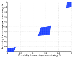
(a) $0.2$-equilibrium set.

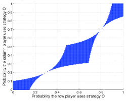
(b) $0.3$-equilibrium set.

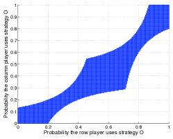
(c) $0.4$-equilibrium set.

Figure 4: Approximate equilibrium sets in BoS are contained in disjoint neighborhoods of equilibria for small $\epsilon$.

It was established in Lemma 6.3 that the potential function of a nearby potential game (with MPD $\delta$ to the original game), evaluated at the empirical frequency distribution, increases when this distribution is outside the $M\delta$-equilibrium set of the original game (where $M$ is the number of players). If $\delta$ is sufficiently small, then the $M\delta$-equilibria of the game will be contained in a small neighborhood of the equilibria, as illustrated above and shown in Lemma 6.2 (ii). Thus, for sufficiently small $\delta$, it is possible to establish that the potential of a close potential game increases outside a small neighborhood of the equilibria of the game. In Theorem 6.2, we use this observation to show that for sufficiently small $\delta$ the empirical frequencies of fictitious play dynamics converge to a neighborhood of an equilibrium. We state the theorem under the assumption that the original game has finitely many equilibria. This assumption generically holds, i.e., for any game a (nondegenerate) random perturbation of payoffs will lead to such a game with probability one (see Fudenberg and Tirole (1991)). When stating our result, we make use of the Lipschitz continuity of the mixed extension of the potential function, as established in Lemma 6.1.

Theorem 6.2.

Consider a game $\cal G$ and let $\hat{\cal G}$ be a close potential game such that $d({\cal G},\hat{\cal G})\leq\delta$. Denote the potential function of $\hat{\cal G}$ by $\phi$, and the Lipschitz constant of the mixed extension of $\phi$ by $L$. Assume that $\cal G$ has finitely many equilibria, and in $\cal G$ players update their strategies according to discrete-time fictitious play dynamics.

There exists some $\bar{\delta}>0$, and $\bar{\epsilon}>0$ (which are functions of utilities of $\cal G$ but not $\delta$) such that if $\delta<\bar{\delta}$, then the empirical frequencies of fictitious play converge to

$$\left\{\mathbf{x}\left|~{}||\mathbf{x}-\mathbf{x}_{k}||\leq\frac{4f(M\delta)ML}{\epsilon}+f(M\delta+\epsilon),\mbox{ for some equilibrium $\mathbf{x}_{k}$}\right.\right\},$$ (16)

for any $\epsilon$ such that $\bar{\epsilon}\geq\epsilon>0$, where $f:\mathbb{R}_{+}\rightarrow\mathbb{R}_{+}$ is an upper semicontinuous function satisfying $f(x)\rightarrow 0$ as $x\rightarrow 0$.

The proof of this theorem can be found in the Appendix, and it has three main steps illustrated in Figures 5 and 6. As explained earlier, for small $\delta$ and $\epsilon$, the $M\delta+\epsilon$-equilibrium set of the game is contained in disjoint neighborhoods of the equilibria of the game. Lemma 6.3 implies that potential evaluated at $\mu_{t}$ increases outside this approximate equilibrium set with strategy updates. In the proof, we first quantify the increase in the potential, when $\mu_{t}$ leaves this approximate equilibrium set and returns back to it at a later time instant (see Figure 5a). Then, using this increase condition we show that for sufficiently large $t$, $\mu_{t}$ can visit the approximate equilibrium set infinitely often only around one equilibrium, say $\mathbf{x}_{k^{\prime}}$ (see Figure 5b). This holds since, the increase condition guarantees that the potential increases significantly when $\mu_{t}$ leaves the neighborhood of an equilibrium $\mathbf{x}_{k}$, and reaches to that of $\mathbf{x}_{k^{\prime}}$. Finally, using the increase condition one more time, we establish that if after time $T$, $\mu_{t}$ visits the approximate equilibrium set only in the neighborhood of $\mathbf{x}_{k^{\prime}}$, we can construct a neighborhood of $\mathbf{x}_{k^{\prime}}$, which contains $\mu_{t}$ for all $t>T$ (see Figure 6). This neighborhood is expressed in (16).

(a) If empirical frequencies leave an approximate equilibrium set at time $t$, and return back to it at $t^{\prime}$, then $\phi(\mu_{t^{\prime}})>\phi(\mu_{t})$.

(b) For sufficiently large $t$, $\mu_{t}$ visits the component of the approximate equilibrium set contained in the neighborhood of a single equilibrium.

Figure 5: For small $\delta$ and $\epsilon$, $M\delta+\epsilon$-equilibrium set (enclosed by solid lines around equilibria $\mathbf{x}_{k^{\prime}}$ and $\mathbf{x}_{k}$) is contained in disjoint neighborhoods of equilibria. If the empirical frequency distribution, $\mu_{t}$, is outside this approximate equilibrium set, then the potential increases with each strategy update. Assume that empirical frequency distribution leaves an approximate equilibrium set (at time $t$) and returns back to it at a later time instant ($t^{\prime}>t$). We first quantify the resulting increase in the potential (left). If $\mu_{t}$ travels from the component of the approximate equilibrium set in the neighborhood of equilibrium $\mathbf{x}_{k}$ to that in the neighborhood of equilibrium $\mathbf{x}_{k^{\prime}}$, then the increase in the potential is significant, and consequently $\mu_{t}$ cannot visit the approximate equilibrium set in the neighborhood of equilibrium $\mathbf{x}_{k}$ at a later time instant (right).

Figure 6: If after time $T$, $\mu_{t}$ only visits the approximate equilibrium set in the neighborhood of a single equilibrium $\mathbf{x}_{k^{\prime}}$, then we can establish that $\mu_{t}$ never leaves a neighborhood of this equilibrium for $t>T$. The size of this neighborhood is denoted by $r$ in the figure and can be expressed as in Theorem 6.2.

Observe that if $\delta=0$, i.e., the original game is a potential game, then $f(M\delta)=0$, and Theorem 6.2 implies that empirical frequencies of fictitious play converge to the $f(\epsilon)$-neighborhood of equilibria for any $\epsilon$ such that $\bar{\epsilon}\geq\epsilon>0$. Thus, choosing $\epsilon$ arbitrarily small, and observing that $\lim_{x\rightarrow 0}f(x)=0$, our result implies that in potential games, empirical frequencies converge to the set of Nash equilibria. Hence, as a special case of Theorem 6.2, we obtain the convergence result of Monderer and Shapley (1996a).

Assume that $\delta\neq 0$ and a small $\epsilon<\bar{\epsilon}$ is given. If $\delta$ is sufficiently small then $f(M\delta)/\epsilon\approx 0$, since $\lim_{x\rightarrow 0}f(x)=0$. Consequently, $\frac{4f(M\delta)ML}{\epsilon}+f(M\delta+\epsilon)$ is small, and Theorem 6.2 establishes convergence of empirical frequencies to a small neighborhood of equilibria. Thus, we conclude that for games that are close to potential games, i.e., for $\delta\ll 1$, Theorem 6.2 establishes convergence of empirical frequencies to a small neighborhood of equilibria.

7 Conclusions

In this paper, we present a framework for studying the limiting behavior of adaptive learning dynamics in finite strategic form games by exploiting their relation to nearby potential games. We restrict our attention to better/best response, logit response and fictitious play dynamics. We show that for near-potential games trajectories of better/best response dynamics converge to $\epsilon$-equilibrium sets, where $\epsilon$ depends on closeness to a potential game. We study the stochastically stable strategy profiles of logit response dynamics and prove that they are contained in the set of strategy profiles that approximately maximize the potential function of a nearby potential game. In the case of fictitious play we focus on the empirical frequencies of players’ actions, and establish that they converge to a small neighborhood of equilibria in near-potential games. Our results suggest that games that are close to a potential game inherit the dynamical properties (such as convergence to approximate equilibrium sets) of potential games. Additionally, since a close potential game to a given game can be found by solving a convex optimization problem, as discussed in Section 3, this enables us to study dynamical properties of strategic form games by first identifying a nearby potential game to this game, and then studying the dynamical properties of the nearby potential game.

The framework presented in this paper opens up a number of interesting research directions. Among them, we mention the following:

Heterogeneous update rules:

In this paper we only analyzed the update rules in which players update their strategies using the same mechanism. For instance, we assumed that all players adopt best response, or logit response dynamics with the same parameter. The limiting behavior of dynamic processes, where players adhere to different update rules is still an open question, even for potential games. An interesting future research question is whether the techniques in this paper can be used to understand the limiting behavior of such update rules. For example, consider a potential game where all players update their strategies using logit response with different but “close” $\tau$ parameters. Can the outcome of this dynamic process be approximated with the outcome of logit response in a close potential game where all players use the same parameter for their updates?

Guaranteeing desirable limiting behavior:

Another promising research direction is to use our understanding of simple update rules, such as better/best response and logit response dynamics to design mechanisms that guarantee desirable limiting behavior, such as low efficiency loss and “fair” outcomes. It is well known that equilibria in games can be very different in terms of such properties (Roughgarden 2005). Hence, it is of interest to develop update rules that converge to a particular equilibrium, thus providing equilibrium refinement in the limit, or to find mechanisms that modify the underlying game in a way that can induce desirable limiting behavior. It has been shown in some cases that simple pricing mechanisms can ensure convergence to desirable equilibria in near-potential games (Candogan et al. 2010a). It is an interesting research direction to extend such mechanisms to general games.

Dynamics in “near” zero-sum and supermodular games:

Dynamical properties of simple update rules in zero-sum games and supermodular games are also well understood (Shamma and Arslan 2004, Milgrom and Roberts 1990). If a game is close to a zero-sum game or a supermodular game, does it still inherit some of the dynamical properties of the original game? If such “continuity” properties do not hold, then the results on dynamical properties of these classes of games may be fragile. Hence, it would be interesting to investigate whether analogous results to the ones in this paper can be established for these classes of games.

Appendix A Proofs of Section 6

Proof of Lemma 6.1:

(i) The mixed extension of $\nu$ can be given as in (8):

$$\nu(\mathbf{x})=\sum_{{\bf p}\in E}\nu({\bf p})\prod_{k\in{\cal M}}x^{k}({{p}^{k}}).$$

Hence $\nu(\mathbf{x})$ is equal to the sum of Lipschitz continuous functions $\{\nu({\bf p})\prod_{k\in{\cal M}}x^{k}({{p}^{k}})\}_{\mathbf{p}\in E}$. The claim follows since, as a function of $\mathbf{x}\in\prod_{m\in{\cal M}}\Delta E^{m}$, the Lipschitz constant of
$\nu({\bf p})\prod_{k\in{\cal M}}x^{k}({{p}^{k}})$ is bounded by $\nu({\bf p})\sqrt{M}\leq\nu({\bf p}){M}$.

(ii) Let $\nu:\prod_{m\in{\cal M}}\Delta E^{m}\rightarrow\mathbb{R}$ be a function such that

$$\nu(\mathbf{x})=-\max_{m\in{\cal M},p^{m}\in E^{m}}\left(u^{m}(p^{m},\mathbf{x}^{-m})-u^{m}(x^{m},\mathbf{x}^{-m})\right).$$ (17)

It follows from the definition of $\epsilon$-equilibrium that a strategy profile $\mathbf{x}$ is an $\epsilon$-equilibrium if and only if $\nu(\mathbf{x})\geq-\epsilon$.

By (i), it follows that mixed extensions of utility functions are Lipschitz continuous. Thus, the difference $u^{m}(p^{m},\mathbf{x}^{-m})-u^{m}(x^{m},\mathbf{x}^{-m})$ is Lipschitz continuous in $\mathbf{x}$. Since $\nu$ is obtained from maximum of finitely many such functions, we conclude that it is Lipschitz continuous with some constant $L$. It follows that if $||\mathbf{x}-\mathbf{y}||<\theta$, then $|\nu(\mathbf{x})-\nu(\mathbf{y})|<L\theta$. Thus, choosing $\theta<\gamma/L$, and recalling that $\mathbf{x}$ is an $\epsilon$-equilibrium if and only if $\nu(\mathbf{x})\geq-\epsilon$, the claim follows. ∎

Proof of Lemma 6.2:

(i) Consider the graph of $g$, i.e., $S=\{(v,\mathbf{x})|v\in\mathbb{R},\mathbf{x}\in g(v)\}$. The definition of $g$ suggests that $S$ can alternatively be written as

$$S=\left\{\left.(v,\mathbf{x})\in\mathbb{R}\times\prod_{m\in{\cal M}}\Delta E^{m}\right|\nu(\mathbf{x})\geq-v\right\}$$ (18)

Since $\nu$ is upper semicontinuous, the function $h:\mathbb{R}\times\prod_{m\in{\cal M}}\Delta E^{m}$, such that $h(v,\mathbf{x})=\nu(\mathbf{x})+v$, is also an upper semicontinuous function. Since upper level sets of upper semicontinuous functions are closed (see Berge (1963)), the set $\left\{(v,\mathbf{x})\in\mathbb{R}\times\prod_{m\in{\cal M}}\Delta E^{m}|h(v,\mathbf{x})\geq 0\right\}$, or equivalently $S$ is a closed subset of $\mathbb{R}\times\prod_{m\in{\cal M}}\Delta E^{m}$. Thus, the graph of $g$ is closed, and since $\prod_{m\in{\cal M}}\Delta E^{m}$ is a compact set the claim follows from Definition 6.2.

(ii) Let $\nu:\prod_{m\in{\cal M}}\Delta E^{m}\rightarrow\mathbb{R}$ be as in (17). i.e.,

$$\nu(\mathbf{x})=-\max_{m\in{\cal M},p^{m}\in E^{m}}\left(u^{m}(p^{m},\mathbf{x}^{-m})-u^{m}(x^{m},\mathbf{x}^{-m})\right).$$

As explained in the proof of Lemma 6.1, $\mathbf{x}$ is an $\epsilon$-equilibrium if and only if $\nu(\mathbf{x})\geq-\epsilon$. The claim follows from part (i) by noting that $\nu$ is a continuous function, and $g(\alpha)={\cal X}_{\alpha}=\{\mathbf{x|\nu(\mathbf{x})\geq-\alpha}\}$. ∎

Proof of Corollary 6.1:

Let $\epsilon_{n}=M\delta+\frac{1}{n}$ for $n\in\mathrm{Z}_{+}$. Observe that since the mixed extension of the potential function is continuous, $C$ and $C_{\epsilon_{n}}$ are closed sets for any $n\in\mathrm{Z}_{+}$. Since $C$ is closed $\min_{\mathbf{y}\in C}||\mathbf{x}-\mathbf{y}||$ is well-defined for any $\mathbf{x}\in\prod_{m\in{\cal M}}\Delta E^{m}$.

We claim that for any $\theta>0$ the set

$$S_{\theta}=\left\{\mathbf{x}\in\prod_{m\in{\cal M}}\Delta E^{m}\left|\min_{\mathbf{y}\in C}||\mathbf{x}-\mathbf{y}||<\theta\right.\right\},$$ (19)

is such that $C_{\epsilon_{n}}\subset S_{\theta}$ for some $n$. Note that if this claim holds, then it follows from Theorem 6.1 that there exists some $T_{\theta}$ such that for all $t>T_{\theta}$ we have $\mu_{t}\in S_{\theta}$. Using the definition of $S_{\theta}$ given in (19), this implies

$$\limsup_{t\rightarrow\infty}~{}\min_{\mathbf{x}\in C}||\mathbf{x}-\mu_{t}||<\theta.$$ (20)

Moreover, since $\theta>0$ is arbitrary, and $||\mathbf{x}-\mu_{t}||\geq 0$, using (20) we obtain

$$\lim_{t\rightarrow\infty}~{}\min_{\mathbf{x}\in C}||\mathbf{x}-\mu_{t}||=0.$$

Thus, if we prove $C_{\epsilon_{n}}\subset S_{\theta}$ for some $n$, it follows that $\mu_{t}$ converges to $C$.

In order to prove $C_{\epsilon_{n}}\subset S_{\theta}$ we first obtain a certificate which can be used to guarantee that a mixed strategy profile belongs to $S_{\theta}$. Then, we show that for large enough $n$ any $\mathbf{z}\in C_{\epsilon_{n}}$ satisfies this certificate, and hence belongs to $S_{\theta}$.

It follows from Lemma 6.2 (i) (by setting $\nu=\phi$ and $v=-\min_{\mathbf{y}\in{\cal X}_{M\delta}}\phi(\mathbf{y})$) and definition of upper semicontinuity (Definition 6.2) that there exists $\gamma>0$ such that $\theta$ neighborhood of $\{\mathbf{x}|\phi(\mathbf{x})\geq\min_{\mathbf{y}\in{\cal X}_{M\delta}}\phi(\mathbf{y})\}$ contains $\{\mathbf{x}|\phi(\mathbf{x})\geq\min_{\mathbf{y}\in{\cal X}_{M\delta}}\phi(\mathbf{y})-\gamma\}$. Hence, for any $\mathbf{z}$ satisfying $\phi(\mathbf{z})\geq\min_{\mathbf{y}\in{\cal X}_{M\delta}}\phi(\mathbf{y})-\gamma$ there exists some $\mathbf{x}$ satisfying $\phi(\mathbf{x})\geq\min_{\mathbf{y}\in{\cal X}_{M\delta}}\phi(\mathbf{y})$ and $||\mathbf{x}-\mathbf{z}||<\theta$. Note that the definition of $S_{\theta}$ implies that $\mathbf{z}$ for which there exists such $\mathbf{x}$ belongs to $S_{\theta}$. Thus, if $\phi(\mathbf{z})\geq\min_{\mathbf{y}\in{\cal X}_{M\delta}}\phi(\mathbf{y})-\gamma$ it follows that $\mathbf{z}\in S_{\theta}$.

We next show that for large enough $n$, any $\mathbf{z}$ which belongs to $C_{\epsilon_{n}}$, satisfies the above certificate and hence belongs to $S_{\theta}$. Let $L$ denote the Lipschitz constant for the mixed extension of $\phi$, as given in Lemma 6.1 (i), and define $\theta^{\prime}=\gamma/L>0$. Lemma 6.2 (ii) and Definition 6.2 imply that for large enough $n$, ${\cal X}_{M\delta+\frac{1}{n}}$ is contained in $\theta^{\prime}$ neighborhood of ${\cal X}_{M\delta}$, i.e., if $\mathbf{y}\in{\cal X}_{M\delta+\frac{1}{n}}$ then there exists $\mathbf{x}\in{\cal X}_{M\delta}$ such that $||\mathbf{x}-\mathbf{y}||<\theta^{\prime}$. Moreover, by Lemma 6.1 (i), it follows that $\phi(\mathbf{y})\geq\phi(\mathbf{x})-L\theta^{\prime}=\phi(\mathbf{x})-\gamma$. Thus, we conclude that there exists large enough $n$ such that

$$\min_{\mathbf{y}\in{\cal X}_{M\delta+1/n}}\phi(\mathbf{y})\geq\min_{\mathbf{y}\in{\cal X}_{M\delta}}\phi(\mathbf{y})-\gamma.$$ (21)

Let $\mathbf{z}\in C_{\epsilon_{n}}$ for some $n$ for which (21) holds. By definition of $C_{\epsilon}$ it follows that $\phi(\mathbf{z})\geq\min_{\mathbf{y}\in{\cal X}_{M\delta+1/n}}\phi(\mathbf{y})$. Thus, (21) implies that $\phi(\mathbf{z})\geq\min_{\mathbf{y}\in{\cal X}_{M\delta}}\phi(\mathbf{y})-\gamma$. However, as argued before such $\mathbf{z}$ belong to $S_{\theta}$. Hence, we have established that for large enough $n$, if $\mathbf{z}\in C_{\epsilon_{n}}$ then $\mathbf{z}\in S_{\theta}$. Therefore, the claim follows. ∎

Proof of Theorem 6.2:

Assume that $\cal G$ has $l$ equilibria, denoted by $\mathbf{x}_{1},\dots,\mathbf{x}_{l}$. Define the minimum pairwise distance between the equilibria as $d\triangleq\min_{i\neq j}||\mathbf{x}_{i}-\mathbf{x}_{j}||$. Let $f:\mathbb{R}_{+}\rightarrow\mathbb{R}_{+}$ be a function such that

$$f(\alpha)=\max_{\mathbf{x}\in{\cal X}_{\alpha}}\min_{k\in\{1,\dots,l\}}||\mathbf{x}-\mathbf{x}_{k}||,$$ (22)

for all $\alpha\in\mathbb{R}_{+}$. Note that $\min_{k\in\{1,\dots,l\}}||\mathbf{x}-\mathbf{x}_{k}||$ is continuous in $\mathbf{x}$, since it is minimum of finitely many continuous functions. Moreover, ${\cal X}_{\alpha}$ is a compact set, since $\epsilon$-equilibria are defined by finitely many inequality constraints of the form (9). Therefore, in (22) maximum is achieved and $f$ is well-defined for all $\alpha\geq 0$. From the definition of $f$, it follows that the union of closed balls of radius $f(\alpha)$, centered at equilibria, contain $\alpha$-equilibrium set of the game. Thus, intuitively, $f(\alpha)$ captures the size of a closed neighborhood of equilibria, which contains $\alpha$-equilibria of the underlying game. This is illustrated in Figure 7.

Figure 7: Consider a game with a unique equilibrium $\mathbf{x}_{k}$. The $\alpha$-equilibrium set of the game (enclosed by a solid line around $\mathbf{x}_{k}$) is contained in the $f(\alpha)$ neighborhood of this equilibrium.

Let $a>0$ be such that $f(a)<d/4$, i.e., every $a$-equilibrium is at most $d/4$ distant from an equilibrium of a game. Lemma 6.2 (ii) implies (using upper semicontinuity at $\alpha=0$) that such $a$ exists. Since $d$ is defined as the minimum pairwise distance between the equilibria, it follows that $a$-equilibria of the game are contained in disjoint $f(a)<d/4$ neighborhoods around equilibria of the game, i.e., if $\mathbf{x}\in{\cal X}_{a}$, then $||\mathbf{x}-\mathbf{x}_{k}||\leq f(a)$ for exactly one equilibrium $\mathbf{x}_{k}$. Moreover, for $a_{1}\leq a$, since ${\cal X}_{a_{1}}\subset{\cal X}_{a}$, it follows that $a_{1}$-equilibria of the game are contained in disjoint neighborhoods of equilibria.

We prove the theorem in 5 steps summarized below. First two steps explore the properties of function $f$, and define $\bar{\delta}$ and $\bar{\epsilon}$ presented in the theorem statement. Last three steps are the main steps of the proof, where we establish convergence of fictitious play to a neighborhood of equilibria.

• Step 1: We first show that $f$ is (i) weakly increasing, (ii) upper semicontinuous, and it satisfies (iii) $f(0)=0$, (iv) $f(x)\rightarrow 0$ as $x\rightarrow 0$.

• Step 2: We show that there exists some $\bar{\delta}>0$ and $\bar{\epsilon}>0$ such that the following inequalities hold:

  $$M\bar{\delta}+\bar{\epsilon}<a,$$ (23)

  and

  $$f(M\bar{\delta}+\bar{\epsilon})<\frac{(a-M\bar{\delta})d}{24LM}.$$ (24)

  We will prove the statement of the theorem assuming that $0\leq\delta<\bar{\delta}$, and establish convergence to the set in (16), for any $\epsilon$ such that $0<\epsilon\leq\bar{\epsilon}$. As can be seen from the definition of $a$ and $f$ (see (22)), the first inequality guarantees that $M\bar{\delta}+\bar{\epsilon}$-equilibrium set is contained in disjoint neighborhoods of equilibria, and the second one guarantees that these neighborhoods are small. In Step 4, we will exploit this observation, and use the inequalities in (23) and (24) to establish that the empirical frequency distribution $\mu_{t}$ can visit the component of ${\cal X}_{M\delta+\bar{\epsilon}}$ contained in the neighborhood of only a single equilibrium infinitely often.

• Step 3: Let $\epsilon_{1},\epsilon_{2}$ be such that $\epsilon_{2}>\epsilon_{1}>0$. Assume that (i) at some time instant $T$, $\mu_{t}$ is contained in ${\cal X}_{M\delta+\epsilon_{1}}$, (ii) at time instants $T_{1}$ and $T_{2}$ (such that $T_{2}>T_{1}>T$) $\mu_{t}$ leaves ${\cal X}_{M\delta+\epsilon_{1}}$ and ${\cal X}_{M\delta+\epsilon_{2}}$ respectively and (iii) at time instants $T_{2}^{\prime}$ and $T_{1}^{\prime}$ (such that $T_{1}^{\prime}>T_{2}^{\prime}>T_{2}$) $\mu_{t}$ returns back to ${\cal X}_{M\delta+\epsilon_{2}}$ and ${\cal X}_{M\delta+\epsilon_{1}}$ respectively. In Figure 8, the path $\mu_{t}$ follows between $T_{1}$ and $T_{1}^{\prime}$ is illustrated.

  In this step, we provide a lower bound on $\phi(\mu_{T_{1}^{\prime}})-\phi(\mu_{T_{1}})$, i.e., the increase in the potential when $\mu_{t}$ follows such a path. This lower bound holds for any $\epsilon_{1}$ and $\epsilon_{2}$ provided that $\epsilon_{2}>\epsilon_{1}>0$. We use this result by choosing different values for $\epsilon_{1}$ and $\epsilon_{2}$ in Steps 4 and 5.

  Our lower bound in Step 3 is a function of ${\epsilon_{2}}$. In addition to this lower bound, in Steps 4 and 5, we use the ${M\delta+\epsilon_{1}}$ equilibrium set and Lipschitz continuity of the potential to provide an upper bound on $\phi(\mu_{T_{1}^{\prime}})-\phi(\mu_{T_{1}})$ as a function of $\epsilon_{1}$. Thus, properties of ${M\delta+\epsilon_{1}}$ and ${M\delta+\epsilon_{2}}$ equilibrium sets are exploited for obtaining upper and lower bounds on $\phi(\mu_{T_{1}^{\prime}})-\phi(\mu_{T_{1}})$ respectively. We establish convergence of fictitious play updates to a neighborhood of an equilibrium by using these bounds together in Steps 4 and 5. We emphasize that allowing for two different approximate equilibrium sets leads to better bounds on $\phi(\mu_{T_{1}^{\prime}})-\phi(\mu_{T_{1}})$, and a more informative characterization of the limiting behavior of fictitious play, as opposed to using a single approximate equilibrium set, i.e., setting $\epsilon_{1}=\epsilon_{2}$.

• Step 4: Our objective in this step is to establish that fictitious play can visit the component of an approximate equilibrium set contained in the neighborhood of only one equilibrium infinitely often.

  Let $\epsilon_{1}=\bar{\epsilon}$ and $\epsilon_{2}=a-M\bar{\delta}$. By (23) we have $\epsilon_{1}<\epsilon_{2}$, and using the definition of $a$ we establish that ${\cal X}_{M\delta+\epsilon_{1}}$ and ${\cal X}_{M\delta+\epsilon_{2}}$ are contained in disjoint neighborhoods of equilibria. Assume that $\mu_{t}$ leaves the components of ${\cal X}_{M\delta+\epsilon_{1}}$ and ${\cal X}_{M\delta+\epsilon_{2}}$ in the neighborhood of equilibrium $\mathbf{x}_{k}$, and reaches to a similar neighborhood around equilibrium $\mathbf{x}_{k^{\prime}}$. Using Step 3 we establish a lower bound on the increase in the potential when $\mu_{t}$ follows such a trajectory. We also provide an upper bound, using the Lipschitz continuity of the potential and inequalities (23) and (24). Comparing these bounds, we establish that the maximum potential in the neighborhood of equilibrium $\mathbf{x}_{k}$ is lower than the minimum potential in the neighborhood of $\mathbf{x}_{k^{\prime}}$. Since, $\mathbf{x}_{k}$ and $\mathbf{x}_{k^{\prime}}$ are arbitrary, this observation implies that $\mu_{t}$ cannot visit the component of ${\cal X}_{M\delta+\epsilon_{1}}$ contained in the neighborhood of $\mathbf{x}_{k}$ at a later time instant. Hence, it follows that $\mu_{t}$ visits only one such component infinitely often.

• Step 5: In this step we show that $\mu_{t}$ converges to the approximate equilibrium set given in the theorem statement.

  Let $\epsilon_{1},\epsilon_{2}$ be such that $0<\epsilon_{1}<\epsilon_{2}\leq\bar{\epsilon}$. We consider the equilibrium, whose neighborhood is visited infinitely often (as obtained in Step 4), and a trajectory of $\mu_{t}$ which leaves the components of ${\cal X}_{M\delta+\epsilon_{1}}$ and ${\cal X}_{M\delta+\epsilon_{2}}$ contained in the neighborhood of this equilibrium and returns back to these sets at a later time instant (as illustrated in Figure 8). As in Step 4, Lipschitz continuity of $\phi$ is used to obtain an upper bound on the increase in the potential between the end points of this trajectory. Together with the lower bound obtained in Step 3, this provides a bound on how far $\mu_{t}$ can get from the component of ${\cal X}_{M\delta+\epsilon_{2}}$ contained in this neighborhood. Choosing $\epsilon_{1}$ arbitrarily small (for a fixed $\epsilon_{2}$) we obtain the tightest such bound. Using this result, we quantify how far $\mu_{t}$ can get from the equilibria of the game (after sufficient time) and the theorem follows.

Next we prove each of these steps.

Step 1:

By definition ${\cal X}_{\alpha_{1}}\subset{\cal X}_{\alpha}$ for any $\alpha_{1}\leq\alpha$. Since the feasible set of the maximization problem in (22) is given by ${\cal X}_{\alpha}$, this implies that $f(\alpha_{1})\leq f(\alpha)$, i.e., $f$ is a weakly increasing function of its argument. Note that the feasible set of the maximization problem in (22) can be given by the correspondence $g(\alpha)={\cal X}_{\alpha}$, which is upper semi continuous in $\alpha$ as shown in Lemma 6.2 (ii). Since as a function of $\mathbf{x}$, $\min_{k\in\{1,\dots,l\}}||\mathbf{x}-\mathbf{x}_{k}||$ is continuous it follows from Berge’s maximum theorem (see Berge (1963)) that for $\alpha\geq 0$, $f(\alpha)$ is an upper semicontinuous function.

The set ${\cal X}_{0}$ corresponds to the set of equilibria of the game, hence ${\cal X}_{0}=\{\mathbf{x}_{1},\dots,\mathbf{x}_{l}\}$. Thus, the definition of $f$ implies that $f(0)=0$. Moreover, upper semicontinuity of $f$ implies that for any $\epsilon>0$, there exists some neighborhood $V$ of $0$, such that $f(x)\leq\epsilon$ for all $x\in V$. Since, $f(x)\geq 0$ by definition, this implies that $\lim_{x\rightarrow 0}f(x)$ exists and equals to $0$.

Step 2:

Let $\bar{\delta}>0$ be small enough such that $M\bar{\delta}<a/2$. Since $\lim_{x\rightarrow 0}f(x)=0$, it follows that for sufficiently small $\bar{\delta}$ and $\bar{\epsilon}$, we obtain $f(M\bar{\delta}+\bar{\epsilon})<\frac{ad}{48LM}<\frac{(a-M\bar{\delta})d}{24LM}$ and $M\bar{\delta}+\bar{\epsilon}<a$.

Step 3:

Let $\epsilon_{1},\epsilon_{2}$ be such that $0<\epsilon_{1}<\epsilon_{2}$. Assume $T>0$ is large enough so that for $t>T$,

$$\phi(\mu_{t+1})-\phi(\mu_{t})\geq\frac{2\epsilon_{1}}{3(t+1)} \mu_{t}\notin{\cal X}_{M\delta+\epsilon_{1}}$$ if , and similarly (25)

$$\phi(\mu_{t+1})-\phi(\mu_{t})\geq\frac{2\epsilon_{2}}{3(t+1)} \mu_{t}\notin{\cal X}_{M\delta+\epsilon_{2}}$$ if .

Existence of $T$ satisfying these inequalities follows from Lemma 6.3, since for large $T$ and $t>T$, this lemma implies $\phi(\mu_{t+1})-\phi(\mu_{t})\geq\frac{\epsilon_{1}}{(t+1)}+O\left(\frac{1}{t^{2}}\right)\geq\frac{2\epsilon_{1}}{3(t+1)}$ if $\mu_{t}\notin{\cal X}_{M\delta+\epsilon_{1}}$, and similarly if $\mu_{t}\notin{\cal X}_{M\delta+\epsilon_{2}}$.

Since $\phi(\mu_{t})$ increases outside $M\delta+\epsilon_{1}$-equilibrium set for $t>T$, as (25) suggests, it follows that $\mu_{t}$ visits ${\cal X}_{M\delta+\epsilon_{1}}$ (and ${\cal X}_{M\delta+\epsilon_{2}}$ since ${\cal X}_{M\delta+\epsilon_{1}}\subset{\cal X}_{M\delta+\epsilon_{2}}$) infinitely often. Otherwise $\phi(\mu_{t})$ increases unboundedly, and we reach a contradiction since mixed extension of the potential is a bounded function.

Assume that at some time after $T$, $\mu_{t}$ leaves ${\cal X}_{M\delta+\epsilon_{1}}$ and ${\cal X}_{M\delta+\epsilon_{2}}$ and returns back to ${\cal X}_{M\delta+\epsilon_{1}}$ at a later time instant. In this step, we quantify how much the potential increases when $\mu_{t}$ follows such a path. We first define time instants $T_{1}$, $T_{2}$, $T_{1}^{\prime}$, and $T_{2}^{\prime}$ satisfying $T<T_{1}\leq T_{2}<T_{2}^{\prime}\leq T_{1}^{\prime}$, as follows:

• $T_{1}$ is a time instant when $\mu_{t}$ leaves ${\cal X}_{M\delta+\epsilon_{1}}$, i.e., $\mu_{T_{1}-1}\in{\cal X}_{M\delta+\epsilon_{1}}$ and $\mu_{t}\notin{\cal X}_{M\delta+\epsilon_{1}}$ for $T_{1}\leq t<T_{1}^{\prime}$.

• $T_{2}$ is a time instant when $\mu_{t}$ leaves ${\cal X}_{M\delta+\epsilon_{2}}$, i.e., $\mu_{T_{2}-1}\in{\cal X}_{M\delta+\epsilon_{2}}$ and $\mu_{t}\notin{\cal X}_{M\delta+\epsilon_{2}}$ for $T_{2}\leq t<T_{2}^{\prime}$.

• $T_{2}^{\prime}$ is the first time instant after $T_{2}$ when $\mu_{t}$ returns back to ${\cal X}_{M\delta+\epsilon_{2}}$, i.e., $\mu_{T_{2}^{\prime}-1}\notin{\cal X}_{M\delta+\epsilon_{2}}$ and $\mu_{T_{2}^{\prime}}\in{\cal X}_{M\delta+\epsilon_{2}}$.

• $T_{1}^{\prime}$ is the first time instant after $T_{1}$ when $\mu_{t}$ returns back to ${\cal X}_{M\delta+\epsilon_{1}}$, i.e., $\mu_{T_{1}^{\prime}-1}\notin{\cal X}_{M\delta+\epsilon_{1}}$ and $\mu_{T_{1}^{\prime}}\in{\cal X}_{M\delta+\epsilon_{1}}$.

The definitions are illustrated in Figure 8. We next provide a lower bound on the quantity $\phi(\mu_{T_{1}^{\prime}})-\phi(\mu_{T_{1}})$. Note that if there are multiple time instants between $T_{1}$ and $T_{1}^{\prime}$ for which $\mu_{t}$ leaves ${\cal X}_{M\delta+\epsilon_{2}}$ (as in the figure), any of these time instants can be chosen as $T_{2}$ to obtain a lower bound.

Figure 8: Trajectory of $\mu_{t}$ (initialized at the left end of the dashed line) is illustrated. $T_{1}$ and $T_{2}$ correspond to the time instants $\mu_{t}$ leaves ${\cal X}_{M\delta+\epsilon_{1}}$ and ${\cal X}_{M\delta+\epsilon_{2}}$ respectively. $T_{1}^{\prime}$ and $T_{2}^{\prime}$ correspond to the time instants $\mu_{t}$ enters ${\cal X}_{M\delta+\epsilon_{1}}$ and ${\cal X}_{M\delta+\epsilon_{2}}$ respectively.

By definition, for $t$ such that $T_{2}\leq t<T_{2}^{\prime}$, we have $\mu_{t}\notin{\cal X}_{M\delta+\epsilon_{2}}$, and for $t$ such that $T_{1}\leq t<T_{2}$ or $T_{2}^{\prime}\leq t<T_{1}^{\prime}$, we have $\mu_{t}\notin{\cal X}_{M\delta+\epsilon_{1}}$. Thus, it follows from (25) that

$$\phi(\mu_{t+1})-\phi(\mu_{t})\geq\frac{2\epsilon_{2}}{3(t+1)}\qquad\mbox{ for $T_{2}\leq t<T_{2}^{\prime}$},$$ (26)

and consequently,

$$\phi(\mu_{T_{2}^{\prime}})-\phi(\mu_{T_{2}})=\sum_{t=T_{2}}^{T_{2}^{\prime}-1}\phi(\mu_{t+1})-\phi(\mu_{t})\geq\sum_{t=T_{2}}^{T_{2}^{\prime}-1}\frac{2\epsilon_{2}}{3(t+1)}.$$ (27)

Similarly, since $\mu_{t}\notin{\cal X}_{M\delta+\epsilon_{1}}$ for $t$ such that $T_{1}\leq t<T_{2}$ or $T_{2}^{\prime}\leq t<T_{1}^{\prime}$, using (25) we establish

$$\phi(\mu_{T_{1}^{\prime}})-\phi(\mu_{T_{2}^{\prime}})=\sum_{t=T_{2}^{\prime}}^{T_{1}^{\prime}-1}\phi(\mu_{t+1})-\phi(\mu_{t})\geq\sum_{t=T_{2}^{\prime}}^{T_{1}^{\prime}-1}\frac{2\epsilon_{1}}{3(t+1)},$$ (28)

$$\phi(\mu_{T_{2}})-\phi(\mu_{T_{1}})=\sum_{t=T_{1}}^{T_{2}-1}\phi(\mu_{t+1})-\phi(\mu_{t})\geq\sum_{t=T_{1}}^{T_{2}-1}\frac{2\epsilon_{1}}{3(t+1)}.$$ (29)

Since $\phi(\mu_{T_{1}^{\prime}})-\phi(\mu_{T_{1}})=\left(\phi(\mu_{T_{1}^{\prime}})-\phi(\mu_{T_{2}^{\prime}})\right)+\left(\phi(\mu_{T_{2}^{\prime}})-\phi(\mu_{T_{2}})\right)+\left(\phi(\mu_{T_{2}})-\phi(\mu_{T_{1}})\right)$, it follows from (27), (28) and (29) that

$$\phi(\mu_{T_{1}^{\prime}})-\phi(\mu_{T_{1}})\geq\sum_{t=T_{2}}^{T_{2}^{\prime}-1}\frac{2\epsilon_{2}}{3(t+1)}.$$ (30)

Step 4:

Let $\epsilon_{2}=a-M\bar{\delta}$, and $\epsilon_{1}=\bar{\epsilon}$. By definition of $\bar{\epsilon}$ and $\bar{\delta}$ (see Step 2), it follows that $\epsilon_{2}>\epsilon_{1}>0$. Assume that $\delta<\bar{\delta}$. Since $a=M\bar{\delta}+{\epsilon_{2}}>M\delta+{\epsilon_{2}}>M\delta+{\epsilon_{1}}$ we obtain ${\cal X}_{M\delta+\epsilon_{1}}\subset{\cal X}_{M\delta+\epsilon_{2}}\subset{\cal X}_{a}$. By definition of $a$, ${\cal X}_{a}$ is contained in disjoint neighborhoods of equilibria. Thus, it follows that components of ${\cal X}_{M\delta+\epsilon_{1}}$ and ${\cal X}_{M\delta+\epsilon_{2}}$ are also contained in disjoint neighborhoods of equilibria. Hence, the definition of $f$ suggests that if $\mathbf{x}\in{\cal X}_{M\delta+\epsilon_{1}}$ then $||\mathbf{x}_{k}-\mathbf{x}||\leq f({M\delta+\epsilon_{1}})$ (similarly if $\mathbf{x}\in{\cal X}_{M\delta+\epsilon_{2}}$ , then $||\mathbf{x}_{k}-\mathbf{x}||\leq f({M\delta+\epsilon_{2}})$) for exactly one equilibrium $\mathbf{x}_{k}$.

Let $T_{1},T_{2},T_{1}^{\prime}$ and $T_{2}^{\prime}$ be defined as in Step 3. In this step, by obtaining an upper bound on $\phi(\mu_{T_{1}^{\prime}})-\phi(\mu_{T_{1}})$ and refining the lower bound obtained in Step 3 for given values of $\epsilon_{1}$ and $\epsilon_{2}$, we prove that after sufficient time $\mu_{t}$ can visit the component of ${\cal X}_{M\delta+\epsilon_{1}}$ in the neighborhood of a single equilibrium.

Assume that $\mu_{t}$ leaves the component of the ${M\delta+\epsilon_{1}}$-equilibrium set in the neighborhood of equilibrium $\mathbf{x}_{k}$, and it reaches to another component in the neighborhood of equilibrium $\mathbf{x}_{k^{\prime}}$. Since, by definition $\mu_{T_{1}-1},\mu_{T_{1}^{\prime}}\in{\cal X}_{M\delta+\epsilon_{1}}$, and $\mu_{T_{2}-1},\mu_{T_{2}^{\prime}}\in{\cal X}_{M\delta+\epsilon_{2}}$, it follows that $\mu_{T_{1}-1}$ and $\mu_{T_{2}-1}$ belong to neighborhoods of equilibrium $\mathbf{x}_{k}$, whereas, $\mu_{T_{1}^{\prime}}$ and $\mu_{T_{2}^{\prime}}$ belong to neighborhoods of $\mathbf{x}_{k^{\prime}}$, i.e.,

$$||\mathbf{x}_{k}-\mu_{T_{1}-1}||\leq f({M\delta+\epsilon_{1}})\qquad \mbox{and}\qquad||\mathbf{x}_{k}-\mu_{T_{2}-1}||\leq f({M\delta+\epsilon_{2}})\mbox{, whereas,}$$ (31)

$$||\mathbf{x}_{k^{\prime}}-\mu_{T_{1}^{\prime}}||\leq f({M\delta+\epsilon_{1}})\qquad \mbox{and}\qquad||\mathbf{x}_{k^{\prime}}-\mu_{T_{2}^{\prime}}||\leq f({M\delta+\epsilon_{2}}).$$ (32)

By definition of $d$ we have $||\mathbf{x}_{k}-\mathbf{x}_{k^{\prime}}||\geq d$. Since $a>M\delta+\epsilon_{2}$, it follows that $f(M\delta+\epsilon_{2})\leq f(a)<d/4$, and hence the second inequalities in (31) and (32) imply

$$||\mu_{T_{2}^{\prime}}-\mu_{T_{2}-1}||>\frac{d}{2}.$$ (33)

Using this inequality, we next refine the lower bound on $\phi(\mu_{T_{1}^{\prime}})-\phi(\mu_{T_{1}})$ obtained in Step 3. By (10), with an update at time $t$, the empirical frequency distribution can change by at most

$$||\mu_{t+1}-\mu_{t}||=\frac{1}{t+1}||\mu_{t}-I_{t}||\leq\frac{1}{t+1}(||\mu_{t}||+||I_{t}||)\leq\frac{2M}{t+1},$$ (34)

where the last inequality follows from the fact that $\mu_{t}=\{\mu_{t}^{m}\}_{m\in{\cal M}}$, and $I_{t}=\{I_{t}^{m}\}_{m\in{\cal M}}$, and $||\mu_{t}^{m}||,||I_{t}^{m}||\leq 1$, since $I_{t}^{m},\mu_{t}^{m}\in\Delta E^{m}$. Hence, if $T_{2}$ is sufficiently large, then $||\mu_{T_{2}}-\mu_{T_{2}-1}||$ is small enough so that (33) implies $||\mu_{T_{2}^{\prime}}-\mu_{T_{2}}||>\frac{d}{2}.$ Using this together with (34), we conclude

$$\sum_{t=T_{2}}^{T_{2}^{\prime}-1}\frac{2M}{t+1}\geq\sum_{t=T_{2}}^{T_{2}^{\prime}-1}||\mu_{t+1}-\mu_{t}||\geq||\sum_{t=T_{2}}^{T_{2}^{\prime}-1}\mu_{t+1}-\mu_{t}||=||\mu_{T_{2}^{\prime}}-\mu_{T_{2}}||>\frac{d}{2}.$$ (35)

Thus, the lower bound on $\phi(\mu_{T_{1}^{\prime}})-\phi(\mu_{T_{1}})$ provided in (30) takes the following form:

$$\phi(\mu_{T_{1}^{\prime}})-\phi(\mu_{T_{1}})\geq\sum_{t=T_{2}}^{T_{2}^{\prime}-1}\frac{2\epsilon_{2}}{3(t+1)}\geq\frac{\epsilon_{2}d}{6M}.$$ (36)

Next we provide an upper bound on $\phi(\mu_{T_{1}^{\prime}})-\phi(\mu_{T_{1}})$, using Lipschitz continuity of the potential and the properties of the $M\delta+\epsilon_{1}$ equilibrium set. Let $\overline{\phi}_{k}=\max_{\{\mathbf{x}~{}|~{}||\mathbf{x}-\mathbf{x}_{k}||\leq f(M\delta+\epsilon_{1})\}}\phi(\mathbf{x}),$ and define $\mathbf{y}_{k}$ as a strategy profile which achieves this maximum. Similarly, let $\underline{\phi}_{k^{\prime}}=\min_{\{\mathbf{x}~{}|~{}||\mathbf{x}-\mathbf{x}_{k^{\prime}}||\leq f(M\delta+\epsilon_{1})\}}\phi(\mathbf{x})$ and define $\mathbf{y}_{k^{\prime}}$ as a strategy profile which achieves this minimum. Observe that

$$\underline{\phi}_{k^{\prime}}-\overline{\phi}_{k} =\phi(\mathbf{y}_{k^{\prime}})-\phi(\mathbf{y}_{k})$$ (37)

$$=\left(\phi(\mathbf{y}_{k^{\prime}})-\phi(\mu_{T_{1}^{\prime}})\right)+\left(\phi(\mu_{T_{1}^{\prime}})-\phi(\mu_{T_{1}})\right)+\left(\phi(\mu_{T_{1}})-\phi(\mathbf{y}_{k})\right).$$

Note that by (31) and (32), and the definitions of $\mathbf{y}_{k}$ and $\mathbf{y}_{k^{\prime}}$, we have $\mu_{T_{1}^{\prime}},\mathbf{y}_{k^{\prime}}\in\{\mathbf{x}~{}|~{}||\mathbf{x}-\mathbf{x}_{k^{\prime}}||\leq f(M\delta+\epsilon_{1})\}$, and $\mu_{T_{1}-1},\mathbf{y}_{k}\in\{\mathbf{x}~{}|~{}||\mathbf{x}-\mathbf{x}_{k}||\leq f(M\delta+\epsilon_{1})\}$. Hence, using Lipschitz continuity of $\phi$ (and denoting the Lipschitz constant by $L$) it follows that $\phi(\mathbf{y}_{k^{\prime}})-\phi(\mu_{T_{1}^{\prime}})\geq-2Lf(M\delta+\epsilon_{1})$, and $\phi(\mu_{T_{1}-1})-\phi(\mathbf{y}_{k})\geq-2Lf(M\delta+\epsilon_{1})$. Moreover, (34) and Lipschitz continuity of $\phi$ imply that $\phi(\mu_{T_{1}})-\phi(\mu_{T_{1}-1})=O\left(\frac{1}{T_{1}}\right)$. Thus, using (37) we obtain the following upper bound on $\phi(\mu_{T_{1}^{\prime}})-\phi(\mu_{T_{1}})$:

$$\underline{\phi}_{k^{\prime}}-\overline{\phi}_{k}+4Lf(M\delta+\epsilon_{1})+O\left(\frac{1}{T_{1}}\right)\geq\phi(\mu_{T_{1}^{\prime}})-\phi(\mu_{T_{1}}).$$ (38)

Using the lower and upper bounds we obtained in (36) and (38), it follows that

$$\underline{\phi}_{k^{\prime}}-\overline{\phi}_{k}+4Lf(M\delta+\epsilon_{1})+O\left(\frac{1}{T_{1}}\right)\geq\frac{\epsilon_{2}d}{6M}.$$ (39)

Since $\epsilon_{2}=a-M\bar{\delta}$, and $\epsilon_{1}=\bar{\epsilon}$, using the fact that $f$ is an increasing function and $\delta<\bar{\delta}$, it follows from (39) that

$$\underline{\phi}_{k^{\prime}}-\overline{\phi}_{k}\geq\frac{(a-M\bar{\delta})d}{6M}-4Lf(M\delta+\bar{\epsilon})+O\left(\frac{1}{T_{1}}\right)\geq\frac{(a-M\bar{\delta})d}{6M}-4Lf(M\bar{\delta}+\bar{\epsilon})+O\left(\frac{1}{T_{1}}\right)$$

Note that (24) implies $\frac{(a-M\bar{\delta})d}{6M}-4Lf(M\bar{\delta}+\bar{\epsilon})>0$. Thus, for sufficiently large $T_{1}$ we obtain $\underline{\phi}_{k^{\prime}}-\overline{\phi}_{k}>0$. Therefore, we conclude when $\mu_{t}$ leaves the component of ${\cal X}_{M\delta+\epsilon_{1}}$ contained in the neighborhood of some equilibrium $\mathbf{x}_{k}$, and enters that of another equilibrium $\mathbf{x}_{k^{\prime}}$, then the minimum potential in the new neighborhood is strictly larger than the maximum potential in the older one (for sufficiently large $T_{1}$). Since this is true for arbitrary equilibria $\mathbf{x}_{k}$ and $\mathbf{x}_{k^{\prime}}$, it follows that after entering the component of ${\cal X}_{M\delta+\epsilon_{1}}$ in the neighborhood of $\mathbf{x}_{k^{\prime}}$, $\mu_{t}$ cannot return to the component in the neighborhood of $\mathbf{x}_{k}$, as doing so contradicts with the relation between the minimum and maximum potentials in these neighborhoods. Thus, after sufficient time, $\mu_{t}$ can visit the component of ${\cal X}_{M\delta+\epsilon_{1}}$ (or equivalently ${\cal X}_{M\delta+\bar{\epsilon}}$) in the neighborhood of a single equilibrium.

Step 5:

Let $\epsilon_{1}$, and $\epsilon_{2}$ be such that $0<\epsilon_{1}<\epsilon_{2}\leq\bar{\epsilon}$. As established in Step 4, there exists some $T$, such that for $t>T,$ $\mu_{t}$ visits the component of ${\cal X}_{M\delta+\bar{\epsilon}}$, in the neighborhood of a single equilibrium, say $\mathbf{x}_{k}$.

Assume that $T_{1},T_{2},T_{1}^{\prime}$ and $T_{2}^{\prime}$ are defined as in Step 3, and let $T_{1}>T+1$. Since $\epsilon_{1}<\epsilon_{2}\leq\bar{\epsilon}$, we have ${\cal X}_{M\delta+{\epsilon}_{1}}\subset{\cal X}_{M\delta+{\epsilon_{2}}}\subset{\cal X}_{M\delta+\bar{\epsilon}}$, and $T_{1}>T+1$ implies that $\mu_{t}$ can only visit the components of ${\cal X}_{M\delta+{\epsilon}_{1}}$ and ${\cal X}_{M\delta+{\epsilon}_{2}}$ contained in the neighborhood of ${\mathbf{x}}_{k}$. Following a similar approach to Step 4, we next obtain upper and lower bounds on $\phi(\mu_{T_{1}^{\prime}})-\phi(\mu_{T_{1}})$, and use these bounds to establish convergence to the mixed equilibrium set given in the theorem statement.

Define $d^{*}$ as the maximum distance of $\mu_{t}$ from ${\cal X}_{M\delta+\epsilon_{2}}$ for $t$ such that $T+1<T_{2}\leq t\leq T_{2}^{\prime}-1$, i.e.,

$$d^{*}=\max_{\{t|T_{2}\leq t\leq T_{2}^{\prime}-1\}}\min_{\mathbf{x}\in{\cal X}_{M\delta+\epsilon_{2}}}||\mu_{t}-\mathbf{x}||.$$

Since $\mu_{T_{2}-1},\mu_{T_{2}^{\prime}}\in{\cal X}_{M\delta+\epsilon_{2}}$ by definition, the total length of the trajectory between ${T_{2}-1}$ and ${T_{2}^{\prime}}$ is an upper bound on $2d^{*}$, i.e.,

$$2d^{*}\leq\sum_{t=T_{2}-1}^{T_{2}^{\prime}-1}||\mu_{t+1}-\mu_{t}||.$$

As explained in (34), $||\mu_{t+1}-\mu_{t}||\leq\frac{2M}{t+1}$, thus the above inequality implies

$$2d^{*}\leq\sum_{t=T_{2}-1}^{T_{2}^{\prime}-1}\frac{2M}{t+1}=\sum_{t=T_{2}}^{T_{2}^{\prime}-1}\frac{2M}{t+1}+\frac{2M}{T_{2}}.$$ (40)

Using this inequality, the lower bound in (30) implies

$$\phi(\mu_{T_{1}^{\prime}})-\phi(\mu_{T_{1}})\geq\sum_{t=T_{2}}^{T_{2}^{\prime}-1}\frac{2\epsilon_{2}}{3(t+1)}\geq\left(d^{*}-\frac{M}{T_{2}}\right)\frac{2\epsilon_{2}}{3M}$$ (41)

We next obtain an upper bound on $\phi(\mu_{T_{1}^{\prime}})-\phi(\mu_{T_{1}})$. By definition of $f$, ${\cal X}_{M\delta+\epsilon_{1}}$ is contained in $f(M\delta+\epsilon_{1})$ neighborhoods of equilibria. For $T_{1}>T+1$, $\mu_{t}$ can only visit the component of ${\cal X}_{M\delta+\epsilon_{1}}$ in the neighborhood of $\mathbf{x}_{k}$, as can be seen from the definition of $T$. Thus, since $\mu_{T_{1}-1},\mu_{T_{1}^{\prime}}\in{\cal X}_{M\delta+\epsilon_{1}}$, it follows that $\mu_{T_{1}-1},\mu_{T_{1}^{\prime}}\in\{\mathbf{x}~{}|~{}||\mathbf{x}-\mathbf{x}_{k}||\leq f(M\delta+\epsilon_{1})\}$. By Lipschitz continuity of the potential function it follows that $\phi(\mu_{T_{1}^{\prime}})-\phi(\mu_{T_{1}-1})\leq 2f(M\delta+\epsilon_{1})L$. Additionally, by (34) Lipschitz continuity also implies that $\phi(\mu_{T_{1}})-\phi(\mu_{T_{1}-1})\leq\frac{2ML}{T_{1}}$. Combining these we obtain the following upper bound on $\phi(\mu_{T_{1}^{\prime}})-\phi(\mu_{T_{1}})$:

$$\phi(\mu_{T_{1}^{\prime}})-\phi(\mu_{T_{1}})\leq 2f(M\delta+\epsilon_{1})L+\frac{2ML}{T_{1}}.$$ (42)

It follows from the upper and lower bounds on $\phi(\mu_{T_{1}^{\prime}})-\phi(\mu_{T_{1}})$ given in (41) and (42) that

$$\left(d^{*}-\frac{M}{T_{2}}\right)\frac{2\epsilon_{2}}{3M}\leq 2f(M\delta+\epsilon_{1})L+\frac{2ML}{T_{1}}$$

Thus, for sufficiently large $T_{1}$ (and hence $T_{2}$), we obtain

$$d^{*}\leq\frac{3f(M\delta+\epsilon_{1})ML}{\epsilon_{2}}+\frac{3M^{2}L}{{\epsilon_{2}}T_{1}}+\frac{M}{T_{2}}\leq\frac{4f(M\delta+\epsilon_{1})ML}{\epsilon_{2}}.$$ (43)

Note that in the above derivation $\epsilon_{1}$ is an arbitrary number that satisfies $0<\epsilon_{1}<\epsilon_{2}$. Thus, (43) implies that

$$d^{*}\leq\limsup_{\epsilon_{1}\rightarrow 0}\frac{4f(M\delta+\epsilon_{1})ML}{\epsilon_{2}}\leq\frac{4f(M\delta)ML}{\epsilon_{2}},$$ (44)

where the last inequality follows by upper semicontinuity of $f$. Thus, by definition of $d^{*}$, we conclude that $\mu_{t}$ converges $d^{*}$ neighborhood of ${\cal X}_{M\delta+\epsilon_{2}}$. Hence, using (44), we can establish convergence of $\mu_{t}$ to

$$\left\{\mathbf{x}\left|~{}||\mathbf{x}-\mathbf{y}||\leq\frac{4f(M\delta)ML}{\epsilon_{2}},\mbox{ for some }\mathbf{y}\in{\cal X}_{M\delta+\epsilon_{2}}\right.\right\}.$$ (45)

Observe that definition of $f$ implies if $\mathbf{y}\in{\cal X}_{M\delta+\epsilon_{2}}$, then for some equilibrium $\mathbf{x}_{k}$ we have $||\mathbf{x}_{k}-\mathbf{y}||\leq f(M\delta+\epsilon_{2})$. Thus, using (45) and triangle inequality, we conclude that $\mu_{t}$ converges to

$$\left\{\mathbf{x}\left|~{}||\mathbf{x}-\mathbf{x}_{k}||\leq\frac{4f(M\delta)ML}{\epsilon_{2}}+f(M\delta+\epsilon_{2}),\mbox{ for some equilibrium $\mathbf{x}_{k}$}\right.\right\}.$$ (46)

Noting that in (46) $\epsilon_{2}$ is an arbitrary number satisfying $0<\epsilon_{2}\leq\bar{\epsilon}$, the theorem follows. ∎

References

- Alós-Ferrer and Netzer (2010) Alós-Ferrer, C., Netzer, N., 2010. The logit-response dynamics. Games and Economic Behavior 68 (2), 413–427.
- Anantharam and Tsoucas (1989) Anantharam, V., Tsoucas, P., 1989. A proof of the markov chain tree theorem. Statistics & Probability Letters 8 (2), 189–192.
-
Arslan et al. (2007)
Arslan, G., Marden, J., Shamma, J., 2007. Autonomous vehicle-target assignment:
A game-theoretical formulation. Journal of Dynamic Systems, Measurement, and
Control 129 (5), 584–596.
URL http://link.aip.org/link/?JDS/129/584/1 - Berge (1963) Berge, C., 1963. Topological spaces. Oliver & Boyd.
-
Blume (1993)
Blume, L., 1993. The statistical mechanics of strategic interaction. Games and
Economic Behavior 5 (3), 387 – 424.
URL http://www.sciencedirect.com/science/article/pii/S0899825683710237 - Blume (1997) Blume, L., 1997. Population games. In: Arthur, W., Durlauf, S., Lane, D. (Eds.), The economy as an evolving complex system II. Addison-Wesley, pp. 425–460.
- Brown (1951) Brown, G., 1951. Iterative solution of games by fictitious play. Activity analysis of production and allocation 13 (1), 374–376.
- Candogan et al. (2010a) Candogan, O., Menache, I., Ozdaglar, A., Parrilo, P., March 2010a. Near-optimal power control in wireless networks: A potential game approach. In: INFOCOM 2010 Proceedings IEEE. pp. 1–9.
-
Candogan et al. (2011)
Candogan, O., Menache, I., Ozdaglar, A., Parrilo, P. A., 2011. Flows and
decompositions of games: Harmonic and potential games. Forthcoming in
Mathematics of Operations Research.
URL http://mor.journal.informs.org/cgi/content/abstract/moor.1110.0500v1 - Candogan et al. (2010b) Candogan, O., Ozdaglar, A., Parrilo, P., December 2010b. A projection framework for near-potential games. In: 49th IEEE Conference on Decision and Control (CDC). pp. 244–249.
- Cho and Meyer (2001) Cho, G., Meyer, C., 2001. Comparison of perturbation bounds for the stationary distribution of a Markov chain. Linear Algebra and its Applications 335 (1-3), 137–150.
- Freidlin and Wentzell (1998) Freidlin, M., Wentzell, A., 1998. Random perturbations of dynamical systems. Springer Verlag.
- Fudenberg and Levine (1998) Fudenberg, D., Levine, D., 1998. The theory of learning in games. MIT press.
- Fudenberg and Tirole (1991) Fudenberg, D., Tirole, J., 1991. Game Theory. MIT Press.
- Haviv and Van der Heyden (1984) Haviv, M., Van der Heyden, L., 1984. Perturbation bounds for the stationary probabilities of a finite Markov chain. Advances in Applied Probability 16 (4), 804–818.
- Hofbauer and Sandholm (2002) Hofbauer, J., Sandholm, W., 2002. On the global convergence of stochastic fictitious play. Econometrica, 2265–2294.
- Jordan (1993) Jordan, J., 1993. Three problems in learning mixed-strategy Nash equilibria. Games and Economic Behavior 5 (3), 368–386.
- Leighton and Rivest (1983) Leighton, F., Rivest, R., 1983. The markov chain tree theorem. Tech. Rep. MIT/LCS/TM-249, MIT, Laboratory for Computer Science.
- Marden et al. (2009a) Marden, J., Arslan, G., Shamma, J., 2009a. Cooperative Control and Potential Games. IEEE Transactions on Systems, Man, and Cybernetics, Part B: Cybernetics 39 (6), 1393–1407.
- Marden et al. (2009b) Marden, J., Arslan, G., Shamma, J., 2009b. Joint strategy fictitious play with inertia for potential games. IEEE Transactions on Automatic Control 54 (2), 208–220.
- Marden and Shamma (2008) Marden, J., Shamma, J., 2008. Revisiting log-linear learning: Asynchrony, completeness and a payoff-based implementation. Under Submission.
- Milgrom and Roberts (1990) Milgrom, P., Roberts, J., 1990. Rationalizability, learning, and equilibrium in games with strategic complementarities. Econometrica: Journal of the Econometric Society 58 (6), 1255–1277.
- Monderer and Shapley (1996a) Monderer, D., Shapley, L., 1996a. Fictitious play property for games with identical interests. Journal of Economic Theory 68 (1), 258–265.
- Monderer and Shapley (1996b) Monderer, D., Shapley, L., 1996b. Potential games. Games and economic behavior 14 (1), 124–143.
- Roughgarden (2005) Roughgarden, T., 2005. Selfish Routing and the Price of Anarchy. MIT Press.
- Sandholm (2010) Sandholm, W., 2010. Population games and evolutionary dynamics. MIT Press, Cambridge, MA.
- Shamma and Arslan (2004) Shamma, J., Arslan, G., 2004. Unified convergence proofs of continuous-time fictitious play. IEEE Transactions on Automatic Control 49 (7), 1137–1141.
- Shapley (1964) Shapley, L., 1964. Some topics in two-person games. Advances in game theory 52, 1–29.
- Young (1993) Young, H., 1993. The evolution of conventions. Econometrica: Journal of the Econometric Society 61 (1), 57–84.
- Young (2004) Young, H., 2004. Strategic learning and its limits. Oxford University Press, USA.