The Kinematics of Multiple-Peaked Ly$\alpha$ Emission in Star-Forming Galaxies at $z\sim 2-3$

Abstract

We present new results on the Ly$\alpha$ emission-line kinematics of 18 $z\sim 2-3$ star-forming galaxies with multiple-peaked Ly$\alpha$ profiles. With our large spectroscopic database of UV-selected star-forming galaxies at these redshifts, we have determined that $\sim$30$\%$ of such objects with detectable Ly$\alpha$ emission display multiple-peaked emission profiles. These profiles provide additional constraints on the escape of Ly$\alpha$ photons due to the rich velocity structure in the emergent line. Despite recent advances in modeling the escape of Ly$\alpha$ from star-forming galaxies at high redshifts, comparisons between models and data are often missing crucial observational information. Using Keck II NIRSPEC spectra of H$\alpha$ ($z\sim 2$) and [OIII]$\lambda$5007 ($z\sim 3$), we have measured accurate systemic redshifts, rest-frame optical nebular velocity dispersions and emission-line fluxes for the objects in the sample. In addition, rest-frame UV luminosities and colors provide estimates of star-formation rates (SFRs) and the degree of dust extinction. In concert with the profile sub-structure, these measurements provide critical constraints on the geometry and kinematics of interstellar gas in high-redshift galaxies. Accurate systemic redshifts allow us to translate the multiple-peaked Ly$\alpha$ profiles into velocity space, revealing that the majority (11/18) display double-peaked emission straddling the velocity-field zeropoint with stronger red-side emission. Interstellar absorption-line kinematics suggest the presence of large-scale outflows for the majority of objects in our sample, with an average measured interstellar absorption velocity offset of $\langle\Delta v_{abs}\rangle=-230$ km s^-1. A comparison of the interstellar absorption kinematics for objects with multiple- and single-peaked Ly$\alpha$ profiles indicate that the multiple-peaked objects are characterized by significantly narrower absorption line widths. We compare our data with the predictions of simple models for outflowing and infalling gas distributions around high-redshift galaxies. While popular “shell” models provide a qualitative match with many of the observations of Ly$\alpha$ emission, we find that in detail there are important discrepancies between the models and data, as well as problems with applying the framework of an expanding thin shell of gas to explain high-redshift galaxy spectra. Our data highlight these inconsistencies, as well as illuminating critical elements for success in future models of outflow and infall in high-redshift galaxies.

1. Introduction

The process described as “feedback” is considered a crucial component in models of galaxy formation. Feedback commonly refers to large-scale outflows of mass, metals, energy, and momentum from galaxies, which therefore regulate the amount of gas available to form stars, as well as the thermodynamics and chemical enrichment of the surrounding intergalactic medium (IGM). The evidence for feedback in high-redshift star-forming galaxies comes in several forms, including blueshifts of hundreds of km s^-1 in interstellar absorption lines relative to galaxy systemic redshifts (Pettini et al., 2001; Shapley et al., 2003; Steidel et al., 2010), and the nature of the IGM environments of vigorously star-forming galaxies, in terms of the optical depth and kinematics of the surrounding H I and heavy elements (Adelberger et al., 2003, 2005). Yet, in spite of evidence for ubiquitous outflows at high redshift, estimates of fundamental physical quantities such as gas column densities and mass outflow rates in the superwinds have remained elusive. While there is much observational evidence for outflows in high-redshift galaxies, both analytic models and hydrodynamical simulations of these systems suggest that, at the same cosmic epochs, they should be rapidly accreting cold gas from the IGM, fueling their active rates of star formation (Birnboim & Dekel, 2003; Kereš et al., 2005, 2009; Dekel et al., 2009). Searching for observational signatures of the process of cold gas accretion at high redshift remains an open challenge.

The Ly$\alpha$ feature is one of the most widely used probes of star formation in both the nearby and very distant universe. While Ly$\alpha$ photons are initially produced by recombining ionized gas in H II regions, resonant scattering through the interstellar medium (ISM) of galaxies can lead to extreme modulation of the intrinsic emission profile, in both frequency and spatial location. Absorption by dust can completely suppress Ly$\alpha$ emission, producing a strong absorption profile, even in galaxies with high rates of star formation. It is therefore difficult to determine the intrinsic properties of the gas giving rise to Ly$\alpha$ emission from the observed profile alone. Only recently has it become possible to make detailed theoretical predictions for the Ly$\alpha$ profiles emergent from complex systems similar to those observed at high redshift (Ahn et al., 2002; Zheng & Miralda-Escudé, 2002; Hansen & Oh, 2006; Verhamme et al., 2006, 2008). These new calculations (e.g., Verhamme et al., 2006) employ a Monte Carlo approach to propagate a representative ensemble of Ly$\alpha$ photons through gas and dust of arbitrary spatial and velocity distribution outputting Ly$\alpha$ profiles as would be observed. By comparison with Ly$\alpha$ profiles in actual galaxy spectra, it is possible, in principle, to recover quantities such as the expansion/infall velocity of the outflow/inflow, the column density and velocity dispersion of absorbing gas, and the gas covering fraction. Therefore, modeling of observed Ly$\alpha$ emission profiles represents an independent method of probing the processes of feedback and accretion at high redshift.

The majority of Ly$\alpha$ emission profiles at high redshift fall in the category of single-peaked and asymmetric (Shapley et al., 2003; Tapken et al., 2007), which is a natural outcome of an expanding medium (Verhamme et al., 2008). However, multiple-peaked Ly$\alpha$ profiles, seen in a fraction of star-forming UV-selected galaxies at $z\sim 2-3$, offer a particularly detailed perspective on Ly$\alpha$ escape due to the rich structure of the emergent line. In principle, the structure of the Ly$\alpha$ line encodes the velocity field and density distribution of the gas through which it has emerged. For example, a symmetric double-peaked profile centered on the velocity-field zeropoint is a natural outcome of the radiative transfer of Ly$\alpha$ photons through a static medium (Osterbrock, 1962). Recent advances in modeling the escape of the Ly$\alpha$ photons from star-forming galaxies at $z\sim 2-3$ have isolated several features of the Ly$\alpha$ profile that may be expected for specific gas geometries and velocity fields (e.g. Verhamme et al., 2006; Laursen et al., 2009a, b; Barnes et al., 2011). Since Ly$\alpha$ is the most readily observed high-redshift emission line, there is enormous potential to better understand the structure of the early galaxies by interpreting Ly$\alpha$ line profiles.

Previous attempts to compare observed Ly$\alpha$ line morphologies to theoretical predictions have been missing crucial information, weakening the derived constraints on galaxy outflow and inflow properties. In particular, accurate systemic redshift measurements, nebular line widths, and intrinsic ionizing photon fluxes have been absent from most previous comparisons (but see, e.g., Yang et al., 2011; McLinden et al., 2011). These three observables are critical for anchoring the velocity scale of the models, constraining the mass and thermal motions of the gas, and determining the overall normalization for a given model. In this paper, we use new results obtained from H$\alpha$ and [OIII]$\lambda$5007 emission lines to provide the critical missing constraints on the observed kinematics of star-forming galaxies at $z\sim 2-3$ with multiple-peaked Ly$\alpha$ emission. In addition, we have used our large database of Ly$\alpha$ emission lines in high-redshift objects to determine the $\it{frequency}$ of the multiple-peaked systems, providing a global perspective on the potential of using Ly$\alpha$ morphology to reveal $z\sim 2-3$ gaseous structure.

Our method of target selection from the parent sample of UV-selected galaxies at $z\sim 2-3$ is explained in Section 2, while the observations and data reduction are described in Section 3. The Ly$\alpha$ velocity profiles are presented in Section 4 with precise velocity-field zeropoints determined from our H$\alpha$ (or [OIII]$\lambda 5007$) measurements. In Section 5 the measured physical quantities for each system are reported. Section 6 describes current Ly$\alpha$ radiative transfer models, in addition to a qualitative comparison between some simple models and our measured Ly$\alpha$ velocity profiles. Finally, in Section 7 we summarize our results and discuss how our measurements will be used in future work to accurately model the processes that give rise to the multiple-peaked Ly$\alpha$ profiles from star-forming galaxies at $z\sim 2-3$. We assume a flat $\Lambda$CDM cosmology with $\Omega_{m}=0.3$, $\Omega_{\Lambda}=0.7$, and $H_{o}=70$ km s^-1 Mpc^-1.

2. Sample Selection

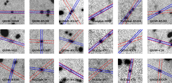
Figure 1.— $\cal R$-band images (rest-frame UV) for our sample of 18 objects. In each image, the NIRSPEC long slit position is overlaid with blue, solid lines. The LRIS slit is overlaid with red, dashed lines. All images are $12^{\prime\prime}$$\times$$12^{\prime\prime}$, with north up and east to the left. Typical seeing during these exposures was $0.^{\prime\prime}8-1.^{\prime\prime}0$.

Our target galaxies were drawn from the UV-selected sample described in Steidel et al. (2003, 2004). These UV-selected surveys have yielded over 3,000 spectroscopically confirmed star-forming galaxies at $z\sim 1.5-3.5$. The majority of the spectra cover the HI Ly$\alpha$ feature at 1216 Å. The observed Ly$\alpha$ profiles for UV-selected star-forming galaxies vary widely in strength, from damped absorption to strong emission. Of the $\sim$1500 objects that show net emission, a fraction exhibit a multiple-peaked profile. While this phenomenon has been previously reported (Tapken et al., 2007; Quider et al., 2009) its frequency of occurrence has never been systematically analyzed. We have used our database of star-forming galaxies to assess the frequency of multiple-peaked Ly$\alpha$ profiles in $z\sim 2-3$ galaxies in order to determine whether such profiles represent rare outliers or are commonplace features of the galaxy population.

To identify the frequency of multiple-peaked profiles, we first separated the full spectroscopic sample into subsets of galaxies with and without detectable Ly$\alpha$ emission. The $\sim$1500 galaxies with Ly$\alpha$ emission were then considered for further study. All of the optical (rest-frame UV) spectra were obtained using the LRIS spectrograph on the Keck I telescope (Oke et al., 1995). These spectra were taken with the 300 line mm^-1 grating blazed at 5000 Å, or, following the LRIS-B upgrade (Steidel et al., 2004), with the 400 line mm^-1 or 600 line mm^-1 grism blazed at 3400 Å, and 4000 Å, respectively. The resolution of the spectra (taken through 1.^′′2 slits) establishes a lower limit in velocity space on the separation of multiple peaks that can be identified. From this sample we were able to identify objects that have a minimum peak separation of 225 [370, 500] km s^-1 for the 600 [400,300]-line grism/grating. We separated the spectra by grism/grating and analyzed each resolution group individually. Approximately 60$\%$ of the spectra were obtained with the 400- and 600-line grisms, while the rest of the spectra were taken using the 300-line grating.

We used a systematic algorithm to search for multiple peaks within the Ly$\alpha$ profile. Several criteria were used to minimize contamination from noisy spectra which can yield a false indication of multiple peaks due to noise spikes. The first criterion was a signal-to-noise (S/N) lower limit of 3 on the strongest flux peak height, which was implemented to establish a consistent threshold for characterizing Ly$\alpha$ profiles. This criterion reduced our sample to $\sim$1000 spectra with 163, 527, and 402 spectra, respectively, from the 600- and 400-line grism, and 300-line grating. The spectra were then separated into resolution groups and the algorithm was implemented independently on each sub-sample. First, we searched between 1210 and 1225 Å in each spectrum for the maximum flux value, given that this wavelength range typically contains the observed Ly$\alpha$ peak in the spectra of star-forming galaxies. This maximum was identified as the primary Ly$\alpha$ emission peak. The continuum level was then estimated for the blue and red side separately from the mean of the flux over a $\sim$100 Å span blueward and redward of 1210 and 1225 Å, respectively. Starting from the primary peak’s maximum flux point, we stepped down towards the blue side until reaching the continuum level. If a local minimum was noted before reaching the continuum we marked the local maximum after that minimum as another possible peak for the Ly$\alpha$ line. Another criterion used to avoid noise spikes was for the secondary maximum to span at least two adjacent steps in wavelength. This procedure was then repeated on the red side of the primary peak. If an additional peak was noted by the algorithm, we required the flux ratio of the additional peak to the primary peak to be greater than $\frac{1}{N}$, with $N$ the S/N of the primary peak. This value was chosen in order to reject any small noise spikes in the identification of the additional peak. Our sample is therefore complete for primary to secondary ratios less than or equal to 3. At higher primary-peak S/N ratio we can also probe larger ratios of primary-to-secondary peak heights. In practice, however, the typical primary-to-secondary peak ratio is $\sim 3$. In addition to analyzing the full sample of spectra with our objective criteria, we examined the spectra by eye for any objects that might have been missed by the algorithm described above. The additional multiple-peaked objects found by eye comprise a small percentage of the total sample, roughly $\sim 15\%$.

For the 300-line grating, the percentage of spectra with multiple-peaked Ly$\alpha$ emission identified is 23$\%$ (92 spectra). For the 600- and 400-line grisms the values are, respectively, 27$\%$ (44 spectra) and 20$\%$ (103 spectra). In addition to the main spectroscopic sample, a set of 121 objects was followed up with 400-line grism spectra using significantly longer exposure times ($7-13$ hours as opposed to 1.5 hours), with correspondingly higher S/N (Bogosavljevic 2010, Ph.D Thesis). In this sample, 97 objects show Ly$\alpha$ emission, and 33$\%$ (32 spectra) of the emitters are identified as containing multiple-peaked Ly$\alpha$ emission using the criteria described above. Higher resolution (i.e., 600-line grism) and S/N (i.e., deeper 400-line grism) spectra are more likely to have identifiable multiple-peaked Ly$\alpha$ emission if it is present. Based on the 600-line and deep 400-line samples we therefore assert that the prevalence of multiple-peaked profiles among objects with Ly$\alpha$ emission is $\sim$30$\%$ in a sample of UV-selected star-forming galaxies at $z\sim 2-3$. This percentage references a S/N lower limit of 3 on the strongest flux peak and a resolution limit of 225 km s^-1.

In order to access the rest-frame optical nebular emission lines (H$\alpha$ at $z\sim 2$ and [OIII]$\lambda$5007 at $z\sim 3$) enabling the determination of systemic velocities for our galaxies, we are restricted to those objects in the full multiple-peaked sample whose redshifts ensure that either H$\alpha$ or [OIII]$\lambda$5007 falls into a window of atmospheric transmission. The sharply increasing thermal background past 2.3 $\mu$m further limits the redshift range over which rest-frame optical emission lines are accessible. In the $\it{K}$-band the available redshift range is $z\sim 2.0-2.6$ for H$\alpha$ and $z\sim 2.9-3.7$ for [OIII]. In the $\it{H}$-band [OIII] can be accessed from $z\sim 1.9-2.6$. After applying the restricted redshift ranges to the multiple-peaked objects determined from the algorithm described above, we identified 193 objects as potential targets for near-infrared spectroscopic follow-up. From this sample we selected the 18 objects described in this paper, which are representative in terms of their Ly$\alpha$ kinematics (see Section 4).

3. Observations and Data Reduction

Both near-IR and optical spectra are required for our analysis of the kinematics of Ly$\alpha$ emission profiles. In this section, we describe both types of spectroscopic data, as well as our basic empirical measurements and uncertainties.

3.1. NIRSPEC Observations and Data Reduction

Near-IR spectra were obtained using the NIRSPEC instrument (McLean et al., 1998) on the Keck II telescope. Our data were collected during three observing runs in 2009 July, August, and October, for a total of 5 nights. On average the total exposure time for each object was 4$\times$900 seconds, though the number of 900 second exposures per target ranged from 3 to 6 for a total integration time of 0.75 to 1.5 hours. All targets were observed with a $0.^{\prime\prime}76$ $\times$ $42^{\prime\prime}$ long slit. For most objects we used the N6 filter, a broad $\it{H+K}$ filter centered at 1.925$\mu$m with a bandwidth of 0.75$\mu$m. For objects at $z\sim 2.5-2.6$, we used the N7 filter, which is centered at 2.23$\mu$m with a bandwidth of 0.80$\mu$m. The spectral resolution as determined from sky lines was $\sim 15$ Å, which corresponds to $\Delta\upsilon\sim$230 km s^-1 (R$\simeq$1300) for the N6 filter and $\Delta\upsilon\sim$200 km s^-1 (R$\simeq$1500) for the N7 filter. Conditions were photometric, with the seeing ranging from $0.^{\prime\prime}33-0.^{\prime\prime}70$.

Due to the faint nature of these objects in the $\it{K}$-band we acquired each target using blind offsets from a bright star in the surrounding field. We returned to the offset star between each integration of the science target to recenter and dither along the slit. In nearly all cases we dithered back and forth between two positions near the center of the slit. The position angle was chosen to match that of the LRIS observation unless the object appeared extended at a different angle in the existing ${\cal R}$-band images (Steidel et al., 2003, 2004). We measured H$\alpha$ or [OIII]$\lambda$5007 for a total of 18 objects during our observing runs, which were drawn from the parent sample discussed in Section 2. All observational information can be found in Table 1. $\cal R$-band images of the objects with the NIRSPEC and LRIS slits overlaid are presented in Figure 1.

Table 1Observation Log with Keck II NIRSPEC

Object	R.A. (J2000)	Dec. (J2000)	$z_{\rm HII}$a,b	$\cal{R}$(mag)	Exposure (s)	Filter	Date (UT)
Q0100-MD40	1 03 18.971	13 17 02.841	2.2506	24.35	4 $\times$ 900	N6	Aug. 09, 2009
Q0100-BX288	1 03 20.931	13 16 23.569	2.1032	23.75	2 $\times$ 900	N6	Aug. 09, 2009
Q0449-BX167	4 52 24.624	-16 39 15.284	2.3557	24.02	4 $\times$ 900	N6	Oct. 10, 2009
Westphal-DD29	14 17 25.936	52 29 32.219	3.2401	24.82	4 $\times$ 900	N6	Aug. 10, 2009
Westphal-BX154	14 17 32.173	52 25 51.044	2.5954	23.96	3 $\times$ 900	N7	July 02, 2009
Q1549-BX102	15 51 55.977	19 12 44.220	2.1932	24.36	3 $\times$ 900	N6	July 01, 2009
Q1549-C20	15 52 00.396	19 08 40.773	3.1174	24.87	3 $\times$ 900	N6	Aug. 10, 2009
Q1549-M22c	15 52 02.703	19 09 40.011	3.1535	24.85	1 $\times$ 900	N6	Jul. 03, 2009
					2 $\times$ 900	N6	Aug. 10, 2009
Q1549-BX202	15 52 05.090	19 12 49.818	2.4831	24.37	4 $\times$ 900	N6	July 01, 2009
Q1623-BX129	16 25 28.732	26 49 19.182	2.3125	24.04	5 $\times$ 900	N6	July 02, 2009
Q2206-BX151	22 08 48.650	-19 42 25.569	2.1974	24.03	4 $\times$ 900	N6	July 01, 2009
SSA22a-D17d	22 17 18.845	0 18 16.667	3.0851	24.27	6 $\times$ 900	N6	July 02, 2009
SSA22a-C49d	22 17 19.810	0 18 18.729	3.1531	23.85	6 $\times$ 900	N6	July 02, 2009
SSA22a-C31	22 17 22.885	0 16 09.492	3.0176	24.61	3 $\times$ 900	N6	July 03, 2009
SSA22a-C32	22 17 25.629	0 16 13.095	3.2926	23.68	4 $\times$ 900	N6	July 03, 2009
Q2343-BX70	23 45 55.934	12 44 50.317	2.4086	24.94	4 $\times$ 900	N6	Aug. 09, 2009
Q2343-BX231	23 46 20.108	12 46 16.812	2.4999	25.15	3 $\times$ 900	N6	Aug. 10, 2009
Q2346-BX181	23 48 31.827	0 21 39.077	2.5429	23.28	3 $\times$ 900	N7	July 01, 2009

Note. — Units of right ascension are hours, minutes, and seconds, and units of declination are degrees, arcminutes and arcseconds.

Data reduction was performed following the method described in Liu et al. (2008), where the sky background was subtracted from the two-dimensional unrectified science images using an optimal method (Kelson, 2003, G. D. Becker 2006, private communication). After background subtraction, cosmic rays and bad pixels were removed from each exposure, which was then rotated, cut out along the slit, and rectified in two dimensions to take out the curvature both in the wavelength and spatial directions. The sky lines were fit with a low-order polynomial and a b-spline fit was used in the dispersion direction. The final rectified two-dimensional exposures for each object were then registered and combined into one spectrum. A one-dimensional spectrum was extracted from the two-dimensional reduced image along with the corresponding 1$\sigma$ error spectrum. The average aperture size along the slit was 2.^′′1, with a range of 1.^′′7 to 2.^′′9. The spectrum was then flux-calibrated using A-type stars observed during our NIRSPEC runs according to the method described in Shapley et al. (2005) and Erb et al. (2003). Finally the flux-calibrated, one-dimensional spectrum was placed in a vacuum, heliocentric frame.

3.1.1 Objects With Spatially-Resolved NIRSPEC Spectra

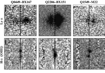
Figure 2.— From left to right, the two-dimensional LRIS and NIRSPEC spectra for Q0449-BX167, Q2206-BX151, and Q1549-M22. These three objects exhibit spatially-extended nebular emission. The horizontal and vertical axes represent, respectively, velocity with respect to the velocity zeropoint and spatial distance along the slit. In each image, the dashed vertical line represents the systemic velocity of the system ($v=0$), and the horizontal axis spans $\pm 1,500$ km s^-1 in velocity. The vertical axes span $\pm 3.5$^′′ in the spatial direction, and a vertical scale bar of $1^{\prime\prime}$ is shown in the upper left-hand panels for Q0449-BX167. (Top) LRIS 2D Ly$\alpha$ spectra. (Bottom) NIRSPEC 2D spectra. The spectra of Q0449-BX167 and Q2206-BX151 show the H$\alpha$ feature, while the spectrum of Q1549-M22 is centered on [OIII]$\lambda$5007. Q0449-BX167 has two components separated by $1.^{\prime\prime}3$ along the slit, Q2206-BX151 is extended spatially by $1.^{\prime\prime}3$, and Q1549-M22 consists of two components separated by $1.^{\prime\prime}1$ in the spatial direction and 130 km s^-1 in the spectral direction.

While the majority of the objects in our sample have spatially unresolved H$\alpha$ (or [OIII]$\lambda$5007) emission-line spectra, three objects exhibit spatially-extended nebular emission: Q0449-BX167, Q2206-BX151, and Q1549-M22. If spatially-extended emission is coupled with rotation or velocity shear, the placement or position angle of the long slit has the potential to yield nebular emission centroid and velocity dispersion values that differ from the true properties of the galaxy. The differences may result if the slit does not evenly sample both the approaching and receding parts of the rotation curve or if systematic shear across the galaxy is interpreted as purely random motions. The three objects listed above were analyzed in more detail to determine whether their complexity might have affected our measurements. In the $\cal R$-band image for Q0449-BX167 there are two distinct components and our slit PA was chosen to have both components included. Q0449-BX167 has two separate components in the two-dimensional NIRSPEC spectrum that are offset in the spatial direction by $1.^{\prime\prime}3$, but not in the spectral direction. In the $\cal R$-band image, Q2206-BX151 is extended and our slit PA was chosen to encompass the extended region. In the two-dimensional NIRSPEC spectrum Q2206-BX151 is extended in the spatial direction for a total of $1.^{\prime\prime}3$. There is a small tail that extends off of the main nebular emission, which is slightly offset in the spectral direction. The flux from the tail is comparable to the noise seen in the image and was not extracted. Since the structure in the two-dimensional spectra for Q0449-BX167 and Q2206-BX151 (excluding the tail) is not shifted in the spectral direction there is no significant evidence for rotation or shear, and the nebular emission centroid and dispersion values for these objects should be robust. In fact, Q0449-BX167 and Q2206-BX151 have among the smallest velocity dispersion values of the sample. The third object, Q1549-M22, is slightly extended in the $\cal R$-band image and again we chose our slit PA to correspond to the extended region. There are two distinct components in the two-dimensional spectrum for Q1549-M22 and they are offset by $1.^{\prime\prime}1$ and 9 Å, respectively, in the spatial and spectral directions. The two-dimensional NIRSPEC spectra for these three objects are presented, along with their corresponding two-dimensional LRIS spectra, in Figure 2.

Object Q0449-BX167 was originally extracted to include only the brighter component on the left hand side of the two-dimensional spectrum. To determine if the spatially-extended nebular emission affects our measurements, we re-extracted Q0449-BX167 to include both components seen in the two-dimensional spectrum. For Q0449-BX167 the centroid did not change and the velocity dispersion changed by $\Delta\sigma_{v}$ = +2.5 km s^-1 when comparing the more extended extraction to our original one. This difference is within our errors. For our analysis we utilize the values obtained from our original extraction of Q0449-BX167. Object Q2206-BX151 was originally extracted to include only the main elongated component. We re-extracted to include the tail for comparison. The centroid of the re-extraction did not change compared to the centroid measured from the original extraction. The velocity dispersion changed from an upper limit of 41 km s^-1 (not including the tail) to a measurement of 63 km s^-1 (including the tail). The re-extractions show that the centroid measurements used in our analysis for Q0449-BX167 and Q2206-BX151 are robust. We include the velocity dispersion values measured from the original extraction for Q2206-BX151 in our analysis with the caveat that the added complexity might affect our modeling comparison (see Section 6).

Our fiducial measurements for Q1549-M22 are based on the extraction of both spectral components. Further analysis was conducted to understand how the spectral offset between the two components might affect our measurements. Each component was extracted and reduced separately for comparison with the integrated extraction of both components. Relative to the velocity zeropoint measured from the summed components, the offsets measured for each component separately are $\Delta v=110$ km s^-1 and $\Delta v=-76$ km s^-1. The measured velocity dispersion of the spectrum integrated over both components (153 km s^-1) is approximately equal to the sum in quadrature of the velocity dispersion of the individual components (125 km s^-1 and 95 km s^-1). The shift from the velocity zeropoint of each component and the large measured velocity dispersion from the summed spectra (the largest in our sample) may be evidence of two separate components giving rise to the two Ly$\alpha$ peaks for this object. We decided to include Q1549-M22 in our sample with the caveat that its complexity in both [OIII]$\lambda$5007 and Ly$\alpha$ may signify a different underlying phenomenon giving rise to the multiple-peaked Ly$\alpha$ emission from the one we will discuss in subsequent sections.

3.2. LRIS Data Reduction

The observations and reduction of the LRIS spectra for our target sample have been described in previous work (Steidel et al., 2003, 2004). These spectra were collected over the course of many years without consistent attention to the accuracy of the zeropoint of the wavelength solution at the 50 to 100 km s^-1 level, given that their primary purpose was for the measurement of redshifts and basic galaxy properties. In contrast, for the work presented here it is crucial to obtain a uniform and highly accurate wavelength zeropoint in order to place our LRIS and NIRSPEC data sets on the same velocity scale. Accordingly, we re-calculated the wavelength solution of each LRIS spectrum. After computing the wavelength solution using the $\tt{IRAF}$ routine $\tt{identify}$ we adjusted the zeropoint of the solution such that bright, unblended sky lines (e.g., $\lambda$5577.339, $\lambda$6300.304) showed up at the correct wavelengths. The spectra were then corrected from an observed, air frame to a heliocentric, vacuum one.

3.3. Line Centroid, Flux, $\&$ FWHM Measurements

Measuring an accurate nebular emission centroid in order to obtain a precise systemic redshift for our objects was the principal objective of the NIRSPEC observations described in Section 3.1. The flux and FWHM were also important measurements for our analysis. The lines that we set out to measure were H$\alpha$ at $z\sim 2$ and [OIII]$\lambda$5007 at $z\sim 3$. The centroid, flux, and FWHM were determined by fitting a Gaussian profile to each emission line using the $\tt{IRAF}$ task, $\tt{splot}$.

A Monte Carlo approach was used to measure the uncertainties in the centroid, flux, and FWHM. For each object 500 fake spectra were created by perturbing the flux at each wavelength of the true spectrum by a Gaussian random number with the standard deviation set by the level of the the 1$\sigma$ error spectrum. Line measurements were obtained from the fake spectra in the same manner as the actual data. The standard deviation of the distribution of measurements from the artificial spectra was adopted as the error on each centroid, flux, and FWHM value. The NIRSPEC measurements and associated uncertainties are given in Table 2. The FWHM values listed are not corrected for instrumental broadening. Based on H$\alpha$ or [OIII]$\lambda$5007 emission line centroid measurements, we obtained the systemic redshifts for our sample. These redshifts were used to shift both the NIRSPEC and LRIS spectra into the systemic rest frame. Based on the Monte Carlo uncertainty of the nebular emission line centroid or the RMS of the wavelength solution (depending on which was greater), we obtain an error of $\Delta\lambda\sim 0.9$ Å, which corresponds to a $\Delta v\sim 10-15$ km s^-1. Repeat observations of two objects from our sample using different slit PAs suggest a larger systematic uncertainty on the order of 50 km s^-1. However, this value should be considered an upper limit on the redshift uncertainty given that we attempted to match the slit positions between NIRSPEC and LRIS observations for a significant fraction of our sample.

Table 2NIRSPEC Measurement Results

Object	$z_{\rm HII}$a	FWHMHIIa,b	$F_{\rm HII}$a,c
Q0100-MD40d	2.2506	14.3 $\pm$ 1.0	3.6 $\pm$ 0.3
Q0100-BX288	2.1032	19.6 $\pm$ 0.4	6.7 $\pm$ 0.1
Q0449-BX167	2.3557	17.3 $\pm$ 1.4	7.8 $\pm$ 0.7
Westphal-DD29	3.2401	22.9 $\pm$ 1.3	22.9 $\pm$ 0.5
Westphal-BX154	2.5954	17.7 $\pm$ 2.0	7.7 $\pm$ 0.8
Q1549-BX102	2.1932	18.2 $\pm$ 1.1	6.1 $\pm$ 0.3
Q1549-C20	3.1174	17.3 $\pm$ 1.0	7.3 $\pm$ 0.4
Q1549-M22	3.1535	29.2 $\pm$ 2.8	8.1 $\pm$ 0.6
Q1549-BX202	2.4831	26.2 $\pm$ 9.9	4.2 $\pm$ 0.9
Q1623-BX129	2.3125	21.1 $\pm$ 2.9	3.5 $\pm$ 0.4
Q2206-BX151e	2.1974	15.7 $\pm$ 0.7	6.3 $\pm$ 0.3
SSA22a-D17	3.0851	25.1 $\pm$ 2.5	2.6 $\pm$ 0.3
SSA22a-C49	3.1531	18.0 $\pm$ 0.6	6.4 $\pm$ 0.2
SSA22a-C31	3.0176	19.7 $\pm$ 1.5	11.5 $\pm$ 0.9
SSA22a-C32d	3.2926	12.8 $\pm$ 35	5.2 $\pm$ 4.7
Q2343-BX70e	2.4086	16.6 $\pm$ 3.5	4.0 $\pm$ 0.6
Q2343-BX231	2.4999	21.5 $\pm$ 1.1	7.2 $\pm$ 0.4
Q2346-BX181	2.5429	28.3 $\pm$ 2.6	13.8 $\pm$ 1.2

4. Ly$\alpha$ Velocity Profiles

Figure 3.— Ly$\alpha$ velocity profiles for the 18 objects in our sample. The zeropoint velocity as measured from the nebular emission (H$\alpha$ at $z\sim 2$ or [OIII]$\lambda$5007 at $z\sim 3$) is indicated on each image with a dashed line. Considerable variety is evident among the line profile peaks and their ratios. From top to bottom and left to right, the panels proceed from Group I to Group V profiles.

Multiple-peaked Ly$\alpha$ emission profiles in $z\sim 2-3$ UV-selected galaxies in principle encode a wealth of information about the velocity and density fields through which they have propagated. It is known that many galaxies at this redshift range are experiencing outflows (Shapley et al., 2003; Veilleux et al., 2005). Simple galactic wind models that incorporate radiative transfer suggest that the specific velocity profile of the resultant Ly$\alpha$ line $\it{relative~{}to~{}systemic}$ can be used to determine parameters of the wind such as the expansion velocity, column density of windswept material, and outflow temperatures (Verhamme et al., 2006, 2008). With our measured systemic redshifts and Ly$\alpha$ morphologies, we are now able to analyze our systems with this comparison in mind. After being shifted to the systemic rest frame based on H$\alpha$ or [OIII] redshifts, the LRIS Ly$\alpha$ spectra were translated from wavelength to velocity space using the rest wavelength of the Ly$\alpha$ feature to create the Ly$\alpha$ velocity profiles. The velocity profiles are shown in Figure 3 and the corresponding velocity measurements for each peak and trough are shown in Table 3.

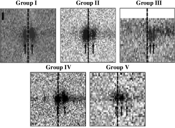
Figure 4.— Two-dimensional Ly$\alpha$ emission spectra representing each of our 5 groups. For each image the horizontal axis represents velocity with respect to the velocity zeropoint, where the dashed vertical line represents the systemic velocity ($v=0$). The horizontal axis in each panel spans $\pm 3,000$ km s^-1. The vertical axis represents spatial distance along the slit, with a span of $\pm 3.5^{\prime\prime}$, and a vertical scale bar of $1^{\prime\prime}$ is shown in the upper left-hand panel (labeled Group I). Group I (two peaks that straddle the velocity-field zeropoint, with the stronger flux peak on the red side) is represented by Westphal-BX154, Group II (two peaks that straddle the velocity-field zeropoint, with the stronger flux peak on the blue side) is represented by Q2346-BX181, Group III (both peaks are shifted completely redward of the zeropoint, with the stronger flux peak on the blue side) by SSA22a-C49, Group IV (two peaks that straddle the velocity-field zeropoint with both peaks having approximately the same flux with the red peak marginally stronger) by SSA22a-D17, and Group V (three peaks) by Q1623-BX129. In each panel, the locations of the Ly$\alpha$ peaks are indicated by arrows.

Table 3Velocity Measurements from Ly$\alpha$ Emission and Interstellar Absorption

Object	$z_{\rm HII}$a	First Peakb	Second Peakb	Troughb	Absorptionb	Grism/Gratingc
Q0100-MD40d	2.2506	$-461$	$+550$	$+288$	$-19$	600, 400
Q0100-BX288	2.1032	$-579$	$+377$	$-104$	$-317$	400
Q0449-BX167	2.3557	$-348$	$+586$	$-60$	$-47$	400
Westphal-DD29	3.2401	$-259$	$+471$	$+202$	$\cdot\cdot\cdot$	300
Westphal-BX154	2.5954	$-353$	$+404$	$-27$	$-204$	600
Q1549-BX102	2.1932	$-478$	$+264$	$-155$	$\cdot\cdot\cdot$	600
Q1549-C20	3.1174	$-237$	$+533$	$+210$	$+14$	400
Q1549-M22	3.1535	$-153$	$+414$	$+111$	$\cdot\cdot\cdot$	600
Q1549-BX202	2.4831	$-542$	$+301$	$-141$	$-143$	600
Q1623-BX129e	2.3125	$-42$	$+542$	$+229$	$-468$	400
Q2206-BX151	2.1974	$-417$	$+328$	$-148$	$\cdot\cdot\cdot$	600
SSA22a-D17	3.0851	$-25$	$+732$	$+385$	$-1174$	400
SSA22a-C49	3.1531	$+518$	$+903$	$+735$	$-232$	400
SSA22a-C31	3.0176	$-15$	$+695$	$+424$	$\cdot\cdot\cdot$	300
SSA22a-C32	3.2926	$-155$	$+493$	$+99$	$-24$	400
Q2343-BX70	2.4086	$-476$	$+399$	$-214$	$-33$	400
Q2343-BX231	2.4999	$+84$	$+567$	$+399$	$\cdot\cdot\cdot$	400
Q2346-BX181	2.5429	$-214$	$+626$	$+338$	$-49$	400

The Ly$\alpha$ velocity profiles can be separated into groups characterized by the strengths and locations of the emission peaks with respect to the velocity-field zeropoint. The majority of objects in our sample (11/18), which we refer to as Group I, have two peaks that straddle the velocity-field zeropoint, with the stronger flux peak on the red side. This group includes objects Q0100-MD40, Q0100-BX288, Q0449-BX167, Westphal-DD29, Westphal-BX154, Q1549-BX102, Q1549-M22, Q1549-BX202, Q2206-BX151, SSA22a-C32, and Q2343-BX70. In the case of Q1549-M22, the object with two apparently distinct spectral and spatial [OIII] emission components, regardless of whether we shift the velocity-field zeropoint to $\Delta v=110$ km s^-1 or $\Delta v=-76$ km s^-1, as measured from the re-extraction of each component individually, both Ly$\alpha$ peaks still straddle the zeropoint. Therefore Q1549-M22 is classified as a Group I object independent of the adopted velocity zeropoint. Group II spectra, including objects Q1549-C20 and Q2346-BX181, are described by two peaks that straddle the velocity-field zeropoint, and have the stronger flux peak on the blue side. Objects Q2343-BX231 and SSA22a-C49 comprise Group III, where the bluer Ly$\alpha$ peak is stronger, but unlike the profiles previously described, both peaks are shifted completely redward of the zeropoint. Group IV, SSA22a-D17 and SSA22a-C31, have two peaks that straddle the velocity-field zeropoint with both peaks having approximately the same flux with the red peak marginally stronger. Object Q1623-BX129 accounts for the last group, Group V. This object has three peaks. Two of the peaks are similar to those of SSA22a-D17 and SSA22a-C31, with nearly the same flux and one on either side of the zeropoint. The third peak, which is furthest redward from the zeropoint, has the smallest flux. Examples of two-dimensional Ly$\alpha$ spectra from each group are displayed in Figure 4.

A precise velocity-field zeropoint in addition to the velocity dispersion (see Section 5.1) provides constraints on radiative transfer models of the Ly$\alpha$ emission from our sample of galaxies (see Section 6). Figure 5 shows a graphical summary of peak velocities along with the relative fluxes of each peak for every galaxy in our sample. Additionally, some objects have detectable interstellar absorption lines, which are also labeled on Figure 5. The analysis of the absorption lines is described in Section 5.4. The velocity separation of the peaks in the Ly$\alpha$ profiles is also an important constraint on possible models. The mean velocity peak separation is $\langle\Delta v_{peak}\rangle=741\pm 39$ km s^-1 (where the error represents the standard deviation of the mean), and the median is $\Delta v_{peak,med}$ = 757 km s^-1.

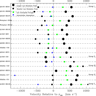
Figure 5.— The location of the velocity for every peak, trough, and absorption line with respect to the velocity-field zeropoint. From top to bottom, the properties are displayed for Group I, II, III, IV, and V objects. Objects are offset vertically for clarity. In each line the larger [smaller] black dot represents the velocity peak with the larger [smaller] flux. The green square represents the velocity of the trough between the peaks. The blue triangle represents the absorption line velocity if it was measured for the object. For Q1623-BX129, which has three measured peaks, an even smaller black dot is used to indicate the third peak with the weakest flux.

An examination of the parent LRIS multiple-peaked sample indicates the same trends as described above. Analyzing the objects in the parent sample with a S/N lower limit of 3 on the strongest flux peak reveals that $\sim$65$\%$ have their strongest flux peak located on the red side of the interpeak trough (compared to 72$\%$ from the NIRSPEC sample). Despite a wide range from minimum to maximum for the peak-to-peak velocity separation, the statistics for the parent LRIS sample are comparable to those for our NIRSPEC sample, with a mean value of $\langle\Delta v_{peak}\rangle=$ 723 $\pm$ 18 km s^-1 (where the error represents the standard deviation of the mean), and a median of $\Delta v_{peak,med}=$ 721 km s^-1. Figure 6 shows the distributions of peak-to-peak velocity separation for our NIRSPEC sample and the parent LRIS sample. These distributions demonstrate that our sample of 18 objects with NIRPSEC observations is representative of the parent LRIS sample as a whole.

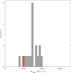
Figure 6.— Histogram of the distribution of peak-to-peak velocity separation. (Left) The histogram for the 18 objects with NIRSPEC measurements. The red shaded bar represents the separation of the 2nd peak (the center peak) from the 3rd peak (the reddest peak) for object Q1623-BX129. The mean value for the sample is $\langle\Delta v_{peak}\rangle=741\pm 39$ km s^-1, with a median of $\Delta v_{peak,med}=757$ km s^-1. (Right) Histogram of the peak-to-peak separation for our parent LRIS sample with a S/N lower limit of 3. The mean value is $\langle\Delta v_{peak}\rangle=723\pm 18$ km s^-1, with a median of $\Delta v_{peak,med}=721$ km s^-1.

5. Physical Quantities

In this section, we discuss several relevant physical properties for the NIRSPEC multiple-peaked sample objects that can be estimated from our combined dataset.

5.1. Velocity Dispersion

As traced by H$\alpha$ (or [OIII]$\lambda$5007) emission, the nebular velocity dispersion, $\sigma_{v}$, reflects the integrated emission from star forming regions, which should reveal the potential well within the central few kiloparsecs of a high-redshift star-forming galaxy. Since the H$\alpha$ (or [OIII]$\lambda$5007) velocity dispersion also traces the initial velocity dispersion of the Ly$\alpha$ photons, it is an important input parameter for models of Ly$\alpha$ radiative transfer and will enable a better understanding of the multiple-peaked Ly$\alpha$ emission systems in our sample. In this paper, aside from a brief comparison with previous work (Section 6.2), we do not include a detailed analysis of the relationship between intrinsic velocity dispersion and the emergent Ly$\alpha$ profile. Such analysis is deferred to future work, as discussed in Section 7.

The velocity dispersion was calculated as $\sigma_{v}$ $=$ (FWHM/2.355) $\times(c/\lambda_{obs})$, where $\lambda_{obs}$ is the observed wavelength of H$\alpha$ or [OIII]$\lambda$5007. The FWHM is determined from the subtraction of the instrumental FWHM (estimated from the widths of night sky lines) from the observed FWHM in quadrature. Uncertainties in the velocity dispersion were determined using the same method described in Erb et al. (2006b). Of our 18 objects, 14 have measurable velocity dispersion. For 2 additional objects we obtained an upper limit in the velocity dispersion because the measured line width was not appreciably higher than the instrumental resolution. Finally, 2 objects have measured line widths that are smaller than the instrumental resolution and are therefore considered unresolved. Figure 7 shows the distribution of the velocity dispersion for the sample. The mean value for the sample of 14 objects with measurable velocity dispersion is $\langle\sigma_{v}\rangle$ = 90$\pm$ 9 km s^-1 (where the error represents the standard deviation of the mean), while the median for the full sample of 18 objects is $\sigma_{v,med}$= 82 km s^-1. These are similar to the typical values reported by Erb et al. (2006b) and Pettini et al. (2001) for $z\sim 2-3$ UV-selected galaxies ($\sigma_{v}=108\pm 5$ km s^-1 for $z\sim 2$ and $\sigma_{v}=84\pm 5$ km s^-1 for $z\sim 3$).

5.2. Dust Extinction

Ly$\alpha$ emission can be significantly suppressed due to attenuation by dust. Commonly, dust extinction in $z\sim 2$ star-forming galaxies is estimated from rest-frame UV colors and an assumption of the Calzetti et al. (2000) starburst attenuation law. Alternatively, the amount of dust extinction can be estimated from the observed ratio of hydrogen Lyman to Balmer lines, since their intrinsic ratios are well described by atomic theory. An assumption of Case B recombination and $T=10,000K$ determines the intrinsic Ly$\alpha$ to H$\alpha$ ratio (Osterbrock, 1989). Any deviation from this value is then attributed to dust extinction. In our sample, only 11 of 18 galaxies have measured H$\alpha$ (the remainder have [OIII]$\lambda$5007), making the first method more generally applicable for our analysis. Both methods were used to calculate $E(B-V)$ for objects with measured H$\alpha$.

For the first method, we used the $G-\cal R$ colors of our sample as determined from Steidel et al. (2003, 2004). If the Ly$\alpha$ line fell in the $G$-band (at $z\sim 2.48-3.28$) the color was corrected for emission-line contamination using $\Delta m=2.5\times\log(1+\frac{EW}{\Delta G})$, where $\frac{EW}{\Delta G}$ is the ratio of the observed equivalent width of the Ly$\alpha$ emission feature to the bandwidth of the $G$ filter (1100 Å). The correction, $\Delta m$, was then added to the $G-\cal R$ color. The $G-\cal R$ color for objects at $z>2.45$ was also corrected for IGM absorption in the $G$-band (Madau, 1995). An intrinsic SED model was assumed as well to estimate the dust extinction. We used a Bruzual & Charlot (2003) model assuming solar metallicity and constant star formation rate with a stellar age of 570 Myr for $z\sim 2$ and 202 Myr for $z\sim 3$ objects. Our choice of stellar age for objects at $z\sim 2$ was based on results from Erb et al. (2006b), who found a median age of 570 Myr for star-forming galaxies in this redshift range. The stellar age of 202 Myr adopted for the $z\sim$3 galaxies was based on results from Shapley et al. (2005). The calculated values of $E(B-V)$ are listed in Table 4.

For the second method, based on the ratio of Ly$\alpha$ and H$\alpha$ emission lines, we adopt the flux ratio $\frac{Ly\alpha_{(int)}}{H\alpha_{(int)}}=8.7$ (Osterbrock, 1989). We used the following equation:

$$\frac{Ly\alpha_{(obs)}}{H\alpha_{(obs)}}=8.7\times 10^{-0.4E(B-V)(\kappa_{Ly\alpha}-\kappa_{H\alpha})}$$ (1)

In this equation $\kappa_{Ly\alpha}$ and $\kappa_{H\alpha}$ refers to the selective extinction at the wavelengths of Ly$\alpha$ and H$\alpha$, respectively, as defined in Equation 4 of Calzetti et al. (2000). $E(B-V)$ can then be calculated based on the observed ratio of Ly$\alpha$ to H$\alpha$ flux. All of our calculated $E(B-V)$ values from this method exceed those measured from the rest-frame UV colors, and the median excess is a factor of 1.5. This difference may be explained with reference to Calzetti et al. (2000), which states that the stellar continuum in local star-forming galaxies should suffer less reddening than the ionized gas. Furthermore, Ly$\alpha$ may suffer additional extinction due to resonant scattering and an effectively longer path length though the interstellar medium. In practice, it is difficult to obtain a robust estimate of the Ly$\alpha$ to H$\alpha$ ratio due to the effects of differential slit loss. Erb et al. (2006a) find that NIRSPEC H$\alpha$ spectra using the 0.76^′′ slit may result in a typical factor of $\sim$2 loss, while Steidel et al. (2011) find that LRIS 1.2^′′ slit spectra of Ly$\alpha$ may result in typical losses of a factor of $\sim$5. In detail, the relative loss of Ly$\alpha$ to H$\alpha$ depends on the spatial distribution of the emission in each of these lines. Overall, the Ly$\alpha$ losses appear to outweigh those of the H$\alpha$ losses, which will tend to cause an underestimate in the Ly$\alpha$ to H$\alpha$ ratio. Because of the systemic uncertainty of the Ly$\alpha$ to H$\alpha$ ratio and due to the fact that we can only estimate $E(B-V)$ for half of the sample using the (uncertain) intrinsic ratio method, we adopt the values calculated from the rest-frame UV colors. The average value for our sample when employing the first method is $\langle E(B-V)\rangle$ = 0.09, which is bluer than the typical value seen at these redshifts, $\langle E(B-V)\rangle$ = 0.15 (Reddy et al., 2008). This difference is not surprising given that our sample is entirely composed of objects with Ly$\alpha$ emission and given the apparent anti-correlation between Ly$\alpha$ emission EW and dust extinction (Shapley et al., 2003; Kornei et al., 2010).

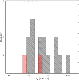
Figure 7.— Histogram of the nebular velocity dispersion, $\sigma_{v}$, as traced by H$\alpha$ or [OIII]$\lambda$5007 measurements. The measurements for two objects with FWHM not appreciably larger than the instrumental resolution, Q2206-BX151 and Q2343-BX70, are shaded red. The two objects that are considered unresolved, Q0100-MD40 and SSA22a-C32, are not included in this figure. The mean value for the sample of 14 objects with measured velocity dispersions is $\langle\sigma_{v}\rangle=$ 90$\pm$ 9 km s^-1. The median value for the full sample of 18 objects is $\sigma_{v,med}=$ 82 km s^-1.

5.3. Star-Formation Rates and Intrinsic Luminosity

Star-formation rates were calculated from the rest-frame UV luminosity. For sources at $z\sim 2$ we used the $G$-band as a proxy for rest-frame UV luminosity. At $z\sim 3$, $\cal R$-band is used as an equivalent probe. The observed magnitudes were first corrected for dust extinction using $m_{corr}=m_{app}-(\kappa\times E(B-V))$, where $\kappa$ is defined in Section 5.2. Given the range of redshifts in our $z\sim 2$ sample the $G$-band effective wavelength of 4780 Å corresponds to a rest-frame wavelength range of $1330-154$0 Å. For the $z\sim 3$ sample the $\cal R$-band effective wavelength translates to a rest-frame effective wavelength of $1590-1700$ Å. These rest-frame wavelengths were used to determine $\kappa$ values. The corrected magnitude was then used to determine the flux, $F_{\nu}$. Using the luminosity distance, we calculated the rest-frame UV luminosity density according to $L_{\nu}=(4\pi{D_{L}}^{2}F_{\nu})/(1+z)$. From Kennicutt (1998a), the relation of $\mbox{SFR}(M_{\odot}$ yr${}^{-1})=7.8\times 10^{-29}$ $L_{\nu}$(ergs s^-1 Hz^-1) was used to determine the SFRs assuming a Chabrier (2003) IMF. The SFRs for the sample range from 6$-$110 $M_{\odot}$ yr^-1. The average value is 32 $M_{\odot}$ yr^-1, which is fairly typical of UV-selected star-forming galaxies at $z\sim 2-3$ (Erb et al., 2006a). The intrinsic Ly$\alpha$ luminosity, $L_{Ly\alpha}$, can be derived from the SFR using the conversion described in Kennicutt (1998b) and again assuming a Chabrier (2003) IMF:

$$L_{Ly\alpha}(\mbox{ergs}~{}\mbox{s}^{-1})=\frac{\mbox{SFR}~{}(M_{\odot}~{}\mbox{yr}^{-1})}{5.1\times 10^{-43}}$$ (2)

Based on the average SFR of 32 $M_{\odot}$ yr^-1, the intrinsic Ly$\alpha$ luminosity is $\langle L_{Ly\alpha}\rangle=6.3\times 10^{43}$ ergs s^-1. The intrinsic Ly$\alpha$ luminosity is an important quantity for our models because it allows us to input an accurate description of the photon source from our galaxies. SFRs and $L_{Ly\alpha}$ values are listed in Table 4.

Table 4Physical Quantities

Object	$\sigma_{v}~{}^{a}$	$E(B-V)$   b	SFRc	$L_{{\rm Ly}\alpha}$d
Q0100-MD40	$\cdot\cdot\cdot$	0.00	6	1.25
Q0100-BX288	84.8${}^{+3}_{-3}$	0.02	11	2.16
Q0449-BX167	50.3${}^{+14}_{-19}$	0.20	51	10.10
Westphal-DD29	102.5${}^{+10}_{-11}$	0.00	73	14.90
Westphal-BX154	52.4${}^{+18}_{-24}$	0.26	110	21.70
Q1549-BX102	64.6${}^{+10}_{-13}$	0.10	13	2.51
Q1549-C20	55.2${}^{+11}_{-13}$	0.04	9	1.83
Q1549-M22	153.1${}^{+19}_{-20}$	0.15	27	5.23
Q1549-BX202	119.7${}^{+63}_{-84}$	0.07	14	2.78
Q1623-BX129	89.5${}^{+22}_{-25}$	0.00	9	1.74
Q2206-BX151	$<$ 40.5	0.01	8	1.66
SSA22a-D17	124.9${}^{+19}_{-20}$	0.08	24	4.84
SSA22a-C49	60.5${}^{+6}_{-7}$	0.07	33	6.61
SSA22a-C31	82.0${}^{+14}_{-15}$	0.00	8	1.59
SSA22a-C32	$\cdot\cdot\cdot$	0.04	31	6.19
Q2343-BX70	$<$ 78.5	0.13	12	2.35
Q2343-BX231	86.3${}^{+8}_{-9}$	0.29	47	9.20
Q2346-BX181	131.8${}^{+17}_{-17}$	0.18	97	19.20

5.4. Interstellar Absorption

The evidence for feedback in high-redshift galaxies comes in several forms, one of which is the nature of rest-frame UV interstellar absorption lines. Interstellar material is swept up in a galaxy-wide outflow, causing a blueshift in the associated absorption lines. In our sample over half of the objects have detected interstellar absorption lines. These include both low-ionization (Si II$\lambda$1260, Si II$\lambda$1526, and C II$\lambda$1334) and high-ionization (Si IV$\lambda\lambda$1393,1402 and C IV$\lambda\lambda$1548,1549) lines.

For all but two objects the absorption lines identified in the spectra are low-ionization species. The S/N of these lines is not exceptionally strong on an individual basis. In principle, all of the low-ionization lines arise in the same gas and should share the same $z_{abs}$ and velocity profiles. Based on this idea we continuum-normalized and averaged the Si II$\lambda$1260, Si II$\lambda$1526, and C II$\lambda$1334 velocity profiles to obtain better S/N. Figure 8 shows an example of one of our objects, Westphal-BX154, with averaged low-ionization lines, as well as object SSA22a-C49, which has measurements of both low- and high-ionization lines. The velocity offsets in our sample measured from the absorption line centroids range from $\Delta v_{abs}=+14$ to $-1,174$ km s^-1, relative to the systemic velocity. The average value of the interstellar absorption velocity offset for the sample is $\langle\Delta v_{abs}\rangle=-227$ km s^-1, which is indicative of large scale outflows (Pettini et al., 2001; Shapley et al., 2003; Steidel et al., 2010).

Figure 8.— Interstellar absorption velocity profiles for two objects in our sample. Interstellar absorption lines were measured for 12 out of the 18 objects in our sample, and the majority have centroids that are blueshifted relative to the velocity zeropoint. (Left) Comparison of the Ly$\alpha$ and low- and high-ionization interstellar absorption velocity profiles for SSA22a-C49. All of the absorption-line velocity centroids appear blueward of the velocity-field zeropoint, whereas the Ly$\alpha$ velocity profile is shifted completely redward of the velocity-field zeropoint. (Right) Comparison of the Ly$\alpha$ and averaged low-ionization interstellar absorption velocity profiles of Westphal-BX154. The low-ionization lines, Si II$\lambda$1260, Si II$\lambda$1526, and C II$\lambda$1334, were averaged to obtain better S/N. The absorption line velocity centroid is blueshifted relative to the velocity-field zeropoint. The two peaks of the Ly$\alpha$ velocity profile straddle the velocity-field zeropoint.

Figure 9.— Histogram of interstellar absorption line widths, $\sigma_{abs}$. All $\sigma_{abs}$ values were measured from the combined low-ionization lines for each object, except for SSA22a-C32, SSA22a-C49 and SSA22a-D17, where individual low-ionization lines were measured and then averaged. The mean value of the sample is $\langle\sigma_{abs}\rangle=$ 190 $\pm$ 63 km s^-1. The line width is an important parameter for modeling Ly$\alpha$ radiative transfer because it reveals the dynamics of the absorbing interstellar gas.

The line width of the interstellar absorption features was measured as $\sigma_{abs}=$ (FWHM/2.355) $\times(c/\lambda_{obs})$, where $\lambda_{obs}$ is the observed wavelength of the interstellar absorption line. The FWHM was corrected for instrumental resolution ($\sigma_{inst}=$ (FWHM_inst/2.355) = 95, 155, 190 km s^-1 for the 600, 400, 300-line grism, respectively). The line width, $\sigma_{abs}$, is a probe of the range of velocities present in the interstellar gas, which is an important observational constraint for Ly$\alpha$ radiative transfer models (see Section 6). The average $\sigma_{abs}$ for the 12 objects in our sample with absorption line measurements is 190 $\pm$ 63 km s^-1 (where the error represents the standard deviation of the distribution of measurements). This line width is consistent with measurements made by Shapley et al. (2003) of $\langle\sigma_{abs}\rangle$ = 238 $\pm$ 64 km s^-1 in a composite spectrum of 811 $z\sim 3$ Lyman Break Galaxies (LBGs) and Quider et al. (2009) of $\sigma_{abs}\sim$ 170$-$255 km s^-1 in the strong gravitationally lensed galaxy, “the Cosmic Horseshoe”, at $z=2.38$. Our $\sigma_{abs}$ values were measured from the combined low-ionization lines for each object except for SSA22a-C32, SSA22a-C49 and SSA22a-D17, where individual low-ionization lines were measured and then averaged. Figure 9 shows the distribution of the interstellar absorption line widths for our sample.

We also investigated if there was an inherent difference in the interstellar absorption line profiles for multiple-peaked compared to single-peaked Ly$\alpha$ emission spectra. For this comparison we constructed composite LRIS rest-frame UV spectra for our sample of 18 multiple-peaked objects and for a sample of 29 galaxies from Steidel et al. (2010) with single-peaked Ly$\alpha$ emission profiles and precisely measured systemic redshifts based on NIRSPEC observations of H$\alpha$. To create the composite spectrum we utilized the $\tt{IRAF}$ routine, $\tt{scombine}$, computing the average of the rest-frame spectra at each wavelength with a minimum/maximum pixel rejection. The composite spectrum was then continuum normalized using a cubic spline fitting function. The Ly$\alpha$ profile in the composite spectrum of our sample is characterized by two clear peaks, with a stronger peak on the red side. This profile is expected since the majority of our profiles resemble such a configuration (i.e. Group I). For the single-peaked composite spectrum, the measured line widths of the interstellar absorption lines are systematically larger than those in the multiple-peaked composite spectrum, with $\langle\sigma_{abs}\rangle=140\pm 26$ km s^-1 for the multiple-peaked composite and $\langle\sigma_{abs}\rangle=220\pm 19$ km s^-1 for the single-peaked composite. The line widths, $\langle\sigma_{abs}\rangle$, were calculated from the averaged Si II$\lambda$1260 and C II$\lambda$1334 lines, which were chosen because of their higher S/N. A Monte Carlo approach, similar to the one described in Section 3.3, was used to estimate the error. This difference in interstellar absorption linewidths may indicate that the range of velocities found within the interstellar gas must be narrower in order to create a multiple-peaked profile instead of a single-peaked profile. A comparison of Ly$\alpha$ emission profiles indicates that the centroid of the Ly$\alpha$ emission peak in the single-peaked composite is the same as the centroid of the redder peak in the multiple-peaked composite spectrum. Figure 10 illustrates the differences between the total and Group I composite spectra from our sample and the stack of the 29 single-peaked Ly$\alpha$ emission objects from Steidel et al. (2010). We note here that only two out of the 29 single-peaked spectra included in the single-peaked composite were taken with the 600-line grism, while 600-line spectra comprise 5 out of 18 in the multiple-peaked composite. To determine if a possible second peak was missed in the single-peaked composite due to decreased resolution, we smoothed the multiple-peaked composite to the resolution to the single-peaked composite. The second peak in the multiple-peaked composite is still distinctly evident after smoothing, demonstrating that the observed multiple-peaked phenomenon is not simply a result of better resolution. Also of note is the fact that the redshift distribution for our multiple-peaked spectra is bimodal (with objects at $z\sim 2.1-2.6$ and $z\sim 3.0-3.3$) and characterized by a mean value of $\langle z\rangle=2.67\pm 0.42$, with a median of $z=2.54$. The redshift distribution for the single-peaked spectra has $\langle z\rangle=2.31\pm 0.13$, with a median of $z=2.31$. To control for any possible effects of redshift evolution, we also compare the subset of $z\sim 2$ objects with the single-peaked spectra, and find the same spectral trends.

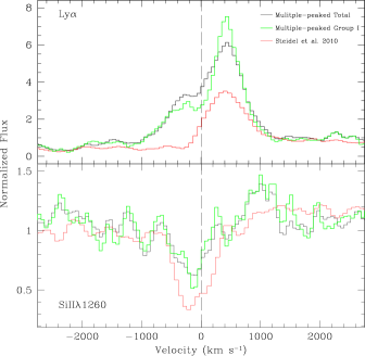
Figure 10.— Comparison of velocity profiles for the composite of the 18 multiple-peaked objects with NIRSPEC measurements, the subset of 11 objects that comprise Group I, and 29 single-peaked spectra from Steidel et al. (2010). (Top) The Ly$\alpha$ velocity profile for each composite spectrum. The emission centroid from the single-peaked composite spectrum matches the centroid of the red peak from both of the double-peaked composite spectra. (Bottom) The interstellar absorption velocity profile of Si II$\lambda$1260 for each composite spectrum. The line widths for the single-peaked profile ($\langle\sigma_{abs}\rangle=220\pm 19$ km s^-1) are systematically larger than for the multiple-peaked profile ($\langle\sigma_{abs}\rangle=140\pm 26$ km s^-1). The line width for the Group I composite is $\langle\sigma_{abs}\rangle=100\pm 31$ km s^-1. The interstellar absorption lines are also inherently deeper for the single-peaked compared to the multiple-peaked composite.

Finally, the interstellar absorption line kinematics allow us to consider the possibility of an alternate scenario for a multiple-peaked Ly$\alpha$ emission profile. The multiple-peaked nature of Ly$\alpha$ emission can also be explained in terms of the interpeak trough tracing absorption from neutral HI with the same kinematics as the material giving rise to the interstellar metal absorption lines. According to this scenario, the trough and the interstellar absorption centroids would be aligned in velocity space. Figure 5 shows that, with the possible exception of Q1549-BX202 and Q0449-BX167, the Ly$\alpha$ trough velocity centroid does not line up with the interstellar absorption centroid for any of the objects in our sample with interstellar absorption measurements – ruling out this possible hypothesis.

6. Ly$\alpha$ Radiative Transfer Modeling

6.1. Models

Explaining the emergent profile of Ly$\alpha$ emission in star-forming galaxies has been the subject of many theoretical and observational studies because of the easy observability of the Ly$\alpha$ line and the complex processes that govern how it emerges from galaxies. Models for the propagation and escape of Ly$\alpha$ photons have been based on both Monte Carlo radiative transfer and simple analytic calculations for a variety of idealized gas density and velocity distributions (Hansen & Oh, 2006; Steidel et al., 2010; Verhamme et al., 2006, 2008) as well as post-processing of 3D cosmological hydrodynamical simulations (Laursen et al., 2009a; Barnes et al., 2011). For analytic models, the gas density and velocity distributions assumed include static, expanding, and infalling shells with both unity and non-unity covering fraction, expanding and infalling uniform-density haloes in which the gas velocity depends monotonically on galactocentric distance, open-ended tubes, and spherical distributions of discrete clouds with a range of velocity profiles. In some of these models, the effect of dust extinction has been treated explicitly (Verhamme et al., 2006, 2008; Hansen & Oh, 2006; Laursen et al., 2009b).

One of the simple models that has been most closely compared with individual LBG spectra is that of an expanding shell of gaseous material (Verhamme et al., 2006, 2008; Schaerer & Verhamme, 2008). In this picture, energy from supernova explosions sweeps up the ISM of star-forming galaxies into a geometrically thin but optically thick spherical shell. With the advent of efficient algorithms to perform resonant-line radiative transfer, it has been shown that such a system can be made to reproduce the observed Ly$\alpha$ profiles of high-redshift galaxies (Verhamme et al., 2006, 2008). Verhamme et al. (2006) deconstruct the Ly$\alpha$ line morphology in order to determine how specific features in the Ly$\alpha$ profile can be related to physical parameters of model systems as well as specific photon trajectories. For example, a shell expanding with uniform velocity $V_{\rm exp}$ will produce a primary redshifted peak at approximately $v=2V_{\rm exp}$ corresponding to photons that have undergone a single backscattering event en route to the observer. Photons that undergo zero backscatterings emerge in an asymmetric double-peaked structure centered about a velocity $v=-V_{\rm exp}$. Finally, photons that experience multiple backscattering events emerge redward of the primary peak. At fixed expansion velocity, the red-side peaks become indistinguishable from one another and the blue-side peak becomes more blueshifted as the Doppler parameter, $b$, increases. Increasing the column density but keeping the expansion velocity and thermal velocity fixed results in an enhanced inter-peak separation and broader peaks. Verhamme et al. (2006) also consider the effect of dust attenuation on the emergent Ly$\alpha$ profile, showing how it can reduce the overall Ly$\alpha$ escape fraction, as well as modulate the shape of the profile in velocity space.

6.2. Comparison Between Models and Observations

In order to investigate whether such a system can reproduce the data presented here, we use the radiative transfer code developed in Zheng & Miralda-Escudé (2002) and Kollmeier et al. (2010) to generate the observed Ly$\alpha$ spectra emerging from expanding/infalling shell models similar to those presented in Verhamme et al. (2006), with a range of shell column densities, expansion velocities and Doppler parameters. Figure 11 shows a subset of such models, for a central monochromatic source of Ly$\alpha$ photons propagating outward through an expanding shell with a column density of $N_{HI}=2\times 10^{20}\mbox{ cm}^{-2}$, expansion velocities of $V_{\rm exp}=$ 100, 300, and 400 km s^-1, and Doppler $b$-parameters of 40, 80, 120, and 250 km s^-1. It should be noted that the Ly$\alpha$ radiative transfer calculation does not depend on the exact physical dimensions of the system for a given column density, expansion velocity, and Doppler parameter as long as the shell is kept geometrically thin. The models have been smoothed to the typical resolution of our LRIS data, for a fair comparison with the observations. Future modeling (Kollmeier et al., in prep.) will include a distribution of injection frequencies for Ly$\alpha$ photons that matches the nebular velocity dispersions measured from H$\alpha$ and [OIII], as well as a more extensive set of gas density and velocity distributions for radiative transfer calculations.

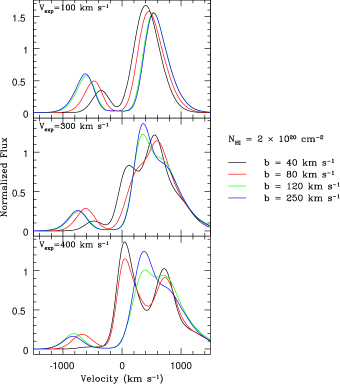
Figure 11.— Emergent Ly$\alpha$ profiles from an expanding shell with a central monochromatic source. In all panels, the hydrogen column density of the expanding shell is $N_{HI}=2\times 10^{20}\mbox{ cm}^{-2}$. The top, middle, and bottom panels show the emergent profiles for shells with expansion velocities of, respectively, $V_{\rm exp}=$100, 300, and 400 km s^-1. In each panel, black, red, green, and blue curves respectively indicate profiles for Doppler parameters of $b=$40, 80, 120, and 250 km s^-1. Each predicted model curve has been smoothed to the typical resolution of our LRIS spectra.

By far the most common Ly$\alpha$ profile observed within the NIRSPEC multiple-peaked sample is the “Group I” type, with two peaks straddling the velocity-field zeropoint, and a stronger red-side peak. Given the frequency of this profile type, it is of particular interest to compare it with Ly$\alpha$ radiative transfer models. In addition to the Ly$\alpha$ emission properties, we mention here that the typical low-ionization interstellar absorption blueshift for Group I objects is slightly smaller than the sample average, with $\langle\Delta v_{abs}\rangle_{\mbox{Group I}}=-90$ km s^-1 (based on the 7 out of 11 Group I objects with interstellar absorption line measurements). The average low-ionization interstellar absorption line width for Group I objects is $\langle\sigma_{abs}\rangle\sim 160$ km s^-1, corresponding to $b=226$ km s^-1, if the line width is interpreted as the thermal velocity of a single expanding component of gas (which may indeed not be the correct interpretation of the interstellar absorption profiles, see, e.g., Steidel et al., 2010, and Section 6.3). As seen in Figure 11, the best match with the typical Group I profile is obtained using the $N_{HI}=2\times 10^{20}\mbox{ cm}^{-2}$, $V_{\rm exp}=100$ km s^-1, $b=40$ km s^-1 model. In this model, which also features two peaks straddling the velocity-field zeropoint and a stronger red peak, the blue peak appears at $\Delta v=-370$ km s^-1, while the red peak appears at $\Delta v=+430$ km s^-1. The model matches the average Group I properties both in terms of the locations of the Ly$\alpha$ peaks relative to zero, as well as the interpeak separation, although the predicted contrast between the red and blue peak heights is too large. At the same time, the predicted absorption profile for such an expanding shell (which should be traced well by the low-ionization features arising in neutral hydrogen gas) would have $\langle\sigma_{abs}\rangle\sim b/\sqrt{2}\sim 30$ km s^-1, i.e., significantly lower than what is observed for Group I objects. This difference represents a fundamental discrepancy between the shell model and the full complement of Group I data – even if the average Ly$\alpha$ emission profile can be roughly reproduced. Figure 12 shows the $N_{HI}=2\times 10^{20}\mbox{ cm}^{-2}$, $V_{\rm exp}=100$ km s^-1, $b=40$ km s^-1 model, along with other $V_{\rm exp}=100$ km s^-1 expanding shell models with smaller column density (i.e., $N_{HI}=1\times 10^{17}\mbox{ cm}^{-2}$ or $N_{HI}=1\times 10^{19}\mbox{ cm}^{-2}$) and larger Doppler parameters ($b\geq 120$ km s^-1). Overplotted on each panel is the continuum-subtracted composite spectrum from Group I, which has been normalized to the primary peak height of each model. The models with the smaller column density also predict emergent profiles with two peaks straddling the velocity zeropoint and a stronger red-side peak. However, in comparison to the Group I composite spectrum, the smallest column density model features a peak velocity separation that is too small ($\Delta v=640$ km s^-1), and, in both lower column density cases, the emission peaks themselves are too narrow. An important limitation in this analysis is the oversimplification of comparing a model characterized by a specific set of physical parameters with a composite spectrum. While the composite spectrum offers a boost in S/N relative to an individual spectrum, it also includes the spectra of many individual galaxies that likely span a range of parameters (e.g. $N_{HI},b,V_{\rm exp}$).

The Ly$\alpha$ profiles for objects in Group II are also characterized by two peaks straddling the velocity-field zeropoint, but with a stronger blue peak. A double-peaked profile with a dominant blue peak represents a key signature of infalling gas (Zheng & Miralda-Escudé, 2002; Dijkstra et al., 2006; Verhamme et al., 2006; Barnes et al., 2011). In terms of the shell models presented in Figure 11, the predicted Ly$\alpha$ profile for an infalling shell of material with a specific column density and Doppler parameter can be derived by simply flipping the corresponding expanding-shell model about the line $\Delta v=0$. As shown in Verhamme et al. (2006) and Dijkstra et al. (2006), infalling spherical haloes of gas will also yield double-peaked profiles with a stronger blue peak, assuming either uniform emissivity or a central point source. The lack of significant blueshift in the observed low-ionization interstellar absorption lines of Group II objects (with Q1549-C20 actually showing a slight redshift) lends additional support to a model of infalling gas. In detail, however, there are mismatches between the particular infall models mentioned above and the observed Group II spectra. The average peak separation for the Group II objects is $\langle\Delta v_{peak}\rangle\sim 800$ km s^-1, with the blueshifted peak located at $\Delta v\sim-200$ km s^-1. The infalling halo model of Verhamme et al. (2006) predicts a peak separation of only $\langle\Delta v_{peak}\rangle\sim 460$ km s^-1, which is significantly smaller than the observed one (see their Figure 5). While an infalling shell model with $V_{\rm infall}=100$ km s^-1 and $b=40$ km s^-1 produces roughly the correct peak separation and stronger blue peak, the locations of the blue and red peaks in the infalling shell model relative to zero velocity do not match those of the observed Group II spectra.

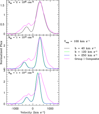
Figure 12.— Emergent Ly$\alpha$ profiles from simple shell models that are qualitatively similar to Group I spectra. All panels show the predicted profiles for a central monochromatic source passing through an expanding shell with $V_{\rm exp}=$100 km s^-1. The top panel features a model with $N_{HI}=2\times 10^{20}\mbox{ cm}^{-2}$and Doppler parameter $b=40$ km s^-1. The middle and bottom panels show the results for models with $N_{HI}=1\times 10^{19}\mbox{ cm}^{-2}$ and $N_{HI}=1\times 10^{17}\mbox{ cm}^{-2}$, respectively. In both of these panels, the predicted profiles are shown for Doppler parameters $b=$ 120 and 250 km s^-1. In all panels, a double-peak profile is shown, with two peaks straddling the velocity field zeropoint, and a stronger red peak. Overplotted on each panel is the Group I continuum-subtracted composite spectrum. The Group I spectrum was normalized to match the primary peak height of each model. The $N_{HI}=2\times 10^{20}\mbox{ cm}^{-2}$ model has the closest resemblance to the typical properties of the Group I Ly$\alpha$ spectra in terms of both precise peak locations and line widths. The $N_{HI}=1\times 10^{17}\mbox{ cm}^{-2}$ model displays peaks that are both too close together in velocity space and too narrow. While the peak locations in the $N_{HI}=1\times 10^{19}\mbox{ cm}^{-2}$ model are a fine match to the Group I composite spectrum, the predicted line widths are still too narrow.

Like the spectra in Group II, Group III spectra also exhibit a stronger blue peak in the Ly$\alpha$ profile, but both blue and red peaks are redshifted relative to the velocity-field zeropoint, and most likely trace outflowing rather than inflowing gas. Only one of the two Group III objects (SSA22a-C49) has measurable low-ionization interstellar absorption. From these features, we measure a significant blueshift of $\Delta v\sim-230$ km s^-1, and a line width of $\sigma_{abs}\sim 230$ km s^-1. In terms of the simple shell models shown in Figure 11, the closest match to Group III is found for $V_{\rm exp}=400$ km s^-1, and $b=40$ km s^-1. As discussed by Yang et al. (2011), the blueshifted peak in a shell model decreases in strength as $V_{\rm exp}/b$ increases. This trend is reflected in the large $V_{\rm exp}/b$ model discussed here, with its lack of significant flux bluewards of zero, and two peaks redshifted relative to zero. Although there is qualitative agreement between the model and Group III spectra, in so far as both have two peaks redshifted relative to zero, and no significant flux bluewards of zero, the actual peak separations and locations in the model and data do not agree in detail. The model predicts $\Delta v_{peak}\sim 600$ km s^-1, while the Group III objects have $\Delta v_{peak}\sim 400$ km s^-1. Furthermore, the blue peak in the model is shifted by only $\sim+100$ km s^-1 relative to zero, while the blue peak in SSA22a-C49 is shifted by $>+500$ km s^-1 relative to zero. Finally, the relatively small Doppler parameter of $b=40$ km s^-1 would give rise to significantly narrower low-ionization interstellar absorption line widths than those observed. While Group III objects most likely indicate the presence of an outflow, the models described here still present some mismatches with the Group III data.

Distinguishing between Group II and Group III objects by establishing the velocity-field zeropoint has potentially important consequences. Over the last several years, the process of galaxy growth through cold gas accretion has received much attention in the theoretical literature. Both analytic calculations (Birnboim & Dekel, 2003) and numerical simulations (Fardal et al., 2001; Kereš et al., 2005, 2009; Dekel et al., 2009) suggest that high-redshift galaxies primarily grow by smoothly accreting cold gas from the surrounding IGM. Identifying observational signatures of infalling gas is crucial for testing the theoretical paradigm of cold accretion. In particular, since the predicted signatures of accreting gas in low-ionization metal absorption lines are so weak, due to the low metallicity of infalling material (Fumagalli et al., 2011), the Ly$\alpha$ feature may represent the best hope for detecting cosmological infall. Beyond the Group II and Group III objects in our NIRSPEC sample, $\sim 30$% of the double-peaked spectra in the LRIS parent sample have a stronger blue peak. If the velocity-field zeropoint can be established in these objects, to test whether the stronger blue peak is also blueshifted relative to zero (i.e., distinguishing between Group II and Group III spectra), their Ly$\alpha$ spectra may provide evidence for and constraints on the nature of gas infall in star-forming galaxies at $z\sim 2-3$.

For the remaining three spectra (Groups IV and V), we do not find even qualitative matches among the simple models presented here. Indeed, for SSA22a-D17 and SSA22a-C31 (Group IV), there are two peaks with roughly equal heights, as seen in a static configuration. However, the locations of the peaks are not symmetrically distributed around the velocity-field zeropoint, as would be expected for a static shell, and the interpeak trough is redshifted by several hundred km s^-1. Furthermore, SSA22a-D17 has an extremely large low-ionization interstellar absorption blueshift measured, with $\Delta v\sim-1170$ km s^-1, which additionally rules out the static case. Q1623-BX129 has two strong peaks with roughly equal heights and similar locations to those of SSA22a-D17 and SSA22a-C31, plus a third, redder peak, which is significantly weaker. A larger model parameter space will be required to match the profile shapes of these three objects.

In summary, while general qualitative matches can be found for the Group I, Group II, and Group III Ly$\alpha$ profile types, we find notable specific discrepancies between the models and the totality of the data presented here – with particular attention to the interstellar absorption profiles. One important issue is that the shell models that provide the best matches to, e.g., Group I profiles ($V_{\rm exp}=100$ km s^-1, $b=40$ km s^-1), are not able to match simultaneously the broad low-ionization interstellar absorption troughs characterized by a median of $\sigma_{abs,med}\sim 190$ km s^-1. We also highlight the importance of our new NIRSPEC measurements for untangling the nature of these Ly$\alpha$ spectra. Measurements of the velocity-field zeropoint (i.e. from the H$\alpha$ or [OIII] redshift) are key for distinguishing between Group II (inflow) and Group III (strong outflow) objects. Furthermore, determining the velocity width of the input Ly$\alpha$ spectrum (based on the H$\alpha$ or [OIII] velocity dispersion), so that it is not a free parameter of Ly$\alpha$ radiative transfer models, reduces the degeneracies associated with fitting physical models to Ly$\alpha$ profiles. Indeed, when fitting the double-peaked Ly$\alpha$ profile for an object with unconstrained systemic velocity and input Ly$\alpha$ velocity dispersion, Verhamme et al. (2008) find two expanding-shell model solutions that differ by 5 orders of magnitude in inferred hydrogen column density (see their Figure 8). One of the best-fit models has an inferred intrinsic Ly$\alpha$ FWHM$=700$ km s^-1 – a factor of three larger than the average for our sample! Furthermore, the placement of the velocity-field zeropoint differs by $\sim 500$ km s^-1 for the two best-fit models in question. Verhamme et al. (2008) conclude that neither solution is satisfactory and that future observations are needed to constrain their models. With systemic redshift and velocity dispersion measurements, such degeneracy in best-fit models is no longer allowed, potentially leading to much tighter constraints on the underlying physical picture.

6.3. Additional Considerations and Caveats

In the preceding discussion, within the framework of expanding/infalling shell models, we presented an interpretation of the observed low-ionization interstellar absorption line widths in terms of the random thermal broadening of gas in the shell. An alternative explanation of interstellar absorption line widths is presented in Steidel et al. (2010), according to which absorption is produced by a population of discreet clouds at a large range of galactocentric radii (i.e., not a thin shell). The expansion velocities of these clouds increase smoothly and monotonically with increasing radius, and their covering fraction is a decreasing function of radius. In such a model, in which photons scatter off of the $\tau_{Ly\alpha}=1$ surfaces of discrete clouds, the nature of the bulk gas kinematics modulates the emergent Ly$\alpha$ profiles, as opposed to the neutral hydrogen column density and Doppler $b$-parameter of individual clouds. This clumpy outflow model accounts for the typical interstellar absorption profiles both along the line of sight to individual UV-selected star-forming galaxies at $z\sim 2-3$, as well as along averaged offset sightlines with impact parameters up to $\sim 100$ physical kpc, and predicts extended Ly$\alpha$ emission consistent with the observations (Steidel et al., 2011). At the same time, high-resolution 3D cosmological hydrodynamical simulations that follow the radiative transfer of Ly$\alpha$ photons through the gas distributions surrounding high-redshift galaxies are highlighting the importance of orientation effects. The gas column density and velocity distributions in these simulated galaxies are anisotropic and irregular, characterized by clumps and filaments of infalling and outflowing cold gas (Laursen et al., 2009a; Barnes et al., 2011). This anisotropy leads to a strong dependence of the shape of the emergent Ly$\alpha$ profile on viewing angle. For example, if the line of sight to a galaxy intercepts a filament of infalling gas, a blue-asymmetric peak may be observed, even in the presence of outflowing gas in the system (Barnes et al., 2011). A close comparison is required between the predictions of such simulations and the full ensemble of Ly$\alpha$ profiles observed in LBGs, as well as incorporating detailed Ly$\alpha$ radiative transfer calculations from Zheng & Miralda-Escudé (2002) and Kollmeier et al. (2010) into the clumpy outflow model of Steidel et al. (2010).

Another potentially important effect to consider is absorption by the IGM (Dijkstra et al., 2007; Zheng et al., 2010). Recent simulations by Laursen et al. (2011) have demonstrated that the blue peak in an emergent double-peaked Ly$\alpha$ profile may be suppressed due to absorption by neutral hydrogen external to a galaxy. For the purposes of such analysis, “IGM” is defined as gas located at a radius greater than $\sim 1.5$ times the dark-matter halo virial radius. IGM absorption may be significant even at redshifts well below the epoch of reionization. This result is relevant to the interpretation of our Group I profile types. In such objects, the Ly$\alpha$ peak bluewards of the systemic velocity is weaker than the red peak. We have compared these profiles to simple galactic-scale models for outflowing gas, in which the asymmetry arises due to the radiative transfer of Ly$\alpha$ photons, and have ignored the possible effects of IGM absorption on the observed red-to-blue peak ratio. One simple test for the importance of IGM absorption consists of examining the distribution of red-to-blue peak ratios as a function of redshift within the LRIS double-peaked parent sample. For this test, we divide the sample into high- ($z\sim 3$) and low-redshift ($z\sim 2$) subsamples at a threshold redshift of $z=2.7$, and calculate the median red-to-blue peak ratio for each subsample. If IGM effects are significant, we expect to see the red-to-blue peak ratio evolve towards lower values at lower redshifts, as the blue peak becomes less suppressed by IGM absorption (under the assumption that the two samples have the same intrinsic distributions of double-peaked Ly$\alpha$ profile shapes before being subject to IGM absorption). In fact, we find that the median red-to-blue peak flux ratios for $z\sim 3$ and $z\sim 2$ subsamples are 1.3 and 1.5, respectively, and not statistically distinguishable. Therefore, IGM absorption does not appear to have a significant impact on the observed multiple-peaked Ly$\alpha$ profile shapes in our sample.

Finally, we must admit the possibility of an entirely different explanation for the origin of multiple-peaked Ly$\alpha$ emission profiles, such as galaxy mergers. A multiple-peaked profile would naturally result from a system in a merger state, with different peaks corresponding to different merging components (Cooke et al., 2010; Rauch et al., 2011). The continuum and emission-line morphology of objects in our sample are crucial to consider when examining possible merger models. Figure 1 shows the (seeing-limited) $\cal R$-band morphologies for objects in our sample. The majority of our targets appear to be consistent with single components at this resolution. A small number of objects, however, are slightly extended (e.g. Q2206-BX151, Q1549-M22) or appear to have multiple components (e.g. Q0449-BX167, Westphal-BX154). Three of these objects have already been discussed in Section 3.1.1 in terms of their complex two-dimensional spectra. If our multiple-peaked Ly$\alpha$ profiles were simply caused by mergers, there should be evidence of multiple-peaked emission in the rest-frame optical nebular lines (i.e., H$\alpha$ and [OIII]). These features more closely trace the systemic velocity and dynamics and are typically not as sensitive to bulk outflow motions as the Ly$\alpha$ emission line. As described in Section 3.1.1, only Q1549-M22 shows possible signs of nebular lines with multiple-peaked behavior in the spectral direction, ruling out mergers as a possible explanation for the majority of our Ly$\alpha$ profiles.

7. Summary and Discussion

There is strong observational evidence for the ubiquity of large-scale outflows in high-redshift star-forming galaxies. Gauging the overall impact of these large-scale outflows on the evolution of the galaxies sustaining them remains an open challenge. Theoretical considerations suggest that, at the same cosmic epochs, the inflow of cold gas is also a very important process in the evolution of star-forming galaxies. Multiple-peaked Ly$\alpha$ profiles in star-forming UV-selected galaxies at $z\sim 2-3$ offer a unique probe of both outflows and inflows in the early universe. The complex line structure potentially provides constraints on many important gas flow parameters. Specifically, the locations of peaks with respect to the velocity-field zeropoint, their separations, and flux ratios are all additional pieces of information not seen in single-peaked Ly$\alpha$ profiles. Along with observational data such as accurate systemic redshifts, intrinsic nebular line widths, and intrinsic ionizing photon fluxes, one can distinguish among the possible processes underlying these systems.

We have shown that the phenomenon of multiple-peaked profiles appears in a significant fraction ($\sim$ 30$\%$) of UV-selected star-forming galaxies at $z\sim 2-3$ with Ly$\alpha$ emission. After identifying possible candidates for this study we presented a sample of 18 multiple-peaked objects with observed H$\alpha$ or [OIII] nebular emission lines, which were used to establish accurate systemic redshift measurements. The average velocity dispersion, $\sigma_{v}$, and the mean star-formation rate in our sample are comparable to values measured from the full population of UV-selected star-forming galaxies at $z\sim 2-3$. At the same time, given our focus on Ly$\alpha$-emitting galaxies, the average $E(B-V)$ in our sample is bluer than what is typically measured. Detected interstellar absorption lines for objects in the sample show, on average, a blueshift, which is suggestive of large-scale outflows driven by supernovae or winds of massive stars. Additionally, the interstellar absorption line widths are measured to be $\langle\sigma_{abs}\rangle\sim 200$ km s^-1, which is similar to values found in other studies of star-forming galaxies at $z\sim 2-3$. A comparison of our interstellar absorption line widths to a sample of star-forming galaxies with single-peaked Ly$\alpha$ emission show the single-peaked objects to have consistently larger interstellar absorption line widths. The difference in interstellar absorption line widths may signify that the ranges of gas velocities are different for multiple-peaked compared to single-peaked Ly$\alpha$ emission objects.

We have qualitatively compared our observed Ly$\alpha$ profiles with simple models of expanding and infalling gaseous shells and halos, given the attention such models have recently received in the literature (Verhamme et al., 2006, 2008; Schaerer & Verhamme, 2008). The closest match between these simple models and our data is found for Group I type profiles, which make up 11 out of 18 of the NIRSPEC sample objects, and are characterized by a red-asymmetric double peak straddling the velocity-field zeropoint. Group I type profiles can be produced in an expanding shell model, with a high-column density ($N=2\times 10^{20}\mbox{ cm}^{-2}$), moderate expansion speed ($V_{\rm exp}=100$ km s^-1), and small Doppler parameter, ($b=40$ km s^-1). At the same time, the observed low-ionization interstellar absorption line profiles for Group I objects are significantly broader than the features that would arise from an expanding shell with $b=40$ km s^-1, and signal a problem with the above interpretation for the Group I Ly$\alpha$ spectra. Certain aspects of Group II and Group III Ly$\alpha$ spectra are also reproduced by the simple models considered here, though, in detail, the matches are not perfect. For the remaining handful of objects in our NIRSPEC multiple-peaked sample, the suite of models we’ve considered cannot be used to explain the observed profiles, both in terms of Ly$\alpha$ peak locations, relative strengths, and numbers.

It is also of interest to compare Ly$\alpha$ radiative transfer models with high-redshift data of significantly higher S/N and resolution than the spectra presented here. Quider et al. (2009) present the multiple-peaked Ly$\alpha$ emission profile of the strongly gravitationally lensed galaxy, “the Cosmic Horseshoe,” for which the magnification is estimated to be a factor of $\sim 24$. The Cosmic Horseshoe has a very well-defined stellar systemic redshift, from which the Ly$\alpha$ spectral profile can be calculated in velocity space. While an expanding shell model from Verhamme et al. (2006) with $N_{HI}=7\times 10^{19}\mbox{ cm}^{-2}$, $V_{\rm exp}=300$ km s^-1, and $b=40$ km s^-1, provides a qualitative match to the two redshifted peaks in the Cosmic Horseshoe Ly$\alpha$ profile, the small Doppler $b$-parameter in the model is again at odds with the broad low-ionization interstellar absorption profile. Furthermore, in detail, the locations of the Ly$\alpha$ peaks in the predicted model spectrum do not line up with those of the observations. Both typical and strongly-lensed UV-selected star-forming galaxies with well-determined systemic redshifts and, accordingly, Ly$\alpha$ profiles calculated robustly in velocity space are now providing important observational constraints on Ly$\alpha$ radiative transfer models. These objects highlight the need for considering simultaneously the emergent Ly$\alpha$ emission profile, and the profile of low-ionization interstellar absorption, which must be matched within a unified framework (Steidel et al., 2010).

While we have mainly focused here on the discrepancies between models and data, and have therefore not yet been able to derive the physical parameters of the gaseous flows surrounding UV-selected star-forming galaxies at high redshift, we view this analysis as an important initial step. It will simply not be possible to constrain the gas density and velocity distributions in these circumgalactic flows without the simultaneous establishment of the location of the multiple-peaked Ly$\alpha$ profile and interstellar absorption features in velocity space. We have presented such measurements here for a sample of objects whose red- and blue-asymmetric multiple-peaked Ly$\alpha$ profiles at least qualitatively suggest a range of processes including both outflows and infall. Additional critical observables presented here which will be be considered in future modeling are the input velocity distribution of Ly$\alpha$ photons as traced by the velocity dispersion of either H$\alpha$ or [OIII] emission, and the degree of dust attenuation as traced by rest-frame UV colors and Ly$\alpha$/H$\alpha$ flux ratios. With a realistic model that successfully matches the combination of intrinsic and emergent Ly$\alpha$ velocity distributions as well as interstellar absorption profiles, we will obtain the gas density and velocity distribution as a function of radius. These distributions will potentially allow us to constrain the rates at which cold gas mass is flowing in and out of galaxies, which represents one of the most important goals in the study of galaxy formation.

References

- Adelberger et al. (2005) Adelberger, K. L., Steidel, C. C., Pettini, M., Shapley, A. E., Reddy, N. A., & Erb, D. K. 2005, ApJ, 619, 697
- Adelberger et al. (2003) Adelberger, K. L., Steidel, C. C., Shapley, A. E., & Pettini, M. 2003, ApJ, 584, 45
- Ahn et al. (2002) Ahn, S., Lee, H., & Lee, H. M. 2002, ApJ, 567, 922
- Barnes et al. (2011) Barnes, L. A., Haehnelt, M. G., Tescari, E., & Viel, M. 2011, ArXiv e-prints
- Birnboim & Dekel (2003) Birnboim, Y. & Dekel, A. 2003, MNRAS, 345, 349
- Bruzual & Charlot (2003) Bruzual, G. & Charlot, S. 2003, MNRAS, 344, 1000
- Calzetti et al. (2000) Calzetti, D., Armus, L., Bohlin, R. C., Kinney, A. L., Koornneef, J., & Storchi-Bergmann, T. 2000, ApJ, 533, 682
- Chabrier (2003) Chabrier, G. 2003, PASP, 115, 763
- Cooke et al. (2010) Cooke, J., Berrier, J. C., Barton, E. J., Bullock, J. S., & Wolfe, A. M. 2010, MNRAS, 403, 1020
- Dekel et al. (2009) Dekel, A., Birnboim, Y., Engel, G., Freundlich, J., Goerdt, T., Mumcuoglu, M., Neistein, E., Pichon, C., Teyssier, R., & Zinger, E. 2009, Nature, 457, 451
- Dijkstra et al. (2006) Dijkstra, M., Haiman, Z., & Spaans, M. 2006, ApJ, 649, 14
- Dijkstra et al. (2007) Dijkstra, M., Lidz, A., & Wyithe, J. S. B. 2007, MNRAS, 377, 1175
- Erb et al. (2003) Erb, D. K., Shapley, A. E., Steidel, C. C., Pettini, M., Adelberger, K. L., Hunt, M. P., Moorwood, A. F. M., & Cuby, J. 2003, ApJ, 591, 101
- Erb et al. (2006a) Erb, D. K., Steidel, C. C., Shapley, A. E., Pettini, M., Reddy, N. A., & Adelberger, K. L. 2006a, ApJ, 647, 128
- Erb et al. (2006b) —. 2006b, ApJ, 646, 107
- Fardal et al. (2001) Fardal, M. A., Katz, N., Gardner, J. P., Hernquist, L., Weinberg, D. H., & Davé, R. 2001, ApJ, 562, 605
- Fumagalli et al. (2011) Fumagalli, M., Prochaska, J. X., Kasen, D., Dekel, A., Ceverino, D., & Primack, J. R. 2011, ArXiv e-prints
- Hansen & Oh (2006) Hansen, M. & Oh, S. P. 2006, MNRAS, 367, 979
- Kelson (2003) Kelson, D. D. 2003, PASP, 115, 688
- Kennicutt (1998a) Kennicutt, Jr., R. C. 1998a, ARA&A, 36, 189
- Kennicutt (1998b) —. 1998b, ApJ, 498, 541
- Kereš et al. (2009) Kereš, D., Katz, N., Fardal, M., Davé, R., & Weinberg, D. H. 2009, MNRAS, 395, 160
- Kereš et al. (2005) Kereš, D., Katz, N., Weinberg, D. H., & Davé, R. 2005, MNRAS, 363, 2
- Kollmeier et al. (2010) Kollmeier, J. A., Zheng, Z., Davé, R., Gould, A., Katz, N., Miralda-Escudé, J., & Weinberg, D. H. 2010, ApJ, 708, 1048
- Kornei et al. (2010) Kornei, K. A., Shapley, A. E., Erb, D. K., Steidel, C. C., Reddy, N. A., Pettini, M., & Bogosavljević, M. 2010, ApJ, 711, 693
- Laursen et al. (2009a) Laursen, P., Razoumov, A. O., & Sommer-Larsen, J. 2009a, ApJ, 696, 853
- Laursen et al. (2009b) Laursen, P., Sommer-Larsen, J., & Andersen, A. C. 2009b, ApJ, 704, 1640
- Laursen et al. (2011) Laursen, P., Sommer-Larsen, J., & Razoumov, A. O. 2011, ApJ, 728, 52
- Liu et al. (2008) Liu, X., Shapley, A. E., Coil, A. L., Brinchmann, J., & Ma, C. 2008, ApJ, 678, 758
- Madau (1995) Madau, P. 1995, ApJ, 441, 18
- McLean et al. (1998) McLean, I. S., Becklin, E. E., Bendiksen, O., Brims, G., Canfield, J., Figer, D. F., Graham, J. R., Hare, J., Lacayanga, F., Larkin, J. E., Larson, S. B., Levenson, N., Magnone, N., Teplitz, H., & Wong, W. 1998, in Society of Photo-Optical Instrumentation Engineers (SPIE) Conference Series, Vol. 3354, Society of Photo-Optical Instrumentation Engineers (SPIE) Conference Series, ed. A. M. Fowler, 566–578
- McLinden et al. (2011) McLinden, E. M., Finkelstein, S. L., Rhoads, J. E., Malhotra, S., Hibon, P., Richardson, M. L. A., Cresci, G., Quirrenbach, A., Pasquali, A., Bian, F., Fan, X., & Woodward, C. E. 2011, ApJ, 730, 136
- Oke et al. (1995) Oke, J. B., Cohen, J. G., Carr, M., Cromer, J., Dingizian, A., Harris, F. H., Labrecque, S., Lucinio, R., Schaal, W., Epps, H., & Miller, J. 1995, PASP, 107, 375
- Osterbrock (1962) Osterbrock, D. E. 1962, ApJ, 135, 195
- Osterbrock (1989) —. 1989, Astrophysics of gaseous nebulae and active galactic nuclei
- Pettini et al. (2001) Pettini, M., Shapley, A. E., Steidel, C. C., Cuby, J., Dickinson, M., Moorwood, A. F. M., Adelberger, K. L., & Giavalisco, M. 2001, ApJ, 554, 981
- Quider et al. (2009) Quider, A. M., Pettini, M., Shapley, A. E., & Steidel, C. C. 2009, MNRAS, 398, 1263
- Rauch et al. (2011) Rauch, M., Becker, G. D., Haehnelt, M. G., Gauthier, J.-R., Ravindranath, S., & Sargent, W. L. W. 2011, ArXiv e-prints
- Reddy et al. (2008) Reddy, N. A., Steidel, C. C., Pettini, M., Adelberger, K. L., Shapley, A. E., Erb, D. K., & Dickinson, M. 2008, ApJS, 175, 48
- Schaerer & Verhamme (2008) Schaerer, D. & Verhamme, A. 2008, A&A, 480, 369
- Shapley et al. (2005) Shapley, A. E., Coil, A. L., Ma, C., & Bundy, K. 2005, ApJ, 635, 1006
- Shapley et al. (2003) Shapley, A. E., Steidel, C. C., Pettini, M., & Adelberger, K. L. 2003, ApJ, 588, 65
- Steidel et al. (2003) Steidel, C. C., Adelberger, K. L., Shapley, A. E., Pettini, M., Dickinson, M., & Giavalisco, M. 2003, ApJ, 592, 728
- Steidel et al. (2011) Steidel, C. C., Bogosavljević, M., Shapley, A. E., Kollmeier, J. A., Reddy, N. A., Erb, D. K., & Pettini, M. 2011, ArXiv e-prints
- Steidel et al. (2010) Steidel, C. C., Erb, D. K., Shapley, A. E., Pettini, M., Reddy, N., Bogosavljević, M., Rudie, G. C., & Rakic, O. 2010, ApJ, 717, 289
- Steidel et al. (2004) Steidel, C. C., Shapley, A. E., Pettini, M., Adelberger, K. L., Erb, D. K., Reddy, N. A., & Hunt, M. P. 2004, ApJ, 604, 534
- Tapken et al. (2007) Tapken, C., Appenzeller, I., Noll, S., Richling, S., Heidt, J., Meinköhn, E., & Mehlert, D. 2007, A&A, 467, 63
- Veilleux et al. (2005) Veilleux, S., Cecil, G., & Bland-Hawthorn, J. 2005, ARA&A, 43, 769
- Verhamme et al. (2008) Verhamme, A., Schaerer, D., Atek, H., & Tapken, C. 2008, A&A, 491, 89
- Verhamme et al. (2006) Verhamme, A., Schaerer, D., & Maselli, A. 2006, A&A, 460, 397
- Yang et al. (2011) Yang, Y., Zabludoff, A., Jahnke, K., Eisenstein, D., Davé, R., Shectman, S. A., & Kelson, D. D. 2011, ApJ, 735, 87
- Zheng et al. (2010) Zheng, Z., Cen, R., Trac, H., & Miralda-Escudé, J. 2010, ApJ, 716, 574
- Zheng & Miralda-Escudé (2002) Zheng, Z. & Miralda-Escudé, J. 2002, ApJ, 578, 33