IPMU11-0119

Higher Derivative Corrections to Holographic Entanglement Entropy
for AdS Solitons
Noriaki Ogawa and Tadashi Takayanagi
Institute for the Physics and Mathematics of the Universe (IPMU),
University of Tokyo, Kashiwa, Chiba 277-8582, Japan

We investigate the behaviors of holographic entanglement entropy for AdS soliton geometries in the presence of higher derivative corrections. We calculate the leading higher derivative corrections for the AdS₅ setup in type IIB string and for the AdS_4,7 ones in M-theory. We also study the holographic entanglement entropy in Gauss-Bonnet gravity and study how the confinement/deconfinement phase transition observed in AdS solitons is affected by the higher derivative corrections.

1 Introduction

The entanglement entropy is a useful universal quantity when we would like to employ the AdS/CFT correspondence [2] to study non-perturbative aspects of string theory as quantum gravity. In [3], it has been proposed that the entanglement entropy in conformal field theories (CFTs) can be calculated from the area of minimal surface in anti de-Sitter (AdS) spaces. It is explicitly given by the formula

$$S_{A}=\frac{\mbox{Area}(\gamma_{A})}{4G_{N}},$$ (1)

where $G_{N}$ is the Newton constant in the Einstein gravity on the AdS space; $S_{A}$ is the entanglement entropy for the subsystem $A$, which can be chosen arbitrarily; $\gamma_{A}$ is the codimension two minimal area surface which ends on the boundary of $A$. Also we require $\gamma_{A}$ is homologous to $A$. Even though there has been no precise proof of this formula (1), many non-trivial evidences have been accumulated until now. For example, the strong subadditivity, which is one of the most important inequality satisfied by the entanglement entropy, has been shown in [4]. Quite recently, the paper [5] showed that all known inequalities are satisfied by the holographic entanglement entropy (HEE) given by (1) and moreover HEE leads to more constrained inequalities than entanglement entropies in general quantum field theories. Also, the agreements of the logarithmic terms in both side has been shown in [3, 6, 7, 8, 10, 9, 11]. Moreover, in [12], a highly non-trivial consistency check has been made when the subsystem $A$ is two intervals [13] in two dimensional CFTs by employing so called Renyi entropies. Refer to [14] and references therein for more evidences. For quantum field theoretic analysis of entanglement entropy refer e.g. to the excellent reviews [15, 16].

The holographic entanglement entropy (1) assumes that the gravity on the AdS space is defined by the Einstein gravity with a negative cosmological constant. In the CFT side, this means that we are taking the large ’t Hooft coupling limit. To analyze a full quantum gravity which appears in string theory and to extend the results to the weak coupling region of the CFT dual, we need to include quantum corrections which are effectively described by higher derivative terms. In the recent papers [17, 18] studied the corrections of holographic entanglement entropy in the presence of higher derivative terms (see also [19] for related discussions). Though it is very complicated to find a holographic entanglement entropy formula for general higher derivative corrections as noted in [17], a class of theories called Lovelock gravities, the authors of [17, 18] found important evidences that natural extensions of (1) give the correct holographic entanglement entropy. In the ${\mathcal{R}}^{2}$ Gauss-Bonnet gravity, which is the simplest example of Lovelock gravities, it is given by the following formula (this expression itself has been already speculated in [20])

$$S_{A}=\frac{1}{4G_{N}}\int_{\gamma_{A}}\sqrt{h}(1+\eta L^{2}{\mathcal{R}}),$$ (2)

where $\eta$ is the coupling constant of Gauss-Bonnet term, which will be explained later; $h$ is the induced metric on the three dimensional surface $\gamma_{A}$ chosen arbitrarily; ${\mathcal{R}}$ is the intrinsic curvature of $h$. We again require that $\gamma_{A}$ has a boundary which coincides with that of $A$ and we need to add a boundary Gibbons-Hawking term to (2) in actual calculations. The profile of $\gamma_{A}$ is determined by minimizing the functional (2).

The purpose of this paper is to investigate further the properties of higher derivative corrections of the entanglement entropy. In the first half of this paper, we will consider explicit setups of string/M-theory and calculate the higher derivative corrections of the holographic entanglement entropy. Since the leading higher derivative correction is the quartic polynomial of the Weyl curvature [21, 22], this is not in the class of Lovelock gravities. To obtain non-trivial results in a tractable way, we will concentrate on the examples of AdS soliton spaces, which are dual to confining gauge theories [23], and choose the subsystem as just the half of the total space. In the type IIB string case, this is dual to the subleading corrections to the entanglement entropy in the ${\mathcal{N}}=4$ super Yang-Mills (SYM) on a circle with the anti-periodic boundary condition for fermions. In the latter half of this paper, we will study the holographic entanglement entropy in the 4D and 5D Gauss-Bonnet gravity, especially when the subsystem $A$ is defined by a strip. We will analyze the behavior of the entropy when we change the width of the strip and see how the phase transition is affected by the higher derivatives. The holographic entanglement entropy for AdS solitons without higher derivative corrections has been already studied in [24, 25, 26]. Later, qualitatively similar results has been recently reproduced in lattice gauge theory approaches [27, 28, 29].

This paper is organized as follows: In section 2 we calculate the higher derivative corrections of holographic entanglement entropy for the AdS₅ soliton in IIB string and for the AdS_4,7 soliton in M-theory. In section 3, we compute the holographic entanglement entropy for AdS soliton in the Gauss-Bonnet gravity in four and five dimension. We choose the subsystem $A$ to be a half space in all of the above calculations. In section 4, we analyze the holographic entanglement entropy for AdS soliton in the five dimensional Gauss-Bonnet gravity when $A$ is give by a strip. In section 5, we summarize our conclusions.

2 Holographic Entanglement Entropy with Higher Derivative Corrections in String and M Theories

In this section, we will investigate the leading higher derivative corrections to the holographic entanglement entropy in string theory and M-theory. We consider AdS₅ soliton geometry in type IIB superstring and AdS₄ and AdS₇ soliton geometries in M-theory. We choose the subsystem A as the half of the total space.

2.1 Type IIB Superstring

Consider the AdS${}_{5}\times$S⁵ solution in type IIB string theory. The relevant part of the type IIB supergravity action with the leading $\alpha^{\prime}$ correction looks like in the Euclidean signature [21]

$$I=-\frac{1}{16\pi G^{(10)}_{N}}\int dx^{10}\sqrt{g}\left[{\mathcal{R}}-\frac{1}{2}(\partial_{\mu}\phi)^{2}-\frac{1}{4\cdot 5\!}F_{5}^{2}+\dotsc+\gamma\cdot e^{-\frac{3}{2}\phi}W+\dotsc\right],$$ (3)

where we keep the relevant terms which are linear with respect to $\gamma$, which is supposed to be very small. There are also other such terms depending on other antisymmetric fields, represented by dots, but they do not have any contributions to our discussions below. $W$ is defined by the following ${\mathcal{R}}^{4}$ term by using the Weyl curvature ${\mathcal{C}}$

$$W={\mathcal{C}}^{hmnk}{\mathcal{C}}_{pmnq}{\mathcal{C}}_{h}^{\ rsp}{\mathcal{C}}^{q}_{\ rsk}+\frac{1}{2}{\mathcal{C}}^{hkmn}{\mathcal{C}}_{pqmn}{\mathcal{C}}_{h}^{\ rsp}{\mathcal{C}}^{q}_{\ rsk},$$ (4)

and the constant $\gamma$ is give by

$$\gamma=\frac{1}{8}\zeta(3)\alpha^{\prime 3}.$$ (5)

The AdS${}_{5}\times$ S⁵ is the solution to this theory with the higher derivatives. This type IIB string background is dual to the four dimensional ${\mathcal{N}}=4$ $SU(N)$ super Yang-Mills theory [2]. The standard dictionary tells us that the AdS radius $L$ is related to the ’t Hooft coupling $\lambda=2\pi g_{s}N$ by

$$L^{4}=4\pi g_{s}\alpha^{\prime 2}N=2\lambda\alpha^{\prime 2}.$$ (6)

Therefore taking into account the linear order of $\gamma$ is to consider the next leading order correction in the strong coupling expansion of $\lambda$. The Yang-Mills coupling is related to the string coupling

$$g^{2}_{YM}=2\pi g_{s}.$$ (7)

The ten dimensional Newton constant is given by

$$G^{(10)}_{N}=8\pi^{6}\alpha^{\prime 4}g_{s}^{2}=\frac{\pi^{4}L^{8}}{2N^{2}}.$$ (8)

2.1.1 AdS₅ soliton and the large ’t Hooft coupling limit of $\mathcal{N}=4$ SYM

Consider the AdS₅ soliton background, which is dual to the ${\mathcal{N}}=4$ SYM compactified on a circle $S^{1}$ (radius $R$) with the anti-periodic boundary condition for fermions [23]. Its leading order solution (i.e. $\gamma=0$) is given by

$$ds^{2}=\frac{r^{2}}{L^{2}}[dt_{E}^{2}+dx^{2}+dy^{2}]+\frac{L^{2}}{r^{2}}\frac{dr^{2}}{1-r^{4}_{0}/r^{4}}+\frac{r^{2}}{L^{2}}(1-r_{0}^{4}/r^{4})d\theta^{2}+L^{2}d\Omega^{2}_{5}.$$ (9)

The periodicity of $\theta$ is given by $\theta\sim\theta+2\pi R$ with

$$R=\frac{L^{2}}{2r_{0}}.$$ (10)

We define the subsystem $A$ by the following half space on the time slice $t_{E}=0$

$$x>0,\ \ \ -\infty<y<\infty,\ \ \ 0\leq\theta<2\pi R.$$ (11)

The contribution of holographic entanglement entropy in the leading order of $\gamma$ is given by the area law formula (1). In the AdS soliton case, we obtain explicitly [24]

$$S^{(0)}_{A} = \frac{\mbox{Area}(\gamma_{A}^{(5)})}{4G^{(5)}_{N}}=\frac{\pi^{3}L^{4}}{8G^{10}_{N}}\frac{\pi L^{2}}{r_{0}}(r^{2}_{\infty}-r^{2}_{0})V_{1},$$ (12)

$$= \frac{N^{2}}{4L^{2}}\cdot\frac{r^{2}_{\infty}}{r_{0}}V_{1}-\frac{N^{2}V_{1}}{8R},$$

where we employed

$$G^{(5)}_{N}=\frac{G^{(10)}_{N}}{\mbox{vol}(S^{5})}=\frac{\pi L^{3}}{2N^{2}},$$ (13)

using $\mbox{vol}(S^{5})=\pi^{3}L^{5}$.

2.1.2 Higher derivative corrections to the entanglement entropy

Next we would like to calculate the higher derivative corrections to the previous calculation (12). To calculate the holographic entanglement entropy, we place a deficit angle $\delta=2\pi(1-n)$ on the three dimensional surface $\gamma_{A}$ defined by $x=t_{E}=0$ [30, 20, 3]. When the extrinsic curvature of the submanifold $\gamma_{A}$ is vanishing, the curvature tensor behaves like (assuming $1-n$ is infinitesimally small) [31]

$${\mathcal{R}}_{\mu\nu\rho\sigma}={\mathcal{R}}^{(0)}_{\mu\nu\rho\sigma}+2\pi(1-n)(N_{\mu\rho}N_{\nu\sigma}-N_{\mu\sigma}N_{\nu\rho})\delta(\gamma_{A}),$$

$${\mathcal{R}}_{\mu\nu}={\mathcal{R}}^{(0)}_{\mu\nu}+2\pi(1-n)N_{\mu\nu}\delta(\gamma_{A}),$$

$${\mathcal{R}}={\mathcal{R}}^{(0)}+4\pi(1-n)\delta(\gamma_{A}),$$ (14)

where we defined $N_{\mu\nu}=n^{t_{E}}_{\mu}n^{t_{E}}_{\nu}+n^{x}_{\mu}n^{x}_{\nu}$. The unit vectors $n^{t_{E}}_{\mu}$ and $n^{x}_{\mu}$ are orthogonal to the surface $\gamma_{A}$. ${\mathcal{R}}^{(0)}_{\mu\nu}$ etc. denotes the original curvature tensor without the deficit angle.

By plugging (14) into (4), we obtain

$$W=\frac{180r_{0}^{16}}{L^{8}r^{16}}+2\pi(n-1)\delta(\gamma_{A})\cdot\frac{40r^{12}_{0}}{L^{6}r^{12}}+O(\gamma)+O\left((1-n)^{2}\right).$$ (15)

Therefore, the contribution from the $W$-term is estimated to be

$$S^{(W)}_{A} = -\frac{\partial}{\partial n}\log\left.\frac{Z_{n}^{(W)}}{\left(Z_{1}^{(W)}\right)^{n}}\right|_{n=1}$$ (16)

$$= -\frac{\gamma}{16\pi G^{(10)}_{N}}\int_{\gamma_{A}}dx^{8}\sqrt{g_{\gamma_{A}}}\left[\frac{80\pi r^{12}_{0}}{L^{6}r^{12}}\right]$$

$$= -\frac{5\gamma r^{12}_{0}}{L^{7}G^{(5)}_{N}}(2\pi RV_{1})\int^{r_{\infty}}_{r_{0}}\frac{dr}{r^{11}}$$

$$= -\frac{\gamma N^{2}V_{1}}{2RL^{6}},$$

where $\sqrt{g_{\gamma_{A}}}=rL^{4}d\Omega_{5}$ is the induced volume factor on $\gamma_{A}$.

Next we need to consider the higher derivative corrections of the metric. It is given by

$$ds^{2}=e^{-\frac{10}{3}\nu}ds^{2}_{5}+e^{2\nu}(d\Omega_{5})^{2},$$ (17)

where $\nu$ is order $O(\gamma)$. The five dimensional part is given by a modification of the AdS soliton metric [32, 33]

$$ds^{2}=f(r)d\theta^{2}+\frac{1}{g(r)}dr^{2}+r^{2}(dt^{2}_{E}+dx^{2}+dy^{2}),$$ (18)

where

$$f(r)=\frac{r^{4}-r^{4}_{0}}{r^{2}}\left(1+\gamma\cdot\alpha(r)\right),$$

$$g(r)=\frac{r^{4}-r^{4}_{0}}{r^{2}}\left(1+\gamma\cdot\beta(r)\right).$$ (19)

The functions $\alpha(r)$ and $\beta(r)$ are defined by

$$\alpha(r)=-\frac{15}{L^{6}}\left(5\frac{r^{4}_{0}}{r^{4}}+5\frac{r^{8}_{0}}{r^{8}}-3\frac{r^{12}_{0}}{r^{12}}\right),$$

$$\beta(r)=-\frac{15}{L^{6}}\left(5\frac{r^{4}_{0}}{r^{4}}+5\frac{r^{8}_{0}}{r^{8}}-19\frac{r^{12}_{0}}{r^{12}}\right).$$ (20)

The radius in the $\theta$-direction can be found by requiring the smoothness of the metric

$$2\pi R=\frac{\pi L^{2}}{r_{0}}-\frac{15\pi\gamma}{r_{0}L^{4}}+O(\gamma^{2}).$$ (21)

Since we already took care of the $W$ term in (16), here we only consider the contribution from the Einstein-Hilbert term. This is simply given by the area law formula as

$$S^{(EH)}_{A} = \frac{V_{1}}{4G_{N}^{(5)}}\cdot\frac{2\pi R}{L}\cdot\left(\frac{r^{2}_{\infty}}{2}-\frac{r^{2}_{0}}{2}-12\gamma\frac{r^{2}_{0}}{L^{6}}\right)$$ (22)

$$= \frac{V_{1}N^{2}R}{2L^{4}}r^{2}_{\infty}-\frac{N^{2}V_{1}}{8R}+\frac{3\gamma N^{2}V_{1}}{4RL^{6}}+O(\gamma^{2}).$$

Finally the total expression of $S_{A}$ up to $O(\gamma)$ is given by

$$S_{A}=S^{(EH)}_{A}+S^{(W)}_{A} = \frac{V_{1}N^{2}R}{2L^{4}}r^{2}_{\infty}-\frac{N^{2}V_{1}}{8R}+\frac{\gamma N^{2}V_{1}}{4RL^{6}}$$ (23)

$$= (\mbox{div.})+\frac{N^{2}V_{1}}{R}\left(-\frac{1}{8}+\frac{\zeta(3)}{32}(2\lambda)^{-3/2}\right),$$

where div. denotes the quadratically divergent term. We are interested in its finite term, which is independent of the UV cut off. This final result means that the entropy increases as the ’t Hooft coupling gets decreased. Indeed, the free field theory result obtained in [24] is given by

$$S^{free}_{A}=(\mbox{div.})-\frac{N^{2}V_{1}}{12R},$$ (24)

and matches with this expectation from our gravity calculation.

2.2 M-Theory

It will be interesting to compute the higher derivative corrections of the holographic entanglement entropy in M-theory backgrounds. The one-loop corrected action of the 11D supergravity is given by [22]

$$I=-\frac{1}{2\kappa_{11}^{2}}\int dx^{11}\sqrt{g}\left[{\mathcal{R}}+\dotsc+\gamma\cdot W+\dotsc\right],$$ (25)

where the dots represent the terms depending on antisymmetric forms again. $W$ is given by the same form as (4), and $\gamma$ is

$$\gamma=\frac{4\pi^{2}}{3}\kappa_{11}^{\frac{4}{3}}.$$ (26)

The 11D Newtonian constant $G_{N}^{(11)}$ and the Planck length $\ell_{P}$ are related to $\kappa_{11}$ as

$$8\pi G_{N}^{(11)}=\kappa_{11}^{2}=2^{4}\pi^{5}\ell_{P}^{9}.$$ (27)

2.2.1 M2-brane Soliton

Consider the AdS₄ soliton which is dual to a three dimensional CFT on $N$ M2-branes compactified on a circle. First of all, upon dimensional reduction on an $S^{7}$, the correction term $I^{(W)}$ in (25) is reduced to

$$I^{(W)}=-\frac{1}{16\pi G_{N}^{(4)}}\int d^{4}x\sqrt{g_{4}}\,\gamma W_{4},$$ (28)

where $W_{4}$ is given by the same form as (4) in 4D and the 4D Newtonian constant $G_{N}^{(4)}$ is given by

$$G_{N}^{(4)}=\frac{G_{N}^{(11)}}{\mbox{vol}(S^{7})}.$$ (29)

Under this dimensional reduction, the one-loop corrected metric of the AdS₄ soliton geometry reads [34]

$$ds^{2}_{4}=f(r)d\theta^{2}+\frac{dr^{2}}{g(r)}+\frac{r^{2}}{L^{2}}(dt^{2}_{E}+dx^{2}),$$ (30)

where

$$f(r)=\frac{r^{2}}{L^{2}}\left(1-\frac{r^{3}_{0}}{r^{3}}\right)\cdot(1+\gamma\cdot\alpha(r)),$$

$$g(r)=\frac{r^{2}}{L^{2}}\left(1-\frac{r^{3}_{0}}{r^{3}}\right)\cdot(1+\gamma\cdot\beta(r)),$$

$$\alpha(r)=-\frac{1}{4L^{6}}\left(17\frac{r^{3}_{0}}{r^{3}}+17\frac{r^{6}_{0}}{r^{6}}-11\frac{r^{9}_{0}}{r^{9}}\right),$$

$$\beta(r)=-\frac{1}{4L^{6}}\left(17\frac{r^{3}_{0}}{r^{3}}+17\frac{r^{6}_{0}}{r^{6}}-67\frac{r^{9}_{0}}{r^{9}}\right).$$ (31)

The AdS radius $L$ is related to the number $N$ of M2-branes by

$$L^{9}=N^{3/2}\frac{\kappa^{2}_{11}}{2^{17/2}\cdot\pi^{5}},$$ (32)

and the volume of $S^{7}$ is given by

$$\mbox{Vol}(S^{7})=\frac{\pi^{4}}{3}(2L)^{7}.$$ (33)

The radius in the $\theta$-direction is found to be

$$2\pi R=\frac{4\pi L^{2}}{3r_{0}}-\frac{5\pi\gamma}{3L^{4}r_{0}}.$$ (34)

Using (26) (32), the expansion parameter $\gamma$ is reexpressed as

$$\gamma=\frac{2^{23/3}\cdot\pi^{16/3}}{3}\cdot\frac{L^{6}}{N}.$$ (35)

It is useful to note

$$\frac{\mbox{Vol}(S^{7})}{\kappa^{2}_{11}}=\frac{1}{2^{3/2}\cdot 3\pi}\cdot\frac{N^{3/2}}{L^{2}}.$$ (36)

In the presence of the deficit angle $\delta=2\pi(1-n)$, the higher derivative term $W_{4}$ behaves like

$$W_{4}=\frac{9}{2}\frac{r_{0}^{12}}{L^{8}r^{12}}+2\pi(1-n)\delta(\gamma_{A})\cdot\frac{6r_{0}^{9}}{L^{6}r^{9}}+O(\gamma)+O\left((1-n)^{2}\right),$$ (37)

using the uncorrected AdS₄ soliton metric. This leads to the contribution

$$S^{(W)}_{A}=\frac{3\pi^{2}\gamma Rr_{0}}{2\kappa^{2}_{11}L^{6}}\cdot\mbox{Vol}(S^{7}).$$ (38)

The contribution from the Einstein-Hilbert action can be found by applying the area formula to the corrected metric

$$S^{(EH)}_{A} = \frac{4\pi^{2}R}{\kappa^{2}_{11}}\cdot\mbox{Vol}(S^{7})\cdot\int^{r_{\infty}}_{r_{0}}dr\left(1-\frac{7\gamma}{L^{6}}\frac{r^{9}_{0}}{r^{9}}\right)$$ (39)

$$= \frac{4\pi^{2}R}{\kappa^{2}_{11}}\cdot\mbox{Vol}(S^{7})\cdot\left(r_{\infty}-\left(1+\frac{7\gamma}{8L^{6}}\right)r_{0}\right)$$

Finally the total contribution to $S_{A}$ is

$$S^{(EH)}+S^{(W)} = \frac{N^{3/2}}{L^{2}}\frac{1}{2^{3/2}\cdot 3\pi}\left(4\pi^{2}Rr_{\infty}-2\pi^{2}Rr_{0}\left(2+\frac{\gamma}{L^{6}}\right)\right)$$ (40)

$$= \frac{N^{3/2}}{L^{2}}\frac{1}{2^{3/2}\cdot 3\pi}\left(4\pi^{2}Rr_{\infty}-\frac{8\pi^{2}L^{2}}{3}+\frac{2\pi^{2}\gamma}{L^{4}}+O(\gamma{})^{2}\right).$$

In the end, the $1/N$ correction to the finite term is found to be

$$\left(S^{(EH)}+S^{(W)}\right)_{finite} = \frac{N^{3/2}}{L^{2}}\frac{1}{2^{3/2}\cdot 3\pi}\left(-\frac{8\pi^{2}L^{2}}{3}+2\pi^{2}\frac{\gamma}{L^{4}}+O(\gamma^{2})\right)$$ (41)

$$= -\frac{2^{3/2}\pi}{9}N^{3/2}+\frac{\pi^{19/3}2^{43/6}}{9}N^{1/2}+O(N^{-1/2}).$$

2.2.2 M5-brane Soliton

Finally we would like to study the AdS₇ soliton dual to the six dimensional SCFT of $N$ M5-branes on a supersymmetry breaking circle. In a similar way to the AdS₄ case, we reduce the 11D theory on $S^{4}$ and then the one-loop corrected 7D metric reads [34]

$$ds^{2}_{7}=f(r)d\theta^{2}+\frac{dr^{2}}{g(r)}+\frac{r^{2}}{L^{2}}(dt^{2}_{E}+\sum_{i=1}^{4}dx_{i}^{2}),$$ (42)

where

$$f(r)=\frac{r^{2}}{L^{2}}\left(1-\frac{r^{6}_{0}}{r^{6}}\right)\cdot(1+\gamma\cdot\alpha(r)),$$

$$g(r)=\frac{r^{2}}{L^{2}}\left(1-\frac{r^{6}_{0}}{r^{6}}\right)\cdot(1+\gamma\cdot\beta(r)),$$

$$\alpha(r)=-\frac{2\cdot 73}{5L^{6}}\left(67\frac{r^{6}_{0}}{r^{6}}+67\frac{r^{12}_{0}}{r^{12}}-37\frac{r^{18}_{0}}{r^{18}}\right),$$

$$\beta(r)=-\frac{2\cdot 73}{5L^{6}}\left(67\frac{r^{6}_{0}}{r^{6}}+67\frac{r^{12}_{0}}{r^{12}}-245\frac{r^{18}_{0}}{r^{18}}\right).$$ (43)

The AdS radius $L$ is related to the number $N$ of M2-branes by

$$L^{9}=N^{3}\frac{4\kappa^{2}_{11}}{\pi^{5}},$$ (44)

and the volume of $S^{4}$ is given by

$$\mbox{Vol}(S^{4})=\frac{8\pi^{2}}{3}(L/2)^{4}.$$ (45)

The radius in the $\theta$-direction is found to be

$$2\pi R=\frac{2\pi L^{2}}{3r_{0}}-\frac{2^{2}\cdot 7\cdot 73\pi\gamma}{15L^{4}r_{0}}.$$ (46)

Using (44), the expansion parameter $\gamma$ (26) is reexpressed as

$$\gamma=\frac{2^{2/3}\cdot\pi^{16/3}}{3}\cdot\frac{L^{6}}{N^{2}}.$$ (47)

It is useful to note

$$\frac{\mbox{Vol}(S^{4})}{\kappa^{2}_{11}}=\frac{2}{3\pi^{3}}\cdot\frac{N^{3}}{L^{5}}.$$ (48)

In the presence of the deficit angle $\delta=2\pi(1-n)$, the higher derivative term $W_{7}$ behaves like

$$W_{7}=\frac{2^{2}\cdot 3^{2}\cdot 5\cdot 73\cdot r_{0}^{24}}{L^{8}r^{24}}+2\pi(1-n)\delta(\gamma_{A})\cdot\frac{2^{3}\cdot 3\cdot 73\cdot r^{18}_{0}}{5L^{6}r^{18}}+O(\gamma)+O\left((1-n)^{2}\right),$$ (49)

using the uncorrected AdS₇ soliton metric. This leads to the contribution

$$S^{(W)}_{A} = \frac{2^{4}\cdot 3\cdot 73\pi}{5L^{6}}\cdot\frac{r_{0}^{4}}{14}\cdot\frac{2\pi RV_{3}\cdot\mbox{Vol}(S^{4})}{2\kappa_{11}^{2}}\cdot\gamma,$$ (50)

$$= \frac{73}{35}\cdot\frac{2^{14/3}\cdot\pi^{13/3}}{3^{5}}\cdot\frac{NV_{3}}{R^{3}}+O(N^{-1}).$$

The contribution from the Einstein-Hilbert action can be found by applying the area formula to the corrected metric, as

$$S^{(EH)}_{A} = \frac{4\pi^{2}RV_{3}\cdot\mbox{Vol}(S^{4})}{\kappa^{2}_{11}}\cdot\int^{r_{\infty}}_{r_{0}}dr\frac{r^{3}}{L^{3}}\left(1-\frac{2^{4}\cdot 13\cdot 73\cdot\gamma}{5\cdot L^{6}}\cdot\frac{r^{18}_{0}}{r^{18}}\right),$$ (51)

$$= \frac{8N^{3}V_{3}R}{3\pi L^{8}}\cdot\left(\frac{1}{4}r^{4}_{\infty}-\frac{1}{4}r^{4}_{0}-\frac{2^{4}\cdot 13\cdot 73}{5\cdot 14}\cdot\frac{\gamma}{L^{6}}r_{0}^{4}\right)$$

$$= \frac{2N^{3}V_{3}R}{3\pi L^{8}}r^{4}_{\infty}-\frac{2}{3^{5}\pi}\frac{N^{3}V_{3}}{R^{3}}-\frac{2^{14/3}\cdot 73\cdot\pi^{13/3}}{3^{5}\cdot 35}\cdot\frac{NV_{3}}{R^{3}}+O(N^{-1}).$$

Finally, the total sum of the finite term looks like

$$\left(S_{A}^{(EH)}+S_{A}^{(W)}\right)_{finite} = -\frac{2}{3^{5}\pi}\cdot\frac{N^{3}V_{3}}{R^{3}}+O(N^{-1}),$$ (52)

that is, the correction to $S_{A}$ vanishes in the leading order ($\sim N^{1}$).

3 Holographic Entanglement Entropy in Gauss-Bonnet Gravities

In this section, we will investigate holographic entanglement entropy for the half space of the boundary of AdS soliton geometries in Gauss-Bonnet gravities.

3.1 4D Gauss-Bonnet Gravity

We consider 4D AdS-Einstein-Gauss-Bonnet gravity,

$$S=-\frac{1}{16\pi G_{N}^{(4)}}\int d^{4}x\sqrt{g}\left[-2\Lambda+{\mathcal{R}}+\frac{\eta L^{2}}{2}{\mathcal{L}}_{GB}\right],$$ (53)

where

$$\Lambda=-\frac{3}{L^{2}},\qquad{\mathcal{L}}_{GB}={\mathcal{R}}_{\mu\nu\rho\sigma}{\mathcal{R}}^{\mu\nu\rho\sigma}-4{\mathcal{R}}_{\mu\nu}{\mathcal{R}}^{\mu\nu}+{\mathcal{R}}^{2}.$$ (54)

The Euclidean AdS soliton metric (= Euclidean AdS-Schwarzchild metric) is

$$ds^{2}=\frac{L^{2}}{r^{2}f(r)}dr^{2}+\frac{r^{2}f(r)}{L^{2}}d\theta^{2}+\frac{r^{2}}{L^{2}}(dt_{E}^{2}+dx^{2}),$$ (55)

where

$$f(r)=1-\left(\frac{r}{r_{0}}\right)^{3},\qquad\theta\sim\theta+2\pi R,\qquad R=\frac{2L^{2}}{3r_{0}}.$$ (56)

The solution does not depend on the Gauss-Bonnet coupling $\eta$, since the Gauss-Bonnet term is topological in 4D.

We define the subsystem A of the boundary time slice $t_{E}=0$ by $x>0$. To compute the entanglement entropy $S_{A}$ holographically, we introduce a conical deficit on the $(t_{E},x)$-plane along with the prescription of the replica method, and the bulk curvature tensors at that time is again given by the formula (14). Then the contributions of the Einstein-Hilbert term and Gauss-Bonnet term are computed as, respectively,

$$S_{A}^{(EH)} = -\frac{\partial}{\partial n}\log\frac{Z^{(EH)}_{n}}{\big{(}Z^{(EH)}_{1}\big{)}^{n}}\bigg{|}_{n=1}$$ (57)

$$= \frac{\mathrm{Area}(\gamma_{A})}{4G_{N}^{(4)}}$$

$$= \frac{2\pi R}{4G_{N}^{(4)}}\int_{r_{0}}^{r_{\infty}}dr$$

$$= \frac{\pi L^{2}}{3G_{N}^{(4)}}\frac{r_{\infty}}{r_{0}}-\frac{\pi L^{2}}{3G_{N}^{(4)}},$$

and

$$S_{A}^{(GB)} = -\frac{\partial}{\partial n}\log\frac{Z^{(GB)}_{n}}{\big{(}Z^{(GB)}_{1}\big{)}^{n}}\bigg{|}_{n=1}$$ (58)

$$= -\frac{\eta L^{2}}{32\pi G_{N}^{(4)}}2\pi R\int_{r_{0}}^{r_{\infty}}dr\sqrt{g}\frac{16\pi f(r)}{r^{2}}$$

$$= -\frac{\pi\eta L^{2}}{3G_{N}^{(4)}}\left[\frac{2r}{r_{0}}+\Big{(}\frac{r_{0}}{r}\Big{)}^{2}\right]_{r_{0}}^{r_{\infty}}$$

$$= -\frac{2\pi L^{2}}{3G_{N}^{(4)}}\frac{r_{\infty}}{r_{0}}\eta+\frac{\pi L^{2}}{G_{N}^{(4)}}\eta\quad(r_{\infty}\to\infty).$$

Therefore the total expression of $S_{A}$ is,

$$S_{A}=(\mathrm{div}.)-\frac{\pi L^{2}}{3G_{N}^{(4)}}+\frac{\pi L^{2}}{G_{N}^{(4)}}\eta.$$ (59)

3.2 5D Gauss-Bonnet Gravity

Next we consider 5D AdS-Einstein-Gauss-Bonnet gravity,

$$S=-\frac{1}{16\pi G_{N}^{(5)}}\int d^{5}x\sqrt{g}\left[-2\Lambda+{\mathcal{R}}+\frac{\eta L^{2}}{2}{\mathcal{L}}_{GB}\right],$$ (60)

where $\Lambda=-\frac{6}{L^{2}}$ and the expression of ${\mathcal{L}}_{GB}$ is the same as (54). The value of the Gauss-Bonnet coupling $\eta$ is restricted to the range of

$$-\frac{7}{36}<\eta<\frac{9}{100},$$ (61)

from the demand of causality in the Lorentzian version of this theory [36].

The Euclidean AdS soliton solution in this theory is given by the metric

$$ds^{2}=\frac{L^{2}}{r^{2}f(r)}dr^{2}+\frac{r^{2}f(r)}{L^{2}}d\theta^{2}+\frac{r^{2}}{L_{AdS}^{2}}(dt_{E}^{2}+dx^{2}+dy^{2}),$$ (62)

where

$$f(r)=\frac{1}{2\eta}\left(1-\sqrt{1-4\eta\left\{1-\Big{(}\frac{r_{0}}{r}\Big{)}^{4}\right\}}\right), \quad f_{\infty}=\lim_{r\to\infty}f(r)=\frac{2}{1+\sqrt{1-4\eta}},$$

$$L_{AdS}=\frac{L}{\sqrt{f_{\infty}}}, \quad\theta\sim\theta+2\pi R,\qquad R=\frac{L^{2}}{2r_{0}}.$$ (63)

It is useful to note that $f^{\prime}(r_{0})={{4}/{r_{0}}}$ and $f(r_{0})=\lim_{r\to\infty}f^{\prime}(r)=0$. This spacetime is asymptotically an AdS₅ with the radius $L_{AdS}$. This solution was found in [37] in the spherical form, as a black hole solution.

We define the subsystem $A$ as $x>0$ again, and call the coordinate length along the $y$-direction $V_{y}$ (we take $V_{y}\to\infty$). In this case,

$$S_{A}^{(EH)} = \frac{2\pi R\cdot V_{y}}{4G_{N}^{(5)}}\int_{r_{0}}^{r_{\infty}}\frac{r}{L_{AdS}}dr$$ (64)

$$= \frac{\pi V_{y}Rr_{\infty}^{2}}{4G_{N}^{(5)}L}\sqrt{f_{\infty}}-\frac{\pi V_{y}L^{3}}{16G_{N}^{(5)}R}\sqrt{f_{\infty}}$$

and

$$S_{A}^{(GB)} = -\frac{2\pi R\cdot V_{y}}{4G_{N}^{(5)}}\cdot\frac{\eta}{L_{AdS}}\int^{r_{\infty}}_{r_{0}}dr\left[6f(r)+6rf^{\prime}(r)+r^{2}f^{\prime\prime}(r)\right]r$$ (65)

$$= -\frac{\pi RV_{y}\eta}{2G_{N}^{(5)}L_{AdS}}\left[3r^{2}f(r)+r^{3}f^{\prime}(r)\right]^{r_{\infty}}_{r_{0}}$$

$$= -\frac{3\pi V_{y}Rr_{\infty}^{2}}{2G_{N}^{(5)}L}\cdot\eta f_{\infty}^{{{3}/{2}}}+\frac{\pi V_{y}L^{3}}{2G_{N}^{(5)}R}\cdot\eta\sqrt{f_{\infty}}.$$

The total expression of $S_{A}$ is,

$$S_{A}=S_{A}^{(EH)}+S_{A}^{(GB)} = \frac{\pi V_{y}Rr_{\infty}^{2}}{4G_{N}^{(5)}L}\cdot(1-6\eta f_{\infty})\sqrt{f_{\infty}}-\frac{\pi V_{y}L^{3}}{16G_{N}^{(5)}R}\cdot(1-8\eta)\sqrt{f_{\infty}}.$$ (66)

One may find that the divergent part looks proportional to the central charge

$$a=\frac{\pi L_{AdS}^{3}}{8G_{N}^{(5)}}(1-6\eta f_{\infty}),$$ (67)

by an appropriate way of parameter fixing. But we do not know whether it is sensible because the divergent part depends on the way of regularization.

4 Entropic Phase Transitions in 5D Gauss-Bonnet Gravity

Here we would like to calculate the holographic entanglement entropy (HEE) for a subsystem $A$ which is defined by a strip with the width $l$ in Gauss-Bonnet theories. We are interested in a discontinuous transition on the behavior of the holographic entanglement entropy for the AdS soliton as we change the size $l$. In the absence of the higher derivatives, this has been studied in [24, 25, 26] and this phase transition is identified with the confinement/deconfinement transition. There is a critical value $l=l_{c}$ such that $\frac{dS_{A}}{dl}=0$ (confined phase) for $l>l_{c}$ and $\frac{dS_{A}}{dl}>0$ (deconfined phase) for $l<l_{c}$. Qualitatively similar results has been recently reproduced in lattice gauge theory approaches [27, 28, 29]. Below we would like to study how this behavior is affected by higher derivative terms.

In the four dimensional Gauss-Bonnet gravity, the curvature correction term in the HEE formula (2) is topological and is determined only the Euler number of the surface $\gamma_{A}$. Thus the $l$ dependence of its higher derivative correction gets trivial. Therefore below we will study the 5D Gauss-Bonnet gravity.

4.1 Extremum equation for holographic entanglement entropy

We employ the proposed generalization (2) [17, 18] of the original HEE [3] in the Gauss-Bonnet gravity. More precisely, including the boundary term, the HEE is given by minimizing the functional

$$S_{A}=\frac{1}{4G_{N}^{(5)}}\int_{\gamma_{A}}dx^{3}\sqrt{h}(1+\eta L^{2}{\mathcal{R}})+\frac{\eta L^{2}}{2G_{N}^{(5)}}\int_{\partial\gamma_{A}}dx^{2}\sqrt{h_{b}}{\mathcal{K}},$$ (68)

where $h$ is the induced metric on the three dimensional surface $\gamma_{A}$ which satisfies $\partial\gamma_{A}=\partial A$ and ${\mathcal{R}}$ is the intrinsic curvature of $h$; $h_{b}$ is the induced metric on $\partial\gamma_{A}$ and ${\mathcal{K}}$ is the trace of its extrinsic curvature. If we define a unit normal vector of the embedding of $\partial\gamma_{A}$ in $\gamma_{A}$ by $n^{a}$, then we have

$$\int_{\partial\gamma_{A}}dx^{2}\sqrt{h_{b}}\cdot{\mathcal{K}}=\int_{\partial\gamma_{A}}dx^{2}\partial_{a}(\sqrt{h_{b}}\cdot n^{a})|_{r=r_{\infty}}.$$ (69)

We assume that the subsystem $A$ sits on the time slice $t=0$ and extends in $y$- and $\theta$-directions. Therefore we can specify the profile of $\gamma_{A}$ by the embedding function

$$x=x(r).$$ (70)

Its holographic dual surface $\gamma_{A}$ is given by a codimension three surface defined by

$$t=0,\ \ x=x(r),\ \ -\infty<y<\infty,\ \ 0\leq\theta\leq 2\pi R.$$ (71)

The regularized length in $y$ is denoted by $V_{y}$ below. The surface $\gamma_{A}$ is determined by extremizing the functional (68). When there are several extremal surfaces, we select the one which has the smallest value of (68). We choose the boundary condition of $\gamma_{A}$ such that it starts from $x=\frac{l}{2}$ at $r=r_{\infty}$, extends into the smaller $r$ region until it reaches $r=r_{*}$, and comes back to the AdS boundary $r=r_{\infty}$ at $x=-\frac{l}{2}$.

The induced metric on $\gamma_{A}$ is given by

$$ds^{2}=h_{ab}dx^{a}dx^{b}=\left(\frac{L^{2}}{r^{2}f(r)}+\frac{r^{2}}{L^{2}_{AdS}}(x^{\prime}(r))^{2}\right)dr^{2}+\frac{r^{2}f(r)}{L^{2}}d\theta^{2}+\frac{r^{2}}{L^{2}_{AdS}}dy^{2}.$$ (72)

We obtain

$$\sqrt{h}=\frac{r}{L\cdot L^{2}_{AdS}}\sqrt{L^{2}\cdot L^{2}_{AdS}+r^{4}f(r)x^{\prime 2}},$$

$$\sqrt{h}{\mathcal{R}}=\frac{2rf(r)+r^{2}f^{\prime}(r)}{L\sqrt{L^{2}\cdot L^{2}_{AdS}+r^{4}f(r)x^{\prime 2}}}+q^{\prime}(r),$$ (73)

where we defined

$$q(r)=-\frac{r^{3}f^{\prime}(r)+4r^{2}f(r)}{L\sqrt{L^{2}\cdot L^{2}_{AdS}+r^{4}f(r)x^{\prime 2}}}.$$ (74)

When we integrate on $\gamma_{A}$, the second term $q^{\prime}(r)$ in (73) yields surface terms. We can show that the contribution of $q(r_{\infty})$ is canceled by the Gibbons-Hawking term in (68). Furthermore, since the profile is connected with its mirror image at $r=r_{*}$, there is indeed no boundary there and neither is the boundary term $q(r_{*})$. Therefore the functional we need to minimize is given by

$$S_{A} = \frac{\pi RV_{y}}{G_{N}^{(5)}}\int^{r_{\infty}}_{r_{*}}\frac{L^{2}\cdot L_{AdS}^{2}\cdot r(1+g(r))+r^{5}f(r)x^{\prime 2}}{L\cdot L^{2}_{AdS}\sqrt{L^{2}\cdot L^{2}_{AdS}+r^{4}f(r)x^{\prime 2}}}dr$$ (75)

$$= \frac{\pi RV_{y}}{G_{N}^{(5)}\cdot L_{AdS}}\int^{r_{\infty}}_{r_{*}}\frac{rg(r)+rX}{\sqrt{X}}dr,$$

where

$$g(r) = 2\eta f(r)+\eta rf^{\prime}(r),$$ (76)

$$X = 1+\frac{1}{L^{2}L_{AdS}^{2}}r^{4}f(r)x^{\prime 2},$$ (77)

and $r=r_{*}$ is the turning point of the surface. Note that $X\geq 1$.

The equation of motion for (75) leads to the conservation law

$$\frac{r^{5}f(r)x^{\prime}(L^{2}\cdot L^{2}_{AdS}+r^{4}f(r)x^{\prime 2}-L^{2}L_{AdS}^{2}\,g(r))}{\left(L^{2}\cdot L^{2}_{AdS}+r^{4}f(r)x^{\prime 2}\right)^{3/2}}=r_{s}^{3}\sqrt{f(r_{s})},$$ (78)

where $r_{s}$ is some constant. If the surface is smooth at $r=r_{*}$, i.e., $x^{\prime}(r_{*})$ gets divergent, then $r_{s}=r_{*}$. We can find the width of the subsystem $A$ from

$$l=2\int^{r_{\infty}}_{r_{*}}dr~{}x^{\prime}(r).$$ (79)

Now let us examine the equation (78). We impose the obvious inequality:

$$f_{\infty}>0\quad\Leftrightarrow\quad\eta\leq\frac{1}{4}.$$ (80)

Although the causality bounds for $\eta$ is known to be given by (61) [36], at first we would like to proceed by ignoring it and would like to come back to this in the end. By taking the square of (78), we obtain

$$\frac{F(X)}{X^{3}}=0,$$ (81)

where

$$F(X) = (r^{6}f(r)-r_{s}^{6}f(r_{s}))X^{3}-r^{6}f(r)(1+2g(r))X^{2}$$ (82)

$$+r^{6}f(r)(2g(r)+g(r)^{2})X-r^{6}f(r)g(r)^{2}.$$

4.2 Various phases for “minimal surfaces”

Let us examine the solutions of the equation (78). In order to have a physical solution for the surface $\gamma_{A}$, we need a solution to the cubic equation (81) with $X(r)\geq 1$. This constrains the range of $r$ where desirable solutions exist.

The existence of smooth solutions to (81) requires that $X$ is positively divergent at the turning point $r=r_{*}$. In this case we find $r_{*}=r_{s}$ as follows from (78). This requires that a solution to (81) gets positively divergent as we approach $r=r_{s}$ from the above. This condition leads to the inequality $g(r_{s})\geq-{{1}/{2}}$ or equally,

$$\eta\geq-\frac{1}{32}\frac{{\tilde{r}_{s}}^{4}-9+3\sqrt{9{\tilde{r}_{s}}^{8}-2{\tilde{r}_{s}}^{4}+9}}{{\tilde{r}_{s}}^{4}},$$ (83)

where $\tilde{r}_{s}\equiv r_{s}/r_{0}$. This is always satisfied when

$$\eta\geq-\frac{1}{8}.$$ (84)

Also, for the values

$$-\frac{5}{16}<\eta<-\frac{1}{8},$$ (85)

only a particular range of $r_{s}$

$$r_{s}\geq r_{c}\equiv\frac{\sqrt{3}}{2}\left(\frac{-\eta}{(\frac{1}{4}-\eta)(\frac{5}{16}+\eta)}\right)^{\frac{1}{4}}r_{0},$$ (86)

is allowed. For $\eta<-\frac{5}{16}$ there will be no smooth solutions. See Fig.1 for numerical plots of the bound.

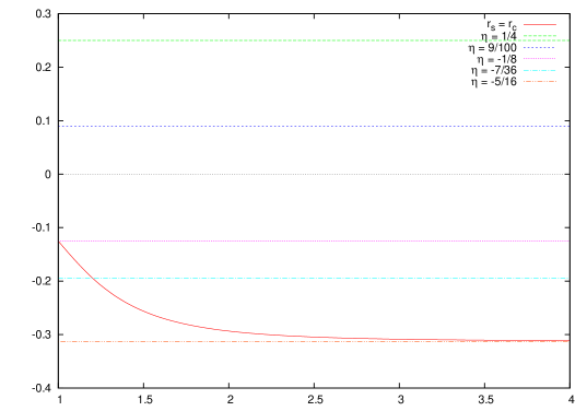
Figure 1: The bounds for $g(r_{s})\geq-1/2$ (83)(86) (red) on the $(r_{s}/r_{0},\eta)$-plane. Lines for $\eta=1/4,9/100,-1/8,-7/36,-5/16$ are also displayed.

In these cases, a solution to (81) satisfies $X>1$ for $r>r_{s}$ and it diverges at $r=r_{s}$ while there is no such solution for $r<r_{s}$. Moreover by studying the second order perturbations, it is indeed a local minimum of the functional (68). In this way, we find a smooth solution with the correct boundary condition and thus this gives the first candidate for $\gamma_{A}$ (as depicted in Fig.2(a)).

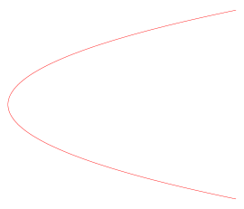
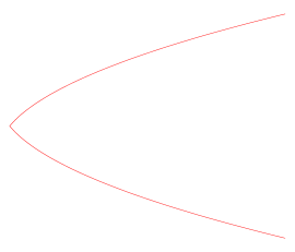
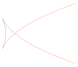
(a) smooth surface	(b) surface singular at $r=r_{*}$	(c) “switch-back” surface

Figure 2: Patterns of extremal curved surfaces $\gamma_{A}$ (projected on the $(r,x)$-plane). The integrand of (75) is locally minimum on the red lines and maximum on the blue one. Therefore we only have to consider (a) and (b).

Now we would like to turn to the other cases with $g(r_{s})<-1/2$. Since we cannot find smooth solutions, we need to be satisfied with a solution which is not smooth at the turning point $r=r_{*}$ as e.g. the one depicted in Fig.2(b), assuming that the minimal surface always exists. The existence of solution leads to another bound $r>r_{b}$, where $r_{b}$ satisfies

$$r_{s}^{6}f(r_{s})=\frac{4}{27}\frac{(g(r_{b})-1)^{3}}{g(r_{b})}\cdot r_{b}^{6}f(r_{b}).$$ (87)

For $r>r_{b}$, there are two solutions which satisfy $X>1$. The smaller is continuous through $r=r_{s}(>r_{b})$, and the greater is divergent in the limit $r\to r_{s}-0$. They get coincident at $r=r_{b}$ and disappear for $r<r_{b}$. Joining these, we can consider, for example, a “switch-back” surface like Fig.2(c). However, the second order perturbation of (75) is positive for the smaller solution, and negative for the greater. Then we need to consider only the first, and in this case the form of the surface is always like Fig.2(b).

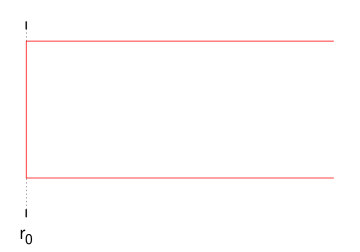
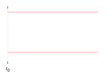
(d) connected at $r=r_{0}$	(e) disconnected

Figure 3: Two patterns of “trivial” $\gamma_{A}$. They have different values of $S_{A}$ due to the boundary term $q(r_{0})$, accounted only for (e). For $\eta<0$, (e) is preferred to (d), and vice versa for $\eta>0$.

Other than the solutions discussed above, there are two “trivial” candidates of the “minimal surface”. One is displayed in Fig.3(d), which is a pair of the surfaces $x=-l/2$ and $x=l/2$ connected at $r=r_{0}$. It is not a solution of the extremum equation $F(X)=0$ but on the edge of the configuration space of $x(r)$. The corresponding value of $S_{A}$ is, independently from $l$, given by substituting $r_{*}=r_{0}$ and $X\equiv 1$ to (75), resulting

$$S_{A}^{(d)} = \frac{\pi RV_{y}}{G_{N}^{(5)}\cdot L_{AdS}}\int_{r_{0}}^{r_{\infty}}(rg(r)+r)dr$$ (88)

$$= \frac{\pi RV_{y}}{2G_{N}^{(5)}\cdot L_{AdS}}\left[\left(1+2\eta f_{\infty}\right)r_{\infty}^{2}-r_{0}^{2}\right].$$

The other, which is displayed in Fig.3(e), is similar to it but different in an important way. Unlike the all variations of the surfaces discussed above, it consists of two parts which are not connected to each other. Therefore the corresponding value of $S_{A}$ includes the contribution from the boundary term $q(r_{0})=-{{4r_{0}^{2}}/{L^{2}L_{AdS}}}$ and

$$S_{A}^{(e)} = S_{A}^{(d)}-\frac{2\pi RV_{y}\cdot\eta L^{2}}{4G_{N}^{(5)}}q(r_{0})$$ (89)

$$= \frac{\pi RV_{y}}{2G_{N}^{(5)}\cdot L_{AdS}}\left[\left(1+2\eta f_{\infty}\right)r_{\infty}^{2}-\left(1-8\eta\right)r_{0}^{2}\right].$$

This is, as is expected, precisely twice of (66) except the difference of the divergent part coming from the boundary term. We can immediately see that, when $\eta<0$ the phase (e) is preferred to (d), and for $\eta>0$ (d) is preferred.

4.3 Numerical results and phase structures

Now we can numerically execute the integrals (75) and (79) for the solutions of the extremum equation (78), and plot the values on the $(l,S_{A})$-plane. We set the turning point $r_{*}$ as $r_{*}=r_{s}$ when $g(r_{s})\geq-\frac{1}{2}$, while we set it as $r_{*}=r_{b}$ when $g(r_{s})<-\frac{1}{2}$. These are because we find that they give the smallest values of the functional (68) when we change $r_{*}$ with $l$ fixed. The resulting behavior of $S_{A}(l)$ is plotted in Fig.4 ($\eta\geq 0$) and Fig.5 ($\eta\leq 0$). The zero point of $S_{A}$ is taken to be $S_{A}^{(d)}$ (88) for $\eta\geq 0$ and $S_{A}^{(e)}$ (89) for $\eta\leq 0$. The case for $\eta=0$ is the same one that was investigated in [24, 25].

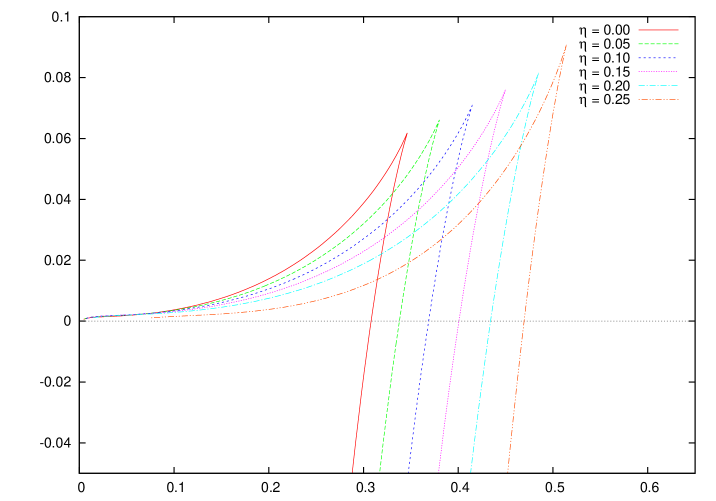
Figure 4: $(l,S_{A})$ plots for variable $0\leq\eta\leq{{1}/{4}}$. The unit for $l$ and $S_{A}$ are $R$ and ${{\pi V_{y}L}/{2G_{N}^{(5)}}}$, respectively. The value for the phase (d) is taken to be $0$ for $S_{A}$.

Where the curve $S_{A}=S_{A}(l)$ is below the $l$-axis, the corresponding nontrivially connected surface, given as the solution of the extremum equation, is the “minimal surface” $\gamma_{A}$ for each $l$. Otherwise the minimal surface is given by the “trivial” surfaces (d) or (e), depending on the sign of $\eta$. Therefore, when the line crosses the $l$-axis, there occurs a phase transition between those different phases as we mentioned before.

First look at Fig.4. We can see that the qualitative form of the curve does not change in the range $0\leq\eta\leq{{1}/{4}}$. The phase of the curved surface is preferred when $l$ is small, and there occurs a phase transition at some particular value $l=l_{c}$, for example, $l_{c}{/R}\simeq 0.338$ for $\eta=0.05$. Notice that nothing special happens around the causality upper bound $\eta=0.09$ (61).

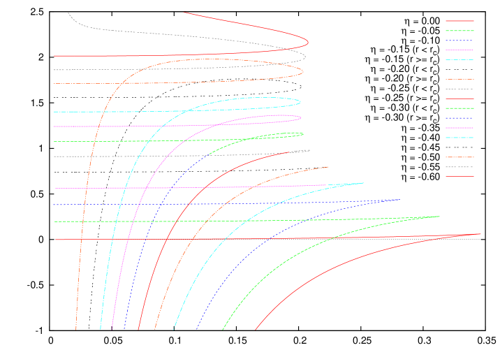
Figure 5: $(l,S_{A})$ plots for variable $\eta\leq 0$. The value for the disconnected phase (e) is taken to be $0$ for $S_{A}$.

The plots for $\eta<0$, displayed in Fig.5, may be more interesting. As we lower the value of $\eta$, the plotting curve changes its shape. Below $\eta=-1/8=-0.125$, the point corresponding to the boundary $r_{*}=r_{c}$ (86) between (a) and (b) walks on the curve from the origin toward the turning point. Just before it reaches there, when $\eta\simeq-0.209$, one (or more) loop(s) appears around there (Fig.6).

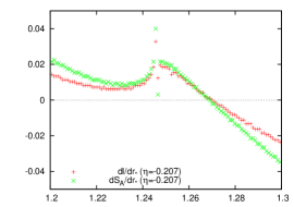
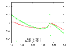
$\eta=-0.207$ ($r_{c}\simeq 1.2466$)	$\eta=-0.211$ ($r_{c}\simeq 1.2620$)	$\eta=-0.214$ ($r_{c}\simeq 1.2739$)

Figure 6: Plots for $dl/dr_{*}$ (red) and $dS_{A}/dr_{*}$ (green).

After that $r_{c}$ continues to walk downward until $\eta=-5/16=-0.3125$. Regardless the phenomena above, the phase structure is not altered. However, across $\eta=-0.548\dots$, the shape of the plotting curve changes dramatically, and below there, the curve is above the $l$-axis everywhere and so the disconnected phase is always favored (Fig. 7).

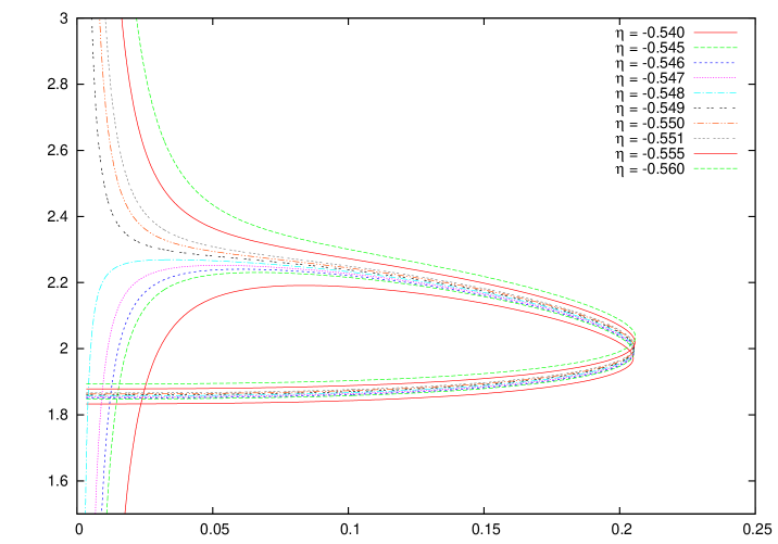
Figure 7: $(l,S_{A})$ plots for $\eta$’s around $-0.55$.

Note that these strange phenomena do not take places above the causality lower bound $\eta=-7/36=-0.1944\dots$ (61).

In summary, if we impose the causality bound (61), none of new phenomena found for the higher derivative theory such as the non-smooth surface as $\gamma_{A}$ like Fig.2(b), the loopy profile of $S_{A}(l)$, or the absence of phase transition, do not occur. In this sense, we can conclude that the higher derivative corrections does not largely change qualitative properties of HEE for AdS solitons. If we temporally forget the causality bound, then from the above analysis we can learn that there should be lower bound for $\eta$ otherwise the strange behaviors start to occur. For example, if we require that the non-smooth surfaces should not appear as $\gamma_{A}$, then we obtain the bound $\eta>-5/16$. Also, if we exclude the absence of phase transition, then we find $\eta>-0.548\cdot\cdot\cdot$. Moreover, if we consider the Gauss-Bonnet gravity literally without considering more higher derivative terms, then we will find that HEE is not well-defined for the region $\eta>0$ as we will explain in the next subsection.

4.4 Comments on an instability for $\eta>0$

Before we conclude this paper, we would like to point out an important fact for the conjectural formula (68) in the Gauss-Bonnet gravity. Consider a smooth surface $\gamma_{A}$ which minimizes the functional (68). We can assume that it is symmetric along $\theta$. Let us focus on the region near the turning point $r=r_{*}$, where we can treat the warp factor of the AdS space as a constant. In that region, we can simply ignore the $\theta$-direction and we can regard $\gamma_{A}$ as an effectively 2-dimensional surface in a flat 3-dimensional ambient space, spanned by $(r,x,y)$. In this setup, we can add infinitesimally small handles to $\gamma_{A}$ near $r=r_{*}$ and decrease the value of the $\int\!\sqrt{h}{\mathcal{R}}$ (i.e. the Euler number) without changing the other terms. Thus if we assume $\eta>0$, we can take (68) to be an arbitrarily small value and so there is no minimum of the this functional. In this way we find that HEE $S_{A}$ is ill-defined for $\eta<0$ in the Gauss-Bonnet gravity. This argument gets more clear in 4D Gauss-Bonnet gravity as the curvature contribution in (68) gets purely topological without focusing on near the turning points.

One may worry that our analysis for $\eta>0$ may be meaningless. However, this is not the case if we implicitly assume the presence of more higher derivative corrections in addition to the Gauss-Bonnet gravity, which will be the case in string theory. Indeed, we can show that the problem we mentioned occurs only when the higher order corrections are absent. In other words, what we find here is that if we consider the purely Gauss-Bonnet gravity in any dimension literally without any more higher derivative terms, then we will find that HEE is not well-defined when $\eta>0$.

5 Discussions and Summary

In this paper, we studied the holographic entanglement entropy (HEE) for AdS soliton geometries in the presence of higher derivative corrections. Our results in this paper show that the proposed higher derivative correction to HEE (68) behaves in a sensible way.

In the first half part, we calculated the leading higher derivative corrections due to ${\mathcal{R}}^{4}$ term for AdS soliton geometries in string theory and M-theory. Via the AdS/CFT, they are dual to the strong coupling expansions in the dual confining gauge theories such as a compactified ${\mathcal{N}}=4$ super Yang-Mills. Our result is qualitatively consistent with the free Yang-Mills calculation of the entanglement entropy.

In the latter half part, we studied the HEE for AdS solitons in the Gauss-Bonnet gravity. Especially we examined the dependence of HEE on the size of the subsystem $A$. If we restrict to the known causality bound of the Gauss-Bonnet parameter $\eta$, our result shows that the behavior of HEE and the structure of phase transition are qualitatively similar to that for Einstein gravity i.e. $\eta=0$. However, if we go beyond that bound, we observed several strange behavior such as the absence of phase transition and singular behavior of the solutions. We also find that if we consider the purely Gauss-Bonnet gravity literally without any more higher derivative terms, then we will find that HEE is not well-defined when $\eta>0$.

References

- [1]
- [2] J. M. Maldacena, “The large N limit of superconformal field theories and supergravity,” Adv. Theor. Math. Phys. 2 (1998) 231 [Int. J. Theor. Phys. 38 (1999) 1113] [arXiv:hep-th/9711200];
- [3] S. Ryu and T. Takayanagi, “Holographic derivation of entanglement entropy from AdS/CFT,” Phys. Rev. Lett. 96 (2006) 181602 [arXiv:hep-th/0603001]; “Aspects of holographic entanglement entropy,” JHEP 0608 (2006) 045 [arXiv:hep-th/0605073]; V. E. Hubeny, M. Rangamani and T. Takayanagi, “A Covariant holographic entanglement entropy proposal,” JHEP 0707 (2007) 062 [arXiv:0705.0016 [hep-th]].
- [4] M. Headrick and T. Takayanagi, “A Holographic proof of the strong subadditivity of entanglement entropy,” Phys. Rev. D 76 (2007) 106013 [arXiv:0704.3719 [hep-th]].
- [5] P. Hayden, M. Headrick and A. Maloney, “Holographic Mutual Information is Monogamous,” arXiv:1107.2940 [hep-th].
- [6] S. N. Solodukhin, “Entanglement entropy, conformal invariance and extrinsic geometry,” Phys. Lett. B 665, 305 (2008) [arXiv:0802.3117 [hep-th]].
- [7] R. Lohmayer, H. Neuberger, A. Schwimmer and S. Theisen, “Numerical determination of entanglement entropy for a sphere,” Phys. Lett. B 685, 222 (2010) [arXiv:0911.4283 [hep-lat]].
- [8] H. Casini and M. Huerta, “Entanglement entropy for the n-sphere,” Phys. Lett. B 694, 167 (2010) [arXiv:1007.1813 [hep-th]].
- [9] S. N. Solodukhin, “Entanglement entropy of round spheres,” Phys. Lett. B 693, 605 (2010) [arXiv:1008.4314 [hep-th]].
- [10] J. S. Dowker, “Hyperspherical entanglement entropy,” J. Phys. A 43 (2010) 445402 [arXiv:1007.3865 [hep-th]]; “Entanglement entropy for even spheres,” arXiv:1009.3854 [hep-th].
- [11] H. Casini, M. Huerta and R. C. Myers, “Towards a derivation of holographic entanglement entropy,” JHEP 1105 (2011) 036 [arXiv:1102.0440 [hep-th]].
- [12] M. Headrick, “Entanglement Renyi entropies in holographic theories,” Phys. Rev. D 82 (2010) 126010 [arXiv:1006.0047 [hep-th]].
- [13] P. Calabrese, J. Cardy and E. Tonni, “Entanglement entropy of two disjoint intervals in conformal field theory,” J. Stat. Mech. 0911 (2009) P11001 [arXiv:0905.2069 [hep-th]]; “Entanglement entropy of two disjoint intervals in conformal field theory II,” J. Stat. Mech. 1101 (2011) P01021 [arXiv:1011.5482 [hep-th]].
- [14] T. Nishioka, S. Ryu and T. Takayanagi, “Holographic Entanglement Entropy: An Overview,” J. Phys. A 42 (2009) 504008 [arXiv:0905.0932 [hep-th]].
- [15] P. Calabrese, J. Cardy, “Entanglement entropy and conformal field theory,” J. Phys. A42 (2009) 504005 [arXiv:0905.4013 [cond-mat]].
- [16] H. Casini and M. Huerta, “Entanglement entropy in free quantum field theory,” J. Phys. A 42 (2009) 504007 [arXiv:0905.2562 [hep-th]].
- [17] L. Y. Hung, R. C. Myers and M. Smolkin, “On Holographic Entanglement Entropy and Higher Curvature Gravity,” JHEP 1104 (2011) 025 [arXiv:1101.5813 [hep-th]].
- [18] J. de Boer, M. Kulaxizi and A. Parnachev, “Holographic Entanglement Entropy in Lovelock Gravities,” arXiv:1101.5781 [hep-th].
- [19] R. C. Myers and A. Sinha, “Seeing a c-theorem with holography,” Phys. Rev. D 82 (2010) 046006 [arXiv:1006.1263 [hep-th]]; R. C. Myers and A. Sinha, “Holographic c-theorems in arbitrary dimensions,” JHEP 1101 (2011) 125 [arXiv:1011.5819 [hep-th]].
- [20] D. V. Fursaev, “Proof of the holographic formula for entanglement entropy,” JHEP 0609 (2006) 018 [arXiv:hep-th/0606184].
- [21] M. T. Grisaru and D. Zanon, “SIGMA MODEL SUPERSTRING CORRECTIONS TO THE EINSTEIN-HILBERT ACTION,” Phys. Lett. B 177, 347 (1986); D. J. Gross and E. Witten, “Superstring Modifications of Einstein’s Equations,” Nucl. Phys. B 277, 1 (1986); M. D. Freeman, C. N. Pope, M. F. Sohnius and K. S. Stelle, “HIGHER ORDER sigma MODEL COUNTERTERMS AND THE EFFECTIVE ACTION FOR Phys. Lett. B 178, 199 (1986); Q. H. Park and D. Zanon, “MORE ON sigma MODEL BETA FUNCTIONS AND LOW-ENERGY EFFECTIVE ACTIONS,” Phys. Rev. D 35, 4038 (1987).
- [22] E. S. Fradkin and A. A. Tseytlin, “QUANTUM PROPERTIES OF HIGHER DIMENSIONAL AND DIMENSIONALLY REDUCED SUPERSYMMETRIC THEORIES,” Nucl. Phys. B 227, 252 (1983); M. B. Green and P. Vanhove, “D instantons, strings and M theory,” Phys. Lett. B 408, 122 (1997) [arXiv:hep-th/9704145]; M. B. Green, M. Gutperle and P. Vanhove, “One loop in eleven-dimensions,” Phys. Lett. B 409, 177 (1997) [arXiv:hep-th/9706175]; J. G. Russo and A. A. Tseytlin, “One loop four graviton amplitude in eleven-dimensional supergravity,” Nucl. Phys. B 508, 245 (1997) [arXiv:hep-th/9707134].
- [23] E. Witten, “Anti-de Sitter space, thermal phase transition, and confinement in gauge theories,” Adv. Theor. Math. Phys. 2 (1998) 505 [arXiv:hep-th/9803131].
- [24] T. Nishioka and T. Takayanagi, “AdS Bubbles, Entropy and Closed String Tachyons,” JHEP 0701 (2007) 090 [arXiv:hep-th/0611035].
- [25] I. R. Klebanov, D. Kutasov and A. Murugan, “Entanglement as a probe of confinement,” Nucl. Phys. B 796 (2008) 274 [arXiv:0709.2140 [hep-th]].
- [26] A. Pakman and A. Parnachev, “Topological Entanglement Entropy and Holography,” JHEP 0807 (2008) 097 [arXiv:0805.1891 [hep-th]].
- [27] A. Velytsky, “Entanglement entropy in d+1 SU(N) gauge theory,” Phys. Rev. D 77 (2008) 085021 [arXiv:0801.4111 [hep-th]].
- [28] P. V. Buividovich and M. I. Polikarpov, “Numerical study of entanglement entropy in SU(2) lattice gauge theory,” Nucl. Phys. B 802 (2008) 458 [arXiv:0802.4247 [hep-lat]]; “Entanglement entropy in gauge theories and the holographic principle for electric strings,” Phys. Lett. B 670 (2008) 141 [arXiv:0806.3376 [hep-th]].
- [29] Y. Nakagawa, A. Nakamura, S. Motoki and V. I. Zakharov, “Entanglement entropy of SU(3) Yang-Mills theory,” PoS LAT2009 (2009) 188 [arXiv:0911.2596 [hep-lat]]; “Quantum entanglement in SU(3) lattice Yang-Mills theory at zero and finite temperatures,” PoS LATTICE2010 (2010) 281 [arXiv:1104.1011 [hep-lat]].
- [30] P. Calabrese and J. L. Cardy, “Entanglement entropy and quantum field theory,” J. Stat. Mech. 0406, P06002 (2004) [arXiv:hep-th/0405152].
- [31] D. V. Fursaev and S. N. Solodukhin, “On the description of the Riemannian geometry in the presence of conical defects,” Phys. Rev. D 52, 2133 (1995) [arXiv:hep-th/9501127].
- [32] S. S. Gubser, I. R. Klebanov and A. W. Peet, “Entropy and temperature of black 3-branes,” Phys. Rev. D 54 (1996) 3915 [arXiv:hep-th/9602135].
- [33] J. Pawelczyk and S. Theisen, “AdS5 S5 black hole metric at O(),” JHEP 9809, 010 (1998) [arXiv:hep-th/9808126].
- [34] M. M. Caldarelli and D. Klemm, “M theory and stringy corrections to Anti-de Sitter black holes and conformal field theories,” Nucl. Phys. B 555 (1999) 157 [arXiv:hep-th/9903078].
- [35] R. Aros, M. Contreras, R. Olea, R. Troncoso, J. Zanelli, “Conserved charges for gravity with locally AdS asymptotics,” Phys. Rev. Lett. 84, 1647-1650 (2000) [gr-qc/9909015]; R. Olea, “Mass, angular momentum and thermodynamics in four-dimensional Kerr-AdS black holes,” JHEP 0506, 023 (2005) [hep-th/0504233]; O. Miskovic, R. Olea, Phys. Rev. D79, 124020 (2009) [arXiv:0902.2082 [hep-th]].
- [36] A. Buchel and R. C. Myers, “Causality of Holographic Hydrodynamics,” JHEP 0908 (2009) 016 [arXiv:0906.2922 [hep-th]].
- [37] R. C. Myers and J. Z. Simon, “Black Hole Thermodynamics in Lovelock Gravity,” Phys. Rev. D 38 (1988) 2434.
- [38] D. G. Boulware, S. Deser, “String Generated Gravity Models,” Phys. Rev. Lett. 55, 2656 (1985).
- [39] R. G. Cai, “Gauss-Bonnet black holes in AdS spaces,” Phys. Rev. D 65, 084014 (2002) [arXiv:hep-th/0109133].
- [40] R. G. Cai, S. P. Kim and B. Wang, “Ricci flat black holes and Hawking-Page phase transition in Gauss-Bonnet gravity and dilaton gravity,” Phys. Rev. D 76, 024011 (2007) [arXiv:0705.2469 [hep-th]].