Complex Structure in Class 0 Protostellar Envelopes II: Kinematic Structure from Single-Dish and Interferometric Molecular Line Mapping

Abstract

We present a study of dense molecular gas kinematics in seventeen nearby protostellar systems using single-dish and interferometric molecular line observations. The non-axisymmetric envelopes around a sample of Class 0/I protostars were mapped in the N₂H⁺ ($J=1\rightarrow 0$) tracer with the IRAM 30m, CARMA and PdBI as well as NH₃ (1,1) with the VLA. The molecular line emission is used to construct line-center velocity and linewidth maps for all sources to examine the kinematic structure in the envelopes on spatial scales from 0.1 pc to $\sim$1000 AU. The direction of the large-scale velocity gradients from single-dish mapping is within 45^∘ of normal to the outflow axis in more than half the sample. Furthermore, the velocity gradients are often quite substantial, the average being $\sim$2.3 km s^-1 pc^-1 . The interferometric data often reveal small-scale velocity structure, departing from the more gradual large-scale velocity gradients. In some cases, this likely indicates accelerating infall and/or rotational spin-up in the inner envelope; the median velocity gradient from the interferometric data is $\sim$10.7 km s^-1 pc^-1 . In two systems, we detect high-velocity HCO⁺ ($J=1\rightarrow 0$) emission inside the highest-velocity N₂H⁺ emission. This enables us to study the infall and rotation close to the disk and estimate the central object masses. The velocity fields observed on large and small-scales are more complex than would be expected from rotation alone, suggesting that complex envelope structure enables other dynamical processes (i.e. infall) to affect the velocity field.

1 Introduction

Infall and rotation in dense cores and protostellar envelopes both play important roles in the formation of protostars and their surrounding disks. Infall must be taking place in the envelopes because we observe newborn protostars embedded within their natal clouds. The two classic analytic theories of collapse describe infall as either being outside-in (Larson, 1969) or inside-out (Shu, 1977). The initial angular momentum of the protostellar cloud governs the formation and sizes of the proto-planetary disks (e.g. Cassen & Moosman, 1981; Terebey et al., 1984) and will affect the ability of the cloud core to fragment into multiple stellar systems (e.g. Burkert & Bodenheimer, 1993; Bonnell & Bate, 1994). The ubiquitous formation of proto-planetary disks (Haisch et al., 2001; Hernández et al., 2007) and the prevalence of binary systems (Raghavan et al., 2010) lends strong indirect evidence for the presence of rotation. Therefore, observing these two processes in protostellar envelopes has enormous potential for constraining star formation theory through comparisons to analytic models and numerical simulations. Dense protostellar cores are well known as sites of isolated, low-mass star formation (e.g. Shu et al., 1987; Benson & Myers, 1989; McKee & Ostriker, 2007) and are the ideal place to study the kinematic structure from large, core/envelope scales ($\sim$0.1 pc) down to scales near the disk radius.

Several previous studies have attempted to characterize the rotation in dark clouds and dense cores. Arquilla & Goldsmith (1986) examined the kinematic structure of dark clouds using CO on $\sim$10′ scales, finding that some exhibit possible rotation signatures derived from velocity gradients. Later, Goodman et al. (1993) and Caselli et al. (2002) used the dense molecular tracers NH₃ and N₂H⁺ to examine rotation in the dense cores within dark clouds ($\sim$2-3′ scales). Goodman et al. (1993) and Caselli et al. (2002) found typical velocity gradients of $\sim$1 to 2 km s^-1 pc^-1 , which were interpreted to be slow, solid-body core rotation. However, the observations had limited resolution (60″-90″), nearly the size of the envelopes in some cases. Rotation is not necessarily solid-body; however, this assumption simplifies analysis in terms of equipartition and the early data did not warrant more sophisticated models.

Caselli et al. (2002) noted that their finer resolution as compared to Benson & Myers (1989) revealed clear deviations from linearity in the velocity gradients. This indicates that the velocity structure of cores may be more complex than simply axisymmetric, solid-body rotation. Chen et al. (2007) carried out a higher resolution study using interferometric observations of N₂H⁺ from OVRO on a sample of protostars in the Class 0 (André et al., 1993) and Class I phases (Lada, 1987). They found substantially larger velocity gradients in the inner envelopes, with complex velocity fields, only showing probable rotation signatures in a few cases.

While the possible rotation has been probed using optically thin tracers, the study of infall in protostellar envelopes has been limited to observations of optically thick tracers toward the envelope center. Zhou et al. (1993) and Myers et al. (1995) used observations of CS and H₂CO to infer the detection of infall in the envelope of the Class 0 protostar B335. The optically thick molecular lines are self absorbed at the line-center and the key signature of infall is the blue-shifted side of the line being brighter than the red-shifted side. Later, Di Francesco et al. (2001) found inverse-P Cygni line profiles in H₂CO which are interpreted as infall. Furthermore, infall at large-scales may have been detected in the pre-stellar core L1544 (Tafalla et al., 1998).

These previous studies have interpreted the kinematic structure in terms of axisymmetric envelopes. However, our recent studies (i.e. Tobin et al., 2010b; Looney et al., 2007) have revealed that the dense envelopes surrounding the youngest, generally Class 0, protostars often have complex, non-axisymmetric morphological structure (also see Benson & Myers, 1989; Myers et al., 1991; Stutz et al., 2009). Out of the 22 protostellar systems exhibiting extinction at 8$\mu$m, only three appeared to be roughly axisymmetric. We suggested that the asymmetric envelope structure may play a role in the formation of binary systems by making fragmentation easier and that the initial disk structure may be perturbed from uneven mass loading. However, in order to understand the effects that complex envelope structure has on disk formation and fragmentation, the kinematics of the dense gas must be characterized.

Given the apparent prevalence of complex morphological structure in protostellar envelopes, the kinematics of the envelopes must also be studied on scales such that the morphological structure is spatially resolved. To examine the kinematic structure of morphologically complex envelopes, we have undertaken a molecular line survey focusing on nearby (d $<$ 500 pc), embedded protostars drawn from our sample of envelopes in Tobin et al. (2010b). We have approached this study from two directions. First, we obtained new single-dish N₂H⁺ mapping of sixteen systems with the IRAM 30m, a factor of two improvement in resolution over Caselli et al. (2002). Secondly, we obtained new interferometric N₂H⁺ and NH₃ observations of fourteen systems with resolutions between 3.5″ and 6″. The analysis of both the single-dish and interferometric observations offers a comprehensive view of the kinematic and morphological structure from 0.1 pc scales down to $\sim$1000 AU. Complementary Spitzer imaging gives us a clear view of the outflow angular extent and direction in all of these objects.

In this paper, we are primarily presenting the dataset as a whole and give a basic analysis of each object; an upcoming paper will give a more detailed interpretation of the velocity structures. The data for each object are quite rich and we find many envelopes with velocity gradients normal to the outflow on large-scales in the single-dish maps, persisting down to small-scales in the interferometer maps. We have organized the paper as follows: Section 2 discusses the sample, observations, data reduction, and analysis, Section 3 presents our general results and discusses each object in detail, and Section 4 discusses the basic overall properties of the sample as a whole.

2 Observations and Data Reduction

We mapped the protostellar envelopes in the dense gas tracers NH₃ and N₂H⁺, which are known to be present over a wide range of spatial scales and preferentially trace high density regions (critical densities of $\sim$2$\times$10³ cm^-3 (Danby et al., 1988; Schöier et al., 2005) and $\sim$1.4$\times$10⁵ cm^-3 (Schöier et al., 2005) respectively), where CO has depleted (e.g. Bergin et al., 2002; Tafalla et al., 2004). The single-dish data were all obtained using the IRAM 30m telescope, mapping N₂H⁺ ($J=1\rightarrow 0$). The single-dish observations were followed by interferometric observations of N₂H⁺ ($J=1\rightarrow 0$) using CARMA and the Plateau de Bure Interferometer, in addition to NH₃ (1,1) observations using the VLA, including VLA archival data for some objects. We will briefly describe the observations and the data analysis procedure for each data set.

2.1 The Sample

Our sample of protostellar envelopes selected for kinematic study is directly drawn from the objects presented in Tobin et al. (2010b, hereafter Paper I). All protostellar systems observed have a surrounding envelope visible in 8$\mu$m extinction. Much of the envelope sample was found within archival Spitzer data from the cores2disks (c2d) legacy program (Evans et al., 2009). Given that c2d and most other archival observations were short integrations, we were only able to detect very dense structures which happened to have a bright backgrounds at 8$\mu$m. Thus, there may be a bias towards denser envelopes, but the range of bolometric luminosity is fairly broad with objects $<$1 $L_{\sun}$ and as much as $\sim$14 $L_{\sun}$. These protostars are listed in Table 1 and are mostly Class 0 systems with a few Class Is. The requirement of having an envelope visible in extinction enables us to consider the envelope morphology in our interpretation of the kinematic data. We regard the 8$\mu$m extinction to more robustly reflect the structure of high density material around the protostars on scales $>$ 1000 AU, as molecular tracers may have abundance variations which affect their spatial distribution. The requirement of 8$\mu$m extinction also biases the sample to more isolated systems, only Serpens MMS3 and L673 have multiple neighbors $<$ 0.1 pc away.

2.2 IRAM 30m Observations

We observed our sample of protostellar envelopes in two observing runs at the IRAM 30m radio telescope on Pico Veleta in the Spanish Sierra Nevada. The first observing run took place between 2008 December 26 - 30; during this run we only observed four protostars due to poor weather. We used the AB receiver system and observed the protostars in the N₂H⁺ ($J=1\rightarrow 0$) transition ($\nu_{\rm rest}$= 93.1737637 GHz; $JF_{1}F=123\rightarrow 012$ component (Keto & Rybicki, 2010)); the half power beam width (HPBW) of the 30m at this frequency is $\sim$27″. The second observing run took place between 2009 October 22-26 using the new Eight MIxer Receiver (EMIR). We observed thirteen protostars and revisited L1527 from the first run, using the VESPA auto-correlation spectrometer as the backend for all observations. Single-sideband system temperatures of 130 K at $\nu$= 93 GHz were typical for both observing runs. During the 2008 run we used the 20 MHz bandwidth mode with 20kHz channels and in 2009 we used 40 MHz with 20kHz channels; see Table 2 the list of sources observed and more detail.

We conducted our observations using frequency-switched on-the-fly (OTF) mapping mode. The maps varied in size depending on the extent of the source being observed, most being 3^′ $\times$ 3^′. Most maps were integrated down to at least $\sigma_{T}$ $\sim$ 150mK for the N₂H⁺ ($J=1\rightarrow 0$) transition, noise levels for each map are listed in Table 2. We mapped the sources by scanning in the north-south direction and again in the east-west direction to minimize striping in the final map. The scan legs were stepped by 5″ and we repeated the maps to gain a higher signal-to-noise ratio. Calibration scans were taken about every 10 minutes between scan legs and the final maps took approximately 2 hours to complete. Pointing was checked about every two hours, azimuth and elevation offsets were typically $\pm$5″; the pointing offset remained stable, typically within $\sim$2″ during an observation. These values agree well with the rms pointing accuracy of $\sim$2″.

The initial calibration of the OTF data to the antenna temperature scale and CLASS data format was performed automatically on-site by the Multichannel Imaging and calibration software for Receiver Arrays (MIRA) package. Further data reduction was done using CLASS (part of GILDAS). For all molecular lines observed, the frequency switched spectra were folded and baseline subtracted using a second order polynomial. We then reconstructed the spectral map on a grid such that the FWHM of the beam was spanned by 3 pixels and each pixel is the average of all measurements within the FWHM of the beam.

2.3 CARMA Observations

The CARMA observations were taken in four observing semesters; most sources were observed solely in the D-array configuration (except L1527 and L1157 see below) which yields $\sim$6″ resolution. Three objects were observed in 2009 July and August. The correlator at this time only had three bands, operating dual side-band mode, giving 6 spectral windows and was configured for an IF frequency of 91.181 GHz. N₂H⁺ ($J=1\rightarrow 0$) and HCO⁺ ($J=1\rightarrow 0$) ($\nu_{\rm rest}$=89.188518 GHz; (Lovas, 1992)) were observed in opposite side-bands of one spectral window with 2MHz bandwidth and 63 channels giving $\sim$0.1 km/s velocity resolution. The N₂H⁺ ($J=1\rightarrow 0$) emission spectrum comprises 7 hyperfine lines over $\sim$ 17 km s^-1, consisting of two groups of three lines and a single isolated line. The 2MHz window is too narrow to observe all the lines; therefore, we observed the strongest set of three lines, rather than observing the isolated line to maximize our signal-to-noise. The multiple hyperfine transitions enables the optical depth and excitation temperature to be determined. The second band was also configured for 2 MHz bandwidth and was centered on the main hyperfine component of the HCN ($J=1\rightarrow 0$) transition ($\nu_{\rm rest}$=88.6318473 GHz; (Lovas, 1992)), and the third band was configured for continuum observations with 500 MHz bandwidth (1 GHz dual-side band).

Another set of sources was observed in 2010 April and May. During this time, a new correlator was being completed with higher velocity resolution over a wider bandwidth and more spectral windows; most data were taken with six bands (twelve spectral windows). For these observations, the IF frequency was set to 90.9027 GHz such that N₂H⁺ ($J=1\rightarrow 0$) and HCN ($J=1\rightarrow 0$) could be observed in opposite side-bands of the same correlator band. We also observed HCO⁺ ($J=1\rightarrow 0$), H¹³CO⁺ ($J=1\rightarrow 0$) ($\nu_{\rm rest}$= 86.754294 GHz), ortho-NH₂D ($1_{1,1}\rightarrow 1_{0,1}$), ($\nu_{\rm rest}$= 85.926263 GHz), and continuum; rest frequencies for these transitions are taken from Lovas (1992). All spectral line observations used 8 MHz bandwidth with 385 channels yielding $\sim$ 0.06 km s^-1 velocity resolution, during reduction this was rebinned to 0.1 km s^-1 resolution to reduce noise. The continuum observations again had 500 MHz bandwidth (1 GHz dual-side band). See Table 3 for exact dates of observation for particular sources.

In addition, L1527 and L1157 were observed in E-array configuration in 2008 October and L1157 was again observed in D-array in 2009 March. These observations were taken in a three-point mosaic pattern to better recover the large-scale emission from the envelopes. The correlator was configured with one band for continuum, the other two bands were set to observe N₂H⁺ ($J=1\rightarrow 0$) and HCO⁺ ($J=1\rightarrow 0$). One band had 2MHz bandwidth and was centered on the isolated N₂H⁺ component. The other band was configured with 8 MHz bandwidth and 63 channels with 0.4 km s^-1 resolution to cover all 7 N₂H⁺ ($J=1\rightarrow 0$) hyperfine lines. However, we only use the 0.1 km s^-1 velocity resolution data for kinematics. The observations of L1157 are further detailed in Chiang et al. (2010).

All datasets were observed in a standard loop (calibrator–source–calibrator), a bright quasar within 15^∘ was used for phase and amplitude calibration. The calibrator was integrated for 3 minutes while the source was integrated for 15 minutes in each cycle. Absolute flux calibration was obtained by observing standard flux calibration sources, see Table 3. Bandpass calibration for the continuum bands was accomplished by observing a bright quasar, generally 3C454.3; the spectral line bands were bandpass corrected using the noise source.

Each dataset was processed using the MIRIAD software package (Sault et al., 1995). The raw visibilities were corrected for refined antenna baseline solutions and transmission line-length variation. The data were then edited to remove uncalibratable data (i.e. poor phase coherence, phase jumps, anomalous system temperatures/amplitudes). The bandpass corrections were computed using the mfcal routine. The absolute flux calibration was derived using the bootflux routine which determines the flux density of the gain calibrator relative to the flux calibration source (absolute calibration uncertainty is typically $\sim$10%). The phases and amplitudes were calibrated using the mselfcal routine. The phase and amplitude solution calculated for the continuum bands was then transferred to the spectral line bands. Continuum images and spectral line cubes were generated by inverting the corrected visibilities with natural weighting, creating the dirty map. Then the dirty map is CLEANed using the mossdi routine using a clean box of 60^′′ x 60^′′ which fits within the primary beam of the 10.4m dishes ($\sim$72″ at $\lambda$=3.2mm). In this paper, we will mainly interpret the N₂H⁺ data but will comment on the other molecules when relevant and the 3mm continuum data are presented in the Appendix.

2.4 VLA Observations

The NH₃ (1,1) observations were taken with EVLA transition system during the final semester of VLA correlator operation in D configuration. Eight-hour tracks were taken for 5 sources during 2009 October, November, and 2010 January (see Table 4). We used the 4 IF mode providing two tunings and dual-polarization to observe the NH₃ (1,1) and (2,2) inversion transitions ($\nu$=23.6944955, 23.7226336 GHz respectively (Ho & Townes, 1983)) with 1.5 MHz bandwidth and 127 channels yielding $\sim$0.15 km/s velocity resolution. This configuration was able to observe the main component and two sets of satellite lines for the NH₃ (1,1) transition. We alternately observed the source and a calibrator within 15^∘. Two minutes were spent integrating on the calibrator while ten minutes were spent on the target during each cycle. Pointing was updated every hour, 3C84 was observed as the bandpass calibrator and 3C48 or 3C286 was used for absolute flux calibration.

The raw visibility data from the VLA were reduced and calibrated using the CASA (Common Astronomy Software Applications) package. The task importvla was used to convert the VLA data to a CASA measurement set. The visibility data were then inspected and edited, specifically flagging shadowed data and any VLA antennas. Only EVLA antennas were used in our final dataset because we used doppler tracking during the observations, which caused phase jumps between VLA and EVLA antennas. Antenna positions were corrected using the gencal task when necessary and the absolute flux scale was set using the setjy task (absolute calibration uncertainty is typically 10%). The phases and amplitudes were calibrated using the gaincal task; the bandpass correction was determined using the bandpass task. All the calibrations were then applied using the applycal task. We then inspected the corrected data to ensure proper phase correction; any severely outlying amplitude points in the source data were also flagged.

The final spectral datacubes were generated using the clean task. The clean task encompasses several individual processes including inverting the visibilities, CLEANing the image, and restoring the image. Since the VLA provides a 2^′ diameter primary beam (field of view), we took several additional steps to increase our final image fidelity. We first performed a first-pass CLEANing of a spectral data cube over the 2^′ primary beam. Then we calculated the integrated intensity of the main component of the NH₃ (1,1) or (2,2) transition by summing the spectral line channels. Next, we created a mask image in which pixels below a 2$\sigma$ intensity threshold were rejected and those above were kept. This isolated the area of NH₃ emission around a particular protostar enabling CLEANing down to near a 1$\sigma$ threshold. Then for the NH₃ (1,1) images, we employed the multi-scale CLEAN algorithm (Rich et al., 2008); this algorithm models they sky as the sum of Gaussian components of various widths, which for extended sources works better than modeling the sky as the sum of many point source CLEAN components. In this paper, we will only present the NH₃ (1,1) data.

In addition to our own observations, we include VLA archival data for the sources L1527, L1521F, and L483. The data for L1521F and L483 were taken in different correlator configurations than our observations, see Table 4. The same reduction procedure was applied for these archival data as for our observations.

2.5 Plateau de Bure Interferometer Observations

L1157 was observed with the Plateau de Bure Interferometer on 2009 June 17 and 2009 July 8 in the D-array configuration with 5 antennas operating. It was observed again on 2009 November 13 in C-array configuration with 6 antennas. During the first track the weather conditions were average, with 5 to 10 mm of precipitable water vapor (pwv), respectively and a RMS phase noise lower than 64°. During the last two tracks the weather conditions were better, with 3-6 mm and 5-7 mm of pwv and a RMS noise phase lower than 41° and 24°, respectively

The 3mm receivers were tuned to the N₂H⁺ ($J=1\rightarrow 0$) transition in the lower-sideband. The correlator was configured with two windows for continuum observation, each having 320 MHz of bandwidth and one window with 20 MHz bandwidth for the N₂H⁺ ($J=1\rightarrow 0$), yielding a velocity resolution of 0.125 km/s. Both the spectral line and continuum observations were taken in dual-polarization mode.

The raw data were calibrated using the CLIC program from the GILDAS software package. A standard calibration procedure was used. Visibilities amplitudes and phases for each baseline were inspected and bad data (e.g. affected by phase jumps or antenna shadowing) were flagged. Phases were then calibrated using observations of the 1927+739 calibrator. Absolute flux was derived from observations of MWC349, assuming a flux of 1.15 Jy at 3 mm for that source; uncertainty in the absolute flux is $\sim$10%.

The calibrated data were then reduced using the MAPPING program from GILDAS. A UV table was created for the 3mm continuum as well as for the N₂H⁺ ($J=1\rightarrow 0$) line. The 3mm continuum visibilities were then subtracted from the line visibilities. Finally, a deconvolved map was produced using the the CLEAN algorithm. The synthesized beam in the final map is roughly circular with a FWHM of $\sim 3.4\times 3.3\arcsec$ at PA 114^∘; further details of the observations are listed in Table 5.

2.6 Data Analysis

2.6.1 Hyperfine Fitting

The N₂H⁺ and NH₃ molecular lines both have a hyperfine emission line spectrum. This allows us to robustly determine the line-center velocity and full-width half-maximum (FWHM) linewidths in each pixel by fitting all the hyperfine components simultaneously. We can fit the line-center velocities substantially better than native resolution of the observations. Goodman et al. (1993) approximates the observed velocity accuracy as

$$\sigma_{v}=1.15\left(\frac{\sigma_{T}}{T_{peak}}\right)(1.21\delta_{v}\Delta v)^{1/2}.$$ (1)

This assumes that the lines have a Gaussian shape, $\sigma_{T}$ is the rms noise, $T_{peak}$ is the peak line intensity, $\Delta v$ is the FWHM linewidth, and $\delta_{v}$ is the velocity width of the channels. The additional factor 1.21 is the intrinsic error in the autocorrelation spectrometer with unity weighting (Thompson et al., 2001). Using this relationship for velocity accuracy, if we had a signal-to-noise of 5, assuming $\Delta v$ = 0.3 km s^-1and $\delta_{v}$=0.1 km s^-1, our velocity accuracy would be 0.043 km s^-1. Note that this is the velocity accuracy for one line, using the multiple hyperfine components of N₂H⁺ and NH₃ we can obtain even greater accuracy.

To fit the lines, we applied the CLASS hyperfine fitting routines to each line. The hyperfine frequencies and line ratios for N₂H⁺ ($J=1\rightarrow 0$) were taken from Keto & Rybicki (2010) and we use the NH₃ frequencies and line ratios that are built into CLASS (Rydbeck et al., 1977; Ho & Townes, 1983). A semi-automated routine was used for fitting the hyperfine structure across the entire spectral map. We first generated an integrated intensity map of the central three hyperfine lines, from this map we selected each pixel with 3$\sigma$ detection of N₂H⁺ or NH₃ and then generated a CLASS script to fit the hyperfine structure at each point and write out a table containing these data. The fitting does not require all hyperfine components to have 3$\sigma$ detections, only that there are clear detections of the strongest hyperfine lines. Points where the fitting failed due to inadequate signal-to-noise were removed from the final table. The table is then used for plotting maps of the velocity field, linewidth, optical depth, and excitation temperature, all of which are all determined from fitting the hyperfine structure. The zeroth-moment maps (integrated intensity) are computed simplistically by measuring the intensity of the hyperfine lines within a given velocity range, summing the emission, and multiplying by the channel velocity width. The basic emission properties of N₂H⁺and NH₃ are separated into three tables: Table 6 for the single-dish N₂H⁺, Table 7 for the interferometric N₂H⁺, and Table 8 for the VLA NH₃ data. These tables list the line center velocities, linewidths, maximum integrated intensities, total optical depth of the transition (sum of optical depths for each component), excitation temperature, column density (following Goldsmith & Langer (1999) for N₂H⁺ and (Bourke et al., 1995) for NH₃), envelope mass as a function of assumed abundance, and approximate envelope radii.

2.6.2 Velocity Gradient Fitting

Using the line center velocities computed from the hyperfine fitting, the velocity gradients are computed for each object in three ways. First we simply computed the velocity difference between two points offset from the protostar by 10000 AU, normal to the outflow direction, and divided by the distance. Second, we computed a linear fits to cuts through the velocity data, taken normal to the outflow using points within $\pm$30″ of the protostar and/or within the region of the cloud directly associated with the protostar. Lastly, we fit a plane to the entire velocity field using the method described in Goodman et al. (1993), but using our own IDL implementation coupled with the MPFIT routines (Markwardt, 2009). We fit the line-center velocity field with the function

$$v_{LSR}=v_{0}+a\Delta\alpha+b\Delta\delta$$ (2)

where $v_{0}$ is the systemic velocity, $\Delta\alpha$ and $\Delta\delta$ are offsets in right ascension and declination (in arcseconds) and $a$ and $b$ are the velocity gradients per arcseconds in the $\alpha$ and $\delta$ directions respectively. The total velocity gradient is then given by

$$g=(a^{2}+b^{2})^{1/2}\times\frac{206264.98}{D}$$ (3)

with a position angle (PA) east of north (toward increasing velocity) given by

$$\theta_{g}=tan^{-1}\frac{b}{a}$$ (4)

where D is the distance in parsecs and the constant is the number of arcseconds per radian. We use all three methods on the single-dish data and only the latter two methods on the interferometer data since the extent of N₂H⁺ and NH₃ emission varies widely from object to object.

2.7 Extended Structure Sensitivity

As a general rule, interferometers filter-out large-scale emission; however, if there is a velocity gradient and the lines are well-resolved, the largest scale of emission in a given channel may only be a fraction of the full structure. Thus, different portions of the envelopes become visible in different velocity channels and the integrated intensity maps (zeroth-moment) build a picture of the envelope emission from the multiple velocity components. If all of this emission had resided in one velocity channel, substantially more emission would have been filtered-out. Furthermore, the filamentary nature of many envelopes enabled them to be viewed over a larger area than an envelope that fills the primary beam more evenly.

We do not combine the single-dish and interferometer data because each probe different size scales and it is often advantageous to have the large-scale emission resolved-out of the interferometer maps. Resolving-out the large-scale emission isolates the regions of compact emission in the inner envelope where there may be significant detail in the velocity field. Furthermore, our analysis of only the kinematic structure does not necessitate recovery of all flux; a detailed summary of the steps needed to combine single-dish data with CARMA observations is given in Koda et al. (2011).

3 Results

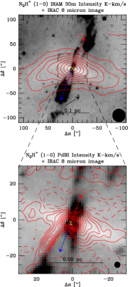
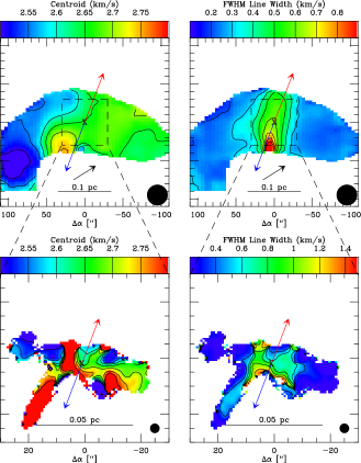
Figure 1: L1157– The top row shows the data from the IRAM 30m and the bottom row shows the PdBI data. In the left column, the 8$\mu$m IRAC images with N₂H⁺ ($J=1\rightarrow 0$) integrated intensity contours overlaid. The IRAM 30m contours start at the 10$\sigma$ level and increase in 20$\sigma$ increments while the PdBI data start at the $\pm$5$\sigma$ level and increase in 20$\sigma$ increments, see Tables 6 - 8 for values of $\sigma_{I}$. The middle column shows the line-center velocity fit of the N₂H⁺ emission across the envelope and the right column shows the FWHM linewidth. The red and blue lines mark the central axis of the outflow and their respective orientation in the plane of the sky; the X marks the position of the protostar from dust continuum and/or 24$\mu$m emission and the black arrows indicate the direction of the velocity gradient derived from the velocity field. The velocity gradient direction for the PdBI data could not be fit for L1157. The single-dish data show an ordered velocity gradient along the filamentary envelope, following the high density region as it curves south. The interferometer map also reflects this velocity gradient, but there is a reversal with red-shifted emission just east of the protostar. There is also a red-shifted feature that appears in the interferometer and single-dish map just southeast of the protostar, this appears to be due to outflow interaction given its location along the cavity wall. Both the single-dish and interferometer maps have large linewidths near the protostar, which appears to be due to outflow interaction. Reference positions for the observations are listed in Tables 2 and 5.

We mapped the regions around each protostar where we detected the presence of 8$\mu$m extinction in Paper I. Each envelope was observed to be a bright source of N₂H⁺ ($J=1\rightarrow 0$) (hereafter N₂H⁺) emission in the single-dish data; N₂H⁺ emission was present over much of the area where we detect extinction at 8$\mu$m in each map, shown in Figures 1 through 23. N₂H⁺ and NH₃ (1,1) (hereafter NH₃) is also detected toward all sources in the interferometer data. The interferometer observations select out the regions of brightest, compact emission which are usually associated with the densest regions of the protostellar envelope. Furthermore, there are many cases where the N₂H⁺ or NH₃ emission peak is not centered on the protostar in the single-dish and/or interferometer observations (see Section 4.5). The protostar positions in Figures 1 through 23 are derived from their 3mm continuum source, which is often coincident with the 8$\mu$m point source (see Appendix), or the 24$\mu$m source where continuum data were not available.

We know the outflow direction and the angular width of the cavity for all objects in the sample from the Spitzer IRAC data. This gives an observational constraint on the region in which the outflow may impact the envelope. These data enable the characterization of kinematic properties of the envelopes and determination of the origin of the kinematic structure. We can determine whether the kinematics reflect the intrinsic velocity structure of the core/envelope or if the outflow is likely affecting the observed kinematics. Such distinction is critical to ensure that we are not misled in further interpretation. While kinematic information is missing from the Spitzer images (i.e. blue and red-shifted sides traced by CO emission), this information is readily available in the literature for most objects (Table 1). Note that we can also often infer the blue and red-shifted outflow directions from the scattered light morphology and intensity (Whitney et al., 2003).

3.1 Similarity of N₂H⁺ and NH₃ Emission Properties

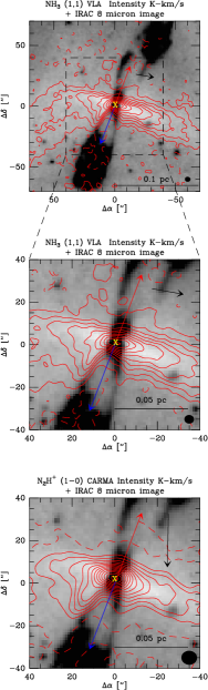
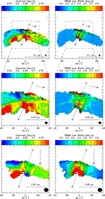
Figure 2: L1157– The top and middle rows show the VLA NH₃ (1,1) data while the bottom row shows the CARMA N₂H⁺ ($J=1\rightarrow 0$) data. In the left column, the 8$\mu$m IRAC images with integrated intensity contours overlaid. The VLA contours start at the $\pm$3$\sigma$ level and increase in 6$\sigma$ increments while the CARMA data start at the $\pm$3$\sigma$ level and increase in 3$\sigma$ increments, see Tables 6 - 8 for values of $\sigma_{I}$. The middle column shows the line-center velocity of the gas across the envelope and the right column shows the FWHM linewidth. The red and blue lines mark the central axis of the outflow and their respective orientation in the plane of the sky; the X marks the position of the protostar from dust continuum and 24$\mu$m emission and the black arrows indicate the direction of the velocity gradient derived from the velocity field. Notice the close correspondence of the intensity distribution and line kinematics between the NH₃ and N₂H⁺ maps indicating that they are likely tracing the same material. Reference positions for the observations are listed in Tables 2 - 5.

Since our interferometric observations mapped either NH₃ or N₂H⁺ for most protostars and our single-dish data solely mapped N₂H⁺, it is important to demonstrate that the kinematic structure observed in the two tracers is consistent. We have observed the envelope around L1157 in N₂H⁺ with the IRAM 30m, CARMA (Chiang et al., 2010), and the PdBI, while observing it in NH₃ with the VLA. The NH₃ and N₂H⁺ emission both closely follow the regions of 8$\mu$m extinction as shown in Figures 1 and 2 and the velocity maps have a very similar structure. The similar spatial emission and kinematic properties indicate that emission from these molecular species arises from approximately the same region of the envelope (from 0.1 pc to 1000 AU). Further comparisons of our sample can be made to data in the literature: Chen et al. (2007) for CB230 and IRAS 03282+3035, L1527 with Goodman et al. (1993), HH211 with Tanner & Arce (2011), and L483 with Fuller & Wootten (2000). In all these cases, the N₂H⁺ and NH₃ emission is detected in the same regions of the envelope with similar kinematic properties. This confirms that N₂H⁺ and NH₃ trace similar physical conditions at the level of precision we are probing, in agreement with the results from Johnstone et al. (2010). Section 4.5 further discusses the impact of chemistry on these species.

3.2 Velocity Gradients

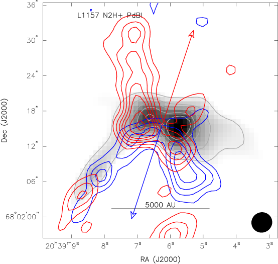
Figure 3: L1157– Maps of N₂H⁺ emission from the PdBI in L1157 in three velocity ranges; the blue and red lines denote the blue and red-shifted sides of the outflow (Jørgensen et al., 2007). The line-center emission from 2.33-3.1 km s^-1 is plotted as grayscale with light gray contours in units of 15, 30, 25, 60, 75$\sigma$ where $\sigma$=0.027 K km s^-1. The red contours are emission between 3.2 and 4 km s^-1 and the blue contours are emission between 1.57 and 2.2 km s^-1and plotted in units of 3, 6, 9, 12, 15, 21, 27$\sigma$. The red- and blue-shifted emission near the protostar is clearly shifted along the blue-shifted side of the outflow and both the blue and red-shifted emission seem to outline the outflow cavity wall. The spatial shifts along the outflow in the blue and red-shifted emission strongly suggest that the outflow is entraining material from the inner envelope.

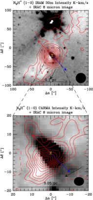
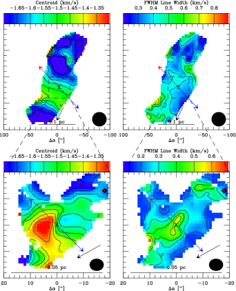
Figure 4: L1165– Same as Figure 1 but with CARMA data in the bottom row. The IRAM 30m contours start at 5$\sigma$ with 5$\sigma$ intervals; the CARMA data start at $\pm$3$\sigma$ with 3$\sigma$ intervals. The single-dish data show that the cloud has a fairly constant velocity away from the protostar, but near the protostar the kinematic structure is distinct; however, the single-dish linewidth map shows no indication of enhancement near the protostar. The velocity field from the interferometer map shows considerable detail, with a velocity gradient across the protostar nearly normal to the outflow. There is also enhanced linewidth near the protostar in the central envelope. Reference positions for the observations are listed in Tables 2 - 5.

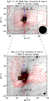
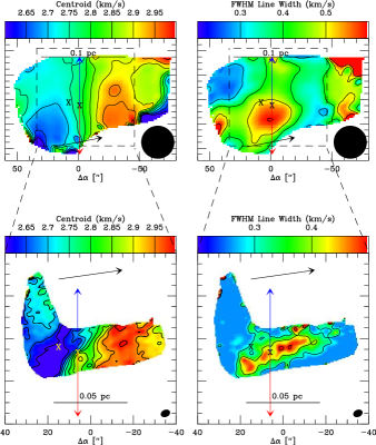
Figure 6: CB230– Same as Figure 1, but the interferometer data are VLA NH₃ (1,1) observations. The IRAM 30m contours start at 3$\sigma$ with 10$\sigma$ intervals; the VLA data start at $\pm$3$\sigma$ with 3$\sigma$ intervals. The line-center velocity from the single-dish data traces a fairly smooth velocity gradient across the envelope with enhanced linewidth near the protostar. The NH₃ intensity is less extended directly east of the protostar associated with the cutoff of 8$\mu$m extinction, the rest of the envelope appears fairly flat. The line-center velocity from the NH₃ emission traces a velocity gradient similar to the single-dish data; however, the shift from red to blue-shifted emission is quite abrupt and the transition region itself is curved. The NH₃ line-width does not show much detail other than having its peak coincident with the highest intensity NH₃ emission.

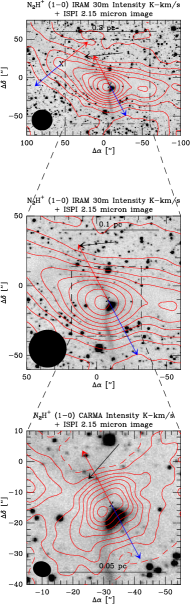
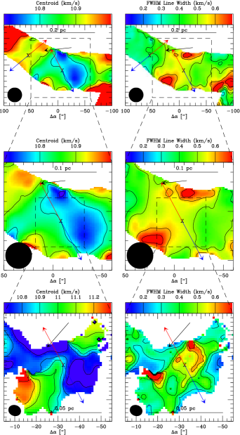
Figure 7: HH108IRS– Same as Figure 4, but zooming in on the single-dish data in the middle row and then the interferometer data in the bottom row. The IRAM 30m contours start at 3$\sigma$ with 10$\sigma$ intervals; the CARMA data start at $\pm$3$\sigma$ with 6$\sigma$ intervals. The N₂H⁺ peak in this object appears offset from the protostar in the single-dish and interferometer map. The interferometer map further appears to be elongated normal to the outflow. The single-dish line-center velocity map appears to show a slight gradient normal to the outflow, but the interferometric velocity field starts red-shifted, becomes blue-shifted and then goes back to red-shifted. The single-dish linewidth maps show a slight enhancement near the protostar; the interferometer data on the other hand show a highly increased linewidth near the protostar as compared to the surrounding region.

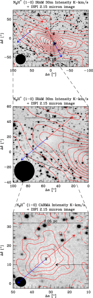
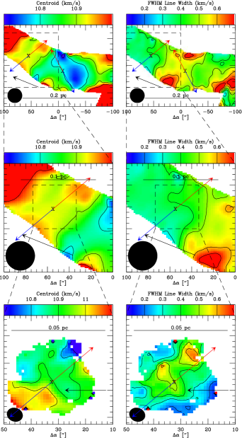
Figure 8: HH108MMS– Same as Figure 7. The IRAM 30m contours start at 3$\sigma$ with 10$\sigma$ intervals; the CARMA data start at $\pm$3$\sigma$ with 3$\sigma$ intervals. The single-dish integrated intensity map shows HH108MMS as an extension along a large-scale filamentary structure that connects with HH108IRS. However, the interferometer map finds the N₂H⁺ peak directly coincident with the protostar. The single-dish velocity field is fairly constant throughout the region of the envelope, but the large scale gradient is normal to its outflow. The CARMA velocity map then shows that there is a gradient along the outflow and the linewidth map shows increased linewidth along the outflow, this detail was absent in the single-dish map.

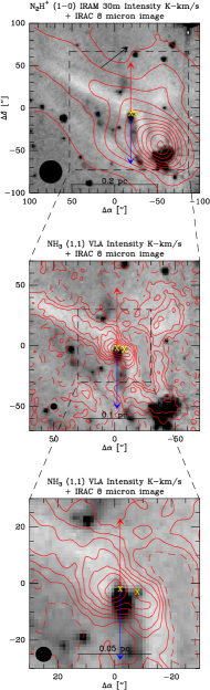
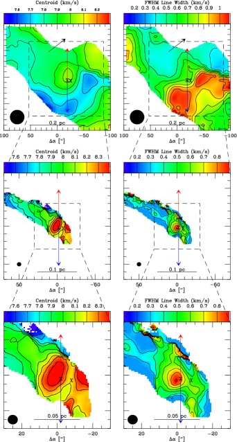
Figure 9: Serpens MMS3– Same as Figure 1 but with VLA NH₃ (1,1) data and an additional zoom-in of the NH₃ data in the bottom row. The IRAM 30m contours start at 5$\sigma$ with 10$\sigma$ intervals; the VLA data start at $\pm$3$\sigma$ with 5$\sigma$ intervals. The N₂H⁺ peak in the single-dish data is not on Serpens MMS3 but rather near a small cluster of young stars to the southwest, but there is an extension toward MMS3. The single-dish velocity field near MMS3 shows a red-shifted pocket associated with its position with a gradient extending along the direction of the large-scale filament shown in the top panels. The VLA NH₃ map reveals more detail as the emission closely follows the filamentary structures in the region. The NH₃ velocity map also shows the deep red-shifted pocket of emission next to the protostar and reveals more detail in the gradient along the filament. There is a corresponding increase in linewidth to the east of the protostar at the location of the red-shifted emission.

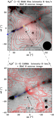
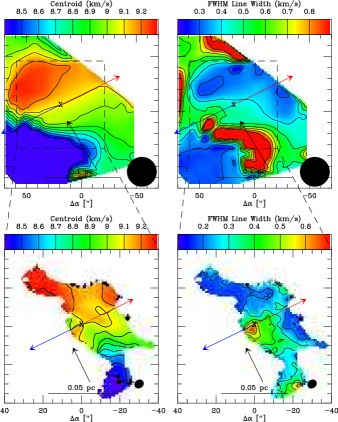
Figure 10: HH211– Same as Figure 4. The IRAM 30m contours start at 3$\sigma$ with 10$\sigma$ intervals; the CARMA data start at $\pm$3$\sigma$ with 3$\sigma$ intervals. As shown in the left panels, the N₂H⁺ emission mapped by the 30m and CARMA correlates very well with the 8$\mu$m extinction in the region. We also notice that the N₂H⁺ peak is offset from the protostar to the southwest in the single-dish and interferometer data. The velocity field shows a linear gradient normal to the outflow of HH211; however, south of the protostar there is another N₂H⁺ velocity component blue-shifted from the rest of the gas in the region. Tanner & Arce (2011) referred to this as the southwest extension. This transition region appears as artificially large line-width in the top right panel. The velocity field in the CARMA data also shows the linear gradient with a slight increase in linewidth near the protostar.

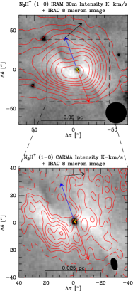
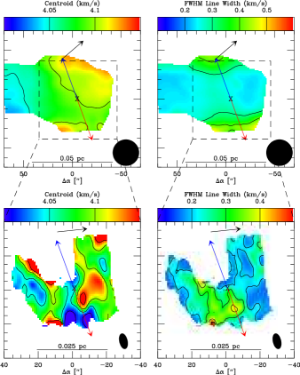
Figure 11: IRAS 16253-2429– Same as Figure 4. Both the IRAM 30m and CARMA contours start at 3$\sigma$ with 3$\sigma$ intervals. The single-dish N₂H⁺ emission traces the roughly symmetric envelope of IRAS 16253-2429 quite well with the peak emission just east of the protostar. The CARMA N₂H⁺ map also traces the envelope well and the northern outflow cavity is prominent as an evacuated region, probably due to resolved-out emission. The single-dish velocity field shows a very small velocity gradient roughly normal to the outflow. The CARMA velocity map shows complex structure, but there is an overall gradient in the same direction as the single-dish map. In addition, there is a red-shifted feature at the same location of as the outflow cavity wall. The single-dish and interferometer linewidth maps show slight enhancements at the same locations, where the peak emission is present, but there also is a linewidth increase toward the edge of the envelope along the outflow in the single-dish map. Note that the linewidth in the envelope is extremely narrow, only $\sim$0.2 km s^-1 over the regions where the outflow could not be interacting.

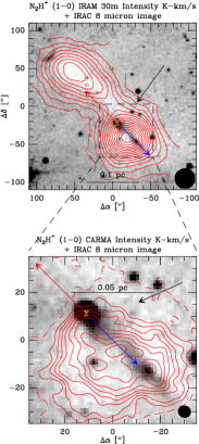
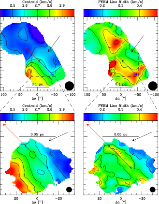
Figure 12: L1152– Same as Figure 4. The IRAM 30m contours start at 10$\sigma$ with 10$\sigma$ intervals; the CARMA data start at $\pm$3$\sigma$ with 3$\sigma$ intervals. The single-dish N₂H⁺ emission traces two connected peaks over $\sim$0.1 pc; one is star-less the other is adjacent to the protostar. The CARMA N₂H⁺ map focuses on the protostellar clump and clearly shows that the protostar is offset from most of the N₂H⁺ emission. Both velocity maps show a strong gradient normal to the outflow, while the star-less clump does not have much velocity structure. The linewidth maps show increases along the outflow; there is a feature in the single-dish map which is not exactly along the outflow but quite near it. The CARMA linewidth map shows increased linewidth that correlates very strongly with the jet-like emission shown in the 8$\mu$m image.

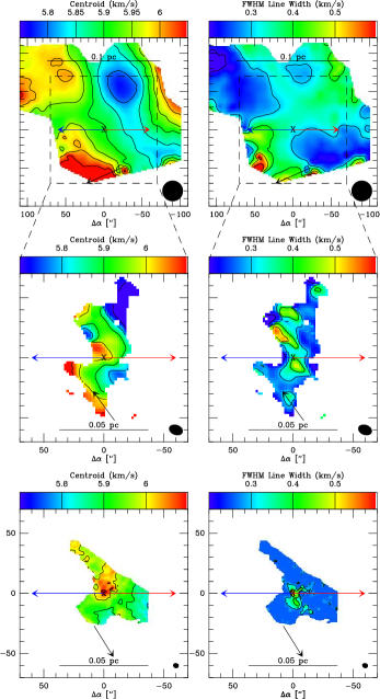
Figure 13: L1527– Same as Figure 4, but VLA NH₃ data are also shown in the bottom row. The IRAM 30m contours start at 5$\sigma$ with 10$\sigma$ intervals; both the CARMA and VLA contours start at $\pm$3$\sigma$ with 3$\sigma$ intervals. We show the NH₃ as well since they have slightly better resolution and because the N₂H⁺ data only have moderate signal-to-noise. The single-dish N₂H⁺ data are peaked north of the protostar, which is also the case for the CARMA data, but the VLA data are peaked south of the protostar. Both the VLA and CARMA data seem to trace a structure curving to the northeast which may be associated with the outflow cavity. The single-dish velocity field appears to have a component along the outflow and normal to it. The interferometer velocity maps reflect the single-dish velocities on the largest scales, but near the protostar there is a small-scale velocity gradient in the opposite direction of the large-scale gradient. There is little increase in linewidth in the single-dish data, but there appears to be increased linewidth near the protostar in both sets of interferometer data.

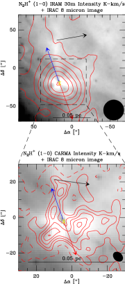
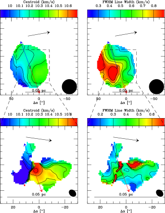
Figure 14: RNO43– Same as Figure 4. The IRAM 30m contours start at 3$\sigma$ with 10$\sigma$ intervals; the CARMA contours start at $\pm$3$\sigma$ with 3$\sigma$ intervals. The single-dish intensity map appears mostly unresolved, while the CARMA data trace the 8$\mu$m extinction structures closely with a depression of emission coincident with the protostar. The single-dish velocity field shows a gradient mostly normal to the outflow and the interferometer data reveal a sharp velocity shift between the east and west sides of the envelope. This appears as a line of broad linewidth (an artifact from fitting) where the two components are viewed on top of each other; this is associated with a region of large linewidth in the single-dish map.

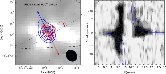
Figure 15: RNO43– Same as Figure 5. The contours levels are $\pm$5, 8, 11, 14, and 17$\sigma$ ($\sigma$ = 0.12 K) for the red and blue-shifted emission. The emission morphology of the HCO⁺ in both the integrated intensity map on the left and in the PV plot are quite similar to L1165. The total velocity extent of $\sim\pm$2 km s^-1 is similar in magnitude to L1165. However, the red and blue peaks are much closer together due to the increased distance of RNO43. The PV plot contours start at 3$\sigma$ and increase in 3$\sigma$ intervals ($\sigma$=0.2671). The solid-blue curve represents Keplerian rotation (or infall) for a 0.67 $M_{\sun}$ central object and the dashed-blue curve is for a 2.67 $M_{\sun}$ central object.

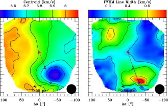
Figure 16: IRAS 04325+2402– Same as Figure 1, but we only have single-dish data for this object. The IRAM 30m contours start at 10$\sigma$ with 10$\sigma$ intervals. The N₂H⁺ contours correlate very well with the 8$\mu$m extinction and the peak is actually on an apparent star-less core north of the protostar. There is a tail of emission wrapping towards the protostar, but at lower intensity levels. The velocity field shows a gradient roughly normal to the outflow and there appears to be smaller-scale structure in the velocities near the protostar. The linewidth map does not show a large increase near the protostar but shows two peaks that are located along the outflow indicating a possible interaction.

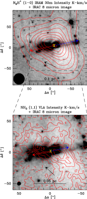
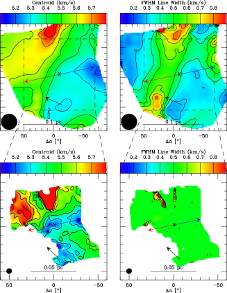
Figure 17: L483– Same as Figure 6, using archival NH₃ data from Fuller & Wootten (2000). The IRAM 30m contours start at 20$\sigma$ with 20$\sigma$ intervals; the VLA contours start at $\pm$3$\sigma$ with 6$\sigma$ intervals. The N₂H⁺ and NH₃ emission trace the envelope seen in 8$\mu$m extinction quite closely. The velocity field shows a gradient that is at an angle 45^∘ from the outflow in the single-dish map. The VLA velocity map shows a similar large-scale feature but there is a pocket of blue-shifted gas coincident with the protostar and there is a red-shifted pocket directly north of the protostar. The single-dish linewidth map shows increased linewidth at the location of the most rapid velocity changes; the VLA linewidth map only shows a couple of features where there is a sharp transition in the velocity components. This is due to only having 0.3 km s^-1 channel width in the NH₃ data.

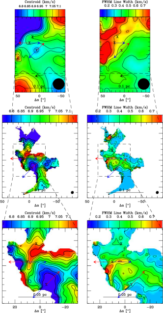
Figure 18: L673– Same as Figure 6 with an additional zoom-in on the NH₃ data in the bottom row. The IRAM 30m contours start at 20$\sigma$ with 20$\sigma$ intervals; the VLA contours start at $\pm$3$\sigma$ with 6$\sigma$ intervals. Though only three protostars are marked; there are likely seven in the region (Tsitali et al., 2010); the southern-most protostar marked is actually composed of three sources in Ks-band imaging (Tobin et al. in prep.). The single-dish N₂H⁺ emission fills the map, but there is increased emission where the 8$\mu$m extinction is most prominent. The NH₃ map only picks up the densest regions around the protostars. There is a gradient in the velocity map along the filament, though there appears to be features associated with the two marked protostars in both the single-dish and VLA maps. Both velocity maps also show a second velocity component to the north. The linewidth maps show increased linewidth at the transition region between the two components and the VLA map shows increased linewidth near the protostars.

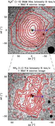
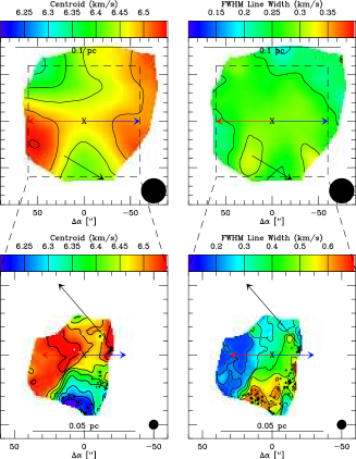
Figure 19: L1521F– Same as Figure 6. The IRAM 30m contours start at 3$\sigma$ with 3$\sigma$ intervals; the VLA contours start at $\pm$3$\sigma$ with 3$\sigma$ intervals. The single-dish data trace the region of 8$\mu$m extinction well and the NH₃ data trace the inner, high density regions. The velocity structure from the single-dish map shows weak evidence for a gradient normal to the outflow. The NH₃ data do show a gradient, but the emission near the protostar is all red-shifted and the blue-shifted emission is far (10″  1400 AU) from the protostar. However, as noted in the text, the NH₃ emission is optically thick and may not fully trace the inner envelope kinematics. The single-dish linewidth map has very little structure while the NH₃ linewidths are peaked coincident with the blue-shifted area of the velocity field.

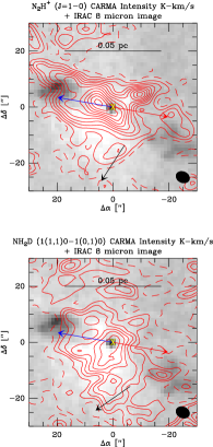
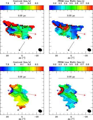
Figure 20: Perseus 5– The top row shows the CARMA N₂H⁺ ($J=1\rightarrow 0$) data and the bottom row shows the NH₂D ($1_{1,1}\rightarrow 1_{0,1}$) data also from CARMA; the contours start at $\pm$3$\sigma$ with 6$\sigma$ intervals for N₂H⁺ and $\pm$3$\sigma$ with 3$\sigma$ intervals for NH₂D. Both molecules have approximately the same noise level. The integrated intensity data for both molecules are overlaid on the IRAC 8$\mu$m images. NH₂D appears to trace the 8$\mu$m extinction best while N₂H⁺ is centrally peaked. The line-center velocity of each molecular line is shown in the center column, N₂H⁺ and NH₂D indicate that there may be a gradient normal to the outflow, but that there is also a gradient in the direction of the outflow. The linewidth plots in the right panels are complex, all show an enhancement away from the protostar along the outflow; NH₂D in particular shows an increase through the envelope near the outflow axis.

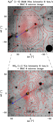
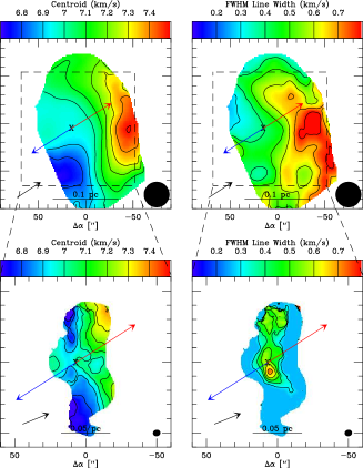
Figure 21: IRAS 03282+3035– Same as Figure 6. The IRAM 30m contours start at 3$\sigma$ with 10$\sigma$ intervals; the VLA contours start at $\pm$3$\sigma$ with 5$\sigma$ intervals. The single-dish N₂H⁺ emission closely traces the entire area viewed in 8$\mu$m extinction, peaking near the protostar. The VLA NH₃ data are picking up the densest region near the protostar. The velocity gradient is mostly along the outflow in the single-dish and VLA NH₃ velocity map. The linewidth in the single-dish data peaks to the west of the protostar, somewhat along the outflow. The NH₃ linewidth map has peaks about the protostar, normal to the outflow, and directly north, while the rest of the map has a small linewidth.

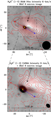
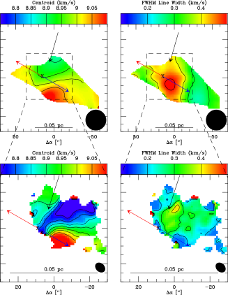
Figure 23: HH270 VLA1– Same as Figure 4. The IRAM 30m contours start at 3$\sigma$ with 6$\sigma$ intervals; the CARMA contours start at $\pm$3$\sigma$ with 3$\sigma$ intervals. The single-dish map shows strong emission coincident with the 8$\mu$m extinction extended along the outflow. The CARMA N₂H⁺ map shows a similar morphology, with no emission coincident with the protostar. The single-dish velocity field shows a gradient normal to and along the outflow; however, the CARMA velocity map shows that the gas velocity is relatively constant normal to the outflow, but along the outflow axis there is a clear gradient with more red-shifted emissions toward the outflow axis. The velocity contours trace a similar shape as the outflow cavity; the faint scattered light of the outflow cavity can be seen in the 8$\mu$m image. The single-dish linewidth map shows a peak along the outflow southwest of the protostar, this appears to be the unresolved velocity gradient along the outflow as the CARMA map does not have increased linewidth along at the same location.

We have computed velocity gradients for all objects using both the single-dish and interferometer data with the methods described in Section 2.6.2. The velocity gradients calculated from the single-dish data are given in Table 9 and the interferometric (N₂H⁺ and NH₃) velocity gradients are listed in Table 10. The gradient directions from the 2D fitting are plotted in Figures 1-23 and also listed in Tables 9 and 10. The one-dimensional (1D) cuts through the velocity fields, normal to the outflow and across equatorial plane of each envelope, are shown in Figure 24 presenting an alternative view of the envelope velocity structure. Linear fits to the single-dish and interferometer data are overlaid on the plots. Notice that in some cases the velocity of the interferometer data diverges from the single-dish data. This results from the interferometer filtering-out larger-scale emission that dominated the single-dish data and the increased resolution picking out smaller-scale velocity structure.

The gradients calculated for the single-dish data with each method are comparable. The median single-dish velocity gradients from the different fitting methods are: 2.1 km s^-1 pc^-1  (1D fitting), 1.7 km s^-1 pc^-1  (1D two points), and 2.2 km s^-1 pc^-1  (2D fitting); the mean gradients are 2.3, 2.2, and 2.04 km s^-1 pc^-1  respectively. The distribution of single-dish velocity gradients from the three methods is shown in Figure 25. The lower values of the two point method reflect that the region inside the 10000 AU radius of some sources has a higher velocity gradient; there are velocity decreases toward the edges of some envelopes that are reflected in the plots in Figure 24, yielding a preference toward lower gradients in Figure 25.

The mean velocity gradient of the single-dish sample ($\sim$2.2 km s^-1 pc^-1 ) is about twice the average gradient in Goodman et al. (1993) and slightly higher than Caselli et al. (2002), but our sample of 16 objects is smaller than their larger samples. We can expect to observe larger velocity gradients with our higher resolution data because the lower resolution data in Goodman et al. (1993) and Caselli et al. (2002) tend to smear velocity components together. L483 was common between our work and the two previous studies, with very similar gradient magnitudes and PAs. L1527 and L1152 were also common between our work and Goodman et al. (1993). The gradient directions fit for these sources were similar, but the magnitude of the gradients are different. We regard our values as being more reliable because our maps are comprised of substantially more independent points.

The interferometric sample has a median velocity gradient of 8.1 km s^-1 pc^-1  from 2D fitting and 10.7 km s^-1 pc^-1  from 1D fitting, both having a mean gradient of 8.6 km s^-1 pc^-1 . The distribution of interferometric velocity gradients from the two methods is shown in Figure 26. The interferometric gradients are often larger than the single-dish gradients by factors of several. The 2D fitting method was less reliable for the interferometric data given the often complex velocity fields present within the data. Reliable 2D fits could not be obtained for L1157 (PdBI data) or Serpens MMS3 due to lack of convergence on their complex velocity fields. Our range of observed velocity gradients is comparable to what Chen et al. (2007) found; however, they found three protostellar systems with gradients $>$20 km s^-1 pc^-1 , we do not find such large gradients in our data.

Using the outflow PAs derived from the Spitzer imaging and CO data from the literature, we have compared the gradient PAs (the angle toward increasing velocities) with the outflow PAs in Figure 27. The gradient position angles are also marked in Figures 1-23 with solid arrow; the majority of the velocity gradients are within 45° of normal to the outflow. The distribution of interferometric velocity directions strongly shows a trend for being oriented normal to the outflow axis. The gradient directions also generally reflect what is seen at large-scales in the single-dish data. Table 10 and Figure 28 show that only three systems have velocity gradient directions which differ by more than 45° between the single-dish and interferometric measurements.

The majority of envelopes in the interferometric sample have an ordered velocity structure, despite their often complex morphological structure. In contrast to Volgenau et al. (2006) and Chen et al. (2007), many systems have velocity gradients roughly normal to the outflow direction, this likely results from our larger sample of observations as compared to the Chen et al. (2007) and especially Volgenau et al. (2006). In addition, visual inspection of the data shows that the large and small-scale velocity gradient directions are generally consistent with one another, a feature which Volgenau et al. (2006) also sees in their sample. The interferometer observations often reveal small-scale kinematic detail near the protostar that is smeared-out in the lower-resolution single-dish data.

3.3 Description of Individual Sources

We will describe the dataset for each source individually in the following subsections and the discuss of our results as a whole is in Section 4.

3.3.1 L1157

The flattened, filamentary envelope of L1157 has been extensively studied in recent years (e.g. Looney et al., 2007; Chiang et al., 2010, Paper I). Its velocity field was first studied in Chiang et al. (2010), which showed a weak velocity gradient along the filament, normal to the outflow. We subsequently observed L1157 with the IRAM 30m, the PdBI, and the VLA. Figure 1 shows the data from the IRAM 30m and PdBI and Figure 2 shows the data from the VLA and CARMA. The 30m data detects a large-scale velocity gradient normal to the outflow and this gradient follows the long axis of the envelope. On the east side of the envelope, where the emission curves downward, the N₂H⁺ continues to trace dense material as it becomes more blue-shifted.

The PdBI data are shown in the bottom panels of Figure 1. The N₂H⁺ emission appears double-peaked on small-scales. The 3mm dust continuum shows that the protostar resides between the peaks (see Appendix); the peaks are at radii of $\sim$1000 AU ($\sim$3.5″). The velocity field on scales $>$15″ reflects what has been seen with the CARMA, 30m, and VLA data. On the other hand, the velocity of the gas becomes highly red-shifted ($\sim$1 km s^-1) at the N₂H⁺ peaks as compared to the surrounding gas at $\sim$1000 AU from the protostar. The high-velocity gas was observed in Chiang et al. (2010); however, its spatial location was not well-resolved in the CARMA data due to having a factor of $\sim$2 lower resolution than the PdBI data. Note that the 2D velocity gradient fits for the VLA and CARMA data have position angles that differ by 80°. This results from the north-south gradient being more prominent in the CARMA N₂H⁺ data while the east-west gradient appears more prominent in the NH₃ data. A 2D gradient could not be fit to the PdBI data due to the highly complex velocity field present on small-scales.

The single-dish velocity and linewidth maps show a gradual large-scale velocity gradient in L1157 with broad linewidth in the inner envelope, consistent with the PdBI linewidth map in Figure 1. The broad linewidths were also shown in lower resolution data from Chiang et al. (2010). Both the east and west peaks in the PdBI maps have velocity wings toward the red and are not significantly extended toward blue-shifted velocities. Chiang et al. (2010) attributed the broad inner envelope line wings to infall. However, close examination of our higher-resolution PdBI data indicate that the blue and red-shifted line wings may result from outflow interaction effects. Figure 3 shows that the most red-shifted emission is slightly shifted to the southeast, along the outflow and traces one edge of the northern outflow cavity. Furthermore, the blue-shifted emission also seems to outline the southern outflow cavity quite well. Thus, it appears that the outflow is may be entraining inner envelope material, while at larger scales the velocity structure appears unaffected by the outflow, tracing the intrinsic kinematic structure of the envelope. The spatial overlap of red and blue-shifted N₂H⁺ southeast of the protostar on the blue-shifted side of the outflow can understood if the outflow is entraining material within a symmetric cavity in the inner envelope, producing both a blue and red-shifted component. There also appear to be outflow effects in the N₂H⁺ emission on the northwest side of the protostar but to a lesser extent. This is the first example of possible outflow entrainment in such a dense gas tracer. However, we note that rather than entrainment, the broad N₂H⁺ emission could also result from an outflow shock at that location.

3.3.2 L1165

The protostar L1165IRS is located within a $\sim$1.5 pc (17′) long filamentary dark cloud (Paper I). The narrow filament, from which the protostar has formed, is normal to the protostellar outflow. We mapped a 4^′ section of the dark cloud surrounding the protostar, as shown in the left panels of Figure 4. The N₂H⁺ emission is highly peaked very near the protostar, it is slightly offset 4.87″($\sim$1462 AU) to the southeast, and there is low-level extended emission associated with regions of 8$\mu$m extinction. The velocity field from the single-dish N₂H⁺ data shows a fairly linear gradient nearly normal to the outflow; in areas away from the protostar the filament generally seems to have a fairly constant velocity with little variation and small linewidth.

The N₂H⁺ data from CARMA reveal a small-scale structure that is extended in the direction of the filament axis and the emission is strongly correlated with the small-scale 8$\mu$m extinction shown in Figure 4. At the edges of detected emission, the velocity field of the interferometer map is consistent with the single-dish data. However, near the protostar there is a 0.35 km/s velocity shift between the blue and red-shifted velocity peaks that are on opposite sides of the protostar. We note that this velocity gradient is not perfectly normal to the outflow, but rather offset by about $\sim$30^∘. However, the most red-shifted emission is slightly extended in the direction of the outflow, but the linewidth peak is extended normal to the outflow and the red-shifted emission at this location does not appear to be outflow affected. Thus, the gradient from the envelope itself appears to be normal to the outflow and tracing gravitationally dominated motion.

We show the HCO⁺ emission in Figure 5, in which the red and blue-shifted emission is confined to two clumps, that are oriented normal to the outflow and offset from the protostar by 3^′′. The position-velocity plot of these data show the blue and red-shifted emission extending $\sim$2 and $\sim$1.5 km s^-1 away from the systemic velocity respectively. Given the orientation of the blue and red-shifted emission normal to the outflow and a lack of emission along the outflow, the HCO⁺ emission appears to be originating from the inner envelope. Assuming that the HCO⁺ emission indicates rotationally supported motion, we can calculate the enclosed mass using $M=R\Delta v^{2}/G$ which gives M_enc $\sim$ 2.0$M_{\sun}$. This is not unreasonable for this source which has $L_{bol}$ $\sim$14$L_{\sun}$ assuming a distance of 300 pc. However, if the velocities result from equal contributions of rotation and infall, then the enclosed mass would be a more modest 0.5 $M_{\sun}$. We have overlaid lines representing Keplerian rotation (or infall) on Figure 5, the 0.5$M_{\sun}$ curve matches the data much better than the 2.0$M_{\sun}$ curve.

3.3.3 CB230

CB230 is an isolated protostar that formed at one end of its natal globule (Paper I). This protostar was discovered to be a wide binary system by Yun (1996) with a separation of $\sim$10^′′, the companion is evident in the 8$\mu$m images shown in Figure 6. The envelope around CB230 was classified as a “one-sided” envelope in Paper I due to the 60^′′ (30000 AU) extension of the extinction envelope to the west, while the 8$\mu$m extinction terminates just $\sim$25^′′ (6000 AU) on the eastern side. The single-dish N₂H⁺ emission is consistent with the 8$\mu$m extinction observations, the emission falling off steeply to the east and more extended to the west. The large-scale extension of material beyond the region of detected N₂H⁺ emission suggests that it has lower density and has not formed N₂H⁺ at detectable levels, see Section 4.5 for further discussion.

The NH₃ emission from the VLA is strongest in a “bar,” about 10^∘ from normal to the outflow. Notably, at the location of the protostar there is a ”hole” in the ammonia emission; a similar depression of emission is seen in N₂H⁺ ($J=1\rightarrow 0$) by Chen et al. (2007) and Launhardt et al. (2001). The region of decreased emission is $\sim$2200AU in diameter, similar in size to the double-peaked N₂H⁺ emission in L1157. The lower level emission on the eastern side of the protostar extends northward along the outflow cavity. Incidentally, the northward extension is also where the scattered light emission in the near-IR and Spitzer 3.6$\mu$m is brightest (Paper I; Launhardt et al., 2010).

The velocity field of the single-dish N₂H⁺ shows a fairly linear gradient, normal to the outflow, with a “plateau” of the most highly red/blue-shifted emission $\pm$30^′′ from the protostar. South of the protostar, the N₂H⁺ linewidth peaks, similar to L1157. The NH₃ velocity gradient from the VLA data is in the same direction as the single-dish gradient and similar to the interferometric N₂H⁺ map from Chen et al. (2007). While the single-dish gradient is fairly gradual, the gradient from the VLA observations has an abrupt shift from blue to red-shifted emission coincident with the protostar. The VLA NH₃ data also show a velocity “plateau” in the blue and red-shifted emission, with the highest relative-velocity emission being $\pm$15^′′ from the protostar. The linewidth remains fairly constant throughout the regions near the protostar, peaking at 0.5 km/s. The region of highest linewidth also corresponds to the region of strongest ammonia emission. The large linewidth seen near the protostar in the single-dish data is not reflected in these NH₃ data nor the N₂H⁺ data of Chen et al. (2007). The line-center velocity changes quite rapidly at the location of the large single-dish linewidth; therefore, the linewidth peak is likely due to the unresolved velocity gradient. This means that the outflow is not likely to be affecting the kinematics of the inner envelope in this protostar.

3.3.4 HH108IRS

The protostar HH108IRS, the driving source of HH108, is located within a large-scale filament, $\sim$0.5 pc in length, 1.75^∘ south of the Serpens star forming region (Harvey et al., 2006). There are at least two protostars forming in the filament: the higher luminosity object HH108IRS and the deeply embedded source HH108MMS (Chini et al., 2001). The single-dish N₂H⁺ map in Figure 7 shows an emission peak coincident with HH108IRS,but slightly offset from the protostar $\sim$5″ (1500 AU). The N₂H⁺ map from CARMA reveals that the N₂H⁺ peak emission is truly offset from the protostar and emission is extended normal to the outflow direction, forming a flattened structure across the protostar.

The single-dish N₂H⁺ velocity map indicates that there may be a slight gradient normal to the outflow. The CARMA N₂H⁺ velocity map reveals that there is indeed a velocity gradient normal to the outflow, though its structure is complex. Southeast of the protostar the velocities are red-shifted and moving toward the protostar the velocities are becoming more blue-shifted. This trend continues after crossing the protostar and moving northwest, but then the trend reverses itself rapidly and becomes more red-shifted. We also note that the linewidth is $\sim$0.6 km/s within $\pm$10^′′ (3000 AU) around the protostar, indicative of a dynamic environment near the protostar. The single-dish linewidth is consistent with this value as well.

3.3.5 HH108MMS

HH108MMS is the nearby neighbor to HH108IRS, separated by $\sim$60″ ($\sim$0.09 pc). This protostar is deeply embedded and invisible at 24$\mu$m, only becoming visible at 70$\mu$m (Paper I). There are no IRAC data available for this object, therefore we are showing an ISPI Ks-band (2.15$\mu$m) image from Paper I. Despite the lack of 8$\mu$m extinction observations, we can clearly see the dense material of the envelope blocking out the rich background star field. The single-dish N₂H⁺ in Figure 8 shows a slight extension toward the location of the protostar (derived from 70$\mu$m and 3mm continuum), while the CARMA N₂H⁺ observations clearly show the N₂H⁺ emission centrally peaked on the protostar.

The single-dish velocity field does not show much structure, the region within $\pm$30″ (0.045 pc) of the protostar has a roughly constant velocity. The filament that HH108MMS is forming within has a velocity gradient of 1.6 km s^-1 pc^-1  running from southwest to northeast. The CARMA N₂H⁺ velocity map on the other hand shows significant structure on $\sim$10″ scales within $\pm$15″ ($\sim$0.02 pc) of the protostar. Southeast of the protostar the emission is red-shifted and northwest there is blue-shifted emission, along the presumptive outflow axis and HCN emission mapped with CARMA (Tobin et al. 2011 in preparation). The outflow axis is determined from faint diffuse emission seen in Ks-band. The CARMA map also shows increased linewidth along the outflow; there is no indication of such an increase in the single-dish map, likely due to beam dilution. HH108MMS appears to be a prime example of the outflow impacting the envelope of a deeply embedded protostar.

3.3.6 Serpens MMS3

Serpens MMS3 is located within a complex network of filamentary structure in the Serpens B cluster (Djupvik et al., 2006; Harvey et al., 2006), shown in Figure 9. One of the most prominent filaments runs $\sim$0.1 pc in length into Serpens MMS3, see left panels of Figure 9. Directly west of the protostar the filament turns southward toward a small clustering of bright young stars. We also noticed that Serpens MMS3 has a faint companion separated by $\sim$7^′′.

The single-dish N₂H⁺ map shows that the emission is highly pervasive throughout the region. The emission is peaked near the clustering of young stars in the southwest corner of the image in Figure 9. However, the emission is extended toward Serpens MMS3 and there is enhancement emission coincident with the large scale filament seen in 8$\mu$m extinction. The VLA NH₃ map reveals the structure of the region in substantially more detail. The interferometer resolved out whatever diffuse NH₃ emission was in the region and the remaining emission directly correlates to the highest extinction regions seen in the 8$\mu$m image, with a peak coincident with the Serpens MMS3 protostar. The NH₃ emission is still extended toward the clustering of young stars in the southwest, but it is at the edge of the primary beam.

The overall velocity structure of this region is confusing in the single-dish N₂H⁺ velocity map because of the multitude of high-density structures in the region; however, there is a large scale gradient along the filament that Serpens MMS3 resides in and there is also a pocket of red-shifted emission next to the protostar. The VLA NH₃ (1,1) map also shows this large scale gradient along the filament of Serpens MMS3 and red-shifted emission next to the protostar. The red-shifted emission appears over a region 15″ from the protostar and is extended in the direction of the outflow. We also detected an increased linewidth ($\sim$1 km s^-1) next to the protostar. Directly southwest of the protostar the velocity gradient appears to resume the large-scale velocity trend exhibited northeast of the protostar. It is presently unclear if the kinematic structure near the protostar is related to the outflow or infall, but its proximity and extension along the outflow makes us suspicious. However, the broad linewidth is quite localized to the east of the protostar.

3.3.7 HH211

HH211MMS is a deeply embedded protostar on the outskirts of the IC348 cluster in the Perseus molecular cloud; emission from the central protostar itself only becomes evident at 70$\mu$m (Rebull et al., 2007) and has been found to be a proto-binary in the submillimeter (Lee et al., 2009). We see a large absorbing structure in the 8$\mu$m extinction map shown in Figure 10, as well as its powerful outflow (McCaughrean et al., 1994; Gueth & Guilloteau, 1999). The single-dish N₂H⁺ emission associated with HH211MMS is very strong, peaked to the southwest of the protostar itself. The N₂H⁺ emission also appears extended in the direction of the higher extinction areas. The N₂H⁺ emission mapped with CARMA detects emission on small scales around the protostar, with the emission peak offset $\sim$2^′′ southwest of the protostar (not coincident with the single-dish N₂H⁺ peaks). The emission is more extended along the northwestern side of the outflow, consistent with the extinction seen in the 8$\mu$m image.

The single-dish N₂H⁺ velocity map shows a linear velocity gradient normal to the outflow and south of the protostar there is another velocity component in the dense gas. The transition between these two velocity components appears as an area of artificially large linewidth (an artifact from fitting); however, there are two sets of narrow emission lines present, not broad lines. The CARMA N₂H⁺ velocity map also finds a linear gradient normal to the outflow as well as the second velocity component to the south. We also note that near the protostar the gradient is not perfectly linear at all scales. The deviance from a linear gradient is slight; however, it is present where we also have excellent signal-to-noise and this agrees with the velocity map by Tanner & Arce (2011).

The linewidths in the single-dish data were quite low across the source, only 0.3 - 0.4 km s^-1 with similar levels seen in the CARMA N₂H⁺ map. We note that there is an area of increased linewidth just southeast of the protostar, apparently at the base of the outflow. We suggest that the increased linewidth in this region is due to outflow interaction, in agreement with Tanner & Arce (2011). In addition, the filament northeast of the protostar has a very narrow linewidth, $<$0.2 km s^-1, appearing both the single-dish and interferometer maps.

3.3.8 IRAS 16253-2429

IRAS 16253-2429 is a low-luminosity ($L_{Bol}=0.25L_{\sun}$) Class 0 protostar in the $\rho$ Ophiuchus star forming region; it is also identified as Oph MMS 126 (Stanke et al., 2006). We noted in Paper I that this was one of the more “symmetric” envelopes seen in our 8$\mu$m extinction study. Its symmetric bipolar outflow has been traced in CO by Stanke et al. (2006) as well as in shocked H₂ emission from Spitzer IRS spectral mapping (Barsony et al., 2010).

The single-dish N₂H⁺ shown in Figure 11 correlates quite well with the 8$\mu$m extinction. The emission peak is slightly offset from the location of the protostar and the N₂H⁺ emission appears to be depressed at the location of the outflow cavities. The CARMA N₂H⁺ emission shows similar features in that it strongly correlates with the regions of 8$\mu$m extinction and there is less emission in regions occupied by the outflow cavities. The lack of emission within the outflow cavities is likely due to evacuation of envelope material and/or destruction of N₂H⁺ by CO in the outflow (section 4.2); there may also be some interferometric filtering-out of emission in this region. Furthermore, there appears to be a deficit of N₂H⁺ emission near the protostar.

The velocity field of the single-dish N₂H⁺ map indicates that there is a very small velocity gradient across the envelope, approximately normal to the outflow; note the small velocity range occupied by the envelope and velocity gradient. The velocity map from the CARMA N₂H⁺ data is more complex with several gradient reversals throughout the emitting region. However, the global gradient still seems to be present in interferometer data. Furthermore, a VLA NH₃ map shows a velocity structure very similar to our CARMA N₂H⁺ map (J. Wiseman, private communication).

The single-dish N₂H⁺ linewidth is quite small and constant across the envelope, whereas many other objects in our sample have linewidths which peak near the protostar. We also note that the linewidth is increasing in this source toward the edge of N₂H⁺ emission along the outflow; this is likely an outflow interaction effect. The CARMA N₂H⁺ map shows a similar small linewidth across the most of the envelope; however, there is a region of increased linewidth east and south of the protostar associated with an area of strong N₂H⁺ emission; at this location there is a slight enhancement of linewidth in the single-dish map.

3.3.9 L1152

The L1152 dark cloud is located in Cepheus, about 1.7 pc (20^′) away from L1157 on the sky. L1152 hosts three young stars; however, only one (IRAS 20353+6742) is classified as a Class 0 object and it is the only one embedded in the main core of L1152 (Chapman & Mundy, 2009). Paper I found that the main core of L1152 appears to have a “dumbbell” morphology in which the northeastern core (see Figure 12) appears to be starless and the southeastern core harbors IRAS 20353+6742 (hereafter L1152). These two concentrations are connected by what appears to be a thinner filament of high density material.

The single-dish N₂H⁺ ($J=1\rightarrow 0$) emission shown in Figure 12 exactly matches the morphology of the extinction in the 8$\mu$m images. However, the peak N₂H⁺ emission in the southwestern core is offset from the protostar by $\sim$20^′′ (6000 AU). The N₂H⁺ map from CARMA shown in the right panel of Figure 12 only observed the southeastern core. The map confirms that the N₂H⁺ is substantially offset from the protostar and there is no sub-peak at its location. However, the N₂H⁺ emission appears to extend toward the protostar.

The single-dish N₂H⁺ velocity field exhibits a velocity gradient normal to the outflow of L1152, noting that the protostar appears at the edge of the region exhibiting the gradient. The rest of the cloud, including the star-less core, has a fairly constant velocity; only varying by $\sim$ 0.1 km/s. However, we do notice increased linewidths northeast and southwest of the protostar. Southwest of the protostar we can clearly see the jet from the protostar, possibly interacting with envelope material, then in the northeast there is nothing obvious happening at this linewidth peak in the 8$\mu$m image. However, the northeast linewidth peak is near the outflow axis and this could be the cause of the increased linewidth at this location.

The velocity map from the CARMA N₂H⁺ data tells a remarkably similar story to the single-dish data; the velocity gradient is only slightly better resolved. However, the most remarkable feature is in the linewidth map, where we clearly see an increase in linewidth on the axis of the jet that is visible in the 8$\mu$m maps. This appears to be a another very clear example of the outflow interacting with the envelope material, though the velocity field does not seem to show outflow effects.

3.3.10 L1527

L1527 (IRAS 04368+2557) is an extensively studied protostar in Taurus. Benson & Myers (1989) observed its compact NH₃ core, from which Goodman et al. (1993) derived its velocity gradient. Subsequent observations indicated the possibility of infall in the envelope from H₂CO observations by Myers et al. (1995). Furthermore, detailed modeling of its scattered light cavities observed in Spitzer IRAC imaging have been done by Tobin et al. (2008) and Gramajo et al. (2010). High-resolution mid-infrared imaging by Tobin et al. (2010a) found the signature of a large (R$\sim$200 AU) disk in scattered light.

IRAC 8$\mu$m imaging of this source revealed an asymmetric distribution of extinction, the northern side of the envelope is substantially more extended than the southern side. This asymmetry is also exhibited in our single-dish N₂H⁺ shown in Figure 13; in addition, the peak emission is also offset to the north of the protostar by $\sim$25^′′ (3500 AU). The VLA NH₃ and CARMA N₂H⁺ maps both show emission associated with the protostar, but the maps are somewhat difficult to interpret due to the likelihood of spatial filtering. In addition, the CARMA observation was done as a mosaic in order to cover the entire region of emission as the primary beam is only 70^′′; both maps seem to detect emission in the same general areas.

The velocity field from the single-dish N₂H⁺ map has a complicated morphology. There appear to be two velocity gradients in the map, one along the outflow (pointed out by Myers et al. (1995)) and another normal to the outflow isolated by Goodman et al. (1993). However, the gradient along the outflow is not linear, the velocities go from red to blue and back to red. The linewidth remains fairly constant throughout the map, with a minimum at the northeast and southwest edges of the map.

The velocity fields from both the VLA and CARMA reveal further kinematic complexity in this system. We can see the consistency with the single-dish velocity map on large-scales; however, the N₂H⁺ and NH₃ maps show that there is a small-scale velocity gradient near the protostar. Notice that this small-scale velocity gradient is in the opposite direction as compared to the large-scale gradient. The linewidths of the N₂H⁺ and NH₃ exhibit a corresponding increase in the inner envelope, near these small-scale velocity gradients. This is the only protostellar envelope that where a velocity gradient reversal is seen going from large to small-scales.

3.3.11 RNO43

RNO43 is protostar forming within the $\lambda$ Ori ring. On large scales the envelope is quite asymmetric, with several filamentary structures appearing to converge at the location of the protostar as shown in the left panels of Figure 14. RNO43 also drives a powerful, parsec-scale outflow; CO emission has been mapped on small scales by Arce & Sargent (2005) tracing an outflow cavity and on large-scales, tracing a $\sim$5 pc long outflow (Bence et al., 1996). The N₂H⁺ emission is mostly unresolved in the single-dish map as shown in Figure 14. The peak emission is located near the location of the protostar and there are slight extensions in the direction of the outflow.

The CARMA N₂H⁺ ($J=1\rightarrow 0$) map traces the small-scale structure seen in 8$\mu$m extinction very well. We also note a depression of N₂H⁺ emission at the location of the protostar, consistent with observations of other protostars in our sample; see Section 4.5 for further discussion of this feature. East of the protostar there is a ridge of N₂H⁺ emission which is composed of the three bright knots almost running north-south in the image extending $\sim$35^′′. The southern-most knot is associated with the highest column density region east of the protostar and the two northern knots correlate well with an extinction filament running from the north into the envelope of RNO43. In addition, this filament of 8$\mu$m extinction and N₂H⁺ emission are coincident with the brightest part of the outflow cavity in the Spitzer 3.6$\mu$m image (Paper I). Directly west of the protostar, there is another peak of N₂H⁺ emission and weaker N₂H⁺ emission extended further west, in agreement with the 8$\mu$m extinction. Chen et al. (2007) mapped this region in N₂H⁺ using OVRO, the data agree quite well with our observations. However, our map appears to have recovered more large-scale emission, likely due to better uv-coverage at short spacings.

The velocity field from the single-dish N₂H⁺ map shows a large scale velocity gradient that is nearly normal to the outflow axis and there is an area of enhanced linewidth southeast of the protostar. The CARMA data reveal significant kinematic detail in the velocity field of the N₂H⁺ gas. The CARMA velocity maps in Figure 14 clearly show red and blue-shifted sides of the envelope; however, separating those sides of the envelope is a sharp velocity jump from blue to red by $\sim$0.7 km s^-1. Due to the overlapping lines at the location of the protostar, the N₂H⁺ linewidth forms a line marking the jump in velocity. There also appears to be a north-south gradient in the interferometer data as well (the single-dish map hints at this). Chen et al. (2007) ignored the western, red-shifted portion of the envelope thinking that it was a line-of-sight alignment with another clump; however, the envelope has density increasing in 8$\mu$m extinction toward the protostar on both sides (shown in Paper I), suggesting that the western side is indeed part of the same structure.

We note that the most highly blue-shifted gas is not located directly adjacent to the protostar; this is likely due to the absence of N₂H⁺ near the protostar, as mentioned earlier. Furthermore, small-scale emission of HCO⁺ was also detected with similar morphology to L1165 (Figure 5). Figure 15 shows that the centroid of blue and red-shifted emission are located normal to the outflow and are offset from each other by $\sim$3^′′ (1400 AU). In RNO43, the HCO⁺ line wings extend $\pm\sim$2 km/s from the systemic velocity. If we assume that the HCO⁺ emission reflects only rotation, its velocities would imply an enclosed mass of 2.7$M_{\sun}$. If only half of this velocity is due to rotation then the enclosed mass would be 0.67$M_{\sun}$. The bolometric luminosity of RNO43 is $\sim$8.0$L_{\sun}$; comparable to L1165 in both luminosity and mass. We have overlaid lines representing Keplerian rotation (or infall) on Figure 15, the 0.67$M_{\sun}$ curve matches the data much better that the 2.67$M_{\sun}$ curve.

Note that we have redefined the outflow position axis to be 20^∘ east of north in contrast to the 54^∘ found by Arce & Sargent (2005); our value is more accurate taking into account the outflow cavity observed by Spitzer (Figure 14) and CO maps from both Arce & Sargent (2005) and Bence et al. (1996). Furthermore, Chen et al. (2007) assumed the 54^∘ outflow position axis, leading them to interpret the velocity gradient along the eastern ridge as symmetric rotation. The N₂H⁺ gradient across the protostar has a very similar direction to the H¹³CO⁺ and C¹⁸O velocity gradients found by Arce & Sargent (2005). However, our revised outflow axis and the observed N₂H⁺ velocity structure, in conjunction with the H¹³CO⁺ and C¹⁸O data, lead us to suggest that we are likely not seeing envelope material being “pushed out” in this system, as suggested by Arce & Sargent (2005). Thus, the N₂H⁺ velocity structure appears to reflect kinematic structure intrinsic to the envelope.

3.3.12 IRAS 04325+2402

IRAS 04325+2402, sometimes referred to as L1535, harbors a multiple Class I protostellar system in the Taurus star forming region. The primary is possibly a sub-arcsecond binary with a wider companion separated by 8.2^′′ (Hartmann et al., 1999). The 8$\mu$m extinction around IRAS 04325 was found in our envelope study but not published in Paper I due to its low signal-to-noise; however, Scholz et al. (2010) noticed the 8$\mu$m extinction in their study of the system. These authors pointed out that there is a bright diffuse region of emission at 3.6 and 4.5$\mu$m, at the peak of the 8$\mu$m extinction. Furthermore, they noticed a dark band between the protostar and the 4.5$\mu$m diffuse emission, suggesting a dense cloud; however, there is a lack of 8$\mu$m extinction at the location of the dark band.

Our single-dish N₂H⁺ map finds emission throughout the core surrounding the protostar with the peak emission coincident with the 8$\mu$m extinction peak and the 4.5$\mu$m diffuse scattered light peak. In fact, the N₂H⁺ is peaked $\sim$60″ northeast of the protostar, but the map does show a slight enhancement of N₂H⁺ emission west of the protostar. Given this emission morphology, we suggest that the dark band see at 4.5$\mu$m is really just a lack of material and that the diffuse emission is light from the protostar shining onto the neighboring star-less core. We have no interferometry data for this object, however we would not expect to observe substantial N₂H⁺ emission peaked around the protostar, based on the single-dish map.

The velocity structure of the N₂H⁺ shows that there is a relatively smooth velocity gradient across the entire object with an increased gradient just southeast of the protostar. The linewidth of N₂H⁺ however shows large increase along the outflow axis of the protostar. Thus, the outflow from the protostar may be interacting with the dense material in the surrounding core producing the increased linewidth. On the other hand, the velocity field does not seem to show effects from the outflow, similar to L1152.

3.3.13 L483

L483 is an isolated globule harboring a Class 0 protostar (Tafalla et al., 2000). The envelope surrounding the protostar is quite large, $\sim$0.15 pc in diameter with at least 10-20$M_{\sun}$ of material measured from 8$\mu$m extinction in Paper I. The densest regions seen in 8$\mu$m extinction form a “tri-lobed” pattern that is also traced by 850$\mu$m emission (Jørgensen, 2004). The single-dish N₂H⁺ also follows this same pattern with the peak emission coincident with the protostar, see Figure 17. The VLA NH₃ emission is not peaked on the protostar, but also follows the ”tri-lobed” morphology. The N₂H⁺ emission mapped with OVRO by Jørgensen (2004) is extended along the outflow; however, this observation appears to have resolved out a significant amount of extended emission.

The velocity gradient from the single-dish N₂H⁺ map is not normal to the outflow but is at an angle of $\sim$45^∘. The VLA NH₃ map shows a velocity gradient in the same direction as the single-dish data; however, the protostar is located in a pocket of blue-shifted emission. This is consistent with what Jørgensen (2004) observed. Furthermore, directly north of the protostar, there is an area of highly red-shifted emission seen in the NH₃ map. The single-dish N₂H⁺ also shows red-shifted emission in this region, but it is not as prominent due to the larger beamsize. This emission appears to come from another distinct velocity component in the cloud, as evidenced by the large linewidths in the NH₃ map at the transition to the red-shifted emission.

We also noticed that the N₂H⁺ linewidth map shows a region of enhanced linewidth running across the envelope, nearly normal to the outflow. This region connects to where there is the second velocity component in the VLA NH₃ map and this is also where the velocity field is most rapidly changing in the single-dish N₂H⁺ map. Since the increased linewidth appears to be a global feature we do not attribute it to outflow effects and could be related to the initial formation of the dense core.

3.3.14 L673

The L673 dark cloud in the constellation Aquila has been the subject of a SCUBA survey by Visser et al. (2002) and two Spitzer studies by Tsitali et al. (2010) and Dunham et al. (2010). In Paper I, we highlighted a small region of the cloud exhibiting highly filamentary 8$\mu$m extinction associated with L673-SMM2 as identified in Visser et al. (2002). There are more regions with 8$\mu$m extinction within the cloud that we did not focus on in Paper I, but are apparent in the images shown by Tsitali et al. (2010). The Spitzer IRAC data around L673-SMM2, show four point sources closely associated with the sub-millimeter emission peak and another 70$\mu$m source which may be a Class 0 protostar (Tsitali et al., 2010).

The filamentary region around L673-SMM2 is shown in Figure 18. The N₂H⁺ emission maps closely to the 8$\mu$m extinction and the N₂H⁺ peak is centered on the small clustering of protostars. The peak NH₃ emission from the VLA is located very near the N₂H⁺ peak and the dense filament is further traced by the low-level NH₃ emission; a substantial amount of extended emission is likely resolved out by the interferometer.

The velocity field traced by the single-dish N₂H⁺ appears to show a gradient along the filament going from north to south and there is an area of blue-shifted emission coincident with the southern protostar marked with an X in Figure 18. This southern-most protostellar source is comprised of three sources in higher-resolution Ks-band imaging (Tobin et al. in preparation). In the northeast part of the image, there is another velocity component of N₂H⁺ present. The linewidths are fairly low across the filament with about a factor of two increase at the location of the protostars; there is an area of artificially large linewidth due to the second velocity component.

The VLA NH₃ map shows similar velocity structures that were present in the single-dish map; however, it is now clear that the protostar near $\Delta\delta$=0″ is located in an area of red-shifted emission while the southern protostar is still in a localized area of blue-shifted emission. The line-center velocity shift between these components is 0.4-0.5 km/s. The linewidth peak falls between the two main protostars, coincident with the region of peak NH₃ emission. Also, the northernmost, deeply embedded protostar appears to be associated with a fairly ordered velocity gradient, north of the two more obvious protostars.

3.3.15 L1521F

L1521F is a dense core found in the Taurus star forming region. Bourke et al. (2006) found a deeply embedded protostar within what was previously considered a star-less core (Crapsi et al., 2004, 2005). An approximately symmetric extinction envelope was found around L1521F, elongated normal to the outflow in Paper I. The N₂H⁺ integrated intensity correlates very well with the 8$\mu$m extinction. The NH₃ observations from the VLA are also centrally peaked and show a flattened structure normal to the outflow. However, there is an extension to the east, along the outflow.

The velocity structure of the core is complex and appears similar to that of L1527. The N₂H⁺ velocity field shows that there is emission blue-shifted relative to the protostar normal to the outflow. Along the outflow there is red-shifted emission toward the edge of the envelope. Crapsi et al. (2004) examined the velocity structure of L1521F finding that the average gradient across the core was 0.37 km s^-1 pc^-1  with a position angle of 180°. With our two dimensional fitting we derive a gradient of 0.76 km s^-1 pc^-1  and a position axis of 239°. The differences between out results likely come from mapping a larger area around the core, which detects more red-shifted emission in the western side of the map, influencing the gradient fit. Otherwise, the emission and velocity structure are quite similar.

The NH₃ velocity map shows similar structure to the N₂H⁺ map, and near the protostar there appears to be a gradient emerging normal to the outflow on small-scales. However, the NH₃ emission is optically thick toward the center of L1521F: the satellite and main lines have approximately equivalent intensities. Therefore, we cannot obtain a better measure of the small-scale kinematic structure. The N₂H⁺ linewidth map shows a roughly constant 0.2 - 0.3 km/s linewidth across the map. The NH₃ linewidth is similarly low, except at the southern end of the envelope where the blue-shifted emission is present.

3.3.16 Perseus 5

Perseus 5 is a relatively isolated core in the Perseus molecular cloud, just northeast of NGC1333 and observed by Caselli et al. (2002). The protostar is deeply embedded and is obscured shortward of 8$\mu$m with only its outflow as a prominent signpost. It was discovered to have an asymmetric extinction envelope around it in Paper I. We did not have the opportunity to take single-dish N₂H⁺ observations of this object, but we did take data with CARMA as shown in Figure 20. The N₂H⁺ intensity image shows that the entire extinction region is not well traced by the interferometric N₂H⁺. The data indicate that substantial emission around this source is resolved-out indicated by the strong negative bowls in the image. However, NH₂D (another molecule we observed) does seem to fully trace the envelope seen in 8$\mu$m extinction, since emission from this molecule is more spatially compact and not filtered-out by the interferometer.

The velocity structure is complex in both N₂H⁺ and NH₂D, showing a blue-shifted feature east of the protostar along the outflow (Figure 20). Furthermore, both tracers show a similar gradient along the outflow direction; NH₂D shows increased linewidth through the envelope, close to the outflow direction and there are several regions of enhanced linewidth in N₂H⁺ along the outflow. Furthermore, there may be a gradient normal to the outflow as seen in both the N₂H⁺ and NH₂D velocity maps. However, the outflow seems to be significantly influencing the kinematics of the dense gas.

3.3.17 IRAS 03282+3035

IRAS 03282+3035 is an isolated, deeply embedded Class 0 protostar located in the B1-ridge of the Perseus star forming region (Jørgensen et al., 2006). Mid-infrared emission from the protostar itself is quite faint, but appears as a point-source at 8$\mu$m and Chen et al. (2007) identified it as a binary in millimeter continuum emission. The IRAC 8$\mu$m extinction toward this object in Paper I highlights a rather complex morphology on large scales; however, near the protostar the extinction appears to be concentrated into a filamentary structure.

The single-dish N₂H⁺ observations in Figure 21 trace the large-scale extinction morphology very well and the emission is observed to be quite extended, with the emission peak slightly offset from the protostar along the outflow. The N₂H⁺ emission also ends at the northeast edge of the core where the extinction rapidly falls off. The VLA NH₃ map traces a filamentary structure on large-scales north and south of the protostar. Furthermore, the emission double-peaked, with the individual peaks located north and south of the protostar, in agreement with the N₂H⁺ emission shown by Chen et al. (2007).

The velocity field derived from the single-dish N₂H⁺ map shows a strong velocity gradient in the direction of the outflow; however, there also appears to be another gradient that is normal to the outflow on the southeast side of the envelope. We also note that there is a strong linewidth gradient in the direction of the outflow (same direction as the line-center velocity gradient) with the largest linewidths appearing on the west side of the envelope. The NH₃ velocity map from the VLA again finds the velocity gradient in the direction of the outflow along with blue-shifted emission north and south of the protostar. The linewidth of the NH₃ emission is peaked just north and south of the protostar indicative of dynamic motion in the line of sight.

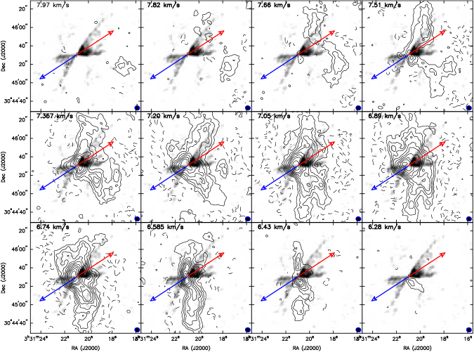
Figure 22: Channel maps of NH₃ (1,1) emission (contours) overlaid on CO ($J=1\rightarrow 0$) emission from Arce & Sargent (2006), showing the relationship between NH₃ emission and the outflow cavity. The top and bottom rows show the red- and blue-shifted component that are unblended; the NH₃ emission in the middle panels is blended. Contours start at $\pm$3$\sigma$, and then increase in 3$\sigma$ intervals. The negative contours are plotted as dashed lines, reflecting the loss of large-scale structure. The unblended velocity channels show very narrow structures and in the bottom row, the blue-shifted components are almost north-south in orientation. Much of the NH₃ emission south of the protostar appears unlikely to be influenced by the outflow. The position of the protostar is marked with the cross and the outflow axis is marked bye the blue and red lines denoting the outflow orientation within the plane of the sky.

Chen et al. (2007) suggested that the outflow may be interacting with the envelope, causing the gradient along the outflow. However, the IRAC data show that the outflow is well-collimated and appears only able to affect the material extended to the northwest of the protostar. To further examine the kinematic structure of this system, we have overlaid the NH₃ channel map contours on the CO map from Arce & Sargent (2006) in Figure 22. The top and bottom rows show the portions of the NH₃ lines that are not blended while in the middle panel the two lines are blended. At red-shifted velocities in the top panel, notice how the different parts of the emission come into view going toward lower velocities. The top right panel shows the red-shifted emission being emitted from two very thin structures running north-south. In the bottom panels of Figure 22, we can see that the more blue-shifted emission is still confined to a very thin structure running north-south; however, its location has shifted further to the east compared to the upper panels. Thus, we suggest that rather than an outflow interaction giving rise to the global velocity structure, a more probable explanation is that the envelope is filamentary and that the velocity shifts are flows along the filament toward the protostar. However, certain regions of the envelope that are spatially coincident with the outflow cavities may be affected by the outflow.

3.3.18 HH270 VLA1

HH270 VLA 1 is located in the L1617 cloud near Orion and is the driving source of the HH270 outflow (Reipurth et al., 1996; Rodríguez et al., 1998). This outflow in particular appears to be deflected and colliding with a neighboring core (the driving source of HH110 (Rodríguez et al., 1998)). In Paper I, we found that this protostar exhibits 8$\mu$m extinction in a filamentary envelope that is extended along the outflow and only on one side of the protostar. Furthermore, it was noted that the 4.5$\mu$m scattered light is brighter at the edge of the extincting envelope, indicating that extinction structure is indeed extended along the outflow and not due to a complex line of sight projection effect. The single-dish N₂H⁺ emission from this source is peaked on the 8$\mu$m extinction with no peak coincident with the protostar. The CARMA N₂H⁺ map is still tracing the 8$\mu$m extinction and shows a sharp decline of emission at the location of the protostar; the emission still appears one-sided even at high resolution.

The single-dish N₂H⁺ velocity map shows a gradient along the outflow with a linewidth enhancement just southwest of the protostar. This region of high linewidth is likely an unresolved velocity gradient, which is then resolved in the CARMA velocity map. The pattern in the CARMA velocity map closely matches the shape of the scattered light outflow cavity visible at 8$\mu$m in Figure 23. We suggest that these features are due to an outflow interaction with the surrounding material. We note that the data do not show a linewidth increase; therefore the outflow seems to be inducing bulk motion, but not an increase in linewidth.

4 Discussion

4.1 Large-Scale Velocity Field

The large-scale velocity gradients in dense molecular cores have long been interpreted as rotation (possibly solid-body) (e.g. Goodman et al., 1993; Caselli et al., 2002; Belloche et al., 2002; Belloche & André, 2004; Chen et al., 2007). If the large-scale motions are indeed rotation, then the circumstellar disk forming from the collapse of the surrounding envelope should be rotating in the same direction as the surrounding cloud, assuming axisymmetric collapse (e.g. Shu et al., 1987; Bodenheimer, 1995). However, if the core has fragmented, then the angular momenta of the individual disks could be misaligned, but the sum of the angular momenta would still be aligned with the cloud rotation. The direction of the jet and outflow of the system is commonly thought to reflect the current angular momentum vector of the protostar and disk system. This is because outflows and jets are thought to be related to the magnetic field of the protostar and disk which should be along the rotation axis (Pudritz & Norman, 1983; Shu et al., 1994) and resolved observations of disks have shown that jets are oriented normal to the disk midplane. Thus, we have used the outflow direction and protostar locations as guideposts as to where we should measure the velocity gradients relative to and in which direction because the equatorial plane of the envelope is where we are most likely to observe rotation.

The 2D fitting method (see Section 2.6.2) shows that eleven out of sixteen systems have a gradient direction that is within 45° of normal to the outflow axis in the single-dish data; however, there is considerable spread in this distribution. We caution that the PA of the gradients calculated by this method may have systematic error due to the velocity fields not being uniform and the velocities are sampled over a region that is not symmetric, leading to a bias of data points in a particular direction. Visual inspection of the velocity fields does yield a similar result to the 2D fitting, with eleven normal to the outflow and five not normal; IRAS 03282+3035, HH270 VLA1, L1527, L1521F, and L483 were not normal to the outflow. In contrast to the 2D fitting, we visually identify L483 and HH270 VLA1 as not normal to the outflow and L1157 and Serpens MMS3 to be normal. We further caution that most velocity fields have structure not easily described by a single position angle or velocity gradient. Nevertheless, as a simple significance test of the gradient-outflow direction relation, we can apply the binomial distribution if we consider the $<$45° and $\geq$45° as two bins and that the gradient direction relative to the outflow may be oriented randomly between 0 and 90° with a mean of 45° (Bevington, 1969). Thus, the probability of the relative directions falling within $<$45° or $>$45° should be equal. The chance of eleven or more objects out of sixteen with randomly oriented velocity gradients falling within the $\geq$45° bin is only $\sim$10%.

We also attempted to see if there is any trend with envelope mass and velocity gradient, we compared the observed velocity gradients and linewidths with the escape velocity in Figure 29. The envelope mass is calculated from the dust mass measured from 8$\mu$m extinction (Paper I, Table 1) plus 1 $M_{\sun}$ to account for the central object; note that the central object masses may be overestimated while the envelope masses are likely underestimated (Paper I). There is no apparent trend of velocity gradients or linewidth with increasing envelope mass (in terms of escape velocity). This figure further demonstrates that these protostellar systems are consistent with being gravitationally bound and are not supported by rotation or turbulence, consistent with many previous studies (e.g. Goodman et al., 1993; Caselli et al., 2002; Chen et al., 2007).

Furthermore, the smallest velocity gradients in our sample appear to be coming from the most symmetric envelopes L1521F, IRAS 16253-2429, and L1157, and the largest gradients are found in the morphologically complex HH211 and IRAS 03282+3035 systems. This could be taken to mean that the velocity structure is no strongly influenced by complex projection effects in the symmetric systems and are observing slow envelope rotation, while the more complex systems have projection effects altering the observed velocity structure. However, despite this trend, we note that the envelope of the low-luminosity source IRAM 04191 is approximately symmetric (Paper I) and has a velocity gradient of 17 km s^-1 pc^-1  (Belloche et al., 2002; Belloche & André, 2004), a clear counter-example to this morphological trend.

The simple interpretation of our velocity gradient data as a whole is that we are observing core rotation in these systems and that they have a variety of angular momenta ; some angular momenta being quite large (Figure 25). However, if we were observing pure rotation on large-scales, then one would expect the velocity gradient directions to be much more clustered toward being orthogonal to the outflow rather than the broad distribution shown in Figure 27. Therefore, either the complex morphology makes the rotation ambiguous, causing the velocity gradients to not be orthogonal to the outflow or we are not observing pure rotation. In either case, the angular momenta derived from the velocity gradients will be suspect at best. Given these complicating factors, we regard the velocity gradients taken as 1D cuts normal to the outflow as most likely to be probing the velocity gradients due to rotation, but these values should be regarded as upper limits.

If we are not observing pure rotation, the only other dynamical process which should give rise to ordered velocity structures are infall and/or outflow entrainment. The outflows from the protostars in our sample are highly collimated, limiting their ability to affect the large-scale kinematic structure, see Section 4.3 for further discussion, which leaves infall as the only other mechanism to contribute to the velocity field. This would require that infall is happening on large-scales and that collapse would need to be outside-in and not inside-out. Large-scale infall is shown to be possible in numerical simulations of complex, filamentary cores forming within a molecular cloud by Smith et al. (2011). Their simulations show that there is infall onto filaments (scales of 0.1 pc to 0.01 pc) from the surrounding molecular cloud, with subsequent infall from the filament to the protostar (sink particle) ($<$ 0.01 pc). Thus, infall convolved with rotation in real envelopes could lead to some of the complex velocity structures that we observe.

In summary, it is difficult to interpret the large-scale velocity gradients wholly being due to rotation since the envelopes are asymmetric and the gradients are often not normal to the outflow. Furthermore, flows or infall along a filament could give a similar signature to rotation simply from geometric projection, and if an envelope is filamentary, infall along the envelope would also produce a velocity gradient normal to the outflow. We therefore suggest that a component of infall velocity could be projected along our line of sight, entangled with the rotation velocity, resulting in the large velocity gradients. This issue of rotation versus projected infall will be further explored in an upcoming paper.

4.2 Small-scale Velocity Structure

The high-resolution interferometer data are essential for probing the kinematics of the envelope at scales smaller than 5000 AU. These data enable us to localize the gas in the envelope and to assess the dynamical processes at work. Small-scale velocity sub-structure, beyond an ordered/linear velocity gradient, is found in the interferometric observations of most envelopes, including L1157, L1165, HH108IRS, Serpens MMS3, L1527, CB230, IRAS 03282+3035, and RNO43. These features are sometimes apparent in the velocity maps or profiles shown in Figure 24, but they also appear as increased linewidth in the inner envelope. The small-scale velocity structure is generally found on $\sim$2000 AU scales in the envelopes. This radius could possibly be the centrifugal radius where material can be rotationally supported against gravity and the increased rotation velocity makes this region stand out against the rest of the envelope in velocity. However, assuming the large-scale velocity gradients reflect rotation, there would not be enough angular momentum for material to be rotationally supported at this radius.

We found that the relationship between outflow axis and velocity gradient direction in the interferometer data trends even more strongly toward being normal to the outflow that in the single-dish data. Twelve of fourteen systems have gradients within 45° of the outflow in the right panel Figure 27, as found by the 2D fitting technique. Using the same statistical analysis as the single-dish gradients, this result being due to chance is $\sim$0.6%. Note that this plot is missing L1157 and Serpens MMS3 since their complex velocity fields could not be reliably fit. Visually, we find that twelve envelopes clearly have gradients normal to the outflow and four do not (HH108MMS, L483, IRAS03282, and HH270VLA1); L483 and HH270 VLA1 were counted as within 45° of normal to the outflow. Note that RNO43, Perseus 5, and L1521F appear to have gradients normal to the outflow, but they also have complex velocity fields. L1157 is left out of this analysis because the gradient directions from the CARMA and VLA data differ by $\sim$80°.

The velocity gradient direction is generally consistent between both large and small scales in the single-dish and interferometer data as shown in Figure 28. This could mean that the dynamical processes observed at large-scales are also responsible for the kinematics observed at small-scales. The protostellar systems which show substantial deviation from large to small-scales are L1527 and L1521F. The difference in L1527 marks a velocity gradient reversal from large to small-scale (as also shown in Figure 24) and the difference in L1521F reflects that the kinematic structure was not well-resolved in the single-dish data. The N₂H⁺ and NH₃ lines in L1521F are also extremely optically thick making the velocity field derived from fitting uncertain since we cannot probe all the gas along the line of sight.

The preference for the vast majority of velocity gradients to be within 45° of normal to the outflow contrasts with Chen et al. (2007), where only two of nine targets had this feature. Moreover, in Volgenau et al. (2006), only one protostellar core of three observed had a well-ordered velocity structure. This result may be due to environment since the ordered structure was found in L1448 IRS3, a more isolated system, and the other sources were located in the more complex environment of NGC1333. Our sources in contrast are generally isolated, like those in Chen et al. (2007). As noted in the preceding paragraphs, we do see several objects with similarly complex velocity fields in our data; however, our greater number of observed systems likely enabled us to find more with ordered velocity fields.

The velocity gradients fit for the interferometer data are systematically larger than those found for the single-dish data, with the average being 8.6 km s^-1 pc^-1  from 1D fitting, the distribution is shown in Figure 26. This factor is nearly equal to our increase in resolution in the interferometer data as compared to the IRAM 30m, but the object-to-object increase is more varied. Some of the small-scale velocity structure is due to outflow interactions in the inner envelope as we will discuss in more detail in the following section; however, we have attempted to mask out these regions when fitting the velocity gradients. Like the single-dish data, we regard the 1D fitting method to more accurately reflect the velocity gradient intrinsic to the envelope itself since the 2D method will be more susceptible to outflow effects on the envelope kinematics. The only objects not showing large increase in the velocity gradient on small-scales are HH211 and IRAS 16253-2429 whose small-scale velocity gradient may be slightly overestimated.

We strongly cautioned in the previous section about interpreting the velocity gradients as rotation on large-scales and we are again hesitant to interpret the small-scale gradients as rotation and/or spin-up. This is because most envelopes are highly filamentary and on small-scales projections effects on the velocity structure will be even more apparent since both infall and rotation velocities increase at small radii. The velocity fields themselves on small-scales are not well-ordered as one might expect from rotationally dominated motion. Highlighting a few examples from Section 3.2: Serpens MMS3 shows deep red-shifted emission and increased linewidth only on one side of the protostar, the velocity gradient in HH108IRS reverses itself just past the protostar, the gradient in L1527 on small-scales is opposite of large scales, and RNO43 has an abrupt velocity jump across the envelope. The complex nature in the velocity fields of many sources do not necessitate an interpretation as rotation. Furthermore, infall velocities will always be necessarily be larger than rotation since the envelopes are not rotationally supported (Chen et al., 2007). Thus, the only way to robustly separate infall velocities from rotation is at $<$ 1000 AU scales, near the centrifugal radius where material can be rotationally supported.

Two systems in our sample (L1165 and RNO43) show high-velocity line wings in the inner envelope that could indeed reflect significant rotation. In both sources, the emission appears to be coming from a radius of $\sim$600 AU. Our data indicate that the observed velocities could reflect rotationally supported motion around $\sim$0.5$M_{\sun}$ central objects. Higher resolution and higher signal-to-noise data are needed to accurately centroid the high velocity emission in order to more precisely constrain the enclosed masses. In the future, ALMA could be used to spatially resolve the high-velocity emission in order to fully separate rotation from infall. Further analysis and modeling of the velocity structures observed with the interferometric data with the goal of determining the kinematic processes at work in the envelopes will be presented in an upcoming paper (Tobin et al. 2011 in preparation).

4.3 Outflow Induced Kinematic Structure

Our knowledge of protostellar outflows has been greatly enhanced in recent years (e.g. Bachiller, 1996; Arce et al., 2007, and references therein) and their possible effects on the surrounding envelope have been characterized (Arce & Sargent, 2006). Furthermore, IRAC imaging from the Spitzer Space Telescope, in addition to near-IR imaging from the ground, can give a strong constraint on the outflow axis and cavity width (e.g. Seale & Looney, 2008). These data complement observations of outflow tracers such as CO and give a more complete picture of how the outflow may be impacting the protostellar envelope.

Several protostars in the sample have velocity structures that are strongly suggestive of outflow effects on the N₂H⁺ and NH₃ gas kinematics. L1157, HH108MMS, and Perseus 5 appear to be significantly affected by the outflow, while HH108IRS, HH211, IRAS 03282+3035, L1152, and IRAS 04325+2402 only appear to be mildly affected. In the mildly affected cases, the large-scale bulk motion of the envelopes (line-center velocity) does not appear to be affected by the outflow, rather we see the effects in the linewidth at both large-scales and small-scales. This probably means that only a small portion of the total cloud mass is being affected by the outflow. The bulk motion effects are revealed in the strongly affected cases, generally on small-scales and only visible in the interferometer data.

Arce & Sargent (2006) presented an empirical model for how the outflow will affect the envelope during protostellar evolution, concluding that the outflow is ultimately responsible for disrupting the protostellar envelopes. The number of objects we find showing outflow effects in the kinematic data strongly support the outflow-envelope interaction framework put forward by Arce & Sargent (2006) and enable us to offer some further input to this empirical framework.

Perseus 5 and HH108MMS appear to be some of the youngest objects in our sample, as evidenced by their deeply embedded nature and lack of visible outflow cavities in 3.6$\mu$m or Ks-band imaging. In these systems, the outflow seems to be having the greatest impact on the kinematics in both line-center velocity and linewidth. Therefore, the effects of the outflow on the kinematic structure may be most prominent during its initial breakout of the envelope, early in the Class 0 phase. Smaller-scale effects on the envelope can clearly be seen in the case of L1157 where the envelope material may be entrained at 1000 AU scales. Thus, the outflows could be carrying significant momentum at wide angles near the protostar in order to be actively forcing inner envelope material out. If the outflows are impacting the envelope at small-scales and wide angles, an important question remains as to how much the outflow can quench infall in filamentary envelopes. In L1157, the amount of entrained gas appears tenuous, only $\sim$0.04 $M_{\sun}$ out of 0.7 $M_{\sun}$ in the inner envelope, following a simple analysis (Goldsmith & Langer, 1999) assuming an N₂H⁺ abundance of 10^-9 per H₂. On larger-scales ($>$ 1000AU), we expect that material extended normal to the outflow in filamentary envelopes will not be strongly influenced by the outflow, as the outflows appear to stay well collimated throughout the Class 0 phase.

4.4 Linewidths

The linewidths in the envelopes are generally quite small away from the protostar. In most cases, the linewidths are 0.2 - 0.5 km s^-1 in the single-dish data; linewidths averaged over the entire source are given Table 3. Note that these linewidths are substantially broader than the 10K thermal linewidth of N₂H⁺ which is $\sim$0.13 km/s, and is generally attributed to turbulent motions and/or unresolved velocity gradients along the line of sight. However, these linewidths are not large enough to make the envelope unbounded, as shown Figure 29.

The interferometer data find even smaller linewidths toward the outer edges of the envelopes; there were several cases where the lines are less than 2 channels wide. The narrow line-widths in the interferometer data likely stem from the larger scale structure being resolved out; the larger scale emission may have some turbulent or large-scale infall velocity component. The regions of broad linewidth in the interferometer observations appear to be directly related to the outflow, increased line-of-sight motion, and/or heating from the protostar; not a transition to a turbulent core (cf. Chen et al., 2007).

NH₃ linewidths were used by Pineda et al. (2010) to probe the kinematics of the large-scale molecular core, detecting a transition from the quiescent core to the turbulent cloud. We looked for such an effect in our sensitive N₂H⁺ data but did not find similar structure. We also did not detect N₂H⁺ emission on the scales for which Pineda et al. (2010) were able to detect NH₃, despite our high sensitivity. We believe that this is likely due to the differing critical densities between N₂H⁺ and NH₃ ($\sim$2$\times$10³ cm^-3 for NH₃ (1,1) and $\sim$1.4$\times$10⁵ cm^-3 for N₂H⁺ ($J=1\rightarrow 0$)).

We did, however, find that some maps (i.e. L673, HH211, HH108, RNO43) had regions with two distinct velocity components. The regions of overlap between the components appear as artificially large linewidths in the maps generated by the hyperfine fitting routine (section 2.6.1). We show three N₂H⁺ spectra from HH211 taken at three positions showing the different velocity components in Figure 30; this is indicative of what takes place in the other regions showing this feature. Notably, the additional velocity components tend to appear toward the edge of the maps, except in RNO43 where the transition takes place near the protostar. The distinct velocity components are located in regions that appear form a contiguous structure when viewed in 8$\mu$m extinction. The second velocity component generally appears about $\sim$0.05 pc from the nearest protostar. Thus, the reason for multiple components could have to do with the initial conditions of the clouds themselves. Recent simulations have suggested that colliding clouds could be an important component to setting up the initial conditions for star formation (e.g. Heitsch et al., 2006).

4.5 Chemical Effects on Molecular Tracers

The kinematic data presented are based on the molecular tracers N₂H⁺, NH₃, and HCO⁺. We have used N₂H⁺ and NH₃ relatively interchangeably, since they appear to trace the same kinematics and physical conditions (see Section 3.1 and Johnstone et al. (2010)). This makes sense because we know that in the pre-stellar phase, the formation of N₂H⁺ and NH₃ appear to be linked given their similar abundance distributions and only deplete onto dust grains at very high densities (Bergin & Tafalla, 2007). In many of our observations, N₂H⁺ and NH₃ only appear to trace the gas on scales $>$1000 AU from the protostar; the emission generally peaks near the protostar, but not directly on it. This indicates a drop in abundance either due to depletion or destruction of the molecules. Several of the protostars for which there are both interferometric NH₃ and N₂H⁺ observations (in this paper or in the literature) show decreased emission at the location of the protostar in both N₂H⁺ and NH₃. Observations of CB230 and IRAS 03282+3035 in NH₃ (Figures 6 and 21) and N₂H⁺ (Chen et al., 2007) are clear examples of NH₃ and N₂H⁺ not being peaked coincident with the protostar. L1157 also exhibits this effect in N₂H⁺ from the PdBI observations and also does in NH₃ if the longer baselines are given more weight in the VLA map. Finally, the low-luminosity source IRAM 04191 shows a similar depletion pattern in both of these tracers (Belloche & André, 2004, J. Mangum, Private Communication).

We can understand the decrease in N₂H⁺ emission in terms of molecular destruction by reactions with other molecules. In the inner envelope, where the temperatures rise above 20K, the CO that has depleted onto the dust grains (Bergin et al., 2002) is released back into the gas phase. CO and N₂H⁺ rapidly react to form HCO⁺; this is the dominant destruction mechanism for N₂H⁺ (Aikawa et al., 2001; Lee et al., 2004). This is the same reason that N₂H⁺ is not seen in outflows and why the N₂H⁺ is often not centrally peaked on the protostars in our interferometric observations. NH₃  however, is not directly destroyed by CO, but rather HCO⁺ (Lee et al., 2004). HCO⁺ will readily form within the region of CO evaporation making it available to react with NH₃. Alternatively, NH₃ could also become depleted onto dust grains in an ice mantle, and if it is well-mixed with the water ice, then it would only be evaporated at temperatures $\geq$100K. NH₃ ice is frequently observed in the envelopes surrounding protostars (Bottinelli et al., 2010) via mid-infrared spectroscopy. The absorbing NH₃ ice should be in the inner envelope since NH₃ only depletes onto grains at high densities. If any of the NH₃ ice were released into the gas phase, then HCO⁺ would be present to destroy it.

Since both NH₃ and N₂H⁺ are not present on scales $<$1000 AU, we must look for other tracers to probe the kinematic structure on these scales. In two protostars, we have been able to use HCO⁺ to trace the small-scale kinematic structure. The HCO⁺ emission from L1165 and RNO43 show high-velocity wings on small-scales inside the innermost N₂H⁺ emission; the centroids of the red and blue-shifted emission are offset from the protostar, normal to the outflow direction, at radii of $\sim$600AU.

Chemical models of an infalling protostellar envelope have been calculated by Lee et al. (2004), showing that HCO⁺ becomes enhanced at small-scales after formation of the protostar. This reflects the evaporation of CO ice, releasing CO back into the gas phase where HCO⁺ is readily formed. In addition, the primary destruction pathway of N₂H⁺ from CO results in the formation of HCO⁺ and N₂. Thus, we can see why the N₂H⁺ is tracing the gas at larger radii and lower velocities, while in the inner envelope HCO⁺ is readily being formed and can then trace the small-scale high-velocity gas.

Our dataset explicitly shows how multiple tracers can be used to gain a more complete picture of the kinematics in protostellar envelopes. N₂H⁺ and NH₃ are excellent tracers of the cold, dense gas on scales from $\sim$1000-2000 AU out to $\sim$10000-20000 AU. Inside of 1000AU, an abundant tracer of the warm, inner envelope tracer must be observed; HCO⁺ works quite well in two out of nine sources observed with CARMA and other tracers and/or higher-J transitions of HCO⁺ may work as well (see Lee et al. (2009) and Brinch et al. (2007)). However, these other tracers are often found in outflows and they must be observed with sufficiently high resolution to confirm their origin in the envelope and not the outflow. In the future, ALMA may be able to observe inner envelope tracers to resolve the motion of the dense gas in the inner envelope, tracing infall onto the disk.

5 Summary

We have conducted a single-dish and interferometric survey mapping emission of the dense gas tracers N₂H⁺ ($J=1\rightarrow 0$) and/or NH₃ (1,1) in envelopes around low-mass protostars. Many of these envelopes are known to be morphologically complex from 8$\mu$m extinction mapping. We used these data to map the line-center velocity and linewidth across these envelopes. We quantitatively measured the velocity gradients and their directions in order to characterize the dense gas kinematics in the complex protostellar envelopes, our specific results are as follows.

1. Ordered velocity fields are present on large-scales in most protostellar envelopes from the single-dish sample. In eleven out of sixteen cases, the velocity gradients appear to be within 45° of normal to the outflow axis with an average gradient of $\sim$ 2.3 km s^-1 pc^-1 , depending on fitting method. The velocity gradients could be due to core rotation; however, the velocity gradient position angles do have a broad distribution with respect to the outflow direction. Furthermore, the strongly asymmetric nature of the envelopes and the fact that most envelopes in the sample are substantially bound leads us to suggest that we may be seeing a component of infall projected along our line of sight entangled with rotation. We find evidence of multiple components of N₂H⁺ emission in several clouds, possibly relating our observations to a colliding-cloud formation scenario.

2. The small-scale kinematic structure observed by the interferometers appears to be gravitationally dominated by the central protostar and it likely originates from a combination of infall and rotation in some cases. The average velocity gradient in the interferometer data is 8.6 km s^-1 pc^-1 , with gradient directions within 45^° of normal to the outflow in twelve out of fourteen cases. The complex velocity fields in many systems suggest that interpreting the velocity gradients as pure rotation is incorrect. Only on the smallest scales ($<$1000 AU) will rotation differentiate itself from infall. Furthermore, multiple tracers must be used to gain a complete picture of the kinematic structure of the envelope down to sub-1000 AU scales due to depletion of the cold gas tracers within $\sim$1000 AU. In the cases of RNO43 and L1165, we were able to use HCO⁺ $(J=1\rightarrow 0)$ to trace inner envelope kinematics on scales of $\sim$600 AU.

3. Outflows do impact the envelope kinematics derived from NH₃ and N₂H⁺ in some systems and their effects are most prominent at $\sim$1000-2000 AU scales. Clear outflow effects on the large-scale kinematics in the single-dish data are only seen for five systems, but the only evident kinematic effect is increased linewidth along the outflow. The effects are most pronounced in the interferometer data for the deeply embedded sources HH108MMS and Perseus 5. Furthermore, we see a remarkable case of the outflow possibly entraining the inner envelope of L1157 on $\sim$1000 AU scales.

The authors thank the anonymous referee for a thorough report which improved the paper as a whole and H. Arce for providing the OVRO CO data of IRAS 03282+3035. We would also like to thank A. Goodman, S. Offner, Y. Shirley, A. Stutz, W. Kwon, J. Lee, and P. Myers for useful discussions. We wish to thank the CARMA observers for carrying out the observations. We thank V. Piétu for assistance with the PdBI data reduction and C. Buchbender for assistance in conducting observations at the 30m in addition to the IRAM staff as a whole. Support for CARMA construction was derived from the states of Illinois, California, and Maryland, the James S. McDonnell Foundation, the Gordon and Betty Moore Foundation, the Kenneth T. and Eileen L. Norris Foundation, the University of Chicago, the Associates of the California Institute of Technology, and the National Science Foundation. Ongoing CARMA development and operations are supported by the National Science Foundation under a cooperative agreement, and by the CARMA partner universities. The National Radio Astronomy Observatory is a facility of the National Science Foundation operated under cooperative agreement by Associated Universities, Inc. IRAM is supported by INSU/CNRS (France), MPG (Germany) and IGN (Spain). J. J. Tobin acknowledges support from HST-GO-11548.04-A, the University of Michigan Rackham Dissertation Fellowship, and Spitzer archival research program 50668.

Facilities: IRAM:30m, CARMA, VLA, IRAM:Interferometer, Spitzer (IRAC), Blanco (ISPI)

Appendix A Continuum Data

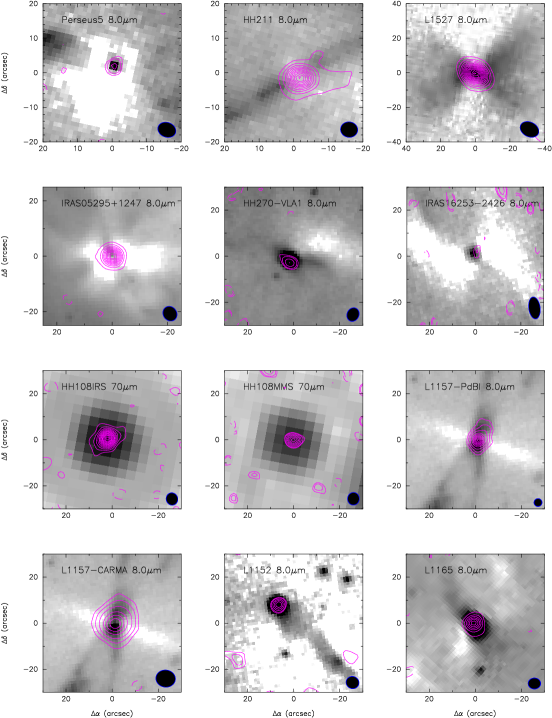
Figure 31: IRAC 8$\mu$m images of sources observed, with CARMA $\lambda$=3mm continuum contours overlaid. For most protostars, the continuum emission is directly coincident with the 8$\mu$m point sources; 70$\mu$m in the case of HH108IRS/MMS. The contours for Perseus 5, HH270, IRAS 16253-2429, HH108MMS, and L1152 are $\pm$2.5$\sigma$, 3,4,5,…,9$\sigma$ and then increase in 3$\sigma$ intervals. The contours for HH211, L1527, RNO43, HH108IRS, and L1165 start at $\pm$3$\sigma$ and increase by 3$\sigma$. The contours for L1157 are $\pm$3, 6, 12, 24, 36, 48, 60, 72, 84, and 96$\sigma$.

In conjunction with our CARMA and PdBI N₂H⁺ observations, the 3mm continuum emission was observed for those 11 sources. The continuum data are overlaid on the IRAC 8$\mu$m images for all but HH108IRS/MMS (we shown 70$\mu$m data due to lack of IRAC imaging) in Figure 31. The 3mm continuum sources are point-like in most cases, HH108IRS and HH211 appear to show extended structure at the 3$\sigma$ level, consistent with envelope dust emission. L1157, L1165, and HH270 are also slightly extended, but in the direction of their outflows, indicating that there may be a component of free-free jet emission or heated dust along the outflow in the 3mm continuum data. In all cases, the continuum sources are coincident with the 8$\mu$m/70$\mu$m point sources. There are a few cases (L1157, HH211, and RNO43) where there is not a clear point source at 8$\mu$m and the 3mm emission is located between the outflow cavities where there is significant extinction. In these cases, the 24$\mu$m point source is then found to peak at the same location of the 3mm source. We note that the protostar IRAS 16253-2429 shows a slight offset between the 8$\mu$m point source and the continuum detection; however, the detection is barely 3$\sigma$, thus we do not believe that this offset is real. The continuum fluxes at 3mm are listed in Table 11.

Figure 5: L1165– The left panel shows the IRAC 8$\mu$m image with CARMA HCO⁺ blue and red-shifted emission, summed over -3.5 to -2 km s^-1 and -1.0 to 0 km s^-1, plotted as blue and red contours respectively. The contours levels are $\pm$3, 6, and 8.25$\sigma$ ($\sigma$=0.175 K) for the blue-shifted emission and $\pm$3, 9, 18, and 27$\sigma$ ($\sigma$=0.212 K) for the red-shifted emission. The blue and red-shifted emission from HCO⁺ is located symmetrically about the protostar, normal to the outflow. The dashed lines mark the regions where the position-velocity cut was taken and point to respective ends of the PV plot in the right panel. The position of the protostar/continuum source is marked with a white cross. The position-velocity cut shows that the blue and red-shifted emission traces higher velocity material and there is a slight gradient of material going to higher velocity closer to the continuum source. The PV plot contours start at 3$\sigma$ and increase in 3$\sigma$ intervals ($\sigma$=0.2). The solid-blue curve represents Keplerian rotation (or infall) for a 0.5 $M_{\sun}$ central object and the dashed-blue curve is for a 2.0 $M_{\sun}$ central object.

Figure 24: Line center velocity cuts taken across each protostellar envelope, normal to the outflow. The diamonds are the single-dish data and the plus-signs are the interferometer data. Each point for the single-dish data is the average of the 27^′′ beam surrounding each point. Each interferometer point is the average of points within the semi-major axis of the synthesized beam. The velocity errors at each point are generally $<$0.05 km s^-1, approximately the size of the symbols. The solid-lines are the linear fits to the single-dish velocity data between $\pm$30″ for most sources. Serpens MMS3 was fit between 60″ and 0″ and L1152 was fit between 40″ and -20″.

Fig. 24 — cont’d.

Fig. 24 — cont’d.

Figure 25: Histogram plots of measured velocity gradients from single-dish data. The left panel shows the velocity gradients derived from one-dimensional cuts across the velocity field, taken normal to the outflow. The middle panel shows the velocity gradients derived from a two-dimensional fit to the velocity field. The right panel shows the velocity gradients derived from the velocity difference at $\pm$10000 AU from the protostar, also normal to the outflow. The distributions from the one- and two-dimensional fits are comparable while the two point method is skewed toward smaller gradients; this difference is likely due to the gradients fits picking up on higher velocity emission that sometimes turns over toward lower velocities by $\sim$ 10000 AU. The middle panel include the two-dimensional fit for L673 which is absent from the left and right panels.

Figure 26: Histogram plots of measured velocity gradients from interferometer data. The left panel shows the velocity gradients derived from one-dimensional cuts across the velocity field, taken normal to the outflow. The right panel shows the velocity gradients derived from a two-dimensional fit to the velocity field. The differences in these distributions likely result from the two-dimensional method having to fit all the data where complexities in the velocity field may reduce the gradient fit. The left panels include L1157 and Serpens MMS3 while they are absent from the right panels.

Figure 27: Histogram plots of velocity gradient position angle offset relative to outflow position angle for single-dish (left panel) and interferometric (right panel) velocity gradient measurements. An offset of 90^∘ indicates that the gradient is normal to the outflow and most of the velocity gradients are within 45^∘ of normal to the outflow (dashed line); however, there is substantial dispersion in this relationship. The shift in number toward 90° in the interferometer observations may reflect that smaller-scale motion is becoming more ordered. The left panels include L1157 and Serpens MMS3 while they are absent from the right panels.

Figure 28: Histogram plot of single-dish velocity gradient position angle minus the interferometric velocity gradient position angle. Most velocity gradients at large and small-scales are within 45° of each other, indicating that the line of sight velocities at large-scales reflect similar velocity structure at small-scales. This plot does not include L1157, Serpens MMS3, or L673.

Figure 29: Plot of escape velocity at 10000 AU versus velocity shifts measured at 10000 AU radii (diamonds) and the average N₂H⁺ FWHM from the single-dish data (squares). The escape velocity is calculated using the total mass of the envelope from the 8$\mu$m extinction data in Paper I plus a 1 $M_{\sun}$ solar mass central object; the error bars in the calculated escape velocity reflect a 50% uncertainty in total mass. This shows that the envelopes are consistent with being gravitationally bound on large-scales and that the envelopes are not supported by rotation, turbulence, and/or thermal pressure. The protostar closest to rotational support is HH211; its substantial rotation was also highlighted by Tanner & Arce (2011).

Figure 30: Plot of single-dish N₂H⁺ line profiles at three positions in HH211 showing the transition between different velocity components. The middle spectrum is in the region where the two components are blended, demonstrating that the lines are not extremely wide.

Table 1: Source Properties

Source	RA	Dec	Distance	Mass8μm	Masssubmm	Lbol	Tbol	Morphological	Outflow PA	References
	(J2000)	(J2000)	(pc)	($M_{\sun}$)	($M_{\sun}$)	($L_{\sun}$)	(K)	Classification	(°)	(Distance, Mref, Lbol,)
				(r$<$0.05pc)						(Tbol, Outflow PA)
Perseus 5	03:29:51.88	+31:39:05.7	230	2.0	1.24	0.46	41	One-sided	80	23, 17, 3, 3, 1
IRAS 03282+3035	03:31:21.10	+30:45:30.2	230	2.4	2.2	1.2	33	Irregular	122	23, 4, 3, 3, 26
HH211	03:43:56.78	+32:00:49.8	230	1.1	1.5	3.02	24	Irregular	116	23, 3, 3, 3, 6
L1521F	04:28:39.03	+26:51:35.0	140	2.3	1.0	0.03	$\sim$20	Spheroidal	270	20, 10, 8, 1, 7
IRAS 04325+2402	04:35:35.39	+24:08:19.0	140	-	-	0.97	73	Binary Core	200	20, -, 15, 15, 16
L1527	04:39:53.86	+26:03:09.5	140	0.8	2.4	0.9	56	One-sided	90	20, 4, 9, 15, 31
RNO43	05:32:19.39	+12:49:40.8	460	2.8	2.6	12.5	56	Irregular	20	21, 10, 2, 15, 21 & 1
HH270 VLA1	05:51:34.64	+02:56:45.8	420	1.9	-	7.0	32	One-sided	240	22, -, 2, 1, 1
IRAS 16253-2429	16:28:21.42	-24:36:22.1	125	0.8	0.98	0.25	35	Spheroidal	20	19, 10, 3, 3, 26
L483	18:17:29.93	-04:39:39.6	200	3.5	1.8	11.5	$<$54	Irregular	282	25, 4, 3, 15, 30
Serpens MMS3	18:29:09.13	+00:31:31.6	400	0.95	2.2	1.6	39	Flattened	180	18, 3, 14, 3, 1
HH108IRS	18:35:42.14	-00:33:18.5	300	-	4.5	$\sim$8.0	28	Flattened	208	17, 14, 14, 1, 1
HH108MMS	18:35:46.46	-00:32:51.2	300	-	3.6	0.7	18	Flattened	130	17, 17, 1, 1, 1
L673-SMM2	19:20:25.96	+11:19:52.9	300	1.0	0.35	2.8	-	Flattened	270, 135	24, -, -, 12, 1 & 12
L1152	20:35:46.22	+67:53:01.9	300	3.4	12.0	1.0	33	Binary Core	225	5, 10, 3, 1, 13
L1157	20:39:06.25	+68:02:15.9	300	0.86	2.2	3.0	29	Flattened	150	5, 4, 3, 15, 27
CB230	21:17:38.56	+68:17:33.3	300	1.1	1.1	7.2	69	One-sided	0	5, 11, 3, 15, 28
L1165	22:06:50.46	+59:02:45.9	300	1.1	0.32	13.9	46	Irregular	225	5, 1, 12, 1, 12

Note. — Properties of sources observed in the single-dish and/or interferometric sample. The 8$\mu$m extinction masses are taken within 0.05 pc of the protostar and note that some of the masses have been rescaled to account for a different distance estimate as compared to Paper I. Positions are reflect the coordinates of the 24$\mu$m point source from Spitzer data or the 3mm continuum continuum position for protostars observed with CARMA. The Outflow position axes (PA) are not well constrained since the outflows are known to precess they can have fairly large angular width; a conservative estimate of uncertainty would be $\pm$10°. References: (1) This work, (2) Tobin et al. (2010b), (3) Enoch et al. (2009), (4) Shirley et al. (2000), (5) Kirk et al. (2009), (6) Lee et al. (2009), (7) Bourke et al. (2006) (8) Terebey et al. (2009), (9) Tobin et al. (2008), (10) Young et al. (2006), (11) Kauffmann et al. (2008) (12) Visser et al. (2002), (13) Chapman & Mundy (2009), (14) Enoch et al. (2007), (15) Froebrich (2005), (16) Hartmann et al. (1999), (17) Chini et al. (2001), (18) Dzib et al. (2010), (19) Loinard et al. (2008), (20) Loinard et al. (2007), (21) Bence et al. (1996), (22) Menten et al. (2007), (23) Hirota et al. (2011), (24) Herbig & Jones (1983), (25) Jørgensen (2004), (26) Arce & Sargent (2006), (27) Gueth et al. (1996), (28) Launhardt et al. (2001), (29) Stanke et al. (2006), (30) Fuller et al. (1995), (31) Hogerheijde et al. (1998).

Table 2: IRAM 30m Observations

Source	RA	Dec	Receiver	Date	$\sigma_{T}$	$\Delta v$
	(J2000)	(J2000)		(UT)	(mK)	(km s-1)
IRAS 03282$+$3035	03:31:19.8	+30:45:37	EMIR E090	25 Oct 2009	60	0.067
HH211-mm	03:43:55.3	+32:00:46	EMIR E090	24 Oct 2009	70	0.067
L1521F	04:28:39.0	+26:51:37	EMIR E090	24 Oct 2009	200	0.067
IRAS04325+2402	04:35:36.6	+24:08:54	EMIR E090	25 Oct 2009	60	0.067
L1527	04:39:54.0	+26:03:22	EMIR E090	26 Oct 2009	50	0.067
RNO43	05:32:18.2	+12:50:01	EMIR E090	24 Oct 2009	50	0.067
HH270 VLA1	05:51:33.6	+02:56:46	AB100	27 Dec 2008	50	0.067
IRAS 16253-2429	16:28:21.9	-24:36:22	AB100	29 Dec 2008	170	0.067
L483	18:17:30.3	-04:39:40.6	EMIR E090	25 Oct 2009	75	0.067
Serpens MMS3	18:29:10.2	+00:31:18	EMIR E090	24 Oct 2009	200	0.067
HH108	18:35:42.7	-00:33:07	EMIR E090	23 Oct 2009	80	0.067
L673-SMM2	19:20:25.4	+11:19:44	EMIR E090	23/24 Oct 2009	65	0.067
L1152	20:35:47.17	+67:53:22	EMIR E090	24 Oct 2009	55	0.067
L1157	20:39:05.6	+68:02:13.2	EMIR E090	25 Oct 2009	30	0.067
CB230	21:17:28.7	+68:17:42.8	AB100	26 Dec 2008	50	0.067
L1165	22:06:50.8	+59:03:06.5	EMIR E090	25 Oct 2009	60	0.067

Note. — Observations of protostellar envelopes taken with the IRAM 30m telescope. The positions reflect the map center and not necessarily the protostar position.

Table 3: CARMA Observations

Source	RA	Dec	Config.	Date	Calibrators	Beam	$\sigma_{T}$	$\Delta v$
	(J2000)	(J2000)		(UT)	(Gain, Flux)	(″)	(mK)	(km s-1)
Perseus 5	03:29:51.84	+31:39:06.2	D-array	10 Apr 2010	0336+323, Uranus	5.2$\times$4.1	450	0.067
HH211-mm	03:43:56.8	+32:00:50.3	D-array	16 Apr 2010	0336+323, Uranus	5.0$\times$4.3	400	0.067
L1527	04:39:53.9	+26:03:09.6	E-array	02/05/06 Oct 2008	3C111, 3C84	11.1$\times$8.2	100	0.1
RNO43	05:32:19.1	+12:49:43.1	D-array	18/22 Apr 2010	0532+075, Mars	5.5$\times$4.6	300	0.067
..	..	..	..	2 Sept. 2010	0532+075, Uranus	..	..	0.067
HH270 VLA1	05:51:33.6	+02:56:47.2	D-array	24/25/26 Jul 2009	0532+075, Mars	5.9$\times$5.0	500	0.1
IRAS 16253-2429	16:28:21.6	-24:36:23.1	D-array	12 Aug 2009	1625-254, MWC349	9.3$\times$4.9	500	0.1
HH108 IRS	18:35:42.17	-00:33:18.3	D-array	10 Apr 2010	1830+063, Neptune	5.9$\times$5.0	500	0.067
HH108 MMS	18:35:46.53	-00:32:51.4	D-array	14/15 Apr 2010	1830+063, MWC349	5.9$\times$5.0	450	0.067
L1152	20:35:44.14	+67:52:51.3	D-array	11 Apr 2010	1927+739, MWC349	5.4$\times$5.1	600	0.067
L1157	20:39:06.3	+68:02:15.8	D-array	19/29 Mar 2009	1927+739, MWC349	7.3$\times$6.6	150	0.1
..	..	..	E-array	02 Oct 2008	1927+739, MWC349	..	..	0.1
L1165	22:06:50.32	+59:02:45.5	D-array	25 Jul 2009	2038+513, MWC349	5.3$\times$4.7	400	0.1

Note. — Observation parameters of protostars observed with CARMA, the coordinates listed for each protostar denote the phase center of the observation, not necessarily the position of the protostar. The frequency resolution for the 2010 observations was 0.067 km s^-1; however, this was rebinned to 0.1 km s^-1 to increase signal-to-noise. The observations of L1165, IRAS 16253-2429, and HH270 VLA 1 only observed the central three hyperfine N₂H⁺ lines, while the observation of L1157 and L1527 observed the isolated N₂H⁺ line. All other observations observed all 7 N₂H⁺ hyperfine transitions.

Table 4: Very Large Array Observations

Source	RA	Dec	Config.	Date	Calibrators	Beam	$\sigma_{T}$	$\Delta v$
	(J2000)	(J2000)		(UT)	(Gain, Flux)	(″)	(mK)	(km s-1)
IRAS 03282$+$3035	03:31:20.34	+30:45:32.0	D-array	12 Nov 2009	0336+323, 3C48	5.2$\times$4.6	240	0.15
L1521F	04:28:38.9	+26:51:35.0	D-array	19 Mar 2007	0418+380, 3C48	7.1$\times$6.7	125	0.075
L1527	04:39:53.9	+26:03:09.6	D-array	07 Mar 2003	0510+180, 3C48	4.8$\times$4.1	300	0.15
L483	18:17:29.83	-04:39:38.3	D-array	18 Apr 1995	1751+096, 3C286	6.3$\times$5.9	300	0.3
Serpens MMS3	18:29:09.1	+00:31:34.0	D-array	11/12 Nov 2009	1851+005, 3C48	5.6$\times$5.3	270	0.15
L673-SMM2	19:20:26.27	+11:20:08.2	D-array	6 Nov 2009	1925+211, 3C286	5.4$\times$5.0	250	0.15
L1157	20:39:06.3	+68:02:15.0	D-array	2/3 Jan 2010	1927+739, 3C48	4.6$\times$4.0	250	0.15
CB230	21:17:37.59	+68:17:38.5	D-array	18/20 Oct 2009	2022+616, 3C48	4.5$\times$3.3	325	0.15

Note. — Observation parameters of protostars observed with VLA, the coordinates listed for each protostar denote the phase center of the observation, not necessarily the position of the protostar. The frequency resolution of the L1521F observation was 0.075 km s^-1; however, this was rebinned to 0.15 km s^-1 to increase signal-to-noise.

Table 5: Plateau de Bure Interferometer Observations

Source	RA	Dec	Config.	Date	Calibrators	Beam	$\sigma_{T}$	$\Delta v$
	(J2000)	(J2000)		(UT)	(Gain, Flux)	(″)	(mK)	(km s-1)
L1157	20:39:05.6	+68:02:13.2	D-array	17 Jun, 07 Jul 2009	1927+739, MWC349	3.4$\times$3.3	80	0.125
..	..	..	C-array	13 Nov 2009	1927+739, MWC349	..	..	0.125

Note. — Observation parameters of the protostar observed with the PdBI, the coordinates listed denote the phase center of the observation, not necessarily the position of the protostar.

Table 6: Single-Dish N₂H⁺ Properties

Source	Vlsr	FWHM	I${}_{max}\pm\sigma_{I}$	$\tau_{tot}$	Tex	N(N2H+)	N2H+ Mass	Radius
	(km s-1)	(km s-1)	(K km s-1)		(K)	(cm-2)	(10-9 $M_{\sun}$/X(N2H+))	(″)
IRAS 03282+3035	7.1	0.67	5.9$\pm$0.04	4.9	6.4	1.8$\times$1013	1.4	160$\times$80
HH211-mm	9.1	0.5	5.8$\pm$0.05	6.9	5.2	2.3$\times$1013	1.4	120$\times$110
L1521F	6.45	0.29	4.0$\pm$0.14	17.5	4.7	4.1$\times$1013	1.9	160$\times$110
IRAS 04325+2402	5.9	0.45	5.4$\pm$0.04	5.4	6.8	1.9$\times$1013	2.4	180$\times$160
L1527	5.9	0.36	3.1$\pm$0.03	9.3	4.3	1.7$\times$1013	0.9	180$\times$160
RNO43	10.25	0.69	2.5$\pm$0.04	0.9	5.6	2.3$\times$1013	0.8	90$\times$80
HH270 VLA1	8.9	0.41	2.5$\pm$0.04	4.6	4.2	6.5$\times$1012	1.2	135$\times$65
IRAS 16253-2429	4.05	0.3	4.2$\pm$0.13	6.6	5.6	1.7$\times$1013	0.4	100$\times$80
L483	5.5	0.51	10.3$\pm$0.06	16.1	5.4	9.1$\times$1013	10.4	200$\times$150
Serpens MMS3-full	8.5	0.62	12.5$\pm$0.12	6.6	6.9	6.1$\times$1013	21.5	200$\times$150
Serpens MMS3-proto	8.5	0.62	5.4$\pm$0.12	3.5	6.1	1.5$\times$1013	1.9	no boundary
HH108-full	11.0	0.54	4.7$\pm$0.05	4.0	5.6	1.1$\times$1013	2.35	160$\times$50
HH108IRS	11.0	0.54	4.7$\pm$0.05	4.0	5.6	1.1$\times$1013	0.9	no boundary
HH108MMS	10.9	0.54	1.9$\pm$0.05	2.5	5.1	3.0$\times$1012	0.4	no boundary
L673-SMM2	7.1	0.48	7.1$\pm$0.04	2.6	8.5	1.6$\times$1013	5.3	$\sim$150$\times$80
L1152	2.5	0.47	5.4$\pm$0.04	7.3	5.5	2.4$\times$1013	3.9	260$\times$95
L1157	2.65	0.39	4.6$\pm$0.02	4.5	4.8	1.4$\times$1013	3.0	200$\times$70
CB230	2.8	0.5	4.0$\pm$0.04	3.6	5.0	8.9$\times$1012	1.0	115$\times$75
L1165	-1.50	0.42	2.5$\pm$0.04	5.6	4.2	8.3$\times$1012	0.6	90$\times$60

Note. — The N₂H⁺ properties of each source are tabulated, column densities are scaled by 1.17 to account for beam efficiency. The FWHM linewidth is taken from the average single-dish spectrum over the entire envelope. The statistical uncertainty in the linewidth is less than 0.01 km s^-1; however, this value varies across the envelope and will vary depending on the region averaged. The optical depth, T_ex, column density are measured at the N₂H⁺ emission peak; however, multiple positions are quoted for HH108 and Serpens MMS3. The envelope mass is computed by summing the column density over the entire emitting region and assuming a constant N₂H⁺ abundance of 1.0$\times$10^-9 relative to H₂. The envelope radius is measured where the N₂H⁺ is 10% of the peak. The optical depths, column densities, and masses should only be regarded as accurate within factors of a few owing to systematic errors in calculation of optical depth and excitation temperature.

Table 7: Interferometric N₂H⁺ Properties

Source	Vlsr	FWHM	I${}_{max}\pm\sigma_{I}$	$\tau_{tot}$	Tex	N(N2H+)	N2H+ Mass	Radius
	(km s-1)	(km s-1)	(K km s-1)		(K)	(cm-2)	(10-9 $M_{\sun}$/X(N2H+))	(″)
Perseus 5	8.06	0.29	6.1$\pm$0.28	3.1	13.1	3.0$\times$1013	0.3	20
HH211-mm	9.12	0.39	8.3$\pm$0.25	9.9	8.4	9.3$\times$1013	1.1	40
L1527	6.01	0.26	0.9$\pm$0.05	8.8	4.8	1.8$\times$1013	0.2	57
RNO43	9.87, 10.5	0.43, 0.32	3.0$\pm$0.19	5.5	6.7	1.8$\times$1013	0.4	23
HH270 VLA1	8.86	0.41	6.0$\pm$0.24	4.9	11.2	3.5$\times$1012	0.9	28
IRAS 16253-2429	4.12	0.21	4.4$\pm$0.24	7.4	7.6	3.2$\times$1013	1.5	36
HH108IRS	10.8	0.59	14.1$\pm$0.3	8.2	12.5	8.4$\times$1013	1.2	21
HH108MMS	10.9	0.40	5.0$\pm$0.3	8.4	6.4	4.3$\times$1013	0.7	12
L1152	2.63	0.34	9.6$\pm$0.36	10.1	10.7	1.3$\times$1014	4.3	29
L1157 (PdBI)	2.7	0.74	19.8$\pm$0.06	10.4	8.0	1.2$\times$1014	0.7	25
L1157 (CARMA)	2.7	1.0	16.7$\pm$0.06	4.8	8.5	4.7$\times$1013	0.8	41
L1165	-1.5	0.38	6.6$\pm$0.21	6.6	8.0	4.5$\times$1013	0.4	17

Note. — The N₂H⁺ properties of each source are tabulated. The V_lsr and FWHM linewidth are taken from the position of peak intensity. The statistical uncertainty in the linewidth is less than 0.01 km s^-1; however, the linewidth varies across the envelope. The optical depth, T_ex, column density are measured at the N₂H⁺ emission peak. The envelope mass is computed by summing the column density over the entire emitting region and assuming a; regions of bad data toward edges are masked out of the measurement. The optical depths, column densities, and masses should only be regarded as accurate within factors of a few owing to systematic errors in calculation of optical depth and excitation temperature.

Table 8: Interferometric NH₃ Properties

Source	Vlsr	FWHM	I${}_{max}\pm\sigma_{I}$	Optical Depth	Tex	N(NH3)	NH3 Mass	Radius
	(km s-1)	(km s-1)	(K km s-1)		(K)	(cm-2)	(10-8 $M_{\sun}$/X(NH3))	(″)
IRAS 03282+3035	6.98	0.38	6.4$\pm$0.13	10.1	12.7	1.4$\times$1015	5.7	60
L1521F	7.11	0.37	1.4$\pm$0.06	10.1	3.9	8.0$\times$1015	29.3	49
L1527	5.95	0.26	2.6$\pm$0.16	1.0	10.45	3.9$\times$1014	1.4	39
L483	5.41	0.51	5.8$\pm$0.18	6.8	8.3	2.3$\times$1015	27.7	62
Serpens MMS3	8.22	0.51	7.0$\pm$0.19	2.1	10.2	2.0$\times$1015	7.5	50
L673-SMM2	6.93	0.50	8.4$\pm$0.14	0.53	33.3	7.2$\times$1014	11.3	76
L1157	2.71	0.56	8.6$\pm$0.15	1.6	13.4	8.5$\times$1014	16.0	87
CB230	2.78	0.47	6.5$\pm$0.22	1.1	16.9	6.1$\times$1014	4.8	36

Note. — The NH₃ properties of each source are tabulated. The V_lsr and FWHM linewidth are taken from the position of peak intensity. The statistical uncertainty in the linewidth is less than 0.01 km s^-1; however, the linewidth varies across the envelope. The optical depth, T_ex, column density are measured at the NH₃ emission peak except. The envelope mass is computed by summing the column density over the entire emitting region and assuming a constant NH₃ abundance of 1.0$\times$10^-8 relative to H₂; regions of bad data toward edges are masked out of the measurement. The optical depths, column densities, and masses should only be regarded as accurate within factors of a few owing to systematic errors in calculation of optical depth and excitation temperature. The masses from NH₃ also appear to be overestimating the actual envelope masses, compared to the 8$\mu$m and submillimeter dust masses; thus, the NH₃ abundance relative to H₂ could be larger than assumed.

Table 9: Single-Dish Velocity Gradients

Source	Gradient	Gradient Fit	Gradient Fit	Gradient PA	Gradient PA
	(10000AU)	1D	2D	2D	- Outflow PA
	(km s-1 pc-1)	(km s-1 pc-1)	(km s-1 pc-1)	(∘)	(∘)
Perseus 5	-	-	-	-	-
IRAS 03282+3035	1.13$\pm$0.2	1.31 $\pm$0.004	4.6$\pm$0.04	301$\pm$0.5	1
HH211-mm	7.2$\pm$0.3	6.9$\pm$0.03	4.2$\pm$0.07	31$\pm$0.9	85
L1521F	0.26$\pm$0.13	0.13$\pm$0.002	0.76$\pm$0.02	239$\pm$1.8	31
IRAS 04325+2402	3.1$\pm$0.11	5.2$\pm$0.01	3.5$\pm$0.01	79$\pm$0.3	59
L1527	2.7$\pm$0.29	2.2$\pm$0.01	2.2$\pm$0.02	114$\pm$0.5	24
RNO43	2.5$\pm$0.9	2.2$\pm$0.1	3.3$\pm$0.4	280$\pm$4.6	80
HH270 VLA1	0.98$\pm$0.2	0.88$\pm$0.004	1.4$\pm$0.04	166$\pm$1.3	74
IRAS 16253-2429	0.8$\pm$0.18	1.2$\pm$0.002	1.7$\pm$0.04	311$\pm$1.3	69
L483	3.7$\pm$0.24	3.6$\pm$0.01	2.2$\pm$0.02	66$\pm$0.4	36
Serpens MMS3	1.5$\pm$0.24	1.4$\pm$0.01	1.1$\pm$0.01	307$\pm$0.6	53
HH108IRS	0.64$\pm$0.24	2.0$\pm$0.004	1.2$\pm$0.03	96$\pm$2.1	68
HH108MMS	1.7$\pm$0.13	1.6$\pm$0.004	2.0$\pm$0.05	67$\pm$1.6	62
L673-SMM2	-	-	1.0$\pm$0.02	100$\pm$2.1	10
L1152	1.7$\pm$0.42	2.7$\pm$0.004	3.2$\pm$0.04	145$\pm$0.7	80
L1157	0.9$\pm$0.084	0.9$\pm$0.003	0.69$\pm$0.01	303$\pm$1.4	27
CB230	2.4$\pm$0.094	3.2$\pm$0.01	2.3$\pm$0.2	281$\pm$1.0	79
L1165	1.5$\pm$0.63	2.5$\pm$0.01	2.8$\pm$0.1	154$\pm$2.7	71

Note. — The kinematic properties of each source are tabulated. The uncertainty in gradient PA is statistically small; however, it is subject to systematics resulting from the spatial distribution of data points. The outflow position angles are given in Table 1.

Table 10: Interferometric Velocity Gradients

Source	Gradient Fit	Gradient Fit	Gradient PA	Gradient PA	Single-Dish PA	Region Fit
	1D	2D	2D	- Outflow PA	- Int. PA	1D, 2D
	(km s-1 pc-1 )	(km s-1 pc-1 )	(°)	(°)	(°)	(″)
IRAS 03282+3035	0.94$\pm$0.003	8.7$\pm$0.01	294$\pm$0.04	9	7	30$\geq$R$\geq$10, all
Perseus 5 - N2H+	13.1$\pm$0.05	8.6$\pm$0.1	147$\pm$0.8	66	-	10$\geq$R, 10$\geq$R
Perseus 5 - NH2D	12.4$\pm$0.06	17.4$\pm$0.13	125$\pm$0.4	43	-	30$>$R, 30$>$R
HH211-mm	8.9$\pm$0.02	6.6$\pm$0.03	26$\pm$0.3	89	5	20$>$R, 20$>$R
L1521F	9.5$\pm$0.02	5.7$\pm$0.01	41$\pm$0.2	41	161	30$>$R, all
L1527-CARMA	12.1$\pm$0.14	13.5$\pm$0.2	36$\pm$ 0.7	54	78	15$\geq$R, 20$>$R
L1527-VLA	12.2$\pm$0.13	15.2$\pm$1.7	212$\pm$4.6	58	98	15$\geq$R, 20$>$R
RNO43	10.7$\pm$0.09	15.9$\pm$0.04	262$\pm$0.14	62	18	20$\geq$R$\geq$7, 15$>$R
HH270 VLA1	2.4$\pm$0.06	6.0$\pm$0.03	162$\pm$0.2	77	4	20$>$R, all
IRAS 16253-2429	4.1$\pm$0.02	3.5$\pm$0.06	279$\pm$1.0	79	33	30$>$R, 20$>$R
L483	11.1$\pm$0.16	9.3$\pm$0.03	45$\pm$0.2	57	21	20$\geq$R$\geq$10
Serpens MMS3	14.1$\pm$0.14	-	-	-	-	+30$\geq$R$\geq$+5
HH108IRS	14.0$\pm$0.07	15.1$\pm$0.05	140$\pm$0.1	68	44	+30$>$R$>$-10, +25$>$R$>$-5
HH108MMS	2.7$\pm$0.02	2.3$\pm$0.7	90$\pm$0.1	40	22	15$\geq$R, all
L1152	6.5$\pm$0.010	6.3$\pm$0.01	114$\pm$0.1	69	30	25$>$R, 25$>$R
L1157-PdBI	6.2$\pm$0.01	-	-	-	-	20$>$R, …
L1157-CARMA	4.8$\pm$0.02	10.5$\pm$0.03	179$\pm$0.1	29	124	20$>$R, 25$>$R
L1157-VLA	3.5$\pm$0.01	3.5$\pm$0.06	260$\pm$0.9	70	43	20$>$R, 25$>$R
CB230	11.3$\pm$0.03	3.2$\pm$0.1	278$\pm$1.3	82	4	15$>$R, 20$>$R
L1165	11.1$\pm$0.03	11.2$\pm$0.1	120$\pm$0.4	75	34	20$>$R, 10$\geq$R

Note. — Same as Table 9, but for the interferometer data.

Table 11: 3mm Continuum Fluxes

Source	RA	Dec	$S_{\nu}$
	(J2000)	(J2000)	(mJy)
Perseus 5	03:29:51.876	31:39:05.7	4.0$\pm$1.0
HH211	03:43:56.78	32:00:49.8	43.4$\pm$2.0
L1527	04:39:53.86	26:03:09.5	32.6$\pm$6.0
HH270VLA1	05:51:34.64	02:56:45.8	6.3$\pm$1.0
RNO43	05:32:19.39	12:49:40.8	9.4$\pm$3.5
IRAS 16253-2429	16:28:21.42	-24:36:22.1	1.8$\pm$1.0
HH108MMS	18:35:46.46	-00:32:51.2	10.3$\pm$2.3
HH108IRS	18:35:42.14	-00:33:18.5	35.7$\pm$4.9
L1165	22:06:50.46	59:02:45.9	12.1$\pm$1.7
L1152	20:35:46.22	67:53:01.9	15.2$\pm$2.8
L1157-PdBI	20:39:06.25	68:02:15.9	37.5$\pm$6.1
L1157-CARMA	20:39:06.22	68:02:16.05	55.1$\pm$8.3

Note. — The 3mm continuum fluxes for sources observed with CARMA and the PdBI. The flux is measured from the the naturally weighted continuum image in a box centered on the source with dimensions four times the size of the FWHM listed in Tables 3 and 5. The errors on the measured fluxes are statistical only and do not consider the 10% absolute calibration error. The difference in continuum flux between the CARMA and PdBI observations can be attributed to the CARMA observations including shorter uv-spacing data from CARMA E and D-arrays as compared to D-array at the PdBI.

References

- Aikawa et al. (2001) Aikawa, Y., Ohashi, N., Inutsuka, S., Herbst, E., & Takakuwa, S. 2001, ApJ, 552, 639
- André et al. (1993) André, P., Ward-Thompson, D., & Barsony, M. 1993, ApJ, 406, 122
- Arce & Sargent (2005) Arce, H. G., & Sargent, A. I. 2005, ApJ, 624, 232
- Arce & Sargent (2006) —. 2006, ApJ, 646, 1070
- Arce et al. (2007) Arce, H. G., Shepherd, D., Gueth, F., Lee, C., Bachiller, R., Rosen, A., & Beuther, H. 2007, Protostars and Planets V, 245
- Arquilla & Goldsmith (1986) Arquilla, R., & Goldsmith, P. F. 1986, ApJ, 303, 356
- Bachiller (1996) Bachiller, R. 1996, ARA&A, 34, 111
- Barsony et al. (2010) Barsony, M., Wolf-Chase, G. A., Ciardi, D. R., & O’Linger, J. 2010, ApJ, 720, 64
- Belloche & André (2004) Belloche, A., & André, P. 2004, A&A, 419, L35
- Belloche et al. (2002) Belloche, A., André, P., Despois, D., & Blinder, S. 2002, A&A, 393, 927
- Bence et al. (1996) Bence, S. J., Richer, J. S., & Padman, R. 1996, MNRAS, 279, 866
- Benson & Myers (1989) Benson, P. J., & Myers, P. C. 1989, ApJS, 71, 89
- Bergin et al. (2002) Bergin, E. A., Alves, J., Huard, T., & Lada, C. J. 2002, ApJ, 570, L101
- Bergin & Tafalla (2007) Bergin, E. A., & Tafalla, M. 2007, ArXiv e-prints, 705
- Bevington (1969) Bevington, P. R. 1969, Data reduction and error analysis for the physical sciences, ed. Bevington, P. R.
- Bodenheimer (1995) Bodenheimer, P. 1995, ARA&A, 33, 199
- Bonnell & Bate (1994) Bonnell, I. A., & Bate, M. R. 1994, MNRAS, 269, L45
- Bottinelli et al. (2010) Bottinelli, S., Adwin Boogert, A. C., Bouwman, J., Beckwith, M., van Dishoeck, E. F., Öberg, K. I., Pontoppidan, K. M., Linnartz, H., Blake, G. A., Evans, N. J., & Lahuis, F. 2010, ApJ, 718, 1100
- Bourke et al. (1995) Bourke, T. L., Hyland, A. R., Robinson, G., James, S. D., & Wright, C. M. 1995, MNRAS, 276, 1067
- Bourke et al. (2006) Bourke, T. L., Myers, P. C., Evans, II, N. J., Dunham, M. M., Kauffmann, J., Shirley, Y. L., Crapsi, A., Young, C. H., Huard, T. L., Brooke, T. Y., Chapman, N., Cieza, L., Lee, C. W., Teuben, P., & Wahhaj, Z. 2006, ApJ, 649, L37
- Brinch et al. (2007) Brinch, C., Crapsi, A., Jørgensen, J. K., Hogerheijde, M. R., & Hill, T. 2007, A&A, 475, 915
- Burkert & Bodenheimer (1993) Burkert, A., & Bodenheimer, P. 1993, MNRAS, 264, 798
- Caselli et al. (2002) Caselli, P., Benson, P. J., Myers, P. C., & Tafalla, M. 2002, ApJ, 572, 238
- Cassen & Moosman (1981) Cassen, P., & Moosman, A. 1981, Icarus, 48, 353
- Chapman & Mundy (2009) Chapman, N. L., & Mundy, L. G. 2009, ApJ, 699, 1866
- Chen et al. (2007) Chen, X., Launhardt, R., & Henning, T. 2007, ApJ, 669, 1058
- Chiang et al. (2010) Chiang, H., Looney, L. W., Tobin, J. J., & Hartmann, L. 2010, ApJ, 709, 470
- Chini et al. (2001) Chini, R., Ward-Thompson, D., Kirk, J. M., Nielbock, M., Reipurth, B., & Sievers, A. 2001, A&A, 369, 155
- Crapsi et al. (2005) Crapsi, A., Caselli, P., Walmsley, C. M., Myers, P. C., Tafalla, M., Lee, C. W., & Bourke, T. L. 2005, ApJ, 619, 379
- Crapsi et al. (2004) Crapsi, A., Caselli, P., Walmsley, C. M., Tafalla, M., Lee, C. W., Bourke, T. L., & Myers, P. C. 2004, A&A, 420, 957
- Danby et al. (1988) Danby, G., Flower, D. R., Valiron, P., Schilke, P., & Walmsley, C. M. 1988, MNRAS, 235, 229
- Di Francesco et al. (2001) Di Francesco, J., Myers, P. C., Wilner, D. J., Ohashi, N., & Mardones, D. 2001, ApJ, 562, 770
- Djupvik et al. (2006) Djupvik, A. A., André, P., Bontemps, S., Motte, F., Olofsson, G., Gålfalk, M., & Florén, H. 2006, A&A, 458, 789
- Dunham et al. (2010) Dunham, M. M., Evans, N. J., Terebey, S., Dullemond, C. P., & Young, C. H. 2010, ApJ, 710, 470
- Dzib et al. (2010) Dzib, S., Loinard, L., Mioduszewski, A. J., Boden, A. F., Rodríguez, L. F., & Torres, R. M. 2010, ApJ, 718, 610
- Enoch et al. (2009) Enoch, M. L., Evans, N. J., Sargent, A. I., & Glenn, J. 2009, ApJ, 692, 973
- Enoch et al. (2007) Enoch, M. L., Glenn, J., Evans, II, N. J., Sargent, A. I., Young, K. E., & Huard, T. L. 2007, ApJ, 666, 982
- Evans et al. (2009) Evans, N. J., Dunham, M. M., Jørgensen, J. K., Enoch, M. L., Merín, B., van Dishoeck, E. F., Alcalá, J. M., Myers, P. C., Stapelfeldt, K. R., Huard, T. L., Allen, L. E., Harvey, P. M., van Kempen, T., Blake, G. A., Koerner, D. W., Mundy, L. G., Padgett, D. L., & Sargent, A. I. 2009, ApJS, 181, 321
- Froebrich (2005) Froebrich, D. 2005, ApJS, 156, 169
- Fuller et al. (1995) Fuller, G. A., Lada, E. A., Masson, C. R., & Myers, P. C. 1995, ApJ, 453, 754
- Fuller & Wootten (2000) Fuller, G. A., & Wootten, A. 2000, ApJ, 534, 854
- Goldsmith & Langer (1999) Goldsmith, P. F., & Langer, W. D. 1999, ApJ, 517, 209
- Goodman et al. (1993) Goodman, A. A., Benson, P. J., Fuller, G. A., & Myers, P. C. 1993, ApJ, 406, 528
- Gramajo et al. (2010) Gramajo, L. V., Whitney, B. A., Gómez, M., & Robitaille, T. P. 2010, AJ, 139, 2504
- Gueth & Guilloteau (1999) Gueth, F., & Guilloteau, S. 1999, A&A, 343, 571
- Gueth et al. (1996) Gueth, F., Guilloteau, S., & Bachiller, R. 1996, A&A, 307, 891
- Haisch et al. (2001) Haisch, Jr., K. E., Lada, E. A., & Lada, C. J. 2001, ApJ, 553, L153
- Hartmann et al. (1999) Hartmann, L., Calvet, N., Allen, L., Chen, H., & Jayawardhana, R. 1999, AJ, 118, 1784
- Harvey et al. (2006) Harvey, P. M., Chapman, N., Lai, S., Evans, II, N. J., Allen, L. E., Jørgensen, J. K., Mundy, L. G., Huard, T. L., Porras, A., Cieza, L., Myers, P. C., Merín, B., van Dishoeck, E. F., Young, K. E., Spiesman, W., Blake, G. A., Koerner, D. W., Padgett, D. L., Sargent, A. I., & Stapelfeldt, K. R. 2006, ApJ, 644, 307
- Heitsch et al. (2006) Heitsch, F., Slyz, A. D., Devriendt, J. E. G., Hartmann, L. W., & Burkert, A. 2006, ApJ, 648, 1052
- Herbig & Jones (1983) Herbig, G. H., & Jones, B. F. 1983, AJ, 88, 1040
- Hernández et al. (2007) Hernández, J., Hartmann, L., Megeath, T., Gutermuth, R., Muzerolle, J., Calvet, N., Vivas, A. K., Briceño, C., Allen, L., Stauffer, J., Young, E., & Fazio, G. 2007, ApJ, 662, 1067
- Hirota et al. (2011) Hirota, T., Honma, M., Imai, H., Sunada, K., Ueno, Y., Kobayashi, H., & Kawaguchi, N. 2011, PASJ, 63, 1
- Ho & Townes (1983) Ho, P. T. P., & Townes, C. H. 1983, ARA&A, 21, 239
- Hogerheijde et al. (1998) Hogerheijde, M. R., van Dishoeck, E. F., Blake, G. A., & van Langevelde, H. J. 1998, ApJ, 502, 315
- Johnstone et al. (2010) Johnstone, D., Rosolowsky, E., Tafalla, M., & Kirk, H. 2010, ApJ, 711, 655
- Jørgensen (2004) Jørgensen, J. K. 2004, A&A, 424, 589
- Jørgensen et al. (2007) Jørgensen, J. K., Bourke, T. L., Myers, P. C., Di Francesco, J., van Dishoeck, E. F., Lee, C., Ohashi, N., Schöier, F. L., Takakuwa, S., Wilner, D. J., & Zhang, Q. 2007, ApJ, 659, 479
- Jørgensen et al. (2006) Jørgensen, J. K., Harvey, P. M., Evans, II, N. J., Huard, T. L., Allen, L. E., Porras, A., Blake, G. A., Bourke, T. L., Chapman, N., Cieza, L., Koerner, D. W., Lai, S., Mundy, L. G., Myers, P. C., Padgett, D. L., Rebull, L., Sargent, A. I., Spiesman, W., Stapelfeldt, K. R., van Dishoeck, E. F., Wahhaj, Z., & Young, K. E. 2006, ApJ, 645, 1246
- Kauffmann et al. (2008) Kauffmann, J., Bertoldi, F., Bourke, T. L., Evans, II, N. J., & Lee, C. W. 2008, A&A, 487, 993
- Keto & Rybicki (2010) Keto, E., & Rybicki, G. 2010, ApJ, 716, 1315
- Kirk et al. (2009) Kirk, J. M., Ward-Thompson, D., Di Francesco, J., Bourke, T. L., Evans, N. J., Merín, B., Allen, L. E., Cieza, L. A., Dunham, M. M., Harvey, P., Huard, T., Jørgensen, J. K., Miller, J. F., Noriega-Crespo, A., Peterson, D., Ray, T. P., & Rebull, L. M. 2009, ApJS, 185, 198
- Koda et al. (2011) Koda, J., Sawada, T., Wright, M. C. H., Teuben, P., Corder, S. A., Patience, J., Scoville, N., Donovan Meyer, J., & Egusa, F. 2011, ApJS, 193, 19
- Lada (1987) Lada, C. J. 1987, in IAU Symp. 115: Star Forming Regions, ed. M. Peimbert & J. Jugaku, 1–17
- Larson (1969) Larson, R. B. 1969, MNRAS, 145, 271
- Launhardt et al. (2010) Launhardt, R., Nutter, D., Ward-Thompson, D., Bourke, T. L., Henning, T., Khanzadyan, T., Schmalzl, M., Wolf, S., & Zylka, R. 2010, ApJS, 188, 139
- Launhardt et al. (2001) Launhardt, R., Sargent, A., & Zinnecker, H. 2001, in Astronomical Society of the Pacific Conference Series, Vol. 235, Science with the Atacama Large Millimeter Array, ed. A. Wootten, 134–+
- Lee et al. (2009) Lee, C., Hirano, N., Palau, A., Ho, P. T. P., Bourke, T. L., Zhang, Q., & Shang, H. 2009, ApJ, 699, 1584
- Lee et al. (2004) Lee, J., Bergin, E. A., & Evans, II, N. J. 2004, ApJ, 617, 360
- Loinard et al. (2008) Loinard, L., Torres, R. M., Mioduszewski, A. J., & Rodríguez, L. F. 2008, ApJ, 675, L29
- Loinard et al. (2007) Loinard, L., Torres, R. M., Mioduszewski, A. J., Rodríguez, L. F., González-Lópezlira, R. A., Lachaume, R., Vázquez, V., & González, E. 2007, ApJ, 671, 546
- Looney et al. (2007) Looney, L. W., Tobin, J. J., & Kwon, W. 2007, ApJ, 670, L131
- Lovas (1992) Lovas, F. J. 1992, Journal of Physical and Chemical Reference Data, 21, 181
- Markwardt (2009) Markwardt, C. B. 2009, in Astronomical Society of the Pacific Conference Series, Vol. 411, Astronomical Data Analysis Software and Systems XVIII, ed. D. A. Bohlender, D. Durand, & P. Dowler, 251–+
- McCaughrean et al. (1994) McCaughrean, M. J., Rayner, J. T., & Zinnecker, H. 1994, ApJ, 436, L189
- McKee & Ostriker (2007) McKee, C. F., & Ostriker, E. C. 2007, ARA&A, 45, 565
- Menten et al. (2007) Menten, K. M., Reid, M. J., Forbrich, J., & Brunthaler, A. 2007, A&A, 474, 515
- Myers et al. (1995) Myers, P. C., Bachiller, R., Caselli, P., Fuller, G. A., Mardones, D., Tafalla, M., & Wilner, D. J. 1995, ApJ, 449, L65+
- Myers et al. (1991) Myers, P. C., Fuller, G. A., Goodman, A. A., & Benson, P. J. 1991, ApJ, 376, 561
- Pineda et al. (2010) Pineda, J. E., Goodman, A. A., Arce, H. G., Caselli, P., Foster, J. B., Myers, P. C., & Rosolowsky, E. W. 2010, ApJ, 712, L116
- Pudritz & Norman (1983) Pudritz, R. E., & Norman, C. A. 1983, ApJ, 274, 677
- Raghavan et al. (2010) Raghavan, D., McAlister, H. A., Henry, T. J., Latham, D. W., Marcy, G. W., Mason, B. D., Gies, D. R., White, R. J., & ten Brummelaar, T. A. 2010, ApJS, 190, 1
- Rebull et al. (2007) Rebull, L. M., Stapelfeldt, K. R., Evans, II, N. J., Jørgensen, J. K., Harvey, P. M., Brooke, T. Y., Bourke, T. L., Padgett, D. L., Chapman, N. L., Lai, S., Spiesman, W. J., Noriega-Crespo, A., Merín, B., Huard, T., Allen, L. E., Blake, G. A., Jarrett, T., Koerner, D. W., Mundy, L. G., Myers, P. C., Sargent, A. I., van Dishoeck, E. F., Wahhaj, Z., & Young, K. E. 2007, ApJS, 171, 447
- Reipurth et al. (1996) Reipurth, B., Raga, A. C., & Heathcote, S. 1996, A&A, 311, 989
- Rich et al. (2008) Rich, J. W., de Blok, W. J. G., Cornwell, T. J., Brinks, E., Walter, F., Bagetakos, I., & Kennicutt, R. C. 2008, AJ, 136, 2897
- Rodríguez et al. (1998) Rodríguez, L. F., Reipurth, B., Raga, A. C., & Cantó, J. 1998, Rev. Mexicana Astron. Astrofis., 34, 69
- Rydbeck et al. (1977) Rydbeck, O. E. H., Sume, A., Hjalmarson, A., Ellder, J., Ronnang, B. O., & Kollberg, E. 1977, ApJ, 215, L35
- Sault et al. (1995) Sault, R. J., Teuben, P. J., & Wright, M. C. H. 1995, in Astronomical Society of the Pacific Conference Series, Vol. 77, Astronomical Data Analysis Software and Systems IV, ed. R. A. Shaw, H. E. Payne, & J. J. E. Hayes, 433–+
- Schöier et al. (2005) Schöier, F. L., van der Tak, F. F. S., van Dishoeck, E. F., & Black, J. H. 2005, A&A, 432, 369
- Scholz et al. (2010) Scholz, A., Wood, K., Wilner, D., Jayawardhana, R., Delorme, P., Caratti O Garatti, A., Ivanov, V. D., Saviane, I., & Whitney, B. 2010, MNRAS, 409, 1557
- Seale & Looney (2008) Seale, J. P., & Looney, L. W. 2008, ApJ, 675, 427
- Shirley et al. (2000) Shirley, Y. L., Evans, II, N. J., Rawlings, J. M. C., & Gregersen, E. M. 2000, ApJS, 131, 249
- Shu et al. (1994) Shu, F., Najita, J., Ostriker, E., Wilkin, F., Ruden, S., & Lizano, S. 1994, ApJ, 429, 781
- Shu (1977) Shu, F. H. 1977, ApJ, 214, 488
- Shu et al. (1987) Shu, F. H., Adams, F. C., & Lizano, S. 1987, ARA&A, 25, 23
- Smith et al. (2011) Smith, R. J., Glover, S. C. O., Bonnell, I. A., Clark, P. C., & Klessen, R. S. 2011, MNRAS, 411, 1354
- Stanke et al. (2006) Stanke, T., Smith, M. D., Gredel, R., & Khanzadyan, T. 2006, A&A, 447, 609
- Stutz et al. (2009) Stutz, A. M., Rieke, G. H., Bieging, J. H., Balog, Z., Heitsch, F., Kang, M., Peters, W. L., Shirley, Y. L., & Werner, M. W. 2009, ApJ, 707, 137
- Tafalla et al. (1998) Tafalla, M., Mardones, D., Myers, P. C., Caselli, P., Bachiller, R., & Benson, P. J. 1998, ApJ, 504, 900
- Tafalla et al. (2004) Tafalla, M., Myers, P. C., Caselli, P., & Walmsley, C. M. 2004, A&A, 416, 191
- Tafalla et al. (2000) Tafalla, M., Myers, P. C., Mardones, D., & Bachiller, R. 2000, A&A, 359, 967
- Tanner & Arce (2011) Tanner, J. D., & Arce, H. G. 2011, ApJ, 726, 40
- Terebey et al. (2009) Terebey, S., Fich, M., Noriega-Crespo, A., Padgett, D. L., Fukagawa, M., Audard, M., Brooke, T., Carey, S., Evans, N. J., Guedel, M., Hines, D., Huard, T., Knapp, G. R., McCabe, C., Menard, F., Monin, J., & Rebull, L. 2009, ApJ, 696, 1918
- Terebey et al. (1984) Terebey, S., Shu, F. H., & Cassen, P. 1984, ApJ, 286, 529
- Thompson et al. (2001) Thompson, A. R., Moran, J. M., & Swenson, Jr., G. W. 2001, Interferometry and Synthesis in Radio Astronomy, 2nd Edition, ed. Thompson, A. R., Moran, J. M., & Swenson, G. W., Jr.
- Tobin et al. (2008) Tobin, J. J., Hartmann, L., Calvet, N., & D’Alessio, P. 2008, ApJ, 679, 1364
- Tobin et al. (2010a) Tobin, J. J., Hartmann, L., & Loinard, L. 2010a, ApJ, 722, L12
- Tobin et al. (2010b) Tobin, J. J., Hartmann, L., Looney, L. W., & Chiang, H. 2010b, ApJ, 712, 1010
- Tsitali et al. (2010) Tsitali, A. E., Bourke, T. L., Peterson, D. E., Myers, P. C., Dunham, M. M., Evans, N. J., & Huard, T. L. 2010, ApJ, 725, 2461
- Visser et al. (2002) Visser, A. E., Richer, J. S., & Chandler, C. J. 2002, AJ, 124, 2756
- Volgenau et al. (2006) Volgenau, N. H., Mundy, L. G., Looney, L. W., & Welch, W. J. 2006, ApJ, 651, 301
- Whitney et al. (2003) Whitney, B. A., Wood, K., Bjorkman, J. E., & Cohen, M. 2003, ApJ, 598, 1079
- Young et al. (2006) Young, K. E., Enoch, M. L., Evans, II, N. J., Glenn, J., Sargent, A., Huard, T. L., Aguirre, J., Golwala, S., Haig, D., Harvey, P., Laurent, G., Mauskopf, P., & Sayers, J. 2006, ApJ, 644, 326
- Yun (1996) Yun, J. L. 1996, AJ, 111, 930
- Zhou et al. (1993) Zhou, S., Evans, II, N. J., Koempe, C., & Walmsley, C. M. 1993, ApJ, 404, 232