Robust quantum gates for open systems via optimal control: Markovian versus non-Markovian dynamics

Abstract

We study the implementation of one-, two-, and three-qubit quantum gates for interacting qubits using optimal control. Different Markovian and non-Markovian environments are compared and efficient optimisation algorithms utilising analytic gradient expressions and quasi-Newton updates are given for both cases. The performance of the algorithms is analysed for a large set of problems in terms of the fidelities attained and the observed convergence behaviour. New notions of success rate and success speed are introduced and density plots are utilised to study the effect of key parameters, such as gate operation times, and random variables, such as the initial fields required to start the iterative algorithm. Core characteristics of the optimal fields are statistically analysed. Substantial differences between Markovian and non-Markovian environments in terms of the possibilities for control and the control mechanisms are uncovered. In particular, in the Markovian case it is found that the optimal fields obtained without considering the environment cannot be improved substantially by taking the environment into account and the fidelities attained are determined mostly by the gate operation time as well as the overall strength of the environmental effects. Computation time is saved if the fields are pre-optimised neglecting decoherence. In the non-Markovian case, on the other hand, substantial improvements in the fidelities are observed when the details of the system-bath coupling are taken into account. In that case, field leakage is shown to be a significant issue which can make high gate fidelities impossible to obtain unless both the system and noise qubits are fully controlled.

1 Introduction

After the initial focus on the theoretical basis of quantum mechanics, research into harnessing the non-classical properties of quantum systems for technological purposes has intensified over the last decades. While some ideas such as quantum key distribution have become commercially viable applications, the path towards scalable quantum simulation and computation has turned out to be stony. One of the highest hurdles has been the influence of the environment on quantum systems, causing decoherence and eliminating purely quantum properties [1]. Multiple strategies to mitigate against the effects of decoherence have been proposed; for example, decoherence-free subspaces and noiseless subsystems [2], quantum dynamical decoupling [3], multilevel encoding of logical states [4], and stochastic and optimal control [5]. In this work, we focus on the last approach.

The basic premise behind optimal control of quantum dynamics is that quantum-mechanical systems can coherently interact with suitable external fields, which can change the system’s Hamiltonian and thereby alter its dynamical evolution. Varying the temporal, and in some cases spatial profile, of the fields affords us a great degree of control over the system by enabling us to fine-tune its Hamiltonian at least within certain constraints. The idea of optimal control is to use this degree of control to optimally steer the quantum dynamics towards a desired outcome, for instance, from a particular initial state to a desired target state (which might optimise a certain property of the system such as its energy, dipole moment, or angular momentum). More recently, with the advent of quantum information processing, a more ambitious goal has been formulated: Quantum process control, which aspires to control not only the evolution of a single initial state but that of a complete set of basis states to implement a desired dynamic transformation often referred to as a quantum gate. Optimal steering of quantum dynamics is generally considered crucial to achieve high-fidelity implementations of quantum gates, especially in the presence of environmental noise; previous work has shown that optimal control can be an effective strategy to implement quantum gates in noisy settings [6, 7]. However, it is also known that Hamiltonian control of the system alone cannot undo environmental effects, especially in the Markovian setting [8], showing that there are limits on what can be achieved with optimal control. Some of these restrictions can be overcome by extending the idea of control to include measurements or other forms of incoherent control and feedback, as discussed in [8], for example. However, we shall focus on open-loop coherent control, the most widely used technique today.

The main focus of this paper is the potential and limitations of optimal control with regard to the implementation of high-fidelity quantum gates in noisy environments with a particular emphasis on the differences between Markovian and non-Markovian environments. From a control point of view these environments are fundamentally different. In the Markovian case, the system’s future depends only on its present state and any information leaked into the environment is irrecoverable. In the non-Markovian case, the environment displays memory effects, which the control can exploit to recover losses to the environment and restore the system’s coherence. We therefore expect the control mechanisms and optimal controls for systems in Markovian and non-Markovian environments to be fundamentally different. In both cases, however, finding controls that achieve the desired optimal steering is an optimisation problem that quickly becomes computationally very expensive as the Hilbert space dimension of the system increases, due to the need to simulate the underlying quantum dynamics. Therefore, the ability of any particular algorithm to efficiently find solutions close to a global optimum is of utmost interest, as are the physical characteristics of the optimal controls found, the basic mechanisms by which they achieve the optimal steering, and the effects that may interfere with the control, potentially rendering it ineffective. These are the core issues we shall discuss. The paper is organised as follows. In Sec. 2, we briefly describe the different types of environments and how we model them. In Sec. 3, we discuss the optimisation algorithms. The results for both models are presented and discussed in Sec. 4 and the conclusions and suggestions for future work are summarised in Sec. 5.

2 Models of the Environment

Two idealised environmental models can be distinguished, the Markovian and the non-Markovian one. In the former case, the system of interest, or system for short, interacts with a typically much larger memoryless environment; it is assumed that the future evolution of the system is determined solely by its present state. In addition, the noise signal has no self-correlation over any time interval. These conditions are not fulfilled in the non-Markovian model and the future evolution of the system also depends on its past. This is typically true for small structured environments with a low number of degrees of freedom which cause the noise to be self-correlated. As no information is lost, the coherence of the system can oscillate. Markovian and non-Markovian settings represent opposite ends of the spectrum and many physical systems have features in-between the two extremes. It is also possible for the combination of a system with its non-Markovian environment to itself be coupled to a Markovian bath, as considered in [7]. As such, studying the behaviour of a system under both scenarios allows a wide range of potential implementations to be covered.

2.1 Markovian Environments

The key assumption underlying the Markovian model is that the timescale relevant for the system evolution is much greater than the coherence time of the bath so that on the relevant timescales the environment has no memory of the system’s past. The description of a large memoryless environment is a very natural one and many systems have traditionally been studied using the Markovian model. Among the most common physical processes responsible for Markovian decoherence are phase and population relaxation processes. Dephasing can be caused by external fields or collisions in atomic vapours [9]. Population relaxation typically occurs as a result of spontaneous emission of photons or phonons, which been shown to play a dominant role in trapped ions [10]. Markovian decoherence processes have also been found in Bose-Einstein condensates and plasmas [11, 12].

The dynamics of a system in a Markovian environment are usually described by a master equation for the reduced density matrix $\rho_{r}$ obtained by tracing out the bath degrees of freedom from the state of the system and environment. The most general time-homogeneous Markovian master equation, which is also trace-preserving and completely positive for any initial condition, is the master equation in Lindblad form [13]

$$\dot{\rho}_{r}(t)=(\mathcal{L}_{0}+\mathcal{L}_{c}+\mathcal{L}_{D})\rho_{r}(t),$$ (1)

where $\mathcal{L}_{0}\rho_{r}(t)=[-iH_{0},\rho_{r}(t)]$ describes the action of the system’s intrinsic Hamiltonian $H_{0}$, $\mathcal{L}_{c}\rho_{r}(t)=[-iH_{c},\rho_{r}(t)]$ encapsulates the effect of the control Hamiltonian $H_{c}$, and $\mathcal{L}_{D}\rho_{r}(t)=\sum_{d}\mathcal{D}[V_{d}]\rho_{r}(t)$ accounts for the environment. $[A,B]=AB-BA$ is the usual matrix commutator. The sum over $d$ represents the sum over all the bounded Lindblad operators $V_{d}$ acting on the system, where

$$\mathcal{D}[V_{d}]\rho_{r}(t)=V_{d}\rho_{r}(t)V_{d}^{\dagger}-\tfrac{1}{2}[V_{d}^{\dagger}V_{d}\rho_{r}(t)+\rho_{r}(t)V_{d}^{\dagger}V_{d}].$$ (2)

We choose units such that $\hbar=1$. Instead of describing the dynamics only for a specific state $\rho(t)$, we can introduce a superoperator $X(t)$ describing the evolution of all possible system states, which must satisfy

$$\tfrac{d}{dt}X(t)=(\mathcal{L}_{0}+\mathcal{L}_{c}+\mathcal{L}_{D})X(t),\quad X(0)=\mathbb{I}.$$ (3)

Denoting the system’s Hilbert space dimension by $N_{1}$, the evolution operator $\mathcal{L}_{0}+\mathcal{L}_{c}+\mathcal{L}_{D}$ is a linear map between $N_{1}\times N_{1}$ complex matrices and thus can be written as a $N_{1}^{2}\times N_{1}^{2}$ complex matrix acting on a complex column vector representing the state. The latter can be obtained simply by stacking the columns of the density matrix $\rho$. An alternative representation, which is often computationally more convenient, can be obtained by expanding the state and the evolution operators with respect to a basis $\{\sigma_{k}\}_{k=1}^{N_{1}^{2}}$ for the Hermitian $N_{1}\times N_{1}$ matrices, such as the generalised Pauli matrices or tensor products of Pauli matrices for qubit systems. In this case, the state is represented by a real $N_{1}^{2}$ vector $\mathbf{r}=(r_{n})$, which is determined by $\rho=\sum_{n}r_{n}\sigma_{n}$, as well as $\mathcal{L}_{0}$, $\mathcal{L}_{c}$, and $\mathcal{L}_{D}$ which are determined by $N_{1}^{2}\times N_{1}^{2}$ real matrices $(L_{mn}^{(0)})$, $(L_{mn}^{(c)}),$ and $(D_{mn}^{(d)})$, respectively [14, 15];

$$L_{mn}^{(0)} =\operatorname{Tr}(iH_{0}[\sigma_{m},\sigma_{n}]),$$ (4a)

$$L_{mn}^{(c)} =\operatorname{Tr}(iH_{c}[\sigma_{m},\sigma_{n}]),$$ (4b)

$$D_{mn}^{(d)} =\operatorname{Tr}(V_{d}^{\dagger}\sigma_{m}V_{d}\sigma_{n})-\tfrac{1}{2}\operatorname{Tr}[V_{d}^{\dagger}V_{d}(\sigma_{m}\sigma_{n}+\sigma_{n}\sigma_{m})].$$ (4c)

Choosing a real representation is preferable as the multiplication of two complex quantities requires four (real) multiplications, compared to one for two real quantities.

2.2 Non-Markovian Environments

Although Markovian environments play an important role in many physical applications, the study of non-Markovian systems, particularly in the solid state, has intensified in recent years; non-Markovian behaviour has been observed in the fluorophore system [16], spin gases [17], spin echoes [18], quantum dots [19], and donor-based charge qubits interacting with phonons [20]. Coherence revivals, a key signature of non-Markovian behaviour, have also been observed with atoms interacting with cavity electromagnetic radiation [21] and with electromagnetically trapped ions and molecules [22, 23, 24].

There are several ways of dealing with non-Markovian environments. One approach is to derive master equations similar to the Lindblad equation for quantum systems under the influence of non-Markovian environments using perturbative techniques [25, 26, 27]. This approach has the advantage that the evolution of the system is effectively still determined only by a reduced density matrix describing the system state, not the state of the environment. It is very useful to describe large environments especially if the non-Markovian effects are not too strong. Another way to deal with environments are collisional model [28]. The most general approach are Hamiltonian models that describe the dynamics of both system and environment and their interaction. These models are computationally very challenging, and therefore most useful small environments, but have the advantage of being able to describe arbitrary system-bath interactions. They are therefore useful to model the dynamics if the system and environment are too intertwined to describe the system evolution by a master equation. Here we focus on the latter full Hamiltonian approach and model the environment in terms of a small number of noise qubits interacting with one or more system qubits. We consider different configurations of system and noise qubits as shown in Fig. 1 similar to [6]. The coupling between system qubits as well as system and noise qubits is given by a Heisenberg exchange interaction and magnetic control fields act on the system qubits. The coupling between system qubits is assumed to be stronger than the coupling between system and noise qubits. Couplings between the noise qubits are neglected — they have been shown to have little effect on the solutions [29].

For a system of $n_{1}$ system qubits, $n_{2}$ noise qubits, and $M$ control Hamiltonians, the dynamics of the composite system are therefore governed by the Schrödinger equation with an overall Hamiltonian

$$H_{tot}(t)=\sum_{k=1}^{n_{1}+n_{2}}\omega_{k}S_{k}^{z}+\sum_{i=1}^{n_{1}+n_{2}-1}\sum_{j>i}\gamma_{ij}\mathbf{S}_{i}\cdot\mathbf{S}_{j}+\sum_{m=1}^{M}f_{m}(t)H_{m},$$ (5)

where $N_{2}=2^{n_{2}}$ and $N=2^{n_{1}+n_{2}}$ are the dimensions of the environment and the composite system, respectively, and $N_{1}$ is the (Hilbert space) dimension of the system as in the Markovian case. $\mathbf{S}_{i}=(S_{i}^{x},S_{i}^{y},S_{i}^{z})$ denotes the spin operators for the $i$th qubit, where $S_{i}^{x}$ is an $n$-fold tensor product whose $i$th factor is $\frac{1}{2}\sigma_{x}$ and all other factors are the identity $\mathbb{I}$. $\gamma_{ij}$ is the coupling constant between qubits $i$ and $j$.

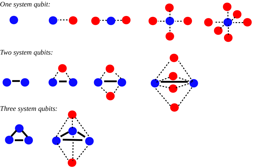
Figure 1: Configurations of system (blue) and noise (red) qubits studied in the non-Markovian case. Couplings between the noise qubits are neglected and system-system qubit couplings are assumed to be stronger than system-noise qubit couplings.

3 Optimal Control Theory & Algorithms

3.1 Discretisation and Optimisation Algorithm

We use model-based optimal control where an objective functional is defined and the control field is numerically optimised to obtain the best possible value of the functional. A canonical choice for the performance index for gate optimisation problems is the gate error $\mathcal{E}$. We discretise the controls $f_{m}(t)$ using piecewise constant functions, dividing the total time $T$ into $K$ slices $[t_{p-1},t_{p}]$ of duration $\Delta t=T/K$ and setting $f_{m}(t)=f_{mp}$ for $t\in[t_{p-1},t_{p}]$. Thus, we have

$$f_{m}(t)=\sum_{p=1}^{K}f_{mp}\chi_{p}(t),$$ (6)

where $\chi_{p}(t)=1$ for $t\in[t_{p-1},t_{p}]$ and $0$ elsewhere. This parameterisation is a common choice and natural for many applications such as nuclear magnetic resonance, where waveform generators can approximate a piecewise constant output. Other parameterisations may be considered as appropriate for other applications. After discretisation of the controls, we are left with a vector of control parameters $\mathbf{f}$ and an error functional $\mathcal{E}(\mathbf{f})$ and our goal is to find a control vector $\mathbf{f}_{*}$ such that $\mathcal{E}(\mathbf{f}_{*})$ assumes its global minimum.

Motivated by a recent comparison of various first- and second-order sequential and concurrent update methods [33], we opt for a concurrent update quasi-Newton method  , which involves iteratively updating the control parameters according to the Newton update rule,

$$\mathbf{f}^{(k+1)}=\mathbf{f}^{(k)}-\alpha_{k}(\mathbf{H}_{k})^{-1}\nabla\mathcal{E}(\mathbf{f}^{(k)}),$$ (7)

starting with a guess for the initial field $f^{(0)}$ and an initial Hessian approximation $\mathbf{H}_{0}$. The initial Hessian is taken to be the identity and the approximate Hessian is then constructed from the past gradient history according to the Broyden-Fletcher-Goldfarb-Shanno (BFGS) formula

$$(\mathbf{H}_{k})^{-1}=\left(1-\frac{\mathbf{g}_{k-1}\mathbf{s}_{k-1}^{\mathrm{T}}}{\mathbf{g}_{k-1}^{\mathrm{T}}\mathbf{s}_{k-1}}\right)(\mathbf{H}_{k-1})^{-1}\left(1-\frac{\mathbf{g}_{k-1}\mathbf{s}_{k-1}^{\mathrm{T}}}{\mathbf{g}_{k-1}^{\mathrm{T}}\mathbf{s}_{k-1}}\right)+\frac{\mathbf{s}_{k-1}\mathbf{s}_{k-1}^{\mathrm{T}}}{\mathbf{g}_{k-1}^{\mathrm{T}}\mathbf{s}_{k-1}},$$ (8)

where $\mathbf{s}_{k-1}=\mathbf{f}^{(k)}-\mathbf{f}^{(k-1)}$, $\mathbf{g}_{k-1}=\nabla\mathcal{E}(\mathbf{f}^{(k)})-\nabla\mathcal{E}(\mathbf{f}^{(k-1)})$, and $\alpha_{k}=1$ by default; $\alpha_{k}$ is the search length parameter for a standard Newton step.

The optimisation algorithm requires the computation of derivatives of the objective functional $\mathcal{E}=\mathcal{E}(f_{mp})$ with regard to the control variables $f_{mk}$. The simplest approach is to approximate the required derivatives numerically using finite differences [30],

$$\frac{\partial\mathcal{E}(f_{mp})}{\partial f_{mp}}=\lim_{\Delta f_{mp}\to 0}\left\{\frac{1}{\Delta f_{mp}}\left[\mathcal{E}(f_{mp}+\Delta f_{mp})-\mathcal{E}(f_{mp})\right]\right\},$$ (9)

with

$$\frac{\partial\mathcal{E}(f_{mp})}{\partial f_{mp}}\approx\frac{1}{\Delta f_{mp}}\left[\mathcal{E}(f_{mp}+\Delta f_{mp})-\mathcal{E}(f_{mp})\right],$$ (10)

for a finite value of $\Delta f_{mp}$. This calculation can be made efficient by recognising that the error does not need to be explicitly evaluated at the two different fidelities [31]. A serious drawback, however, is that the value of the step size is constrained by the fact that choosing too large a value renders the approximation invalid while choosing too small a value reduces the number of accurate digits of the difference in the floating point representation to zero [31]. The step-size parameter therefore needs to be chosen carefully. For the low-dimensional systems considered in the following, step sizes on the order of $10^{-6}$ generally gave good results, but the optimal value is usually not known a-priori and thus needs to be determined by trial and error.

To avoid this problem, analytical derivative formulae can be derived. For typical gate optimisation problems, the error function $\mathcal{E}(\mathbf{f})$ is a simple functional of the time evolution operator $X(t)$ of the system, and a derivation similar to [30] shows that for piecewise constant controls

$$\frac{\partial X(T)}{\partial f_{mp}}=X(T,t_{p})\left[\int_{t_{p-1}}^{t_{p}}X(t_{p},\tau)A_{m}X(\tau,t_{p-1})d\tau\right]X(t_{p-1}),$$ (11)

where $X(t,t_{p-1})=\exp[(t-t_{p-1})\mathcal{L}(f_{mp})]X(t_{p-1})$ and $\mathcal{L}(f_{mp})=\mathcal{L}_{0}+\mathcal{L}_{D}+\sum_{m}f_{mp}\mathcal{L}_{m}$ for general Markovian systems; in addition, $X(t,t_{p-1})=\exp[-i(t-t_{p-1})H(f_{mp})]X(t_{p-1})$ and $H(f_{mp})=H_{0}+\sum_{m}f_{mp}H_{m}$ for closed systems subject to unitary evolution. The latter case includes the non-Markovian systems discussed above if $H$ is taken to be the Hamiltonian and $X(t)$ the unitary evolution operator of the total system including the noise qubits. The integral in (11) can be evaluated exactly via the augmented matrix exponential formula

$$\exp\begin{pmatrix}A&B\\ 0&C\end{pmatrix}=\begin{pmatrix}e^{A}&\int_{0}^{1}e^{A(1-s)}Be^{Cs}\,ds\\ 0&e^{C}\end{pmatrix}$$ (12)

by setting $A=C=\mathcal{L}(f_{mp})\Delta t$ and $B=\mathcal{L}_{m}\Delta t$ or $A=C=-iH(f_{mp})\Delta t$ and $B=H_{m}\Delta t$. Thus we can compute both the matrix exponential $X(t_{p},t_{p-1})$ and the desired derivative simply by computing the matrix exponential of an augmented matrix twice the size of the system operators. If $\mathcal{L}(f_{mp})$ is diagonalisable, then the matrix exponential and gradient can alternatively be computed using the spectral decomposition of $\mathcal{L}(f_{mn})$ as discussed in [30]; spectral decomposition is usually the preferred approach for such systems.

For any Hamiltonian system, including closed systems and non-Markovian systems with noise qubits, the total Hamiltonian $-iH(f_{mp})$ is always skew-Hermitian and thus diagonalisable. The superoperators for most systems subject to Markovian non-unitary evolution, on the other hand, are often not diagonalisable. Therefore, the spectral decomposition approach is usually the preferred choice for closed and non-Markovian systems while the augmented matrix exponential is useful for other cases where accurate gradients are required. For small systems such as the one- and two-qubit Markovian systems considered below, the evaluation of the augmented matrix exponential was actually faster than using the finite difference approximation in our simulations. For higher dimensional systems, the evaluation of the augmented matrix exponential tends to be computationally more expensive than the computation of the gradient using the finite difference approximation. On the other hand, the analytic formula allows for more accurate gradient computations. Gradient accuracy is a significant factor for the performance of any type of algorithm using gradients, especially quasi-Newton methods, and previous work for closed systems has shown that low-order gradient approximations, even if they are faster to compute, are detrimental to the performance of the algorithm in terms of leading to poor convergence and lower fidelities, unless very small step sizes are used [31, 33]. Nonetheless, with carefully chosen finite difference step-sizes it was possible to achieve sufficient gradient accuracy to reproduce the convergence behaviour and final fidelities obtained using the augmented matrix exponential routine in most of our Markovian system simulations. For non-Markovian systems, the finite difference approximation was not used due to lack of any discernible benefit.

The algorithm also requires initial fields $\mathbf{f}^{(0)}$ to start the iteration. Here we choose the components of $\mathbf{f}^{(0)}$ by randomly sampling according to a Gaussian distribution with mean $0$ and standard deviation $\sigma(f_{m}^{(0)})=\delta$ where $\delta$ is a free parameter. $\|\mathbf{f}_{m}\|^{2}=\sum_{p=1}^{K}|f_{mp}|^{2}\approx K\delta^{2}$ shows that $\delta$ determines the norm of the initial field vector of each component field $\mathbf{f}_{m}^{(0)}=(f_{m1},\ldots,f_{mK})$. For piecewise constant functions with fixed $\Delta t$, the norm of the field vector is proportional to the $L^{2}$ norm of the field as a function over $[0,T]$:

$$\|\mathbf{f}_{m}(t)\|_{2}^{2}=\int_{0}^{T}|f_{m}(t)|^{2}dt=\Delta t\sum_{p=1}^{K}|f_{mp}|^{2}=\Delta t\|\mathbf{f}_{m}\|^{2}.$$ (13)

We refer to the square of the $L^{2}$ norm of a field as the fluence of the pulse, a quantity that is of independent physical interest as it is proportional to the pulse energy.

3.2 Explicit Error Functionals for the Markovian/Non-Markovian Case

For general Markovian dynamics, the most natural way to compare quantum processes is by considering the distance between the processes in the adjoint representation. The adjoint representation of a unitary target operator $W$ with respect to the chosen basis $\{\sigma_{k}\}$ is given by the $N_{1}^{2}\times N_{1}^{2}$ real matrix $Y$ with $Y_{mn}=\operatorname{Tr}(\sigma_{m}W\sigma_{n}W^{\dagger})$. Letting $X(t)$ be the real adjoint representations of the time-evolution operator of the system defined earlier, we can define the gate error in terms of the square of the Frobenius (or Hilbert-Schmidt) norm of $\Lambda(t)=Y-X(t)$,

$$\mathcal{E}_{1}^{\prime}=\lambda\operatorname{Tr}[\Lambda^{\mathrm{T}}(T)\Lambda(T)]=\lambda\left(\operatorname{Tr}(Y^{\mathrm{T}}Y)+\operatorname{Tr}[X(T)^{\mathrm{T}}X(T)]-2\operatorname{Tr}[Y^{\mathrm{T}}X(T)]\right),$$ (14)

where $\lambda$ is a scaling factor. The gate error is a simple functional of the evolution operator and thus

$$\frac{\partial\mathcal{E}_{1}^{\prime}}{\partial f_{mp}}=2\lambda\operatorname{Tr}\left[\Lambda^{T}(T)\frac{\partial\Lambda(T)}{\partial f_{mp}}\right]=-2\lambda\operatorname{Tr}\left[\Lambda^{T}(T)\frac{\partial X(T)}{\partial f_{mp}}\right],$$ (15)

where $\tfrac{\partial X(T)}{\partial f_{mp}}$ are the partial derivatives of the evolution operator as defined in (11). We will use this performance index with $\lambda=\tfrac{1}{2N_{1}^{2}}$ for the optimisation. However, for the sake of a direct error comparison with closed and non-Markovian systems, we also define the error functional

$$\mathcal{E}_{1}=1-\mathcal{F}_{1},\quad\mathcal{F}_{1}=\sqrt{1-\mathcal{E}_{1}^{\prime}},$$ (16)

where $\mathcal{F}_{1}$ is the unit gate fidelity. It is easy to check that this gate fidelity agrees with the gate fidelity for closed systems if the Lindblad operators vanish.

For non-Markovian systems, one may be tempted to simply define the gate error by

$$\mathcal{E}=1-\tfrac{1}{N}|\operatorname{Tr}[(W\otimes\mathbb{I})^{\dagger}X(T)]|,$$ (17)

where $N$ is the dimension, $X(T)$ the (unitary) time evolution operator of the composite system, $W$ the target operator on the system, and $\mathbb{I}$ the identity operator on the noise subsystem. However, this error vanishes only if we simultaneously implement the target gate $W$ on the system subsystem and the identity on the noise subsystem. Usually, however, we do not care what the evolution of the noise subsystem is. Therefore, a better measure of the gate error is

$$\mathcal{E}_{2}=\lambda\min_{\phi}\|W\otimes\phi-X(T)\|^{2},$$ (18)

where $\phi$ is an arbitrary time-evolution operator acting on the noise subsystem only, and $\lambda$ is a normalisation constant that can be chosen so that the error ranges between $0$ and $1$, for instance. Taking the matrix norm in (18) to be the Frobenius norm and setting $\lambda=\frac{1}{2N}$, it can be shown that [6, 32]

$$\mathcal{E}_{2}=1-\mathcal{F}_{2},\quad\mathcal{F}_{2}=\tfrac{1}{N}\operatorname{Tr}\sqrt{Q^{\dagger}Q},$$ (19)

where $Q=\operatorname{Tr}_{S}((W\otimes\mathbb{I})^{\dagger}X(T))$, $\operatorname{Tr}_{S}$ denotes the partial trace over the system $S$, and $\mathcal{F}_{2}$ is the gate fidelity. Differentiating (19) with respect to $f_{mp}$, we obtain

$$\frac{\partial\mathcal{E}_{2}}{\partial f_{mp}}=-\frac{1}{N}\mathrm{Re}\operatorname{Tr}\left(\frac{1}{\sqrt{Q^{\dagger}Q}}Q^{\dagger}\frac{\partial Q}{\partial f_{mp}}\right),\ \quad\frac{\partial Q}{\partial f_{mp}}=\operatorname{Tr}_{S}\left[(W\otimes\mathbb{I})^{\dagger}\frac{\partial X(T)}{\partial f_{mp}}\right],$$ (20)

and thus the gradient is again defined in terms of the partial derivatives of the total evolution operator $X(T)$ with regard to the control variables $f_{mp}$. $\sqrt{Q^{\dagger}Q}$ may become singular but from the singular value decomposition $Q=GDE^{\dagger}$, where $G$ and $D$ are unitary matrices and $D$ is a diagonal matrix with non-negative entries, one can easily verify that $(Q^{\dagger}Q)^{-1/2}Q^{\dagger}=EG^{\dagger}$, which can be defined even if $\sqrt{Q^{\dagger}Q}$ is singular.

4 Results and Discussion

To evaluate the performance of the algorithm and quality of the solutions found, we studied a variety of gate optimisation tasks for single, two-, and three-qubit systems in different Markovian and non-Markovian environments. Details of the system parameters chosen are given in Tables 1 and 2. In our system of units, $\hbar=\omega_{1}=|\mu_{1}|=k_{B}=1$, where $\omega_{1}$ is the angular frequency of the system qubit in the one-qubit case and $k_{B}$ is the Boltzmann constant. Throughout this paper time is expressed in units of $\omega_{1}^{-1}$. In addition to fundamental issues such as asymptotic error values, how rapidly we converge to these, and the dependence of the convergence behaviour and limiting values on algorithmic parameters such as the choice of the initial fields $\mathbf{f}^{(0)}$, we also considered the impact of unwanted side effects such as field leakage and analysed the characteristics of the optimal fields.

Table 1: Summary of the system parameters in the Markovian model

	1 system qubit	2 system qubits	3 system qubits
Decoherence type (emission / dephasing rate in units of $\omega_{1}$)	No decoherence Spontaneous emission (0.02) Independent dephasing in the z-basis (0.02) Independent dephasing in the x-basis (0.02)	No decoherence Spontaneous emission (0.02) Independent dephasing in the z-basis (0.02) Independent dephasing in the x-basis (0.02)	No decoherence Independent dephasing in the z-basis (0.02) Independent dephasing in the x-basis (0.02) Correlated dephasing in the z-basis (0.02)
Frequencies of system qubits (in units of $\omega_{1}$)	1	0.95 and 1.05	0.95, 1, and 1.05
Heisenberg coupling strength (in units of $\omega_{1}$)	1	1	1
Target gate(s)	Hadamard, Identity, T-gate	Identity, CNOT	3-qubit quantum Fourier transform (QFT), Identity
Target times in units of $\omega_{1}^{-1}$, (Time slices $K$)	5 (25), 25 (25)	25 (150), 50 (150), 75 (150), 100 (150)	150 (300)
Initial field std deviation	0.1, 1, or 10	0.01, 0.1, 1, or 10	1

Table 2: Summary of the non-Markovian systems analysed

	1 system qubit	2 system qubits	3 system qubits
Number of noise qubits	0, 1, 2, 4, or 6	0, 1, 2, or 4	0 or 2
Frequencies for system qubits (in units of $\omega_{1}$)	1	0.95 and 1.05	0.95, 1, and 1.05
Noise qubit frequencies (in units of $\omega_{1}$)	$(\pi-2.14)^{-1}$, $(\pi-2.14)$ $(\pi-2.1)^{-1}$, $(\pi-2.1)$ $(\pi-2)^{-1}$, $(\pi-2)$	$(\pi-2.14)^{-1}$, $(\pi-2.14)$ $(\pi-2.1)^{-1}$, $(\pi-2.1)$	$(\pi-2.14)^{-1}$, $(\pi-2.14)$
Heisenberg coupling strengh $\gamma$ (in units of $\omega_{1}$)	0.02 between system and noise qubits	0.1 between system qubits, 0.01 between system and noise qubits	0.1 between system qubits, 0.01 between system and noise qubits
Target gates	Hadamard, Identity, T-gate	Identity, CNOT	3-qubit quantum Fourier transform, Identity
Target times in units of $\omega_{1}^{-1}$, (time slices)	2 (25), 3 (25), 4 (25), or 25 (25)	25, 30, 35, 40, 45, 50, 55, 60, 65, 70, 75, 80, 85, 90, 95, 100, 125 (150 time slices each)	150 (300) or 300 (300)
Initial field std deviation	0.1, 1, or 10	0.01, 0.05, 0.1, 0.5, 1, 5, or 10	1

4.1 Convergence Behaviour and Asymptotic Error Values

Figure 2: Convergence behaviour

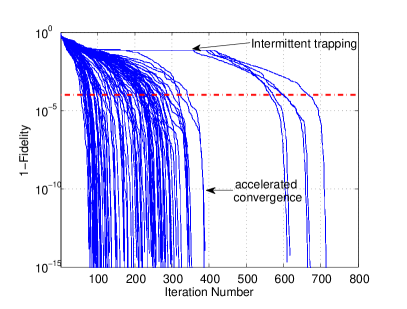
(a) Two-qubit CNOT gate, no decoherence, $T=75$ $\omega_{1}^{-1}$, $\sigma(f^{(0)})=0.1$

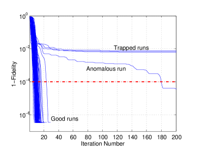
(b) One-qubit T gate, spontaneous emission, $T=5$ $\omega_{1}^{-1}$, $\sigma(f^{(0)})=0.1$

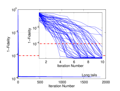
(c) One-qubit Had gate, $x$-dephasing, $T=5$ $\omega_{1}^{-1}$, $\sigma(f^{(0)})=10$

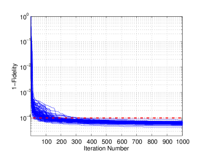
(d) One-qubit Had gate, two noise qubits, $T=3$ $\omega_{1}^{-1}$, $\|\mathbf{f}^{(0)}\|=10$

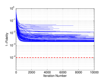
(e) Three-qubit QFT gate, spontaneous emission, $T=150$ $\omega_{1}^{-1}$, $\sigma(f^{(0)})=1$

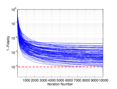
(f) Three-qubit QFT gate, two noise qubits, $T=300$ $\omega_{1}^{-1}$, $\|\mathbf{f}^{(0)}\|=1$

For simple problems, we found considerable uniformity in terms of the final values of the fidelities achieved for different runs and different target gates. For example, for the one- and two-qubit gate problems considered the final fidelities of more than 95% of all runs for a given problem typically agreed to three or more decimal places. This suggests that most runs converged to a control that achieved close to optimal performance in terms of reaching an error very close to the global minimum attainable for the given form of decoherence and control field restrictions (such as the field parameterisation, target time, and time resolution). This was the case in both the Markovian and non-Markovian case although the errors in the Markovian case were higher, especially for the more complex gates. For instance, for the three-qubit QFT gate the maximum asymptotic fidelity was around 99.8% for spontaneous emission, 99.3% for dephasing in either the $x$ or $z$ basis, and 99.2% for correlated $zz$-dephasing at a rate of $0.02$ for $T=150$, while errors $<10^{-4}$ were attainable for the non-Markovian cases. This is not unexpected considering that the Markovian setting lacks the possibility of coherence revivals. As the difficulty of the gate optimisation problems increased, however, far less uniform convergence behaviour and increasingly large spreads of final fidelities were observed, again in both the Markovian and non-Markovian cases. This is exemplified in Fig. 2 which shows the convergence behaviour for 100 runs each for different cases. For instance, the error of the best run in Fig. 2(f) was $<10^{-4}$ while the error of the worst run was $0.0043$, two orders of magnitude larger.

Conclusion 1: While for simple control tasks a single run with a randomly chosen initial field usually suffices, multiple runs with different initial conditions are essential to find a control that achieves the best possible fidelity for harder control problems.

An important difference in the convergence behaviour between open and closed systems is that in the latter we generally observed accelerated convergence as shown in Fig. 2(a), while in the dissipative case the convergence was at best linear as in Fig. 2(b) and, in most cases, we actually observed a slowdown in the rate at which the error decreased. Moreover, trapping and long tails are seen in the Markovian and non-Markovian cases. This behaviour is consistent with convergence to a limiting value of the error strictly greater than $0$, which is expected for open systems.

The accuracy of the gradient approximation is another limiting factor for very high fidelities. When quasi-Newton methods are used as in our case, the errors in the gradients will eventually also lead to large errors in the approximate Hessian and increasingly poor performance of the quasi-Newton iteration, precluding further reductions in the errors. The algorithm should be terminated before this regime is reached. The use of analytic gradient formulae can alleviate this problem. However, even the augmented matrix exponential or spectral decomposition gradient formulae, though theoretically exact, will be subject to numerical approximation errors in practice.

Conclusion 2: Trapping, long tails, and diminishing returns as a function of the iteration number for open systems make sensible termination conditions essential.

While for controllable closed systems it is often reasonable to set a threshold such as $-10^{-4}$ for the error as the termination condition, for open systems there are usually no strict upper bounds on the attainable fidelities and the best strategy therefore is to dynamically monitor the rate of decrease in the error and terminate the optimisation when this value becomes too low and we have reached an asymptotic regime.

4.2 Dependence on Gate Operation Time and Initial Fields

Assuming the model and objective have already been chosen, the algorithm depends on two key inputs: the gate operation time $T$ and the choice of the initial fields. An interesting question is how the choice of these parameters affects the convergence behaviour and limiting values of the fidelities attained. Initial test runs suggested a dependence of the convergence behaviour on the magnitude of the initial fields, which in our case was determined by the variance of the Gaussian distribution we sampled from. To better understand the effects of the target time and magnitude of the initial fields on the convergence behaviour and fidelities attained, we combined the data from many runs for initial fields with different norms (always sampled from a normal distribution) and different target times into 2D density plots for the success rate and the success speed. The success rate here is the fraction of runs for a given choice of initial field norm and target time that reached fidelities at or above the error threshold, which we set to be $10^{-4}$. The success speed was defined as the inverse of the expected time required to succeed in finding a control that achieves the desired error threshold, where the expected time to succeed is computed as [33]

$$\mbox{mean failed run time}\times\frac{\mbox{number of failed runs}}{\mbox{number of successful runs}}+\mbox{mean successful run time}.$$ (21)

Figure 3: Success rate plots for two-qubit system for error threshold $10^{-4}$ with colour bars indicating the success rate

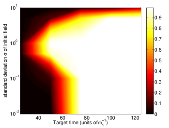
(a) Two-qubit CNOT gate (no noise qubits)

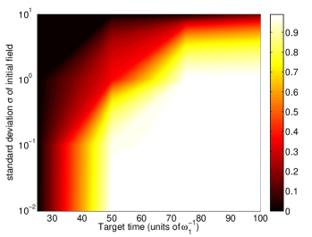
(b) Two-qubit Id gate (no noise qubits)

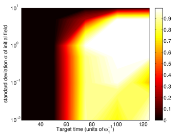
(c) Two-qubit CNOT gate (1 noise qubit)

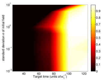
(d) Two-qubit Id gate (1 noise qubit)

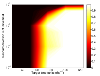
(e) Two-qubit CNOT gate (2 noise qubits)

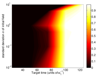
(f) Two-qubit Id gate (2 noise qubits)

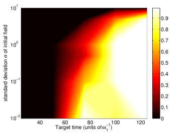
(g) Two-qubit CNOT gate (4 noise qubits)

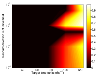
(h) Two-qubit Id gate (4 noise qubits)

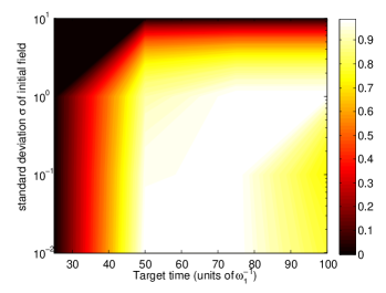
(i) CNOT gate, $z$-dephasing

(j) Two-qubit Id gate, $z$-dephasing

Figure 4: Success speed plots for two-qubit system for error threshold $10^{-4}$ with colorbars indicating success speed.

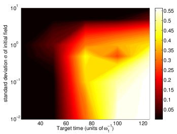
(a) Two-qubit CNOT gate(no noise qubits)

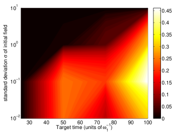
(b) Two-qubit Id gate (no noise qubits)

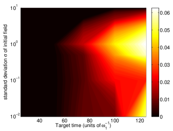
(c) Two-qubit CNOT gate (1 noise qubit)

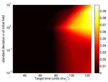
(d) Two-qubit Id gate (1 noise qubit)

(e) Two-qubit CNOT gate (2 noise qubits)

(f) Two-qubit Id gate (2 noise qubits)

(g) Two-qubit CNOT gate (4 noise qubits)

(h) Two-qubit Id gate (4 noise qubits)

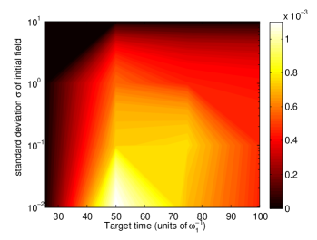
(i) CNOT gate, $z$-dephasing

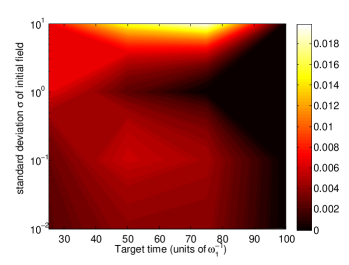
(j) Two-qubit Id gate, $z$-dephasing

For Markovian systems one expects that there exists an optimum time to implement a desired gate with the highest possible fidelity. This time is expected to depend on the details of the system and the Lindblad operators describing the effects of the bath. For shorter gate operation times, the fidelities will be lower due to a lack of time to implement the required control [35]; for longer times, decoherence effects will reduce the fidelity. For non-Markovian systems, there is generally no upper limit for the gate operation times and we expect longer times to improve both success rates and speeds. In fact, with a sufficiently long evolution time and no restrictions on the control fields, one can in theory always achieve perfect fidelities if the composite system evolves unitarily and is controllable, as is the case for our systems.

The success rate plots (Fig. 3) for both a CNOT and two-qubit identity gate do indeed suggest that there is a lower bound on the target time but no upper bound. Moreover, the success rate plots for one, two, and four noise qubits are very similar and the threshold value for the gate operation time increases only marginally when more noise qubits are added, especially for the CNOT gate. This suggests that neither the difficulty of finding a control nor the time required to implement the gate increases substantially when more noise qubits are added, a very desirable situation in practice. The picture is slightly less favourable for the identity gate in that the minimum time necessary to successfully implement the gate with the desired fidelity increases more significantly (from 40 in the absence of noise qubits to about 80 for one, two, or four noise qubits). In the Markovian case, Fig. 3(i) does show a slight decrease in the success rate for larger gate operation times for the CNOT gate, as expected based on the observation above. Nevertheless, much more interesting is the success rate plot for the identity Fig. 3(j), for which there appears to be no minimum gate operation time but there is a sharp drop in the success rate when $T$ gets too large.

For both models, the success rate plots for the CNOT gate show a sharp drop in the success probability regardless of the target time when the amplitudes of the initial fields get too large. The success speed plots (Fig.4) further suggest the existence of a sweet spot (white) with regard to the field amplitudes for which we can expect rapid convergence. For larger initial field amplitudes, we can expect poor performance due to trapping in sub-global extrema; for too small initial field amplitudes, we can expect slow convergence. It is therefore desirable to determine the optimum range of initial field amplitudes at the outset, which could be done by adapting the methodology which has been successful for closed systems [36]. In the non-Markovian setting the success speed plots for both the CNOT and identity gate are not too dissimilar; in particular, the success speed plots have a sweet spot for larger target times around a certain optimum value of the initial field amplitudes. In the Markovian setting, on the other hand, the shortest time to success was achieved for initial fields with a small magnitude for the CNOT gate but large magnitude for the identity gate, showing that the optimum initial field amplitudes may depend on the target gate to be implemented. In general, the identity gate was harder to implement with high fidelity than the CNOT. A given realization of a basic quantum information processor may thus be more effective in carrying out certain operations than others, and implementing a trivial gate may, in fact, be harder than implementing a maximally entangling gate.

4.3 Pre-optimised fields

Figure 5: Performance of pre-optimised fields and improvement when environment is taken into account.

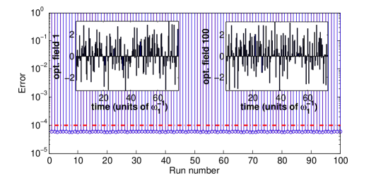
(a) 2 qubits, indep. $z$-dephasing, CNOT, $T=75$ $\omega_{1}^{-1}$

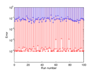
(b) 2 qubits, 4 noise qubits, CNOT, $T=75$ $\omega_{1}^{-1}$

Another interesting question is how important it is to take the effect of the environment into account when optimising the gate performance. In general, one expects a better performance when the environment is taken into account but this is computationally much more expensive. It is therefore informative to compare the performance of the fields optimised with and without taking the environment into account. To do this, we first optimise the controls neglecting decoherence and then start the iteration in the dissipative case with an optimal control obtained for the Hamiltonian case. Here, we observe major differences depending on the type of environment.

In the Markovian case the optimal fields obtained without the environment performed quite well — taking the decoherence mechanisms into account resulted in little, if any, improvement, as shown in Fig. 5(a). The blue stems in the figure indicate the error achieved when the pre-optimised fields are directly applied to the dissipative system, while the red stems indicate the final errors achieved when these fields are used as inputs for optimisation with decoherence. The red and blue stems are virtually indistinguishable which suggests that the performance of the optimal control fields obtained without considering decoherence is comparable to that obtained taking the Markovian environment into account. This was the case across the board for thousands of simulations for all of the systems, gates, and Markovian environments considered here. This disappointing performance of optimal control for Markovian systems may seem surprising in view of some earlier work but it is actually in line with results in [39] as substantial improvements in the fidelities achieved with optimal control in this work were observed only for a qubit encoded in a weakly relaxing subspace, a distinctly different situation from the one considered here. In general, the simulation results are consistent with the observations that open-loop coherent control cannot undo the effects of Markovian decoherence [8]. This should not be interpreted to imply that optimal control design is not useful for systems subject to Markovian decoherence. Optimal control generally still leads to more efficient quantum gates; however, there are fundamental limitations and it may be necessary to combine optimal control design with other strategies such as robust encoding of quantum information or feedback.

In the non-Markovian case, pre-optimised fields almost always performed poorly and the fidelities could be considerably improved by taking the noise qubits into account in the optimisation, as illustrated in Fig. 5(b). Note that we observe a reduction in the error by about three orders of magnitude. Starting with pre-optimised fields also did not improve the convergence speed or increase the attainable fidelities, compared to starting with random initial fields, suggesting that pre-optimisation is not beneficial in this case. The reason why the fields obtained without taking the noise qubits into account perform poorly can be seen if we plot the evolution of the Bloch vectors of the system and noise qubits. Fig. 6(a) shows the evolution of a single system qubit and four noise qubits under a field optimised to implement a HAD gate on the system qubit without taking the noise qubits into account. We see that although the field does not excite the noise qubits directly, they are indirectly excited due to the coupling to the system qubit. In addition, although the magnitude of the excitation is much less than that of the system qubit, it is sufficient to create entanglement between the system and noise qubits, reducing the length of the Bloch vector of the system qubit and the gate fidelity. When the noise qubits are taken into account in the optimisation, the algorithm finds a field that avoids indirect excitation of the noise qubits almost entirely, as shown in Fig. 6(b). Entanglement between the system and noise qubits in this case is negligible and the gate fidelity is restored.

Figure 6: Bloch sphere trajectory plots for 1 system qubit and 4 noise qubits.

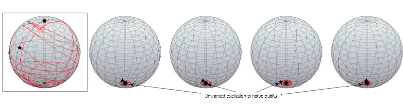
(a) Field optimised not taking noise qubits into account leads to unwanted excitation of noise qubits reducing the fidelity.

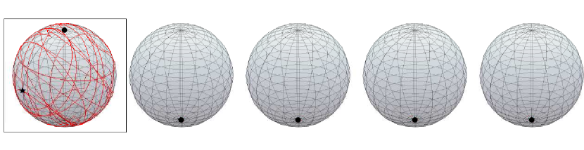
(b) Field optimized taking noise qubits into account suppresses excitation of noise qubits restoring fidelity.

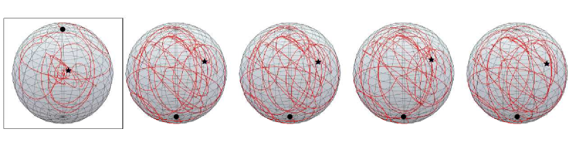
(c) Field optimised taking noise qubits into account fails to produce desired dynamics when noise qubits not shielded from field.

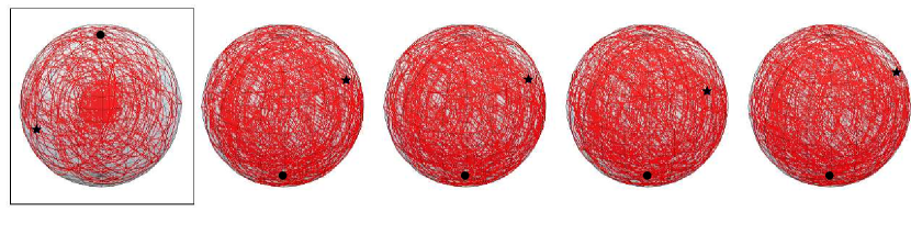
(d) Field optimised taking excitation of noise qubits into account can restore high fidelities by exploiting coherence revivals.

Initial and final states indicated by $\bullet$ and $\star$, respectively. First qubit (framed) is the system qubit. The gate operation time is $T=25$ $\omega_{1}^{-1}$ in the first three cases and $T=314$ $\omega_{1}^{-1}$ in the fourth case.

4.4 Control Mechanisms and Effects of Field Leakage

Figure 7: Effect of Field Leakage

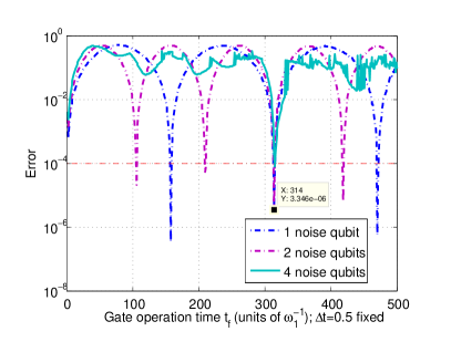
(a) HAD Gate error vs gate operation time $T$

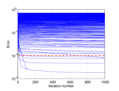
(b) Convergence for HAD gate with two noise qubits

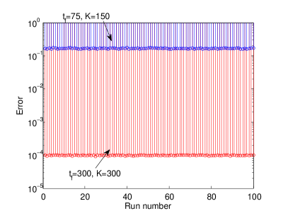
(c) Gate error for 2-qubit system with standard noise qubit

(d) Gate error for 2-qubit system with far-detuned noise qubit

In the previous calculations it was assumed that the noise qubits are shielded from the control field and that the field does not affect the environment in any way, an assumption that is not necessarily realistic. To assess the effect of field leakage we considered what happened if the noise qubits were affected by the fields as well — for example, due to field leakage. In the worst case scenario, the field seen by nearby noise qubits will be similar to that seen by the system qubits and they may interact with the field in a similar way to the system qubits. In this case, the final fidelities significantly decreased. In fact, the optimal fields obtained without considering the effect of the field on the noise qubits proved useless, as shown in the Bloch trajectory plot in figure 6(c). The noise qubits are now excited not only weakly by the coupling to the system qubit but also directly by the control field, resulting in significant excitation and entanglement between the system and noise qubits, evident by shrinkage of the length of the Bloch vector (especially for the system qubit). Nevertheless, if leakage is taken into account in the optimisation, the results can be improved, as shown in Fig. 6(d). We see that unlike in the no-leakage case (b), both the system and noise qubits are excited and now undergo complex evolutions. There is intermittent entanglement and the noise qubits are left in excited states at the final time; still, the field is such that the system qubit is disentangled from the noise qubits at the final time and the desired Hadamard gate is implemented.

However, to achieve such a performance, the gate operation time had to be substantially increased from $T=25$ to $T=314$ and chosen very carefully. When the target times and time resolution of the field were kept the same as before, the results were poor. Fig. 7(a) illustrates the complicated dependence of the attainable gate fidelities on the gate operation time for a single system qubit surrounded by multiple noise qubits with frequencies very close to the system qubit’s frequency. Only a few runs in Fig. 7(b), corresponding to the dips seen in Fig. 7(a), reach the error threshold of $10^{-4}$ but these successful runs usually reach it in relatively few iterations. Due to the rapid flattening out of the trajectories, most runs could have been terminated after fewer iterations as it is evident that they will not attain high fidelities. The significant increase in the amount of time needed to implement a simple single qubit gate can be explained in terms of global control. When the field leakage is taken into account, the control problem becomes a global control problem for a five qubit system and the only way we can achieve selective excitation of a single qubit is by exploiting the differences in the resonance frequencies of the qubits. Since frequency differences between the system and noise qubits are small in our case, more time is required to achieve selectivity. This suggests that the effect of leakage should be significantly reduced if the resonance frequencies of the noise qubits are significantly different from those of the system qubits.

To test this latter idea, we performed additional runs for a two-qubit system with one standard noise qubit, and the same system with a far-detuned noise qubit with $\Delta\omega=5$ instead. For our standard noise qubit, Fig. 7(c) shows that the gate errors for the two-qubit CNOT gate for $T=75$ and $K=150$ are large (blue stems). The gate operation times and time resolution of the field need to be increased substantially to achieve gate errors below $10^{-4}$ (red stems). However, Fig. 7(d) demonstrates that for a far-detuned noise qubit all 100 runs for $T=75$ and $K=150$ (and standard deviation of the initial fields equal to 1) reached the error threshold of $10^{-4}$ even when the noise qubit was not shielded, provided the effects of the fields on the noise qubit were taken into account in the optimisation. Accordingly, shielding the noise qubits from the control field may not be necessary, provided they are sufficiently detuned from the system qubit frequencies. This suggests that increasing the detuning of the noise qubits from the system qubits could be one way to mitigate the effect of the control fields on the noise qubits if leakage is unavoidable. For instance, this could be achieved via control electrodes [34] acting on the noise qubits (although in practice such direct control of the noise qubits could be technologically challenging). In this case, if the noise qubit frequencies are too similar to the system qubit frequencies and they cannot be shielded, high fidelities and good gate operation times may be out of reach even with the best optimal control.

4.5 Characteristics of the Optimal Fields

While finding solutions that achieve high fidelities is crucial and optimising the algorithms and parameters to achieve rapid convergence is highly desirable, not all optimal control solutions are created equal. In practice, the feasibility of the implementation of a control depends on its basic characteristics such as its pulse energy, amplitude, and bandwidth. Generally, fields with lower amplitudes and pulse energies are desirable as strong fields can be more difficult to implement and cause unwanted excitations or may even break the model the optimisation is based on.

In the Markovian case, analysis of the maximum field amplitudes of a large number of successful runs, that is, runs that achieved gate errors $<10^{-4}$, revealed a strong correlation with the magnitude of the initial fields, as determined by the standard deviation $\delta$ of the Gaussian distribution we sample from. This can be seen in the histogram plots of the maximum field amplitudes for 100 successful runs, for different values of the standard deviation of the initial fields (Fig. 8). In particular, low-amplitude initial fields ($\delta$ small) produce a narrow distribution with a small median value, meaning we are likely to converge to a low-amplitude field if we start with an initial field with a small amplitude. Accordingly, there is no need for the addition of penalty terms to the objective functional to constrain the field amplitudes. Penalty terms are generally undesirable as they prevent the algorithm from converging to a global optimum of the objective function and lead to slower convergence. In some cases — for example, Fig. 8(b) — the distribution has a long tail, that is, there are some runs starting with small fields that nonetheless converge to high-amplitude solutions. However, the probability of this happening is generally small, and if we do converge to a field with unexpectedly large amplitudes, we can most likely find a better solution by repeating the unconstrained optimisation with another suitably low-amplitude initial field.

In the non-Markovian case, we observe similar behaviour but the maximum field amplitude histograms tend to be less sharply peaked than in the Markovian case and can exhibit multi-modal features as in Fig. 8(d). In some cases, we also observe scattered outliers, which are fields with maximum amplitudes orders of magnitude greater than the median of the distribution, as shown in Fig. 8(c). In this setting, there can be substantial differences in the amplitudes of the optimal fields for initial fields with the same standard deviation; furthermore, the maximum amplitudes and energies of the optimal fields can be substantially reduced by running the algorithm several times to find a solution belonging to the lowest amplitude peak.

We also studied the correlations between the initial and final field fluences. As shown in Fig. 9, for large initial fluences, the final fluences cluster around large values that appear to be proportional to the initial fluence. For initial fluences below a certain value, the distribution of final fluences stabilises, so that we cannot decrease the fluence of the optimal fields below a certain threshold regardless of how small we choose the initial fluences. One way to explain this behaviour is that there is a certain minimum energy required to achieve the control objective. If we start with initial fields with energies (fluences) well below this value, the algorithm has to increase the field energy at least until we reach the minimum energy required to achieve the control objective. If we start with fields well below this minimum energy threshold, it may take many iterations to reach a regime where optimal controls exist, thus increasing the time required to find a solution. On the other hand, if we start with fluences well above the minimum required to achieve the control objective, the algorithm has no pressure to decrease the field energy – as we impose no penalty on the field fluences or amplitudes – and thus is likely to converge to an undesirable high-energy pulse. There is thus a best value for the variance of the initial fields to encourage rapid convergence to a low-energy optimal field.

Figure 8: Distribution of maximum amplitudes of optimal fields for different initial field amplitudes: $\delta=0.1$ (blue), $1$ (red) and $10$ (green) ($T$ in units of $\omega_{1}^{-1}$)

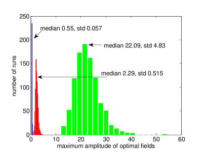
(a) Had gate, spontaneous emission, $T=25$

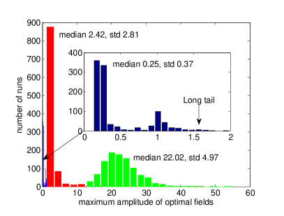
(b) Id gate, spontaneous emission, $T=25$

(c) Had gate, 1 qubit, 2 noise qubits, $T=25$

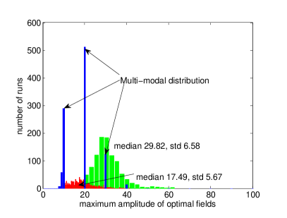
(d) Had gate, 1 qubit, 2 noise qubits, $T=3$

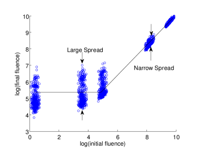
Figure 9: Scatter plot of the fluences of the converged fields versus the fluences of the initial fields for a two-qubit CNOT gate with 4 noise qubits.

5 Summary and Conclusions

We have presented a general framework for optimal control of quantum processes for systems in Markovian and non-Markovian environments. By suitable discretisation of the fields, we can reduce the complexity of the simulations and obtain analytic gradient formulae that enable us to apply efficient gradient-based optimisation algorithms such as second order quasi-Newton methods. To better understand the performance of the algorithms and the influence of parameters such as gate operation times and initial fields, we introduced new notions of success rates and speeds and used density plots as a new investigative tool. Using these tools combined with convergence and statistical analyses of basic characteristics of the optimal fields, we have investigated the reliability and efficiency with which optimally controlled quantum gates can be implemented on one, two, and three system qubits in Markovian and non-Markovian models. Although both models are based on rather different assumptions, the results for the control optimisation share some similarities.

First, the success rate and speed plots show that both the target gate operation times and magnitudes of the initial fields have a significant impact on the success rates and the expected times to succeed. For non-Markovian systems, however, the need to exploit coherence revivals can lead to a complex dependence of the attainable fidelities on the target times especially when the noise qubits are not shielded from the control and have similar frequencies as the system qubits. The success rate and speed plots also suggest that starting with too large field amplitudes increases the likelihood of trapping in many cases, and an analysis of the amplitude distributions for the optimal fields obtained shows that it can also lead to convergence to generally undesirable high-energy optimal fields. Too small amplitudes, on the other hand, tend to result in a slow convergence. It is therefore desirable to determine the optimum range of the initial field amplitudes, based on knowledge of the actual physical system under consideration [36].

Performing several optimisation runs for different initial fields is advantageous in all regimes considered. In the non-Markovian case, due to the spread of asymptotic fidelity values, more than one attempt may be needed to obtain a suitably low error solution. With no environment, a run which suffers from severe slowdown, even if only intermittently, can be abandoned in favour of starting a fresh run having a lower expected time to completion. In the Markovian case, both of these reasons apply and it is even more obvious than for non-Markovian systems that termination conditions are needed to avoid wasting time on the long tails observed in the convergence plots. Another reason to perform several runs is the considerable variability in the average and maximum amplitudes of the optimal fields across runs. This issue can also be addressed by imposing constraints during the optimisation procedure, in contrast to adding penalty terms to the objectives (which should be avoided since they limit the reachable fidelities [30]).

However, there are also significant differences in the results for the two models. Although optimal control is beneficial to find efficient solutions in both cases, in the Markovian setting the potential for optimal control is significantly reduced as the control cannot undo the effects of the environment, at least not if we are limited to open-loop coherent control. In that case, the benefits of optimal control are mainly the ability to implement operations faster or to reduce the detrimental effects of the environment by taking advantage of low-decoherence subspaces (if these exist). Results showing longer target times to be detrimental in the Markovian setting, at least in the absence of low-decoherence subspaces, support this conclusion. Perhaps the most surprising result of our simulations, however, is that the fields optimised without taking the environment into account still seemed to be optimal in the Markovian setting, at least if the decoherence is relatively uniform and sufficiently weak to be considered a perturbation of the Hamiltonian evolution. This was the case for all of the thousands of runs performed for single, two-, and three-qubit gates and various initial conditions. Furthermore, the simulations strongly suggest that the precise type of Markovian environment is not particularly important in that the fields that were optimal for independent dephasing in the $x$-basis achieved virtually the same performance for dephasing in the $z$-basis. Interestingly, independent relaxation (spontaneous emission) of the same strength was slightly less detrimental to the gate fidelities while correlated dephasing proved slightly more detrimental for the multi-qubit gates. These results contrast with earlier work [7] and suggest that more work is necessary to understand the mechanisms of action and fundamental limitations of optimal open-loop coherent control in the Markovian setting.

The situation is very different in the non-Markovian setting. In this case, the control, even if its action is limited to the system, can fully take advantage of memory effects in the environment to restore coherence to and decouple the system from the environment, given sufficient time and control strength. In contrast to the Markovian case, longer gate operation times are actually advantageous and accurate knowledge of the system-bath coupling is crucial. While in the Markovian case knowledge of the effective strength and uniformity of environmental effects is sufficient (and there is no need to know the precise type of coupling), fields optimised without taking the system-bath coupling into account, or optimised for a different type of bath, tend to perform poorly in the non-Markovian setting. This is consistent with earlier observations in the literature and suggests the need for accurate characterisation of the system-bath coupling. Further work is necessary to precisely quantify the degree of knowledge that is required. The Bloch trajectory analysis of a subset of the simulations further suggests that the fields optimised taking the system-bath coupling into account mainly act by manipulating the system as needed while at the same time decoupling it from and thus preventing excitation of the bath. Specific to the non-Markovian model, field leakage proved to be a major problem: the final fidelities decreased significantly when the field also acted on the noise qubits and optimal fields obtained without considering this effect proved effectively useless. More importantly, to restore high fidelities in the presence of field leakage generally required substantial increases in the gate operation times unless the frequencies of the noise qubits differed significantly from those of the system qubits. The mechanisms of action of the controls also shifted from suppression of bath excitation — now no longer possible — to exploiting interference effects to effectively disentangle the system and bath at the target time, while permitting substantial entanglement between system and bath at intermediate times. This suggests that field leakage is an important issue in practice that requires further study.

References

References

- [1] Zurek W H 1991 Phys. Today 44, 36–44
- [2] Palma M, Suominen K-A and Ekert A K 1996 Proc. R. Soc. Lond. A 452, 567–584
- [3] Viola L and Lloyd S 1998 Phys. Rev. A 58 2733–2744
- [4] Grace M, Brif C, Rabitz H, Walmsley I A, Kosut R and Lidar D 2006 New J. Phys. 8 35
- [5] Mancini S and Bonifacio R 2001 Phys. Rev. A 64 042111
- [6] Grace M, Brif C, Rabitz H, Walmsley I A, Kosut R L and Lidar D A 2007 J. Phys. B At. Mol. Opt. Phys. 40 102–125
- [7] Rebentrost P, Serban I, Schulte-Herbrüggen T and Wilhelm F K 2009 Phys. Rev. Lett. 102 090401
- [8] Solomon A I and Schirmer S G 2011 J. Russian Laser Research 32(5) 212
- [9] Golub J E and Mossberg T W 1986 JOSA B 3 554-559
- [10] D’Helon C and Milburn G J 1997 Phys. Rev. A 56 640-644
- [11] Dalvit D A R, Dziarmaga J and Zurek W H 2000 Phys. Rev. A 62 013607
- [12] Li B, Hazeltine R D, and Gentle K W 2007 Phys. Rev. E 76 066402
- [13] Lindblad G 1976 Comm. Math. Phys. 48 119-130
- [14] Wang X and Schirmer S G 2009 Phys. Rev. A 79 052326
- [15] Alicki R and Lendi K, Quantum Dynamical Semigroups and Applications (Springer, 2007)
- [16] Budini A A 2009, Phys. Rev. A 79 043804
- [17] Hartmann L, Calsamiglia J, Durr W and Briegel, H-J 2005 Phys. Rev. A 72 052107
- [18] Huebl H, Hoehne F, Grolik B, Stegner A R, Stutzmann M and Brandt M S 2008, Phys. Rev. Lett. 100 177602
- [19] Vaz E and Kyriakidis J 2010 Phys. Rev. B 81 085315
- [20] Eckel J, Weiss S, and Thorwart M 2006 Eur. Phys. J. B 53 91-98
- [21] Meunier T, Gleyzes S, Maioli P, Auffeves A, Nogues G, Brune M, Raimond J M and Haroche S 2005 Phys. Rev. Lett. 94 010401
- [22] Blockley C A, Walls D F and Risken H 1992 Europhys. Lett. 17 509-514
- [23] Brif C, Rabitz H, Wallentowitz S and Walmsley I A 2001 Phys. Rev. A 63 063404
- [24] Wallentowitz S, Walmsley I A, Waxer L J, and Richter Th. 2002 J. Phys. B: At. Mol. Opt. Phys. 35 1967-1984
- [25] Budini A A and Schomerus H 2005 J. Phys. A: Math. Gen. 38 9251-9262
- [26] Hwang B and Goan H-S 2012. Phys. Rev. A 85, 032321
- [27] Schmidt et al. 2011. Phys. Rev. Lett 107, 130404
- [28] Benenti G and Palma M 2007 Phys. Rev. A 75 052110
- [29] Grace M D, Brif C, Rabitz H, Lidar D A, Walmsley I A and Kosut R L 2007 J. Mod. Optics 54 2339-2349
- [30] Schirmer S G and de Fouquieres P 2011 New J. Phys. 13 073029
- [31] de Fouquieres P, Schirmer S G, Glaser S J and Kuprov I 2011 J. Magn. Res. 212 412
- [32] Kosut R L, Grace M, Brif C and Rabitz H 2006. http://arxiv.org/abs/quant-ph/0606064.
- [33] Machnes S, Sander U, Glaser S J, de Fouquieres P, Gruslys A, Schirmer S G, Schulte-Herbrueggen T 2011 Phys. Rev. A 84 022305
- [34] Nigmatullin R and Schirmer S G 2009 New J. Phys. 11 105032
- [35] Jurdjevic V and Sussmann H J 1972 J. Diff. Eq. 12 313-329
- [36] de Fouquieres P 2011. arXiv:1202.2530
- [37] Barreiro J T, Müller M, Schindler P, Nigg D, Monz T, Chwalla M, Hennrich M, Roos C F, Zoller P and Blatt R 2011 Nature 470 486-491
- [38] Wang X and Schirmer S G 2010. arXiv:1005.2114
- [39] Schulte-Herbrüggen T, Spörl A, Khaneja N and Glaser S J 2011, J. Phys. B: At. Mol. Opt. Phys. 44 154013