Detection with the scan and the average likelihood ratio

Abstract

We investigate the performance of the scan (the maximum likelihood ratio statistic) and of the average likelihood ratio statistic in the problem of detecting a deterministic signal with unknown spatial extent in the prototypical univariate sampled data model with white Gaussian noise. Our results show that the scan statistic, a popular tool for detection problems, is optimal only for the detection of signals with the smallest spatial extent. For signals with larger spatial extent the scan is suboptimal, and the power loss can be considerable. In contrast, the average likelihood ratio statistic is optimal for the detection of signals on all scales except the smallest ones, where its performance is only slightly suboptimal. We give rigorous mathematical statements of these results as well as heuristic explanations that suggest that the essence of these findings applies to detection problems quite generally, such as the detection of clusters in models involving densities or intensities, or the detection of multivariate signals. We present a modification of the average likelihood ratio that yields optimal detection of signals with arbitrary extent and which has the additional benefit of allowing for a fast computation of the statistic. In contrast, optimal detection with the scan seems to require the use of scale-dependent critical values.

Keywords and phrases. Scan statistic, average likelihood ratio statistic, optimal detection, fast algorithm.

AMS 2000 subject classification. 62G08, 62G10

^∗ Work supported by NUS grant R-155-000-090-112.
^∗∗ Work supported by NSF grant DMS-1007722 and NIH grant AI077395.

1 Introduction and overview of results

We are concerned with the problem of detecting a deterministic signal with unknown spatial extent against a noisy background. This problem arises in a wide range of applications, e.g. in epidemiology and astronomy, and has received considerable attention recently due to important problems in e.g. biosurveillance. The standard statistical tool to address this problem is the scan statistic (maximum likelihood ratio statistic), that considers the maximum of local likelihood ratio statistics on certain subsets of the data. There is a large body of work on scan statistics, see e.g. the references in Glaz and Balakrishnan (1999), Glaz, Naus, and Wallenstein (2001), and Glaz, Poznyakov, and Wallenstein (2009). But there is also empirical evidence that the scan statistic is suboptimal, see e.g. Neill (2009) or Chan (2009).

Siegmund (2001) and Gangnon and Clayton (2001) propose to use the average of the likelihood ratio statistics instead of their maximum. In different contexts, various versions of the average likelihood ratio where considered by Shiryaev (1963), Burnashev and Begmatov (1990), and Dümbgen (1998). Chan (2009) and Chan and Zhang (2009) perform simulation studies for various detection problems which suggest that the average likelihood ratio statistic is superior to the scan statistic. In light of these results, it is of interest to provide a theoretical investigation of the performance of both the scan and the average likelihood ratio. Such a theoretical comparison seems to be missing in the literature and appears to be quite relevant given the widespread use of the scan statistic as a standard tool for a range of detection problems.

In the first part of this paper we show that in the prototypical univariate sampled data model with white Gaussian noise the scan statistic possesses optimal detection power only for signals with the smallest spatial extent; otherwise the scan statistic is suboptimal, and the loss of power can be considerable for signals having a large spatial extent. We also show that for average likelihood ratio (ALR) statistic these conclusions hold in reversed order: The ALR possesses optimal detection power for signals having large spatial extent, but is suboptimal for signals with small spatial extent. However, the loss of power in the latter case is so small that it is unlikely to be of concern, at least for most sample sizes considered today.

In the second part of the paper we propose a modification of the ALR that results in universal optimality and allows efficient computation. The ALR averages the likelihood ratios pertaining to $\sim n^{2}$ stretches of the data, where $n$ is the sample size, resulting in an $O(n^{2})$ algorithm. Thus the use of the ALR is computationally infeasible even for moderate sample sizes. We introduce a condensed ALR that averages only a certain subset of the likelihood ratios and we show that this condensed ALR possesses optimal detection power for signals having arbitrary spatial extent. Furthermore, this condensed ALR can be computed in almost linear time, viz. with an $O(n\log^{2}n)$ algorithm. In light of the preceding discussion, it is arguably this improvement in computation time rather than the small gain in detection power that is the main advantage of this modification. We note that typically, an approximation introduced to make a procedure computationally less intensive will on the flip side degrade its performance somewhat. It is noteworthy that in the case of the ALR, our computationally efficient modification actually leads to an improved (in fact: optimal) performance.

We give sharp theoretical results on the performance of the ALR, the scan statistic, and the newly proposed ALR in Sections 2 and  3. Since these results are asymptotic, we complement them in Section 5 with a simulation study that illustrates the results. Various modifications to the scan have been proposed in the literature in order to improve its detection power. We describe two such modifications in Section 4, and include them in our simulation study to obtain a more informative comparison with the ALR.

As in the case of the ALR, the computation of the scan statistic requires an $O(n^{2})$ algorithm. Various efficient algorithms for computing a good approximation to the scan statistic have been introduced in Neill and Moore (2004), Arias-Castro, Donoho, and Huo (2005), Walther (2010) and Rufibach and Walther (2010). Unlike the ALR, constructing a computationally efficient approximation for the scan does not lead to universally optimal power. Rather, statistical optimality for the scan seems to require the use of size-dependent critical values. We summarize our conclusions in Section 6 and defer proofs to Section 7. The notation $a_{n}\sim b_{n}$ means $c<a_{n}/b_{n}<C$ for constants $0<c<C$.

2 Comparison of the scan and the average likelihood ratio

We observe

$$Y_{i}\ =\ f_{n}\Bigl{(}\frac{i}{n}\Bigr{)}+Z_{i},\ \ \ \ i=1,\ldots,n,$$

where the $Z_{i}$ are i.i.d. $N(0,1)$ and $f_{n}(x)=\mu_{n}{\bf 1}_{I_{n}}(x)$ with $I_{n}=(\frac{j_{n}}{n},\frac{k_{n}}{n}]$, $0\leq j_{n}<k_{n}\leq n$. Both the amplitude $\mu_{n}$ and the support $I_{n}$ are unknown. The task is to decide whether a signal is present, i.e. whether $\mu_{n}\neq 0$.

The above sampled data model with Gaussian white noise serves as a prototype for many important applications. The heuristics and results we develop below suggest that our conclusions carry over, at least qualitatively, to related detection problems involving multivariate signals, non-Gaussian errors, or the detection of clusters in models involving densities or intensities, as described in Kulldorff (1997).

The likelihood ratio statistic for testing $\mu_{n}=0$ when $I_{n}$ is known is computed as

$$\exp\Bigl{(}\frac{(\boldsymbol{Y}\!_{n}(I_{n}))^{2}}{2}\Bigr{)},\ \ \ \mbox{ where }\boldsymbol{Y}\!_{n}(I_{n}):=\frac{\sum_{i\in nI_{n}}Y_{i}}{\sqrt{n|I_{n}|}}=\frac{\sum_{i=j_{n}+1}^{k_{n}}Y_{i}}{\sqrt{k_{n}-j_{n}}}.$$

Since $I_{n}$ is unknown, the standard approach is to scan over all intervals $I\in{\cal J}_{n}:=\{(\frac{j}{n},\frac{k}{n}],0\leq j<k\leq n\}$ for the largest likelihood ratio statistic. The resulting scan statistic (maximum likelihood ratio statistic) is

$$M_{n}\ :=\ \max_{0\leq j<k\leq n}\Bigl{|}\boldsymbol{Y}\!_{n}\Bigl{(}\Bigl{(}\frac{j}{n},\frac{k}{n}\Bigr{]}\Bigr{)}\Bigr{|}.$$

In contrast, the average likelihood ratio statistic (ALR) averages the likelihood ratios over all intervals $I\in{\cal J}_{n}$:

$$A_{n}\ :=\ \frac{1}{n^{2}}\sum_{j=0}^{n}\sum_{k=j+1}^{n}\exp\Bigl{(}\frac{(\boldsymbol{Y}\!_{n}((\frac{j}{n},\frac{k}{n}]))^{2}}{2}\Bigr{)}.$$

To quantify the performance of these statistics, we look for the smallest value of $|\mu_{n}|$ that allows a reliable detection of the signal. As explained below, in order to achieve optimality a test must be able to asymptotically detect signals $f_{n}$ with

(1) $$|\mu_{n}|\sqrt{|I_{n}|}\ \geq\ \frac{\sqrt{2\log\frac{1}{|I_{n}|}}+b_{n}}{\sqrt{n}},\ \ \ \mbox{ where }b_{n}\rightarrow\infty.$$

Note that for signals $f_{n}$ on small scales, $|I_{n}|\rightarrow 0$, (1) is equivalent to

(2) $$|\mu_{n}|\sqrt{|I_{n}|}\ \geq\ (\sqrt{2}+\epsilon_{n})\sqrt{\frac{\log\frac{1}{|I_{n}|}}{n}},$$

where $\epsilon_{n}$ can go to 0 but not too fast: $\epsilon_{n}\sqrt{\log\frac{1}{|I_{n}|}}\rightarrow\infty$.

For signals $f_{n}$ on large scales, $\liminf_{n}|I_{n}|>0$, (1) is equivalent to

(3) $$|\mu_{n}|\ \geq\ \frac{b_{n}}{\sqrt{n}},\ \ \ \mbox{ where }b_{n}\rightarrow\infty.$$

It is impossible to detect signals with noticeably smaller mean: In the case of signals on small scales, a classical argument in the minimax framework (see e.g. Lepski and Tsybakov (2000), Dümbgen and Spokoiny (2001), and Dümbgen and Walther (2008)) shows that if ‘$+\epsilon_{n}$’ is replaced by ‘$-\epsilon_{n}$’ in (2), then there exists no test that can detect such $f_{n}$ with nontrivial asymptotic power. Likewise, a contiguity argument, as in Dümbgen and Walther (2008), shows that in the case of large scales the condition (3) is necessary for any test to be consistent against $f_{n}$. On the other hand, we exhibit below a test that detects signals satisfying (1) with asymptotic power 1. Thus the detection threshold given by (1) marks a standard that is attainable but cannot be improved upon. We now examine how the scan and the ALR compare against this standard.

Theorem 1

Let $\kappa_{n}$ be the $(1-\alpha)$ quantile of the null distribution of $M_{n}$.

1. If $|\mu_{n}|\sqrt{|I_{n}|}\geq(\sqrt{2}+\epsilon_{n})\sqrt{\frac{\log n}{n}}$ with $\epsilon_{n}\sqrt{\log n}\rightarrow\infty$, then ${\rm I\!P}_{f_{n}}(M_{n}>\kappa_{n})\rightarrow 1$.

2. If $|\mu_{n}|\sqrt{|I_{n}|}=(\sqrt{2}-\epsilon_{n})\sqrt{\frac{\log n}{n}}$ with $\epsilon_{n}$ as above, then $\overline{\lim}_{n}{\rm I\!P}_{f_{n}}(M_{n}>\kappa_{n})\leq\alpha$.

Thus the detection threshold for the scan is $\sqrt{2\frac{\log n}{n}}$, irrespective of the spatial extent of the signal. Comparing to (2), one sees that the scan is optimal only for signals having the smallest spatial extent, i.e. for $|I_{n}|$ close to $\frac{1}{n}$. As an illustration, if $|I_{n}|=n^{-p}$, $p\in(0,1]$, then detection is possible only if $|\mu_{n}|\sqrt{|I_{n}|}$ is at least $p^{-1/2}$ times larger than the optimal threshold. In the case of large scales, comparison with (3) shows that this multiplier diverges to infinity, and thus the scan suffers from a noticeably inferior performance. These results are illustrated in the simulation study in Section 5, and explain the sometimes disappointing performance of the scan observed in the literature.

We note that an alternative way to analyze the performance of the scan is to put a prior on the unknown spatial extent of the signal, e.g. the uniform distribution on $(0,1)$. It is readily seen that this analysis leads to the same conclusions as the case of large scales above, i.e. the scan is far from optimal.

The next theorem details the performance of the average likelihood ratio:

Theorem 2

Let $\tau_{n}$ be the $(1-\alpha)$ quantile of the null distribution of $A_{n}$.

1. $A_{n}$ is optimal for detecting signals with large spatial extent:
   If $\liminf_{n}|I_{n}|>0$ and $|\mu_{n}|=\frac{b_{n}}{\sqrt{n}}$ with $b_{n}\rightarrow\infty$, then ${\rm I\!P}_{f_{n}}(A_{n}>\tau_{n})\rightarrow 1$.

2. $A_{n}$ is not optimal for detecting signals with small spatial extent:
   If $|I_{n}|\rightarrow 0$ and $|\mu_{n}|\sqrt{|I_{n}|}=K\sqrt{\frac{\log\frac{1}{|I_{n}|}}{n}}$ with $K<2$, then $\overline{\lim}_{n}{\rm I\!P}_{f_{n}}(A_{n}>\tau_{n})\leq\alpha$.

3. If $K\geq 2+\epsilon_{n}$, where $\epsilon_{n}\sqrt{\log\frac{1}{|I_{n}|}}\rightarrow\infty$, then ${\rm I\!P}_{f_{n}}(A_{n}>\tau_{n})\rightarrow 1$.

Comparing with (2), one sees that on small scales the ALR requires $|\mu_{n}|\sqrt{|I_{n}|}$ to be about $\sqrt{2}$ times larger than the optimal threshold. This discrepancy is not very consequential: The simulations in Section 5 show that the corresponding loss of power is quite small for sample sizes up to $n=10000$, which is the largest sample size we were able to simulate due to the $O(n^{2})$ computational complexity of the ALR.

A heuristic explanation of why the scan and the ALR do not obtain optimality is as follows: There are $n$ disjoint intervals $I$ of length $1/n$. The corresponding likelihood ratio statistics $\boldsymbol{Y}\!_{n}(I)$ are i.i.d. N(0,1) under the null hypothesis, thus their maximum behaves like $\sqrt{2\log n}$. But in the case of large intervals of length $1/c$ (say), there are only $c$ disjoint intervals that result in independent statistics $\boldsymbol{Y}\!_{n}(I)$. The statistics for the other intervals of length $1/c$ are not independent of these $\boldsymbol{Y}\!_{n}(I)$ since the intervals overlap. Thus the null distribution of that maximum behaves roughly like the maximum of $c$ i.i.d. N(0,1), which is $O_{p}(1)$. Hence the overall maximum $M_{n}$ is dominated by the small intervals, with a corresponding loss of power at large intervals.

As for the ALR, if a detectable signal lives on a large interval $I_{n}$, then $\boldsymbol{Y}\!_{n}(I)$ is significant provided $I$ has a nonvanishing overlap with $I_{n}$. Since there are $\sim n^{2}$ such intervals, the ALR is significant despite the divisor $n^{2}$ in its definition. In the case of small intervals $I_{n}$, however, the number of intervals $I$ that yield a sufficiently large statistic $\boldsymbol{Y}\!_{n}(I)$ is so small compared to the total number of intervals ($\sim n^{2}$) that their contribution to $A_{n}$ is annihilated by the divisor $n^{2}$. More precisely: the likelihood ratio statistic is maximized at $I=I_{n}$, where its size is $\gg|I_{n}|^{-1}$ (up to log terms) for signals at the detection threshold (1). Thus if $|I_{n}|=1/n$, then there are only a few significant likelihood ratios and their magnitude is about $|I_{n}|^{-1}=n$. Thus dividing by $n^{2}$ will let their contribution vanish unless the size of the likelihood ratio statistics is increased to $|I_{n}|^{-2}=n^{2}$ by doubling $|\mu_{n}|^{2}|I_{n}|$ in the log likelihood ratio.

3 The condensed average likelihood ratio statistic

The above heuristic suggests that an optimal version of the ALR can be constructed by averaging the likelihood ratios not over all $\sim n^{2}$ intervals of ${\cal J}_{n}$ but over a subset of ${\cal J}_{n}$ with cardinality close to $n$. The general idea is that for larger intervals, there is not much lost by considering only intervals with endpoints on a coarser grid as long as the distance between such gridpoints is small compared to the length of the intervals. Then these intervals still provide a good approximation to ${\cal J}_{n}$, while the cardinality of this approximating set can be reduced dramatically. To implement this idea, we modify the approach in Walther (2010) and Rufibach and Walther (2010) and group intervals into $\ell_{max}=\lceil\log_{2}\frac{n}{\log n}\rceil$ sets, each of which contains intervals having about the same length: the approximating set $\boldsymbol{{\cal I}}_{app}(\ell)$ consists of intervals that contain between $m_{\ell}+1$ and $2m_{\ell}$ design points and whose endpoints are restricted to a grid consisting of every $d_{\ell}$th design point, where $m_{\ell}=n2^{-\ell}$ and $d_{\ell}=\Bigl{\lceil}\frac{\sqrt{m_{\ell}}\ell^{4/5}}{\log n}\Bigr{\rceil}$. Our overall approximating set is then the union of these $\boldsymbol{{\cal I}}_{app}(\ell)$ together with all small intervals:

$$\boldsymbol{{\cal I}}_{app} =\bigcup_{\ell=1}^{\ell_{max}}\boldsymbol{{\cal I}}_{app}(\ell)\ \ \cup\ \ \boldsymbol{{\cal I}}_{small},\ \ \mbox{ where }$$

$$\boldsymbol{{\cal I}}_{app}(\ell) =\Bigl{\{}(\frac{j}{n},\frac{k}{n}]\in{\cal J}_{n}:j,k\in\{id_{\ell},i=0,1,\ldots\}\ \mbox{ and }m_{\ell}<k-j\leq 2m_{\ell}\Bigr{\}},$$

$$\boldsymbol{{\cal I}}_{small} =\Bigl{\{}(\frac{j}{n},\frac{k}{n}]\in{\cal J}_{n}:k-j\leq m_{\ell_{max}}\Bigr{\}}.$$

We suppress the dependence on $n$ for notational simplicity. Our condensed ALR is thus

$$A_{n,cond}\ :=\ \frac{1}{\#\boldsymbol{{\cal I}}_{app}}\sum_{I\in\boldsymbol{{\cal I}}_{app}}\exp\Bigl{(}\frac{(\boldsymbol{Y}\!_{n}(I))^{2}}{2}\Bigr{)}.$$

The above choices of $d_{\ell}$ and $m_{\ell}$ result in statistical and computational efficiency for the ALR and differ from the choices used in Walther (2010) and Rufibach and Walther (2010). We give an explanation for this in the proof of Theorem 3.

Theorem 3

The condensed ALR $A_{n,cond}$ is optimal for detecting signals with arbitrary spatial extent. Furthermore, $A_{n,cond}$ can be computed in $O(n\log^{2}\!n)$ time.

4 Modifications of the scan that improve power

Here we describe two simple ways to improve the power of the scan by fixing the miscalibration across different scales described in Section 2. For the first one we adapt the penalty term introduced by Dümbgen and Spokoiny (2001) in the context of inference about a function. The idea is to subtract off the putative maximum at each scale in order to put the different scales on an equal footing: the penalized scan is

$$P_{n}\ :=\ \max_{0\leq j<k\leq n}\Bigl{(}\Bigl{|}\boldsymbol{Y}\!_{n}\Bigl{(}\Bigl{(}\frac{j}{n},\frac{k}{n}\Bigr{]}\Bigr{)}\Bigr{|}-\sqrt{2\log\frac{en}{k-j}}\Bigr{)}.$$

We declare that a signal is present if $P_{n}>\gamma_{n}(\alpha)$, where $\gamma_{n}(\alpha)$ is the $(1-\alpha)$ quantile of the null distribution of $P_{n}$.

A drawback of the penalized scan is that it requires the specification of the penalty term, which has to be derived for each situation at hand. The penalty term $\sqrt{2\log\frac{en}{k-j}}$ optimizes signal detection for all scales in the Gaussian regression setting; a different setting or a different error distribution may require a different penalty term to achieve optimal detection. The form of the penalty term depends on the tail behavior of the local test statistics, their dependence structure, and the entropy of the underlying space, see Theorem 7.1 in Dümbgen and Walther (2008). Thus these properties have to be derived on a case-by-case basis, and this derivation is typically far from straightforward.

The second way to fix the miscalibration of the scan is the blocked scan introduced in Walther (2010). The block method has the advantage that it is a general recipe that does not require any case-specific input. The idea is to group intervals having roughly the same length into blocks, with the $\ell$th block comprising all intervals that contain between $m_{\ell}=n2^{-\ell}$ and $2m_{\ell}$ design points. Then one assigns different critical values to different blocks such that the significance level on the $\ell$th block decreases as $\sim\ell^{-2}$.

In more detail, for $m_{\ell}$ and $\ell_{max}$ as above, define

$$M_{n,\ell}\ :=\ \max_{m_{\ell}<k-j\leq m_{\ell-1}}\Bigl{|}\boldsymbol{Y}\!_{n}\Bigl{(}\Bigl{(}\frac{j}{n},\frac{k}{n}\Bigr{]}\Bigr{)}\Bigr{|},\ \ \ \ \ \ell=1,\ldots,\ell_{max},$$

and $M_{n,\ell_{max}+1}:=\max_{k-j\leq m_{\ell_{max}}}|\boldsymbol{Y}\!_{n}((\frac{j}{n},\frac{k}{n}])|$. Thus the ($\ell_{max}+1$)st block comprises all small intervals that contain up to $m_{\ell_{max}}$ design points. The blocked scan declares that a signal is present if $M_{n,\ell}>q_{\ell}\Bigl{(}\frac{\tilde{\alpha}}{(A+\ell)^{2}}\Bigr{)}$ for any $\ell\in\{1,\ldots,\ell_{max}+1\}$. Here $q_{\ell}\Bigl{(}\frac{\tilde{\alpha}}{(A+\ell)^{2}}\Bigr{)}$ is the $\Bigl{(}1-\frac{\tilde{\alpha}}{(A+\ell)^{2}}\Bigr{)}$ quantile of the null distribution of $M_{n,\ell}$, $A:=10$ (say), and $\tilde{\alpha}$ is chosen such that the overall significance level is $\alpha$:

$${\rm I\!P}_{0}\Bigl{(}\bigcup_{\ell=1}^{\ell_{max}+1}\Bigl{\{}M_{n,\ell}>q_{\ell}\Bigl{(}\frac{\tilde{\alpha}}{(A+\ell)^{2}}\Bigr{)}\Bigr{\}}\Bigr{)}\ =\ \alpha.$$

The critical values $q_{\ell}$ and $\tilde{\alpha}$ can be easily simulated with Monte Carlo, see Rufibach and Walther (2010). We suppress the dependence of $q_{\ell}$ on $n$ for notational simplicity.

It can be shown that both the penalized scan and the blocked scan are also optimal for detecting signals with arbitrary spatial extent, see Chan and Walther (2011).

Computationally efficient algorithms for evaluating the scan or an approximation thereof have been introduced in the literature, see e.g. Neill and Moore (2004), Arias-Castro et al. (2005), Rufibach and Walther (2010) and Walther (2010). Those algorithms reduce the computational complexity for the scan from $O(n^{2})$ to almost linear time in $n$ (apart from $\log n$ factors), comparable to the condensed scan. Hence it is possible to modify the scan to obtain statistical optimality (via the penalized or blocked scan) and computational efficiency. But, unlike the case of the condensed ALR where the particular choice of the approximating set leads to optimal power properties, it appears that evaluating the scan on an appropriate approximating set does not lead to optimal detection by itself. Rather, it appears that optimal detection requires the use of scale-dependent critical values, and efficient computation has to be addressed separately using any of the methods cited above.

5 A simulation study

Since the results of the previous sections are asymptotic, we illustrate them in a finite sample context with a simulation study. We first consider signals $f_{n}$ with fixed norm $\parallel\!\!f_{n}\!\!\parallel:=|\mu_{n}|\sqrt{|I_{n}|}$ but varying spatial extent. Table 1 gives the power of the scan, the ALR, the condensed ALR, the penalized scan, and the blocked scan for a sample size of $n=10000$. The results are visualized in the left plot in Figure 1. One sees that the overall performance of the scan is inferior to that of the other four methods, whose performances are quite similar. In particular, the power of the scan is not increasing with the spatial extent of the signal as opposed to the other four methods. As a consequence, the scan is competitive only for signals on the smallest scales.

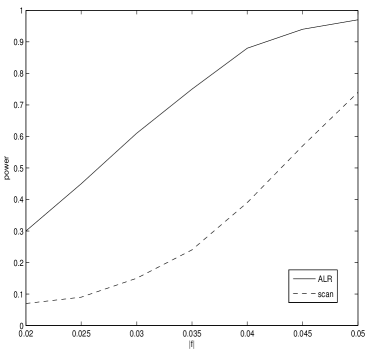
Figure 1: Left: Power of the scan and the ALR for detecting signals $f_{n}$ with fixed norm $\parallel\!\!f_{n}\!\!\parallel=0.04$ but varying spatial extent $|I_{n}|$, $n=10000$. Right: Power of the scan and the ALR for detecting signals $f_{n}$ with varying norms $\parallel\!\!f_{n}\!\!\parallel$ and random spatial extent. The power curves for the condensed ALR, the penalized scan, and the blocked scan are similar to those of the ALR and are not plotted, see Tables 1 and 2 for the numerical results.

Table 1 also shows an improvement in power of the condensed ALR vis-a-vis the ALR on small scales, illustrating Theorems 2 and  3. However, this improvement is modest, at least for the sample size under consideration, and thus the main advantage of the condensed scan is arguably the dramatic reduction in computation time to $O(n\log^{2}n)$ versus $O(n^{2})$ for the ALR. We were able to accurately simulate critical values for the condensed ALR with a sample size of 1 million in a matter of hours, whereas this computation would take hundreds of days for the ALR.

Table 2 shows how the power varies as function of $\parallel\!\!f_{n}\!\!\parallel$, see the right plot in Figure 1 for a visual representation. The spatial extent of the signal was chosen uniformly in $[0,1]$ in each of the 2000 Monte Carlo simulations. The power curves of the last four methods are again quite similar, and superior to that of the scan. One sees that the scan requires a signal with almost twice the norm to achieve the power of the four other methods. According to the results in the previous sections, this discrepancy increases with the sample size.

scale	0.01	0.05	0.1	0.15	0.2	0.25	0.3	0.35	0.4	0.45	0.5
scan	38	41	43	45	39	42	42	41	41	43	39
ALR	28	58	72	82	88	86	88	89	90	92	91
condensed ALR	36	61	72	80	87	85	87	88	90	91	91
penalized scan	37	61	72	80	85	84	85	86	87	90	89
blocked scan	41	59	69	77	82	80	82	82	84	87	86

Table 1: Power in percent for detecting signals $f_{n}$ with fixed norm $\parallel\!\!f_{n}\!\!\parallel=0.04$ but varying spatial extent $|I_{n}|$, $n=10000$.

$\parallel\!\!f_{n}\!\!\parallel\times 100$	2	2.5	3	3.5	4	4.5	5
scan	7	9	15	24	39	57	74
ALR	30	45	61	75	88	94	97
condensed ALR	30	44	60	75	87	94	97
penalized scan	26	40	57	74	85	93	97
blocked scan	24	35	51	69	82	92	96

Table 2: Power in percent for detecting signals $f_{n}$ with varying norms $\parallel\!\!f_{n}\!\!\parallel$ and random spatial extent, $n=10000$.

All power values in Tables 1 and 2 are with respect to a 5% significance level. The corresponding critical values were simulated with 10000 Monte Carlo samples, and the power was simulated with 2000 Monte Carlo samples. The location of the signal was chosen at random in each of these simulations to avoid confounding the results with the approximation scheme of the condensed ALR.

6 Conclusion

The scan is optimal only for detecting signals on the smallest scales. The ALR has a superior overall performance and is optimal for detecting signals on all scales except on the smallest ones, but the loss of power there appears to be modest. Moreover, by averaging the likelihood ratios over a particular subset of intervals rather than over all intervals, the resulting condensed ALR is simultaneously optimal for all scales and also allows for efficient computation. In contrast, improved versions of the scan, such as the penalized scan and the blocked scan, appear to require the use of scale-dependent critical values, and thus it appears that statistical optimality and computational efficiency have to be addressed separately for the scan.

The results of this paper are developed in the Gaussian white noise model since it is known that the conceptual results in that model are applicable and relevant for a wide range of related problems. We note that the concrete implementation of the results derived in the Gaussian white noise model requires additional work that depends on the concrete problem at hand. For example, in the univariate regression setting, Rohde (2008) employs local signed rank tests to transform non-Gaussian data into statistics with sub-gaussian tails, and Cai, Jeng, and Li (2011) employ a local median transformation for the same purpose. To see why such an additional step is required, note that the null distribution of both the scan and the ALR, as well as the form of the penalty term for the penalized scan, depend sensitively on the tails of the error distribution, and hence on the assumption of Gaussianity. The above papers show rigorously that the Gaussian white noise model is applicable after a local signed rank or a local median transformation, assuming only e.g. symmetry of the error distribution. These arguments are technically sophisticated and thus the transformation step constitutes a piece of methodological work by itself. It is thus helpful to separate the conceptual issues involving the scan and the ALR from the particular implementation and to present an unencumbered exposition in the Gaussian white noise model. In particular, the heuristics developed in this model give guidance how the corresponding problems might be addressed in related detection problems, such as the detection of clusters in models involving densities and intensities, as well as the important case of detecting multivariate signals. For example, in a regression type setting with irregularly spaced or multivariate data, the proportion of observations falling into the set $I$ would take the place of the size $|I|$ used above. Section 3 shows how to construct an approximating set that, on the one hand, results in computational efficiency and, on the other, provides the right ‘weighting’ of the various sizes of intervals in the condensed ALR to achieve statistical optimality. This idea can presumably be mimicked in a multivariate situation, where the construction would then depend on the entropy of the class of scanning windows. The implementation of this idea in the multivariate context is an interesting problem for future research. Another open problem is a theoretical result on the precision with which the scan and the ALR allow one to localize a signal once it is detected.

7 Proofs

Note that $f_{n}(x)=\mu_{n}{\bf 1}_{I_{n}}(x)$ implies for any interval $I\in{\cal J}_{n}$:

(4) $$\boldsymbol{Y}\!_{n}(I)\ =\ \boldsymbol{Z}_{n}(I)+sign(\mu_{n})\sqrt{n}|\mu_{n}|\frac{|I\cap I_{n}|}{\sqrt{|I|}}.$$

We use the following consequence of a result of Dümbgen and Spokoiny (2001).

Lemma 1

Let $\ell\in(0,1)$ and $J\in{\cal J}_{n}$, where $J$ does not depend on $\boldsymbol{Z}_{n}$. Then

$$\max_{I\in{\cal J}_{n}:I\subset J,|I|\geq\ell}|\boldsymbol{Z}_{n}(I)|\ \stackrel{{\scriptstyle d}}{{\leq}}\ L+\sqrt{2\log\frac{e|J|}{\ell}}$$

for a universal random variable $L$ which is finite almost surely.

Proof of Lemma 1: Writing $W$ for Brownian motion and $j,k$ for integer indices:

(5) $$\begin{split}\max_{\begin{subarray}{c}I\in{\cal J}_{n}:I\subset J\\ |I|\geq\ell\end{subarray}}\Bigl{(}|\boldsymbol{Z}_{n}(I)|-\sqrt{2\log\frac{e|J|}{|I|}}\Bigr{)}&\stackrel{{\scriptstyle d}}{{=}}\max_{\begin{subarray}{c}0\leq j<k\leq n|J|\\ k-j\geq n\ell\end{subarray}}\Bigl{(}\frac{|W(k)-W(j)|}{\sqrt{k-j}}-\sqrt{2\log\frac{e|J|n}{k-j}}\Bigr{)}\\ &\leq\sup_{\begin{subarray}{c}s,t\in{\boldsymbol{R}}:\\ 0\leq s<t\leq n|J|\end{subarray}}\Bigl{(}\frac{|W(t)-W(s)|}{\sqrt{t-s}}-\sqrt{2\log\frac{e|J|n}{t-s}}\Bigr{)}\\ &\stackrel{{\scriptstyle d}}{{=}}\sup_{0\leq s<t\leq 1}\Bigl{(}\frac{|W(t)-W(s)|}{\sqrt{t-s}}-\sqrt{2\log\frac{e}{t-s}}\Bigr{)}\ =:\ L\end{split}$$

by Brownian scaling. Thus the random variable $L$ defined above is universally applicable for all $n,\ell$, and $J$. Importantly, $L$ is finite almost surely, see Sec. 6.1 in Dümbgen and Spokoiny (2001). $\Box$

Proof of Theorem 1: As for part 1, (4) implies $M_{n}\ \geq\ |\boldsymbol{Y}\!_{n}(I_{n})|\ \geq\ -|\boldsymbol{Z}_{n}(I_{n})|+\sqrt{2\log n}+\epsilon_{n}\sqrt{\log n}$. Since $\boldsymbol{Z}_{n}(I_{n})\sim N(0,1)$ and $\epsilon_{n}\sqrt{\log n}\rightarrow\infty$, the claim follows from $\kappa_{n}=\sqrt{2\log n}+O(1)$, see (6).

For the proof of part 2, set $b_{n}:=\epsilon_{n}\sqrt{\log n}\rightarrow\infty$ and consider first the collection of intervals ${\cal J}_{n,1}:=\Bigl{\{}I\in{\cal J}_{n}:\ I\cap I_{n}\neq\emptyset$ and $|I_{n}|/b_{n}\leq|I|\leq b_{n}|I_{n}|\Bigr{\}}$. So $I\in{\cal J}_{n,1}$ implies $I\subset\Bigl{(}\frac{j_{n}-\lfloor b_{n}n|I_{n}|\rfloor}{n},\frac{k_{n}+\lfloor b_{n}n|I_{n}|\rfloor}{n}\Bigr{]}\cap(0,1]$ and thus Lemma 1 gives

$$\max_{I\in{\cal J}_{n,1}}|\boldsymbol{Z}_{n}(I)|\ \ \stackrel{{\scriptstyle d}}{{\leq}}\ \ L+\sqrt{2\log\frac{e(1+2b_{n})|I_{n}|}{|I_{n}|/b_{n}}}\ \ \leq\ \ L+2\sqrt{\log(3b_{n})}.$$

Together with (4) and $|I\cap I_{n}|\leq\sqrt{|I||I_{n}|}$, this yields

$$\begin{split}{\rm I\!P}_{f_{n}}\Bigl{(}\max_{I\in{\cal J}_{n,1}}|\boldsymbol{Y}\!_{n}(I)|>\kappa_{n}\Bigr{)}&\leq{\rm I\!P}\Bigl{(}\max_{I\in{\cal J}_{n,1}}|\boldsymbol{Z}_{n}(I)|+\sqrt{2\log n}-b_{n}>\kappa_{n}\Bigr{)}\\ &\leq{\rm I\!P}\Bigl{(}L>\kappa_{n}-\sqrt{2\log n}+b_{n}-2\sqrt{\log(3b_{n})}\Bigr{)}\\ &\rightarrow 0\ \ \ \mbox{ since }\kappa_{n}=\sqrt{2\log n}+O(1)\mbox{ by (\ref{kappa}).}\end{split}$$

Next, only if $b_{n}\leq\log^{3}\!n$ do we need to consider ${\cal J}_{n,2}:=\Bigl{\{}I\in{\cal J}_{n}:\ I\cap I_{n}\neq\emptyset$ and either $|I_{n}|/\log^{3}\!n\leq|I|\leq|I_{n}|/b_{n}\$ or $\ b_{n}|I_{n}|<|I|\leq|I_{n}|\log^{3}\!n\Bigr{\}}$. Similarly as above, $I\in{\cal J}_{n,2}$ implies that $I$ is contained in an interval $J\in{\cal J}_{n}$ with $|J|\leq(1+2\log^{3}\!n)|I_{n}|$. Thus Lemma 1 yields

$$\max_{I\in{\cal J}_{n,2}}|\boldsymbol{Z}_{n}(I)|\ \ \stackrel{{\scriptstyle d}}{{\leq}}\ \ L+\sqrt{2\log\frac{e(1+2\log^{3}\!n)|I_{n}|}{|I_{n}|/\log^{3}\!n}}\ \ \leq\ \ L+4\sqrt{\log\log n}.$$

One readily checks that $I\in{\cal J}_{n,2}$ implies $|I\cap I_{n}|\leq\sqrt{|I||I_{n}|/b_{n}}$. Thus (4) gives

$$\begin{split}{\rm I\!P}_{f_{n}}\Bigl{(}\max_{I\in{\cal J}_{n,2}}|\boldsymbol{Y}\!_{n}(I)|>\kappa_{n}\Bigr{)}&\leq{\rm I\!P}\Bigl{(}\max_{I\in{\cal J}_{n,2}}|\boldsymbol{Z}_{n}(I)|+\frac{\sqrt{2\log n}-b_{n}}{\sqrt{b_{n}}}>\kappa_{n}\Bigr{)}\\ &\leq{\rm I\!P}\Bigl{(}L>\kappa_{n}-\frac{\sqrt{2\log n}-b_{n}}{\sqrt{b_{n}}}-4\sqrt{\log\log n}\Bigr{)}\\ &\rightarrow 0\ \ \ \mbox{ since }\kappa_{n}=\sqrt{2\log n}+O(1).\end{split}$$

Finally, consider ${\cal J}_{n,3}:=\Bigl{\{}I\in{\cal J}_{n}:\ I\cap I_{n}=\emptyset\$ or $\ |I|\leq|I_{n}|/\log^{3}\!n\$ or $\ |I|>|I_{n}|\log^{3}\!n\Bigr{\}}$. Since $I\in{\cal J}_{n,3}$ implies $|I\cap I_{n}|\leq\sqrt{|I||I_{n}|/\log^{3}\!n}$, we get by (4),

$${\rm I\!P}_{f_{n}}\Bigl{(}\max_{I\in{\cal J}_{n,3}}|\boldsymbol{Y}\!_{n}(I)|>\kappa_{n}\Bigr{)}\ \leq\ {\rm I\!P}\Bigl{(}\max_{I\in{\cal J}_{n}}|\boldsymbol{Z}_{n}(I)|>\kappa_{n}-\frac{\sqrt{2\log n}-b_{n}}{\sqrt{\log^{3}\!n}}\Bigr{)}\ \rightarrow\ \alpha,$$

where the convergence follows from the following.

A sequence $\{c_{n}\}$ satisfies $\lim_{n}{\rm I\!P}\Bigl{(}\max_{I\in{\cal J}_{n}}|\boldsymbol{Z}_{n}(I)|>c_{n}\Bigr{)}=\alpha\$ if and only if

(6) $$c_{n}\ =\ \sqrt{2\log n}+(2\log n)^{-1/2}\Bigl{(}\frac{1}{2}\log\log n+C(\alpha)\Bigr{)}+o\Bigl{(}(\log n)^{-1/2}\Bigr{)}$$

for a certain constant $C(\alpha)$. This follows from Theorem 1.3 in Kabluchko (2008) or, with some work, from the earlier Theorem 1 in Siegmund and Venkatraman (1995).

Since ${\cal J}_{n}={\cal J}_{n,1}\cup{\cal J}_{n,2}\cup{\cal J}_{n,3}$ the theorem is proved. $\Box$

Proof of Theorem 2: We begin by showing that in the null case of no signal, $\boldsymbol{Y}\!_{n}=\boldsymbol{Z}_{n}$, we have

(7) $$A_{n}\ =\ O_{p}(1).$$

Note that $A_{n}$ is an average of correlated random variables that do not possess a finite first moment. In light of the converse to the strong law it is thus not at all obvious that (7) holds. For a proof let $m>0$ and define the event ${\cal B}_{m,n}:=\{|\boldsymbol{Z}_{n}((\frac{j}{n},\frac{k}{n}])|\leq C(\frac{k-j}{n})+m\mbox{ for all }0\leq j<k\leq n\}$, where $C(\delta):=\sqrt{2\log e/\delta}$. Then Markov’s inequality gives, for $\lambda>0$,

$$\begin{split}{\rm I\!P}_{0}(A_{n}>\lambda)&\leq\frac{1}{\lambda n^{2}}\sum_{j=0}^{n-1}\sum_{k=j+1}^{n}{\rm I\!E}\Bigl{[}\exp\Bigl{(}\frac{(\boldsymbol{Z}_{n}((\frac{j}{n},\frac{k}{n}]))^{2}}{2}\Bigr{)}\ 1({\cal B}_{m,n})\Bigr{]}\ +{\rm I\!P}({\cal B}_{m,n}^{c})\\ &\leq\frac{1}{\lambda n^{2}}\sum_{j=0}^{n-1}\sum_{k=j+1}^{n}\int_{-C(\frac{k-j}{n})-m}^{C(\frac{k-j}{n})+m}e^{z^{2}/2}\frac{1}{\sqrt{2\pi}}e^{-z^{2}/2}dz\ +{\rm I\!P}({\cal B}_{m,n}^{c})\\ &\leq\frac{1}{\lambda n^{2}}\sum_{j=0}^{n-1}\sum_{k=j+1}^{n}\Bigl{(}\sqrt{2\log\frac{en}{k-j}}+m\Bigr{)}+{\rm I\!P}({\cal B}_{m,n}^{c})\\ &\leq\frac{1}{\lambda}\Bigl{(}\frac{1}{n}\sum_{j=0}^{n-1}\int_{0}^{1}\sqrt{2\log e/u}\,du+m\Bigr{)}+{\rm I\!P}({\cal B}_{m,n}^{c})\\ &\leq\frac{4+m}{\lambda}+{\rm I\!P}(L>m)\end{split}$$

by (5). This sum can be made arbitrarily small by choosing $m$ and $\lambda$ appropriately, proving (7).

To prove parts 1 and 3 together we consider $f_{n}$ with arbitrary spatial extent and $|\mu_{n}|\sqrt{|I_{n}|}\geq\Bigl{(}\sqrt{4\log\frac{1}{|I_{n}|}}+b_{n}\Bigr{)}/\sqrt{n}$ with $b_{n}\rightarrow\infty$. Set $\epsilon_{n}:=\min\Bigl{(}1,b_{n}(\log\frac{e}{|I_{n}|})^{-1/2}\Bigr{)}$ and ${\cal J}(I_{n}):=\{I\in{\cal J}_{n}:I\subset I_{n}$ and $|I|\geq|I_{n}|(1-\epsilon_{n}/2)\}$. Then $\#{\cal J}(I_{n})\geq\lceil\epsilon_{n}n|I_{n}|/4\rceil^{2}$ since each of the $\lceil\epsilon_{n}n|I_{n}|/4\rceil$ smallest (largest) design points in $cl(I_{n})$ may serve as a left (right) endpoint for some $I\in{\cal J}(I_{n})$. Lemma 1 gives

$$\max_{I\in{\cal J}(I_{n})}|\boldsymbol{Z}_{n}(I)|\ \stackrel{{\scriptstyle d}}{{\leq}}\ L+\sqrt{2\log\frac{e}{1-\epsilon_{n}/2}}\ \leq\ L+2.$$

Together with $\frac{|I\cap I_{n}|}{\sqrt{|I||I_{n}|}}=\sqrt{\frac{|I|}{|I_{n}|}}\geq\sqrt{1-\frac{\epsilon_{n}}{2}}$ and (4) we get

$$\min_{I\in{\cal J}(I_{n})}|\boldsymbol{Y}\!_{n}(I)| \stackrel{{\scriptstyle d}}{{\geq}} \Bigl{(}\sqrt{4\log\frac{1}{|I_{n}|}}+b_{n}\Bigr{)}\sqrt{1-\frac{\epsilon_{n}}{2}}-L-2$$

$$\geq \sqrt{4\log\frac{1}{|I_{n}|}}+\frac{b_{n}}{9}-L-2,$$

since $(x+y)\sqrt{1-\min(1,y)/2}\geq x+\frac{y}{9}\$ for $x\in[0,2],y>0$. Thus, writing $R_{n}:=\frac{b_{n}}{9}-L-2$,

$$\begin{split}A_{n}&\geq\frac{\#{\cal J}(I_{n})}{n^{2}}\min_{I\in{\cal J}(I_{n})}\exp\Bigl{(}\frac{(\boldsymbol{Y}\!_{n}(I))^{2}}{2}\Bigr{)}\\ &\stackrel{{\scriptstyle d}}{{\geq}}\frac{\epsilon_{n}^{2}|I_{n}|^{2}}{4^{2}}\ \exp\Bigl{\{}2\log\frac{1}{|I_{n}|}+R_{n}\Bigl{(}R_{n}/2+\sqrt{4\log\frac{1}{|I_{n}|}}\Bigr{)}\Bigr{\}}\\ &=\frac{\epsilon_{n}^{2}}{4^{2}}\ \exp\Bigl{\{}R_{n}\Bigl{(}R_{n}/2+\sqrt{4\log\frac{1}{|I_{n}|}}\Bigr{)}\Bigr{\}}\\ &\geq\frac{\epsilon_{n}^{2}}{4^{2}}\Bigl{(}\log\frac{e}{|I_{n}|}\Bigr{)}\exp(R_{n}^{2}/2)\ 1(R_{n}\geq 1)\\ &\stackrel{{\scriptstyle a.s.}}{{\rightarrow}}\infty\ \ \ \mbox{ since }R_{n}\stackrel{{\scriptstyle a.s.}}{{\rightarrow}}\infty\ \mbox{ and }\epsilon_{n}\sqrt{\log\frac{e}{|I_{n}|}}\geq 1\mbox{ eventually.}\end{split}$$

The claim follows since $\tau_{n}=O(1)$ by (7).

For the proof of part 2 we partition ${\cal J}_{n}$ into ${\cal J}_{n,1}:=\{I\in{\cal J}_{n}:I\cap I_{n}\neq\emptyset$ and $|I_{n}|/\log^{4}\!\frac{1}{|I_{n}|}\leq|I|\leq|I_{n}|\log^{4}\!\frac{1}{|I_{n}|}\}$ and ${\cal J}_{n,2}:={\cal J}_{n}\cap{\cal J}_{n,1}^{c}$. We show for ${\cal J}={\cal J}_{n,1},{\cal J}_{n,2}$ that

(8) $$\frac{1}{n^{2}}\sum_{I\in{\cal J}}\Bigl{|}\exp\Bigl{(}\frac{(\boldsymbol{Y}\!_{n}(I))^{2}}{2}\Bigr{)}-\exp\Bigl{(}\frac{(\boldsymbol{Z}_{n}(I))^{2}}{2}\Bigr{)}\Bigr{|}\ \stackrel{{\scriptstyle P}}{{\rightarrow}}\ 0.$$

Since it can be shown that in the null case $f_{n}\equiv 0$, the ALR $A_{n}$ converges weakly to a continuous limit, the claim of part 2 follows from (8).

To prove (8) for ${\cal J}={\cal J}_{n,1}$ we follow the proof of part 2 of Theorem 1 (set $b_{n}:=\log^{4}\!\frac{1}{|I_{n}|}$ there) and conclude $\max_{I\in{\cal J}_{n,1}}|\boldsymbol{Z}_{n}(I)|\stackrel{{\scriptstyle d}}{{\leq}}L+2\sqrt{\log(3\log^{4}\!\frac{1}{|I_{n}|})}$. Hence for a fixed constant $\lambda$ which is specified below we obtain

$${\rm I\!P}\Bigl{(}{\cal A}_{n}\ :=\ \Bigl{\{}\max_{I\in{\cal J}_{n,1}}|\boldsymbol{Z}_{n}(I)|\leq\lambda\sqrt{\log\frac{1}{|I_{n}|}}\Bigr{\}}\Bigr{)}\ \rightarrow\ 1.$$

That proof also shows that every $I\in{\cal J}_{n,1}$ is contained in a certain interval of length $(1+2\log^{4}\!\frac{1}{|I_{n}|})|I_{n}|$, thus $\#{\cal J}_{n,1}\leq\Bigl{(}(1+2\log^{4}\!\frac{1}{|I_{n}|})n|I_{n}|\Bigr{)}^{2}$. On the event ${\cal A}_{n}$ we have, by (4),

$$\frac{1}{n^{2}}\sum_{I\in{\cal J}_{n,1}}\Bigl{|}\exp\Bigl{(}\frac{(\boldsymbol{Y}\!_{n}(I))^{2}}{2}\Bigr{)}-\exp\Bigl{(}\frac{(\boldsymbol{Z}_{n}(I))^{2}}{2}\Bigr{)}\Bigr{|}$$

$$\leq \frac{\#{\cal J}_{n,1}}{n^{2}}\ 2\ \exp\Bigl{(}\max_{I\in{\cal J}_{n,1}}\frac{(\boldsymbol{Z}_{n}(I))^{2}}{2}+\frac{n|\mu_{n}|^{2}|I_{n}|}{2}+\max_{I\in{\cal J}_{n,1}}|\boldsymbol{Z}_{n}(I)|\sqrt{n|I_{n}|}|\mu_{n}|\Bigr{)}$$

$$\leq 18\Bigl{(}\log\!\frac{1}{|I_{n}|}\Bigr{)}^{8}\ |I_{n}|^{2}\ \exp\Bigl{(}\frac{\lambda^{2}\log\frac{1}{|I_{n}|}}{2}+\frac{K^{2}}{2}\log\frac{1}{|I_{n}|}+\lambda K\log\frac{1}{|I_{n}|}\Bigr{)}$$

$$= 18\Bigl{(}\log\!\frac{1}{|I_{n}|}\Bigr{)}^{8}\ |I_{n}|^{2-\frac{K^{2}}{2}-\frac{\lambda^{2}}{2}-\lambda K}.$$

Since $\frac{K^{2}}{2}<2$ we can choose $\lambda=\lambda(K)>0$ such that the above expression goes to 0 as $|I_{n}|\rightarrow 0$, proving (8) for ${\cal J}={\cal J}_{n,1}$.

To prove (8) for ${\cal J}={\cal J}_{n,2}$, we proceed similarly as in the proof of (7) and employ the event ${\cal B}_{m,n}$ defined there. Then for $\lambda,m>0$, Markov’s inequality gives

$${\rm I\!P}_{f_{n}}\Bigl{(}\frac{1}{n^{2}}\sum_{I\in{\cal J}_{n,2}}\Bigl{|}\exp\Bigl{(}\frac{(\boldsymbol{Y}\!_{n}(I))^{2}}{2}\Bigr{)}-\exp\Bigl{(}\frac{(\boldsymbol{Z}_{n}(I))^{2}}{2}\Bigr{)}\Bigr{|}\ >\ \lambda\Bigr{)}$$

$$\leq \frac{1}{\lambda n^{2}}\sum_{I\in{\cal J}_{n,2}}{\rm I\!E}_{f_{n}}\Bigl{(}\Bigl{|}\exp\Bigl{(}\frac{(\boldsymbol{Y}\!_{n}(I))^{2}}{2}\Bigr{)}-\exp\Bigl{(}\frac{(\boldsymbol{Z}_{n}(I))^{2}}{2}\Bigr{)}\Bigr{|}1({\cal B}_{m,n})\Bigr{)}+{\rm I\!P}({\cal B}_{m,n}^{c}).$$

Since (5) gives ${\rm I\!P}({\cal B}_{m,n}^{c})\leq{\rm I\!P}(L>m)\rightarrow 0$ as $m\rightarrow\infty$, it is enough to show that for any fixed $m$ the above expectation converges to 0 as $n\rightarrow\infty$, uniformly in $I\in{\cal J}_{n,2}$. Using $\boldsymbol{Z}_{n}(I)\sim$ N(0,1) and writing $\delta_{I}:=\sqrt{n}|\mu_{n}|\frac{|I\cap I_{n}|}{\sqrt{|I|}}$ and $C(|I|):=\sqrt{2\log e/|I|}$, we get with (4),

(9) $${\rm I\!E}_{f_{n}}\Bigl{(}\Bigl{|}\exp\Bigl{(}\frac{(\boldsymbol{Y}\!_{n}(I))^{2}}{2}\Bigr{)}-\exp\Bigl{(}\frac{(\boldsymbol{Z}_{n}(I))^{2}}{2}\Bigr{)}\Bigr{|}1({\cal B}_{m,n})\Bigr{)}$$

$$\leq \frac{1}{\sqrt{2\pi}}\int_{-C(|I|)-m}^{C(|I|)+m}\Bigl{|}\exp(z\delta_{I}+\delta_{I}^{2}/2)-1\Bigr{|}dz$$

$$\leq \sqrt{\frac{2}{\pi}}\exp\Bigl{(}\delta_{I}(C(|I|)+m)+\delta_{I}^{2}/2\Bigr{)}\Bigl{(}\delta_{I}(C(|I|)+m)^{2}+\delta_{I}^{2}(C(|I|)+m)/2\Bigl{)}$$

by bounding the function $z\mapsto\exp(z\delta+\delta^{2}/2)-1$ above and below by the Mean Value Theorem. Next we show that, as $n\rightarrow\infty$,

(10) $$\delta_{I}\rightarrow 0\ \ \ \mbox{ and }\ \ \ \delta_{I}C^{2}(|I|)\rightarrow 0\ \ \ \mbox{ uniformly in }I\in{\cal J}_{n,2}.$$

This conclusion then also holds for the expression in (9), and (8) follows.

To prove (10), note that $\delta_{I}=K\sqrt{\log\frac{1}{|I_{n}|}}\ \frac{|I\cap I_{n}|}{\sqrt{|I||I_{n}|}}$. If $I\cap I_{n}=\emptyset$, then $\delta_{I}=0$. If $|I|<|I_{n}|/\log^{4}\!\frac{1}{|I_{n}|}$, then the bound $|I\cap I_{n}|\leq|I|$ yields $\delta_{I}\leq K(\log\frac{1}{|I_{n}|})^{-3/2}$, while the monotonicity of the function $x\mapsto\sqrt{x}\log e/x$ for $x\in(0,e^{-1})$ gives

$$\delta_{I}C^{2}(|I|) \leq 2K\sqrt{\log\frac{1}{|I_{n}|}}\sqrt{\frac{|I|}{|I_{n}|}}\log\frac{e}{|I|}$$

$$\leq 2K\Bigl{(}\log\frac{1}{|I_{n}|}\Bigr{)}^{-3/2}\log\frac{e\log^{4}\!\frac{1}{|I_{n}|}}{|I_{n}|}$$

$$\leq 6K\Bigl{(}\log\frac{1}{|I_{n}|}\Bigr{)}^{-1/2}$$

if $n$ is large enough so that $|I_{n}|/\log^{4}\!\frac{1}{|I_{n}|}\leq e^{-1}$.

If $|I|>|I_{n}|\log^{4}\!\frac{1}{|I_{n}|}$, then the bound $|I\cap I_{n}|\leq|I_{n}|$ yields again $\delta_{I}\leq K(\log\frac{1}{|I_{n}|})^{-3/2}$, while $\delta_{I}C^{2}(|I|)\leq 2K(\log\frac{1}{|I_{n}|})^{-3/2}\log\frac{e}{|I|}\leq 2K(\log\frac{1}{|I_{n}|})^{-1/2}$. $\Box$

Proof of Theorem 3: Before proceeding to the proof, we sketch an explanation for the choice of the grid spacing $d_{\ell}$. For given $I_{n}$, let $\ell$ be such that the intervals in $\boldsymbol{{\cal I}}_{app}(\ell)$ have length about $|I_{n}|$. Thus $m_{\ell}\sim n|I_{n}|$, i.e. $\ell\approx\log_{2}\frac{e}{|I_{n}|}$. An interval $I$ results in a significant likelihood ratio provided its endpoints lie in a $\frac{\epsilon_{n}}{2}|I_{n}|$ neighborhood of the endpoints of $I_{n}$, where $\epsilon_{n}:=\min\Bigl{(}1,b_{n}(\log\frac{e}{|I_{n}|})^{-1/2}\Bigr{)}$. Thus the number of significant intervals in $\boldsymbol{{\cal I}}_{app}(\ell)$ is $\sim(\epsilon_{n}|I_{n}|n/d_{\ell})^{2}$. Under (1) the size of the corresponding likelihood ratios is $\gg\frac{(\log_{2}\frac{e}{|I_{n}|})^{p}}{|I_{n}|}$ for arbitrary $p>0$. Thus optimality of $A_{n,cond}$ obtains if the number of significant intervals in $\boldsymbol{{\cal I}}_{app}(\ell)$ is at least $\#\boldsymbol{{\cal I}}_{app}\frac{|I_{n}|}{(\log_{2}\frac{e}{|I_{n}|})^{p}}$ for some fixed $p>0$, and even if the number is smaller by some factor $\epsilon_{n}^{k}$, since $\epsilon_{n}\sqrt{\log_{2}\frac{e}{|I_{n}|}}\geq 1$. Solving this inequality for $d_{\ell}$ yields $d_{\ell}\leq\sqrt{\frac{n^{2}|I_{n}|\ell^{p}}{\#\boldsymbol{{\cal I}}_{app}}}$. Requiring $\#\boldsymbol{{\cal I}}_{app}\sim n(\log n)^{q}$ for some $q>0$ for computational efficiency suggests the choice $d_{\ell}\sim\sqrt{m_{\ell}\ell^{p}(\log n)^{-q}}$. Computing $\#\boldsymbol{{\cal I}}_{app}$ shows that this choice of $d_{\ell}$ is indeed consistent with $\#\boldsymbol{{\cal I}}_{app}\sim n(\log n)^{q}$ provided $p>1$. Further, it will be seen that $A_{n,cond}=O_{p}(1)$ under the null hypothesis requires $\sum_{\ell}\ell^{1/2-p}<\infty$, i.e. $p>3/2$. Finally, optimal detection for very small intervals $I_{n}$ requires that their endpoints are approximated exactly, i.e. it is necessary to have $d_{\ell}=1$ for large $\ell$. Thus we need an appropriate combination of a small $p>3/2$ and a large $q$. Since the required large $q$ results in a noticeably worse computation time, we prefer to stick to a $O(n\log^{2}n)$ algorithm by setting $p=8/5$, $q=2$, and by explicitly considering all small intervals containing up to $\log n$ design points in lieu of choosing a larger $q$.

We now prove the theorem, starting with the claim about the computational complexity. Since $\boldsymbol{{\cal I}}_{app}(\ell)$ allows only every $d_{\ell}$th design point as a potential endpoint for an interval, there are at most $\lceil n/d_{\ell}\rceil$ left endpoints. For each left endpoint there are at most $\lceil 2m_{\ell}/d_{\ell}\rceil$ right endpoints since each interval contains not more than $2m_{\ell}$ design points. Thus

(11) $$\#\boldsymbol{{\cal I}}_{app}(\ell)\ \leq\ \Bigl{\lceil}\frac{n}{d_{\ell}}\Bigr{\rceil}\Bigl{\lceil}\frac{2m_{\ell}}{d_{\ell}}\Bigr{\rceil}\ \leq\ 3\frac{n\log^{2}\!n}{\ell^{8/5}}\ \ \ \mbox{ and}$$

(12) $$\#\boldsymbol{{\cal I}}_{small}\ \leq\ n\log n\ \ \ \ \mbox{ since }m_{\ell_{max}}\leq\log n.\mbox{ Hence}$$

(13) $$\#\boldsymbol{{\cal I}}_{app}\ \leq\ \sum_{\ell=1}^{\ell_{max}}3\frac{n\log^{2}\!n}{\ell^{8/5}}+n\log n\ \leq\ 9n\log^{2}\!n.$$

$\exp\Bigl{(}\frac{(\boldsymbol{Y}\!_{n}(I))^{2}}{2}\Bigr{)}$ can be evaluated in a constant number of steps after an initial one-time computation of the cumulative sum vector of $(Y_{i},1\leq i\leq n)$. Since that computation has complexity $O(n)$, the overall computational complexity of computing $A_{n,cond}$ is dominated by the cardinality of $\boldsymbol{{\cal I}}_{app}$ and hence is $O(n\log^{2}\!n)$.

Next we show that for $f_{n}\equiv 0$:

(14) $$A_{n,cond}\ =\ O_{p}(1)\ \ \mbox{ as }n\rightarrow\infty.$$

Proceeding as in the proof of (7) it is enough to show that

(15) $$\frac{1}{\#\boldsymbol{{\cal I}}_{app}}\sum_{I\in\boldsymbol{{\cal I}}_{app}}\sqrt{2\log\frac{1}{|I|}}\ =\ O(1).$$

Since $I\in\boldsymbol{{\cal I}}_{app}(\ell)$ implies $|I|>\frac{m_{\ell}}{n}=2^{-\ell}$, we obtain with (11) and (12),

$$\sum_{I\in\boldsymbol{{\cal I}}_{app}}\sqrt{2\log\frac{1}{|I|}} \leq \sum_{\ell=1}^{\ell_{max}}\#\boldsymbol{{\cal I}}_{app}(\ell)\sqrt{2\ell}\ +n(\log n)\sqrt{2\log n}$$

$$\leq 5n\log^{2}\!n\sum_{\ell=1}^{\infty}\frac{\ell^{1/2}}{\ell^{8/5}}\ +n(\log n)^{2}$$

$$\leq 56n\log^{2}\!n.$$

On the other hand, $\#\boldsymbol{{\cal I}}_{app}\geq\#\boldsymbol{{\cal I}}_{app}(2)\geq\frac{1}{10}n(\log n)^{2}$ by considerations similar to those establishing (11). (15) follows.

To establish optimality of $A_{n,cond}$, we proceed as in the proof of Theorem 2 and consider $f_{n}$ with arbitrary spatial extent and $|\mu_{n}|\sqrt{|I_{n}|}\geq\Bigl{(}\sqrt{2\log\frac{1}{|I_{n}|}}+b_{n}\Bigr{)}/\sqrt{n}$, where $b_{n}\rightarrow\infty$. As before we define $\epsilon_{n}:=\min\Bigl{(}1,b_{n}(\log\frac{e}{|I_{n}|})^{-1/2}\Bigr{)}$ and ${\cal J}(I_{n}):=\{I\in{\cal J}_{n}:I\subset I_{n}$ and $|I|\geq|I_{n}|(1-\epsilon_{n}/2)\}$. Intervals $I\in{\cal J}(I_{n})$ contribute significant LR statistics to $A_{n,cond}$. Since we now require that the endpoints of these intervals fall on a $d_{\ell}$- grid, there are now many fewer of these intervals. But this is more than compensated by the small cardinality of $\boldsymbol{{\cal I}}_{app}$ appearing in the divisor of $A_{n,cond}$. This fact allows us to detect $f_{n}$ with a norm that is smaller than in Theorem 2. In more detail, take the integer $\ell$ so $m_{\ell}<n|I_{n}|(1-\epsilon_{n}/4)\leq 2m_{\ell}$.

Lemma 2

$$\mbox{If }\ell \leq \ell_{max},\mbox{ then }\frac{\#\Bigl{(}{\cal J}(I_{n})\cap\boldsymbol{{\cal I}}_{app}(\ell)\Bigr{)}}{\#\boldsymbol{{\cal I}}_{app}}\geq\frac{\epsilon_{n}^{2}|I_{n}|}{9^{3}\Bigl{(}\log_{2}\frac{e}{|I_{n}|}\Bigr{)}^{8/5}}.$$

$$\mbox{If }\ell > \ell_{max},\mbox{ then }\frac{\#\Bigl{(}{\cal J}(I_{n})\cap\boldsymbol{{\cal I}}_{small}\Bigr{)}}{\#\boldsymbol{{\cal I}}_{app}}\geq\frac{\epsilon_{n}^{2}|I_{n}|}{32^{2}\Bigl{(}\log_{2}\frac{e}{|I_{n}|}\Bigr{)}^{2}}.$$

As in the proof of Theorem 2 we find $\min_{I\in{\cal J}(I_{n})}|\boldsymbol{Y}\!_{n}(I)|\stackrel{{\scriptstyle d}}{{\geq}}\sqrt{2\log\frac{1}{|I_{n}|}}+R_{n}$, where $R_{n}:=\frac{b_{n}}{9}-L-2$. Thus in the case $\ell\leq\ell_{max}$, Lemma 2 gives

$$\begin{split}A_{n,cond}&\geq\frac{\#\Bigl{(}{\cal J}(I_{n})\cap\boldsymbol{{\cal I}}_{app}(\ell)\Bigr{)}}{\#\boldsymbol{{\cal I}}_{app}}\min_{I\in{\cal J}(I_{n})}\exp\Bigl{(}\frac{(\boldsymbol{Y}\!_{n}(I))^{2}}{2}\Bigr{)}\\ &\stackrel{{\scriptstyle d}}{{\geq}}\frac{\epsilon_{n}^{2}|I_{n}|}{9^{3}\Bigl{(}\log_{2}\frac{e}{|I_{n}|}\Bigr{)}^{8/5}}\ \exp\Bigl{\{}\log\frac{1}{|I_{n}|}+R_{n}\Bigl{(}R_{n}/2+\sqrt{2\log\frac{1}{|I_{n}|}}\Bigr{)}\Bigr{\}}\\ &=\frac{\epsilon_{n}^{2}}{9^{3}\Bigl{(}\log_{2}\frac{e}{|I_{n}|}\Bigr{)}^{8/5}}\ \exp\Bigl{\{}R_{n}\Bigl{(}R_{n}/2+\sqrt{2\log\frac{1}{|I_{n}|}}\Bigr{)}\Bigr{\}}\\ &\geq C\epsilon_{n}^{2}\Bigl{(}\log\frac{e}{|I_{n}|}\Bigr{)}\exp(R_{n}^{2}/2)\ 1(R_{n}\geq 1)\ \mbox{ for some universal }C>0\\ &\stackrel{{\scriptstyle a.s.}}{{\rightarrow}}\infty\ \ \ \mbox{ since }R_{n}\stackrel{{\scriptstyle a.s.}}{{\rightarrow}}\infty\ \mbox{ and }\epsilon_{n}\sqrt{\log\frac{e}{|I_{n}|}}\geq 1\mbox{ eventually.}\end{split}$$

In the case $\ell>\ell_{max}$, the same conclusion obtains by using $\boldsymbol{{\cal I}}_{small}$ in place of $\boldsymbol{{\cal I}}_{app}(\ell)$. The claim then follows since the critical value of $A_{n,cond}$ stays bounded, by (14).

Thus the crucial difference with Theorem 2 is the stronger inequality provided by Lemma 2. The corresponding inequality for Theorem 2 is $\#{\cal J}(I_{n})/n^{2}\geq\epsilon_{n}^{2}|I_{n}|^{2}/4^{2}$, and the extra term $|I_{n}|$ causes the loss of efficiency in the case when the spatial extent $|I_{n}|$ is small.

It remains to prove Lemma 2. Elementary considerations show that one can find sets ${\cal I}_{n,left}$ and ${\cal I}_{n,right}$, each consisting of $p:=\lceil\epsilon_{n}n|I_{n}|/8\rceil$ consecutive integers, such that $(j,k)\in{\cal I}_{n,left}\times{\cal I}_{n,right}$ implies $(\frac{j}{n},\frac{k}{n}]\in{\cal J}(I_{n})$, and also $m_{\ell}<k-j\leq 2m_{\ell}$ if $\ell\leq\ell_{max}$, resp. $k-j\leq m_{\ell_{max}}$ if $\ell>\ell_{max}$. Thus, in the latter case, we immediately obtain $\#\Bigl{(}{\cal J}(I_{n})\cap\boldsymbol{{\cal I}}_{small}\Bigr{)}\geq p^{2}$, and the claim of the Lemma obtains with (13), $n|I_{n}|\geq 1$, and $\log n\leq\frac{4}{3}\log_{2}\frac{e}{|I_{n}|}$, which follows from $\ell>\ell_{max}$. In the case $\ell\leq\ell_{max}$, only a subset of the $p^{2}$ intervals $\Bigl{\{}(\frac{j}{n},\frac{k}{n}]$: $(j,k)\in{\cal I}_{n,left}\times{\cal I}_{n,right}\Bigr{\}}$ belongs to ${\cal J}(I_{n})\cap\boldsymbol{{\cal I}}_{app}(\ell)$, namely those for which both $j$ and $k$ lie on the $d_{\ell}$-grid. The number of such indices $j$ is at least $\lfloor\frac{p}{d_{\ell}}\rfloor\geq\lceil\frac{\epsilon_{n}\sqrt{n|I_{n}|}\log n}{9\ \ell^{4/5}}\rceil$ for $n$ large enough, where this inequality follows from the fact that $\ell\leq\ell_{max}$ implies $n|I_{n}|>m_{\ell}\geq(\log n)/2$ and $d_{\ell}\geq(\log n)^{3/10}$; further, $\epsilon_{n}\sqrt{\log n}\rightarrow\infty$ by the definition of $\epsilon_{n}$. The same bound obtains for the number of indices $k$ that lie on the $d_{\ell}$-grid. The claim of the Lemma then follows with (13) and $\ell\leq\log_{2}\frac{e}{|I_{n}|}$, which is a consequence of the definition of $\ell$. $\Box$

References

Arias-Castro, E., Donoho, D.L., and Huo, X. (2005). Near-optimal detection of geometric objects by fast multiscale methods.  IEEE Trans. Inform. Th. 51, 2402–2425.

Burnashev, M.V. and Begmatov, I.A. (1990). On a problem of detecting a signal that leads to stable distributions. Theory Probab. Appl. 35, 556–560.

Cai, T., Jeng, X.J., and Li, H. (2011). Robust detection and identification of sparse segments in ultra-high dimensional data analysis. Manuscript.

Chan, H.P. (2009). Detection of spatial clustering with average likelihood ratio test statistics.  Ann. Statist. 37, 3985–4010.

Chan, H.P. and Walther, G. (2011). Detection with the scan and the average likelihood ratio.  Manuscript. January 2011.

Chan, H.P. and Zhang, N.R. (2009). Local average likelihood ratio test statistics with applications in genomics and change-point detection.  Manuscript.

Dümbgen, L. (1998). New goodness-of-fit tests and their application to nonparametric confidence sets. Ann. Statist. 26, 288–314.

Dümbgen, L. and Spokoiny, V.G. (2001). Multiscale testing of qualitative hypotheses.  Ann. Statist. 29, 124–152.

Dümbgen, L. and Walther, G. (2008). Multiscale inference about a density.  Ann. Statist. 36, 1758–1785.

Gangnon, R.E. and Clayton, M.K. (2001). The weighted average likelihood ratio test for spatial disease clustering. Statistics in Medicine 20, 2977–2987.

Glaz, J. and Balakrishnan, N. (ed.) (1999). Scan statistics and Applications.  Birkhäuser, Boston

Glaz, J., Naus, J., and Wallenstein, S. (2001). Scan Statistics.  Springer, New York

Glaz, J., Poznyakov, V., and Wallenstein, S. (ed.) (2009). Scan Statistics: Methods and Applications.  Birkhauser, Boston

Kabluchko, Z. (2008). Extreme-value analysis of standardized Gaussian increments. Manuscript.

Kulldorff, M. (1997). A spatial scan statistic.  Commun. Statist. - Theory Meth. 26, 1481–1496.

Lepski, O.V. and Tsybakov, A.B. (2000). Asymptotically exact nonparametric hypothesis testing in sup-norm and at a fixed point.  Probab. Theory Related Fields 117, 17–48.

Neill, D. and Moore, A. (2004). A fast multi-resolution method for detection of significant spatial disease clusters. Adv. Neur. Info. Proc. Sys. 10, 651–658.

Neill, D. (2009). An empirical comparison of spatial scan statistics for outbreak detection. Internat. Journal of Health Geographics 8, 1–16.

Rohde, A. (2008). Adaptive goodness-of-fit tests based on signed ranks. Ann. Statist. 36, 1346–1374.

Rufibach, K. and Walther, G. (2010). The block criterion for multiscale inference about a density, with applications to other multiscale problems.  Journal of Computational and Graphical Statistics 19, 175–190.

Shiryaev, A.N. (1963). On optimum methods in quickest detection problems.  Theory Probab. Appl. 8, 22-46.

Siegmund, D. and Venkatraman, E.S. (1995). Using the generalized likelihood ratio statistic for sequential detection of a change-point.  Ann. Statist. 23, 255–271.

Siegmund, D. (2001). Is peak height sufficient? Genetic Epidemiology 20, 403–408.

Walther, G. (2010). Optimal and fast detection of spatial clusters with scan statistics.  Ann. Statist. 38, 1010-1033.