Prediction of the derivative discontinuity in density functional theory from an electrostatic description of the exchange and correlation potential

Abstract

We propose a new approach to approximate the exchange and correlation (XC) functional in density functional theory. The XC potential is considered as an electrostatic potential, generated by a fictitious XC density, which is in turn a functional of the electronic density. We apply the approach to develop a correction scheme that fixes the asymptotic behavior of any approximated XC potential for finite systems. Additionally, the correction procedure gives the value of the derivative discontinuity; therefore it can directly predict the fundamental gap as a ground-state property.

An important and long standing topic in density functional theory (DFT) Hoh1964PR ; *Koh1965PR is the prediction of the fundamental gap Coh2009Sci ; *Per1985IJQC; Gru2006JCP $E_{\mathrm{g}}$, which is defined as the difference of the ionization energy and the electron affinity. In DFT, the gap is not simply the difference between the Kohn-Sham (KS) eigenvalues of the highest occupied molecular orbital (HOMO) and the lowest unoccupied molecular orbital (LUMO). Instead, it is given by Per1982PRL ; *Per1983PRL; *Sha1983PRL

$$E_{\mathrm{g}}=\epsilon_{\mathrm{LUMO}}-\epsilon_{\mathrm{HOMO}}+\Delta_{\mathrm{xc}}\ ,$$ (1)

where $\epsilon_{\mathrm{HOMO}}$ and $\epsilon_{\mathrm{LUMO}}$ are the HOMO and LUMO KS eigenvalues, respectively, and $\Delta_{\mathrm{xc}}$ is the derivative discontinuity (DD) of the XC energy with respect to the particle number N,

$$\Delta_{\mathrm{xc}}=V_{\mathrm{xc}}(N^{+})-V_{\mathrm{xc}}(N^{-})\ .$$ (2)

For the local density approximation (LDA) and many generalized gradient approximations (GGA), the DD is zero Toz2003MP . In these approximations the predicted gap is effectively the KS gap, which severely underestimates the experimental value. Even for functionals that are discontinuous with the particle number, the DD is not simple to calculate Cha1999JCP ; All2002MP ; Gru2006JCP ; Hel2007EPL ; *Hel2009PRA; *Lat2010ZPC. Alternatively, XC approximations have been proposed where the KS gap is directly used to predict the gap Zhe2011PRL ; *Mar2011PRB; *Dea2010PRB; *Tra2009PRL; *Son2007JCP; *Hey2003JCP; *Tou2004PRA avoiding the calculation of the DD.

In this article, we present an XC functional for finite systems that, with similar computational cost as a LDA or GGA calculation, has the right asymptotic limit for low density regions and directly provides the value of the DD. Hence, the proposed functional can predict the fundamental gap for an atom or molecule as a ground state property.

The approach that we advocate is not based on increasing the number of functional variables, but on changing the way that the XC potential is described: we consider the XC potential as an electrostatic potential, generated by a fictitious XC charge density. In contrast to directly modelling the potential, the XC density becomes the quantity to approximate as a functional of the electronic density $n$.

Given a XC potential $V_{\mathrm{xc}}$, we define the XC density $n_{\mathrm{xc}}$ by the Poisson equation (atomic units are used throughout)

$$\nabla^{2}V_{\mathrm{xc}}({\bm{r}})=-4\pi\,n_{\mathrm{xc}}({\bm{r}})\ ,$$ (3)

with the boundary condition $V_{\mathrm{xc}}({\bm{r}}\to\infty)=0$.

The justification for this approach comes from an important property of the XC potential: the so-called asymptotic limit Alm1985PRB ; Van1994PRA ,

$$V_{\mathrm{xc}}({\bm{r}})\approx-\frac{1}{\left|{\bm{r}}\right|}\quad(\left|{\bm{r}}\right|\to\infty)\ ,$$ (4)

The LDA and most GGAs do not obey the asymptotic limit condition. In part, this common deficiency can be explained simply. In regions that are spatially far away from the system, the density and its derivatives decay exponentially to zero Van1994PRA . It is difficult to use local values of the density and its derivatives to reproduce a field that decays to zero much more slowly.

For the XC density the asymptotic limit implies two simple conditions: normalization and localization. Formally,

$$n_{\mathrm{xc}}({\bm{r}}) =0\quad(\left|{\bm{r}}\right|\to\infty)\ ,$$ (5a)

$$\int\mathrm{d}{\bm{r}}\,n_{\mathrm{xc}}({\bm{r}}) =-1\ ,$$ (5b)

(proof in supp. mat. suppmat ). These constraints are similar to the ones for the electronic density. So, in principle, it is simple to construct a local or semi-local density functional $n_{\mathrm{xc}}[n]$ with the proper asymptotic limit. In fact, a direct example of this XC density based approach is the functional $n_{\mathrm{xc}}[n]({\bm{r}})=-n({\bm{r}})/N$, which yields the Fermi-Amaldi XC potential Fer1934ACI ; *Par1995PRA and provides an accurate approximation of $V_{\mathrm{xc}}$ in the asymptotic regime Zha1994PRA ; Ume2006PRA .

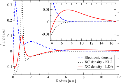
Figure 1: KLI electronic density and KLI and LDA XC densities for the beryllium atom. The inset details the asymptotic region, where the KLI XC density shows the correct behavior. The LDA XC density is incorrect in this region, with a positive part that screens the charge in the central region.

It is illustrative to see what the XC density looks like for standard DFT functionals. For a given XC potential, $n_{\mathrm{xc}}$ can be calculated analytically (see supp. mat. suppmat ), but in practice it is simpler to evaluate Eq. (3) numerically. In Fig. 1, we compare $n_{\mathrm{xc}}$ for LDA and exact exchange in the Krieger-Li-Iafrate (KLI) Kri1992PRA approximation. As can be seen from the figure, for large radius the KLI XC density correctly goes to zero faster than the electronic density. On the other hand, the LDA XC density becomes positive. This positive XC charge screens the XC charge in the central region making the total XC charge zero and therefore causing the potential to decay exponentially.

As a first application of our approach, we propose a correction method to enforce the proper asymptotic limit for functionals that do not have it by construction. Given a certain potential $\bar{V}_{\mathrm{xc}}$, we calculate the associated $\bar{n}_{\mathrm{xc}}$ from Eq. (3). To this XC density we apply the correction procedure, that generates a corrected XC density $n^{c}_{\mathrm{xc}}$. In turn, the corrected XC density is used to reconstruct the corrected XC potential $V^{c}_{\mathrm{xc}}$ by solving Eq. (3).

The correction procedure for $\bar{n}_{\mathrm{xc}}$ enforces it to be localized by setting it to zero when the local value of electronic density is below a certain threshold $\eta$. This simple procedure can be written as a correction term $\Delta n_{\mathrm{xc}}$ to be added to the XC density of the original functional,

$$\Delta n_{\mathrm{xc}}[n]({\bm{r}},\eta)=\ \left\{\begin{array}[]{ll}0&\mbox{if }n({\bm{r}})\geq\eta\\ -\bar{n}_{\mathrm{xc}}[n]({\bm{r}})&\mbox{if }n({\bm{r}})<\eta\end{array}\right.\ .$$ (6)

To determine the parameter $\eta$, for each density we obtain an optimized value $\eta_{0}$ that tries to enforce Eq. (5b). First, we define the total XC charge as a function of $\eta$

$$q_{\mathrm{xc}}(\eta)=\int\mathrm{d}{\bm{r}}\,\left\{\bar{n}_{\mathrm{xc}}[n]({\bm{r}})+\Delta n_{\mathrm{xc}}[n]({\bm{r}},\eta)\right\}\ .$$ (7)

Ideally, from Eq. (5b), we need to find $\eta_{0}$ such that $q_{\mathrm{xc}}(\eta_{0})=-1$. However, there is no guarantee about the existence or uniqueness of $\eta_{0}$. So we choose $\eta_{0}$ such that $q_{\mathrm{xc}}(\eta_{0})$ has the closest value to -1, with $\eta_{0}$ restricted to be smaller than the first minimum of $q_{\mathrm{xc}}(\eta)$. (See supp. mat. suppmat .)

When $q_{\mathrm{xc}}(\eta_{0})\neq-1$, Eq. (5b) is still not satisfied, so we rescale the correction by $\left|q_{\mathrm{xc}}(\eta_{0})\right|^{-1}$. The final expression for the XC density of the corrected functional is

$$n^{c}_{\mathrm{xc}}({\bm{r}})=\bar{n}_{\mathrm{xc}}({\bm{r}})+\frac{1}{\left|q_{\mathrm{xc}}(\eta_{0})\right|}\Delta n_{\mathrm{xc}}({\bm{r}},\eta_{0})\ .$$ (8)

This rescaling form guarantees that Eq. (5b) is satisfied, and that the original XC potential is changed as little as possible in the central region (the region where $n\geq\eta_{0}$).

In theory, it is only the exchange term that is responsible for the long range behavior, due to the much faster decay of the correlation term Van1994PRA , therefore, the correction can be applied either to the exchange potential or the full XC potential. In this work, we apply it to the exchange part of the LDA functional, and we call the combination of the corrected LDA exchange and LDA correlation (in the Perdew-Wang form Per1992PRBb ) the corrected exchange density LDA (CXD-LDA). For spin-polarized systems, the correction is calculated for the spin-unpolarized potential using the total density. Then the difference between the corrected potential and the original one is added to the XC potential for each spin component.

To test the CXD-LDA functional, we performed calculations for atoms, hydrogen to strontium, and for a set of small molecules. We implemented the correction procedure in the APE Oli2008CPC and Octopus Cas2006PSSB codes. We find that the optimized value of $\eta_{o}$ changes significantly for different systems. For most atoms $q_{\mathrm{xc}}(\eta_{0})\neq-1$ while for all the tested molecules $q_{\mathrm{xc}}(\eta_{0})=-1$ (see supp. mat. suppmat ). The numerical cost of a self-consistent solution using the correction is similar to the LDA calculation (see supp. mat. for details suppmat ).

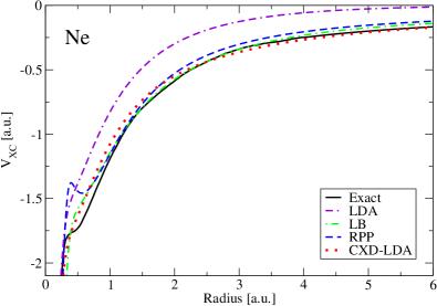
Figure 2: CXD-LDA potential for neon. Comparison with the LDA, LB Van1994PRA , RPP Ras2010JCP and the exact Zha1994PRA potentials.

In Fig. 2, we show the CXD-LDA potential for Ne compared with an accurate approximation to the exact potential Zha1994PRA , the original LDA functional and two functionals that have the correct asymptotic behavior: the van Leeuwen-Baerends (LB) GGA Van1994PRA and the Räsänen-Pittalis-Proetto (RPP) meta-GGA Ras2010JCP .

For atoms it is simple to understand the effect of the correction procedure. Due to the spherical symmetry and the monotonically-decreasing density, the correction XC charge $\Delta n_{\mathrm{xc}}$ is a spherical shell. By Newton’s shell theorem, the correction potential will be constant in the central region. Outside, the correction will decay close to $-1/r$. We can expect this behavior to be similar for more complex systems if the $n({\bm{r}})=\eta_{0}$ surface is close to a sphere (see supp. mat. suppmat ).

The shape of the correction is similar to the one proposed by Casida and Salahub Cas1998IJQC ; Cas2000JCP , who argument that a shift of the XC potential in the central region is necessary to fix the asymptotic limit of the LDA potential. Moreover, they show that the shift is related to the DD of the energy with respect to the particle number. As in our method the shift appears naturally from imposing the asymptotic limit, we can obtain the value of the DD.

To obtain the relation between the DD and the shift, we assume that a potential $\bar{V}_{\mathrm{xc}}$, which lacks the DD, approximates the XC potential averaged over the discontinuity All2002MP ; Toz2003MP . This is

$$\bar{V}_{\mathrm{xc}}=\frac{1}{2}\left[V_{\mathrm{xc}}(N^{+})+V_{\mathrm{xc}}(N^{-})\right]\ .$$ (9)

Using Eq. (2), immediately follows that

$$V_{\mathrm{xc}}(N^{-})=\bar{V}_{\mathrm{xc}}-\frac{1}{2}\Delta_{\mathrm{xc}}\ .$$ (10)

By imposing the asymptotic limit of Eq. 4, our corrected potential is approximating $V_{\mathrm{xc}}(N^{-})$ . Therefore, we can obtain the value of the DD from Eq. (10). For practical calculations we average the change of the XC potential due to the correction over the central region

$$\Delta_{\mathrm{xc}}=-\frac{2}{\Omega}\int_{n({\bm{r}})\geq\eta}\mathrm{d}{\bm{r}}\left[V^{c}_{\mathrm{xc}}({\bm{r}})-\bar{V}_{\mathrm{xc}}({\bm{r}})\right]\ ,$$ (11)

where $\Omega$ is the volume of the central region. This expression for the DD can be calculated directly from the correction process as a ground-state property. An alternative, but less practical, method for the calculation of the DD is detailed in supp. mat. suppmat .

Table 1: Comparison of the calculated derivative discontinuity with theoretical and experimental results. ^a Experimental gap values from Ref. NIST . ^b Ensemble spin DFT results by Chan Cha1999JCP . Values in atomic units.

Atom	Experimentala	ESDFTb	CXD-LDA
B	0.295	0.270	0.284
C	0.367	0.342	0.337
O	0.447	0.404	0.435
F	0.515	0.478	0.467

In Table 1, we compare the DD obtained with Eq. (11) with the values reported by Chan Cha1999JCP from ensemble DFT (with XC potentials obtained from wave-function methods). We also compare it with the experimental value of the gap, that for these open-shell atoms is equal to the DD since the KS gap is zero. The three sets present a remarkable agreement, with our results being smaller that the experimental values by less than 10%.

To investigate further the quality of corrected functional and its DD, we compare the calculated gap with the LDA KS gap and the experimental gap, for our set of atoms and molecules. The results are plotted in Fig. 3. The KS gap of the corrected functional is close to the LDA one  and far from the experimental value. Once we add the DD, however, the results are closer to the experiment, with an average error of $11\%$ for atoms and $7\%$ for molecules.

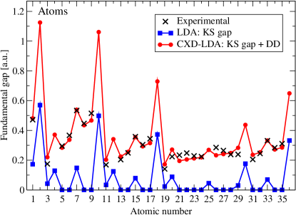
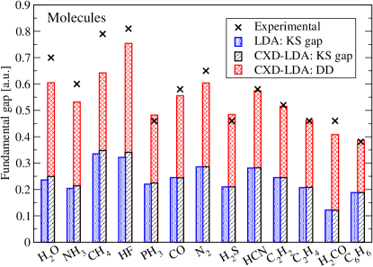
Figure 3: Comparison of the CXD-LDA gap with LDA and available experimental results. The CXD-LDA gap has contributions from the Kohn-Sham (KS) gap and the derivative discontinuity (DD). Result for atoms (top) from H to Kr, experimental values from Ref. NIST , and a set of molecules (bottom), experimental values compiled in Ref. All2002MP , except for C₆H₆ NIST ; Bur1987JCP . (Data in supp. mat. suppmat .)

While the correction has little effect on the KS gap, it changes the KS eigenvalues. This can be seen in the ionization energy (I), which in DFT is given by $-\epsilon_{\mathrm{HOMO}}$ Alm1985PRB . In Fig. 4, we plot I for the LDA and CXD-LDA functionals as a function of the experimental value. In Table 2, we compare the deviation from experimental results for atoms with other XC functionals that have the proper asymptotic limit: LB, RPP, and KLI with Colle-Salvetti correlation Col1975TCA (KLI-CS). The correction procedure improves considerably the LDA results, with similar accuracy to other long range XC potentials.

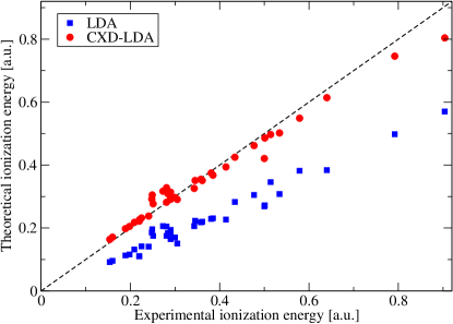
Figure 4: LDA and CXD-LDA ionization energy as a function of the experimental value. Atoms from H to Sr. (Data in supp. mat. suppmat .)

Table 2: Mean absolute error in the ionization energy for atoms (He to Ar). Comparison of CXD-LDA with LDA, LB Van1994PRA , RPP Ras2010JCP and KLI-CS Kri1992PRA ; Col1975TCA functionals. ^aResults from Ref. Oli2010JCTC . ^bResults from Ref. Gra1995CPL given in Ref. Oli2010JCTC . (Data in supp. mat. suppmat .)

LDA	LBa	RPPa	KLI-CSb	CXD-LDA
41%	3.7%	7.4%	5.7%	4.1%

In summary, we have introduced a new auxiliary quantity, the XC density, to construct approximations for the XC potential. Based on an exact condition that the XC potential must fulfill and basic notions of electrostatics, we have presented a correction method for any previously proposed XC potential.

Additionally, the correction procedure allows for the direct calculation of the DD of the XC energy, which can be used to directly predict the fundamental gap as a ground-state property. Moreover, our approach allows for a routine computation of the DD as a practical method for the prediction of the gap.

The proposed potential is a pure functional of the electronic density with a certain degree of non-locality included by the optimization of $\eta_{0}$ and by the Poisson equation. The correction procedure does not depend on any empirical or globally adjusted parameter.

Since the basis for our method is the correction of the XC potential in the asymptotic region, it is not directly applicable to crystalline systems. However, the concepts of the XC density and the DD as a potential shift are still valid. Therefore, it might be possible to generalize the method to solids, where the determination of accurate gaps is one of the main challenges for DFT.

Appendix A Supplementary Material

A.1 Analytic expression for the XC density

Given an XC potential, the XC density is given by

$$n_{\mathrm{xc}}[n]({\bm{r}})=-\frac{1}{4\pi}\nabla^{2}V_{\mathrm{xc}}[n]({\bm{r}})\ ,$$ (12)

by using the chain rule for functional derivatives

$$n_{\mathrm{xc}}[n]({\bm{r}})=-\frac{1}{4\pi}\left[\int\mathrm{d}{\bm{r}}^{\prime}f_{\mathrm{xc}}[n]({\bm{r}},{\bm{r}}^{\prime})\nabla^{2}n({\bm{r}}^{\prime})\right.+\\ \left.+\int\mathrm{d}{\bm{r}}^{\prime}\mathrm{d}{\bm{r}}^{\prime\prime}k_{\mathrm{xc}}[n]({\bm{r}},{\bm{r}}^{\prime},{\bm{r}}^{\prime\prime})\,{\bm{\nabla}}n({\bm{r}}^{\prime})\cdot{\bm{\nabla}}n({\bm{r}}^{\prime\prime})\right]\ ,$$ (13)

where $f_{\mathrm{xc}}$ and $k_{\mathrm{xc}}$ are, respectively, the first and second functional derivatives of $V_{\mathrm{xc}}$ with respect to the density. Interestingly, Eqs. (12) and (13) give a recipe to reconstruct an XC potential from its first two functional derivatives.

A.2 Proof of the conditions for the XC density

The asymptotic condition for $V_{\mathrm{xc}}$ implies that there exists a certain $r_{c}$ such that

$$V_{\mathrm{xc}}({\bm{r}})=-\frac{1}{\left|{\bm{r}}\right|}\quad(\left|{\bm{r}}\right|\geq{\bm{r}_{c}})\ .$$ (14)

If we apply the Laplacian over this equality, we get

$$n_{\mathrm{xc}}({\bm{r}})=0\quad(\left|{\bm{r}}\right|\geq{\bm{r}_{c}})\ ,$$ (15)

the localization condition.

For the normalization condition, we integrate Eq. (12) over a spherical volume of radius $r_{c}$ and we use Gauss’s theorem over the right-hand side

$$\int_{r_{c}\geq r}\mathrm{d}{\bm{r}}\,n_{\mathrm{xc}}({\bm{r}})=-\frac{1}{4\pi}\oint_{r_{c}=r}\mathrm{d}{\bm{A}}\cdot\nabla V_{\mathrm{xc}}({\bm{r}}).$$ (16)

From Eq. (14), $\nabla V_{\mathrm{xc}}[n]=\hat{r}/r^{2}$ which is constant over the sphere, so the integral on the right is just $1/r_{c}^{2}$ times the surface of the sphere, $4\pi r_{c}^{2}$. The integral on the left hand size can be extended to whole space due to Eq. (15), so finally

$$\int\mathrm{d}{\bm{r}}\,n_{\mathrm{xc}}({\bm{r}})=-1\ .$$ (17)

A.3 Optimization of the $\eta$ parameter

Given a XC density $\bar{n}_{\mathrm{xc}}$, the corrected XC density is defined as

$$n_{\mathrm{xc}}({\bm{r}})=\bar{n}_{\mathrm{xc}}({\bm{r}})+\frac{1}{\left|q_{\mathrm{xc}}(\eta)\right|}\Delta n_{\mathrm{xc}}({\bm{r}},\eta)\ ,$$ (18)

with the correction XC density

$$\Delta n_{\mathrm{xc}}[n]({\bm{r}},\eta)=\ \left\{\begin{array}[]{ll}0&\mbox{if }n({\bm{r}})\geq\eta\\ -\bar{n}_{\mathrm{xc}}[n]({\bm{r}})&\mbox{if }n({\bm{r}})<\eta\end{array}\right.\ ,$$ (19)

and the total XC charge

$$q_{\mathrm{xc}}(\eta)=\int\mathrm{d}{\bm{r}}\,\left\{\bar{n}_{\mathrm{xc}}[n]({\bm{r}})+\Delta n_{\mathrm{xc}}[n]({\bm{r}},\eta)\right\}\ .$$ (20)

The value of $\eta$ is optimized for each density, the optimum value $\eta_{0}$ is the value that has the total charge closest to -1. Formally,

$$\eta_{0}[n]=\min_{\eta\leq\eta_{m}}\left|q_{\mathrm{xc}}[n](\eta)+1\right|$$ (21)

where $\eta_{m}$ is the smallest value where $q_{\mathrm{xc}}(\eta)$ has a minimum. These conditions are necessary, since it is not always possible to find a unique value where $q_{\mathrm{xc}}(\eta)=-1$. This can be seen in Fig. 5 were we show $q_{\mathrm{xc}}(\eta)$ for two systems. While for beryllium $q_{\mathrm{xc}}$ never reaches -1, for benzene there are two points where it does. The marks in the figure indicate the value of $\eta_{0}$ and $q_{\mathrm{xc}}(\eta_{0})$ selected by our method.

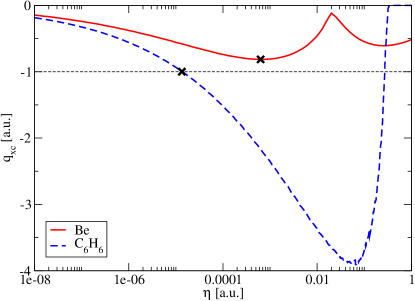
Figure 5: The $q_{\mathrm{xc}}(\eta)$ function, Eq. (20), for LDA on atomic Beryllium atom and C₆H₆. The crosses mark the position of $\eta_{0}$, the optimal value of $\eta$.

A.4 Corrected functional test

To test the corrected LDA functional, CXD-LDA, we did calculations for atomic systems from hydrogen to strontium and for a set of molecules.

The optimized parameter $\eta_{0}$ obtained for each system is plotted Figs. 6 and Figs. 7. For atoms we also plot the corresponding value of $q_{\mathrm{xc}}(\eta_{0})$ and $r_{c}$, the value where $n(r_{c})=\eta_{o}$, that marks the position where the XC density is set to zero. For all tested molecules $q_{\mathrm{xc}}(\eta_{0})=-1$. In Fig. 8, we plot the XC potential for He compared with other functionals. In Fig. 10, we present a more detailed version of the plot for the band gap of the atoms. Finally, we give the values for our optimized parameters, ionization energies and gaps in Tables 4 (molecules) and 5 (atoms).

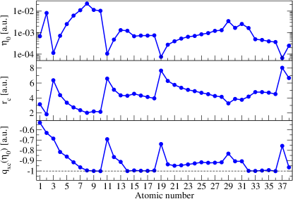
Figure 6: CXD-LDA optimized parameters for atoms. Top: the density threshold $\eta_{0}$. Center: the radius $r_{c}$ where $n(r_{c})=\eta_{0}$. Bottom: The value of the optimized total XC charge, $q_{\mathrm{xc}}(\eta_{0})$.

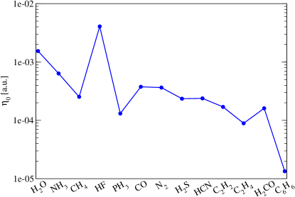
Figure 7: Optimized density threshold, $\eta_{o}$, for a set of small molecules. The value of the total XC charge, $q_{\mathrm{xc}}(\eta_{0})$, is -1 for all cases. Values are given in Table 4.

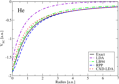
Figure 8: CXD-LDA potential for helium. Comparison with the LDA, LB Van1994PRA , RPP Ras2010JCP and the exact Zha1994PRA potentials.

A.5 Shape of the correction

In Fig. 9 we plot the difference of the corrected XC potential and the original one for 5 atoms and 2 molecules. For atoms the correction has the shape expected from electrostatic principles. For molecules, the correction in the central region is not exactly constant. This is expected as the $n=\eta_{0}$ surface is not necessarily a perfect sphere. However the deviation from a constant shift is not large and we can still obtain a representative value from the average. Near the atomic positions there are some peaks due to numerical error in the finite difference calculation of the Laplacian, but these are a few points that do not influence considerably the average.

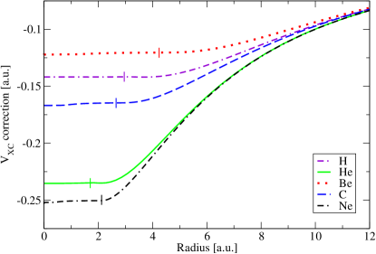
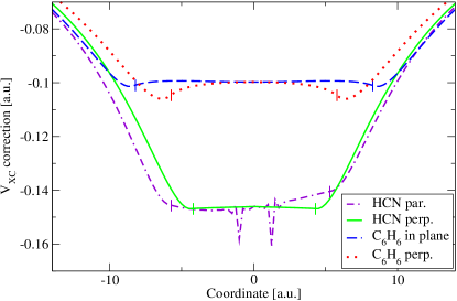
Figure 9: Correction of the LDA X potential for different atoms (top) and molecules (bottom). The vertical lines mark the position where $n=\eta_{0}$. For the HCN molecule the value of the shift is plotted for the axis that passes by the atoms (HCN par.) and other axis that is perpendicular to that one (HCN perp.). For C₆H₆ one axis in the plane of the molecule (C₆H₆ in plane) and the other is perpendicular to that plane (C₆H₆ perp.).

A.6 Alternative calculation of the derivative discontinuity

We propose to calculate the derivative discontinuity (DD) from the shift of the potential due to the correction procedure

$$\Delta_{\mathrm{xc}}^{V}=-\frac{2}{\Omega}\int_{n({\bm{r}})\geq\eta}\mathrm{d}{\bm{r}}\left[V_{\mathrm{xc}}({\bm{r}})-\bar{V}_{\mathrm{xc}}({\bm{r}})\right]\ .$$ (22)

Alternatively, the DD can be obtained by comparing the results of the corrected XC potential with the results of the uncorrected functional. In principle, in DFT the ionization energy is given by the highest occupied Kohn-Sham eigenvalue

$$\epsilon_{\mathrm{HOMO}}=-I\ ,$$ (23)

however, for a potential that averages over the discontinuity All2002MP

$$\bar{\epsilon}_{\mathrm{HOMO}}=-I+\frac{1}{2}\Delta_{\mathrm{xc}}\ .$$ (24)

So, the DD is also given by

$$\Delta_{\mathrm{xc}}^{\epsilon}=2(\bar{\epsilon}_{\mathrm{HOMO}}-\epsilon_{\mathrm{HOMO}})\ .$$ (25)

In table 3 we give the values of the DD obtained with the two previously mentioned approaches, Eq. (22) and Eqs. (23) and (24), for four different atoms.

Atom	$\Delta_{\mathrm{xc}}^{\epsilon}$	$\Delta_{\mathrm{xc}}^{V}$
B	0.281	0.284
C	0.333	0.337
O	0.427	0.435
F	0.460	0.467

Table 3: Comparison of methods to calculate the derivative discontinuity, Eq. (22) and Eq. (25).

A.7 Computational cost of the correction

In general the cost of the correction procedure is not significant in comparison to the total cost of a DFT self-consistent procedure. The additional cost comes from the numerical solution of Eq. (12). This is the same procedure required to obtain the Hartree potential and can be done efficiently in linear or quasi-linear computational time using methods like fast Fourier transforms, multigrid or fast multipole expansions. Moreover, due to linearity, it would be possible to solve the Poisson equation once, obtaining at the same time the Hartree and the corrected XC potentials.

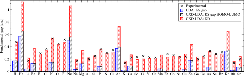
Figure 10: Comparison of fundamental gap calculations with available LDA and CXD-LDA functionals with experimental results for atoms between H and Sr. Experimental values obtained from Ref. NIST . Values are given in Table 5.

Molecule	Experimentala	LDA		CXD-LDA
	$E_{g}$	$\Delta_{\mathrm{ks}}$	$\Delta E_{g}\ \%$	$\eta_{0}$	$\Delta_{\mathrm{ks}}$	$\Delta_{\mathrm{xc}}$	$E_{g}$	$\Delta E_{g}\ \%$
H2O	0.70	0.236	66	1.5E-03	0.249	0.356	0.605	13.6
NH3	0.60	0.204	66	6.4E-04	0.214	0.317	0.532	11.4
CH4	0.79	0.335	58	2.5E-04	0.348	0.294	0.642	18.8
HF	0.81	0.322	60	4.1E-03	0.341	0.413	0.754	6.9
PH3	0.46	0.220	52	1.3E-04	0.225	0.256	0.482	4.7
CO	0.58	0.245	58	3.8E-04	0.244	0.312	0.556	4.1
N2	0.65	0.286	56	3.7E-04	0.286	0.318	0.604	7.1
H2S	0.46	0.210	54	2.3E-04	0.210	0.274	0.484	5.2
HCN	0.58	0.281	52	2.4E-04	0.282	0.292	0.574	1.1
C2H2	0.52	0.245	53	1.7E-04	0.245	0.270	0.515	0.9
C2H4	0.46	0.207	55	8.9E-05	0.208	0.255	0.463	0.6
H2CO	0.46	0.122	74	1.6E-04	0.121	0.287	0.408	11.3
C6H6	0.38	0.188	51	1.3E-05	0.188	0.199	0.386	1.4

Table 4: Experimental, LDA and CXD-LDA results for a set of molecules. $\eta_{0}$: optimized density threshold value from Eq. (19), in all cases $q_{\mathrm{xc}}(\eta_{0})=-1$. $\Delta_{\mathrm{ks}}$: HOMO-LUMO gap, $\Delta_{\mathrm{xc}}$: derivative discontinuity, $E_{g}$: fundamental gap, for CXD-LDA is $\Delta_{\mathrm{ks}}+\Delta_{\mathrm{xc}}$, and $\Delta E_{g}$: Difference in the gap with experimental results, for LDA $\Delta_{\mathrm{ks}}$ is considered as the gap. All calculation are done with the Octopus code Cas2006PSSB using a grid composed of spheres of radius 16 a.u. around each atom with uniform spacing 0.25 a.u, and LDA norm-conserving pseudo-potentials. Geometries from Ref. Cur1997JCP . ^a Experimental values compiled in Ref. All2002MP , except for C₆H₆ obtained as difference between the ionization energy and the electron affinity from Refs. NIST ; Bur1987JCP .

Atom	Experimentala		LDA				CXD-LDA
	$I$	$E_{g}$	$\epsilon_{\mathrm{homo}}$	$\Delta I\ \%$	$\Delta_{\mathrm{ks}}$	$\Delta E_{g}\ \%$	$\eta_{0}$	$q_{\mathrm{xc}}(\eta_{0})$	$\epsilon_{\mathrm{homo}}$	$\Delta I\ \%$	$\Delta_{\mathrm{ks}}$	$\Delta_{\mathrm{xc}}$	$E_{g}$	$\Delta E_{g}\ \%$
H	0.500	0.472	-0.269	46	0.173	63	6.8E-04	-0.53	-0.421	15.8	0.174	0.307	0.481	2.0
He	0.904	–	-0.570	37	0.570	–	8.2E-03	-0.63	-0.804	11.0	0.655	0.470	1.125	–
Li	0.198	0.175	-0.116	41	0.042	76	1.1E-04	-0.69	-0.205	3.5	0.043	0.177	0.220	25.4
Be	0.343	–	-0.206	40	0.129	–	7.1E-04	-0.82	-0.326	4.8	0.129	0.241	0.371	–
B	0.305	0.295	-0.151	51	0.000	100	2.5E-03	-0.86	-0.291	4.5	0.000	0.284	0.284	3.5
C	0.414	0.367	-0.227	45	0.000	100	6.2E-03	-0.92	-0.394	4.8	0.000	0.337	0.337	8.2
N	0.534	0.534	-0.308	42	0.148	72	1.1E-02	-0.96	-0.502	6.1	0.148	0.391	0.539	0.9
O	0.501	0.447	-0.272	46	0.000	100	2.2E-02	-1.00	-0.486	2.9	0.000	0.435	0.435	2.7
F	0.640	0.515	-0.384	40	0.000	100	1.1E-02	-1.00	-0.614	4.1	0.000	0.467	0.467	9.4
Ne	0.792	–	-0.498	37	0.498	–	1.0E-02	-1.00	-0.746	5.9	0.560	0.501	1.061	–
Na	0.189	0.169	-0.113	40	0.034	80	1.1E-04	-0.69	-0.198	4.7	0.034	0.169	0.203	20.5
Mg	0.281	–	-0.175	38	0.125	–	4.7E-04	-0.86	-0.282	0.5	0.126	0.215	0.341	–
Al	0.220	0.204	-0.111	50	0.000	100	1.3E-03	-0.91	-0.222	0.8	0.000	0.224	0.224	9.8
Si	0.300	0.249	-0.170	43	0.000	100	1.2E-03	-1.00	-0.297	1.0	0.000	0.256	0.256	2.9
P	0.385	0.358	-0.231	40	0.079	78	6.8E-04	-1.00	-0.368	4.5	0.080	0.275	0.355	0.9
S	0.381	0.304	-0.229	40	0.000	100	7.3E-04	-1.00	-0.375	1.6	0.000	0.293	0.293	3.6
Cl	0.477	0.344	-0.305	36	0.000	100	7.3E-04	-1.00	-0.462	3.0	0.000	0.315	0.315	8.5
Ar	0.579	–	-0.382	34	0.373	–	7.4E-04	-1.00	-0.549	5.2	0.394	0.335	0.729	–
K	0.160	0.141	-0.096	40	0.023	84	7.5E-05	-0.74	-0.171	6.9	0.023	0.149	0.172	22.2
Ca	0.225	0.224	-0.142	37	0.088	61	2.7E-04	-0.94	-0.232	3.4	0.089	0.182	0.271	21.0
Sc	0.241	0.234	-0.141	42	0.000	100	4.0E-04	-0.95	-0.238	1.1	0.000	0.195	0.195	16.6
Ti	0.251	0.248	-0.175	30	0.000	100	5.3E-04	-0.95	-0.277	10.2	0.000	0.205	0.205	17.3
V	0.248	0.229	-0.186	25	0.000	100	6.4E-04	-0.94	-0.292	17.8	0.000	0.212	0.212	7.1
Cr	0.249	0.224	-0.196	21	0.000	100	7.0E-04	-0.93	-0.305	22.7	0.000	0.219	0.219	2.3
Mn	0.273	–	-0.206	25	0.045	–	8.4E-04	-0.92	-0.317	16.1	0.045	0.224	0.269	–
Fe	0.290	0.285	-0.183	37	0.000	100	9.5E-04	-0.92	-0.299	2.9	0.000	0.233	0.233	18.2
Co	0.290	0.265	-0.194	33	0.000	100	1.2E-03	-0.92	-0.314	8.5	0.000	0.241	0.241	9.2
Ni	0.281	0.238	-0.205	27	0.000	100	1.3E-03	-0.92	-0.328	16.7	0.000	0.248	0.248	4.0
Cu	0.284	0.239	-0.184	35	0.030	88	3.4E-03	-0.83	-0.309	8.8	0.030	0.253	0.283	18.5
Zn	0.345	–	-0.223	35	0.176	–	1.7E-03	-0.91	-0.351	1.8	0.178	0.259	0.437	–
Ga	0.220	0.205	-0.110	50	0.000	100	2.5E-03	-0.91	-0.226	2.3	0.000	0.236	0.236	15.2
Ge	0.290	0.245	-0.165	43	0.000	100	1.6E-03	-1.00	-0.291	0.1	0.000	0.253	0.253	3.2
As	0.361	0.331	-0.220	39	0.070	79	4.9E-04	-1.00	-0.351	2.7	0.070	0.262	0.332	0.5
Se	0.358	0.284	-0.218	39	0.000		4.6E-04	-1.00	-0.355	1.0	0.000	0.272	0.272	4.3
Br	0.434	0.311	-0.283	35	0.000	100	3.9E-04	-0.99	-0.425	2.1	0.000	0.285	0.285	8.2
Kr	0.514	–	-0.346	33	0.332	–	3.6E-04	-1.00	-0.497	3.4	0.347	0.302	0.649	–
Rb	0.154	0.136	-0.092	40	0.020	85	6.6E-05	-0.76	-0.164	6.7	0.020	0.144	0.164	21.0
Sr	0.209	0.207	-0.132	37	0.070	66	2.5E-04	-0.96	-0.218	4.0	0.070	0.172	0.242	16.9

Table 5: Experimental, LDA and CXD-LDA results for atomic systems. $\eta_{0}$: optimized density threshold value from Eq. (19), $q_{\mathrm{xc}}(\eta_{0})$: optimized value of the total XC charge [Eq. (20)], $\epsilon_{\mathrm{HOMO}}$: HOMO eigenvalue, $I$: Ionization energy, $\Delta I$: difference between $-\epsilon_{\mathrm{HOMO}}$ and the experimental $I$, $\Delta_{\mathrm{ks}}$: HOMO-LUMO gap, $\Delta_{\mathrm{xc}}$: derivative discontinuity, $E_{g}$: fundamental gap, for CXD-LDA is $\Delta_{\mathrm{ks}}+\Delta_{\mathrm{xc}}$, and $\Delta E_{g}$: difference in the gap with experimental results, for LDA $\Delta_{\mathrm{ks}}$ is considered as the gap. Values calculated using the APE code Oli2008CPC with spin-polarization. ^a Experimental results from Ref. NIST , $E_{g}$ values calculated as the difference of the ionization energy and the electron affinity.