Theory of quantum energy transfer in spin chains: From superexchange to ballistic motion

Abstract

Quantum energy transfer in a chain of two-level (spin) units, connected at its ends to two thermal reservoirs, is analyzed in two limits: (i) In the off-resonance regime, when the characteristic subsystem excitation energy gaps are larger than the reservoirs frequencies, or the baths temperatures are low. (ii) In the resonance regime, when the chain excitation gaps match populated bath modes. In the latter case the model is studied using a master equation approach, showing that the dynamics is ballistic for the particular chain model explored. In the former case we analytically study the system dynamics utilizing the recently developed Energy-Transfer Born-Oppenheimer formalism [Phys. Rev. E 83, 051114 (2011)], demonstrating that energy transfers across the chain in a superexchange (bridge assisted tunneling) mechanism, with the energy current decreasing exponentially with distance. This behavior is insensitive to the chain details. Since at low temperatures the excitation spectrum of molecular systems can be truncated to resemble a spin chain model, we argue that the superexchange behavior obtained here should be observed in widespread systems satisfying the off-resonance condition.

I Introduction

The scaling of the energy current with system size is of interest for developing applications in energy conversion Rachel , molecular electronics MolEl , and reaction dynamics Rdyn . In the context of biological macromolecules, understanding pathways and efficiency of heat flow is important for controlling signal transmission and functionality in biomolecules Leitnerbook . In nanoscale electric devices significant power dissipation may lead to the system disintegration. Designing efficient routes for energy transfer, away from the conducting object, is essential for a stable operation Pop .

Resolving the size effect of heat conduction in molecular chains has been the subject of recent experiments Schwarzer ; Segalman . For example, Wang et al. DlottE has recently studied the kinetics of heat transfer from a metal substrate to self-assembled hydrocarbon monolayers of increasing sizes DlottRev , concluding that heat travels ballistically along the chain SegalHeat . Vibrational energy transport in peptide helices was measured by employing vibrational probes as local thermometers at various distances from a heat source Hamm . For this protein system it was concluded that heat propagates in a diffusive-like process.

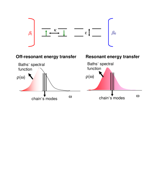
Figure 1: Top: Chain of two-level particles or spin-1/2 objects coupled at the edges to heat baths maintained at different temperatures. Bottom: In the off-resonance regime, applicable, e.g., at low temperatures, the chain’s modes, relevant for the transport process, match unpopulated bath modes. In the opposite resonance regime the chain’s modes overlap with populated bath modes. The coloring of the baths’ spectral function represents thermal population, where darker color reflects larger occupation. The off-resonant model could be also realized considering reservoirs whose spectral functions have a low cutoff, below the chain’s characteristic excitation gaps.

Considering electron transfer across a 1-dimensional (1D) conductor (bridge) connected at the edges to electron reservoirs, multitude of theoretical, numerical, and experimental studies have demonstrated that in the resonance limit, applicable for ohmic reservoirs at high temperatures, (quasi) 1D chains conduct electrons anywhere between a ballistic to a diffusive manner, depending on the details of the internal interactions. In contrast, in the off-resonance regime, when the electronic levels of the bridge lie high, above the populated states of the reservoirs (the donor and acceptor states in a donor-bridge acceptor complex), a deep tunneling mechanism should take off NitzanRev .

In this paper we focus on the analogous problem of energy transfer in molecular chains connected at the two ends to thermal reservoirs (baths), maintained at distinct temperatures, realized by solids, metals, nanoparticles HammNP or large molecular complexes Schwarzer . As a simple model for the central object we consider a chain of several two-level units (spin 1/2 particles). The units are coupled through nearest-neighbor coupling terms, assumed to be weak compared to the on-site energies. Similarly to the electronic case, we expect that distinct transport mechanisms will dominate at different parameter regimes. For a schematic representation of the chain model and the relevant excitation spectra see Fig. 1.

Before proceeding, we carefully clarify our terminology: ”Resonant” regime refers here to the case where the modes of the chain, responsible for the heat transfer dynamics, lie in resonance with the occupied baths’ modes. In contrast, ”Off-Resonance” conduction refers to the case where the occupied modes of the thermal reservoirs’ are low, below the typical excitation frequencies of the enclosed object. Overall, there is always a conservation of energy in our system, transferred between the two reservoirs (donor and acceptor). Thus, irrespective of the bridge energetics, we always consider here a ”resonance energy transfer” (RET) process Scholes ; EET , in the sense that there are no energy loss mechanisms, e.g., it is a non-radiative process.

In the resonant regime numerous theoretical and computational studies have demonstrated that energy transfer between two reservoirs, mediated by the excitation of the interlocated object, may follow a ballistic $J\propto N^{0}$, ohmic $J\propto N^{-1}$, (or somewhere in between, $J\propto N^{\alpha-1}$, $\alpha>0$) mechanism. This was done in the context of vibrational energy transfer Dhar and thermal transport in spin chain Brenig ; Prosen ; ProsenM , for both classical and quantum systems, using, e.g., molecular dynamics simulations Dhar , the quantum master equation method Gemmer ; ProsenM ; Mona , the Green-Kubo formula Saito ; MichelKubo , and the density matrix renormalization group method DMRG . In the off-resonant regime simulations on purely harmonic systems indicated on a tunneling dynamics of heat transfer SegalHeat . In the presence of interactions, off-resonant quantum heat transfer dynamics has been treated by adopting e.g., the complex machinery of the Green’s function approach Green1 ; Green2 , or by using mixed quantum-classical simulations Stock . Typically, such methods only provide numerical results, hindering direct picture of the microscopic processes involved. Responding to this challenge, we have recently developed a simple analytic method for describing energy transfer in nonlinear systems in the off-resonant regime BOheat . This method, an extension of the Born-Oppenheimer (BO) principle BO to energy transfer problems, can treat general subsystems (impurity, chains) with intrinsic anharmonicities, as well as cases where the subsystem is nonlinearly coupled to the reservoirs. The outcome of the method is a Landauer type expression, incorporating nonlinear interactions Land , allowing for the identification of different scattering processes BOheat . In what follows we refer to this method as the Energy-Transfer Born-Oppenheimer (ETBO) scheme.

In this paper we aim in deriving scaling laws for the behavior of the energy current with size for 1D molecular systems, primarily focusing on the off-resonant limit comment . For simplicity, we consider the isotropic XY spin chain and its variants as a prototype for a homogeneous and linear molecular chain commXY . This is a relevant physical description since at low temperatures or in the off-resonance limit the energy spectra of the interlocated system can be truncated, as transport predominantly occurs through the lowest excitation states. Considering a spin chain between two thermal reservoirs, we study the energy transfer behavior in two different limits: (i) We assume an off-resonance scenario, and obtain the energy current adopting the ETBO approach. In this case we demonstrate that the energy current decays exponentially with size, a footprint of the tunneling mechanism. (ii) In a resonant situation we utilize a standard master equation approach and show that the isotropic XY chain behaves as a ballistic conductor, providing a fixed current for different sizes. While we present our study in the context of steady state heat transfer, the results are also useful for interpreting energy transfer rates in donor-bride-acceptor complexes Nitzan

The tunneling behavior of the energy current resolved in the off-resonance regime Speiser ; Scholes ; EET resembles the McConnell superexchange result superEx , observed in electron transport experiments in numerous systems, including monolayers Mono , proteins Protein , and DNA DNA . Since the thermal superexchange result does not depend on the details of the chain model, we expect it to show up in different physical systems at low temperatures, including molecular wires, spin chains, and biomolecules.

Our study here is presented in the context of thermal energy transfer. However, the analysis and results are valid for describing general excitation energy transfer problems (vibrational, electronic), in bulk-molecule-bulk junctions and donor-bridge-acceptor systems Speiser ; Scholes ; EET . Experiments on $\sigma$-bond or $\pi$-bond bridges, connected to donor and acceptor chromophores reported on excitation transfer rates which are exponentially decreasing with size EETexp ; EETratner . This behavior is rigorously recovered here.

The structure of this paper is as follows. In Section II we describe the spin chain model, serving as a prototype for studying energy transfer and thermal conduction in linear chains. In Section III we study the off-resonant case using the ETBO method. Perturbative analytic results are supported by numerical simulations. Section IV treats the resonant limit, adopting a master equation approach. Section V concludes.

Figure 2: Energy spectrum of the isolated isotropic XY spin chain with $N=2$, $N=4$, $N=6$, and $N=8$ units. Other parameters are $\epsilon=2$ and $\kappa=0.1$. The different manifolds include different numbers of excitations on the chain, from zero up to $N$.

Figure 3: Energy spectrum of the isolated anisotropic Heisenberg spin chain with $N=4$ (a) and $N=10$ (b). Panel (c) zooms on a small portion of the spectrum for $N=10$, manifesting the gap closure with increasing $\delta$. Other parameters are $\epsilon=2$, $\kappa=0.1$ and $\delta=0$ ($\circ$), $\delta=1$ ($+$) and $\delta=2$ (dotted).

II Model

Consider a small subsystem, representing e.g., a molecule, placed in between two thermal reservoirs (e.g., solids, large complexes) maintained each at a fixed temperature $T_{\nu}=\beta_{\nu}^{-1}$ ($\nu=L,R$). The total Hamiltonian is given by

$$H=H_{S}+H_{L}+H_{R}+V_{L}+V_{R}.$$ (1)

$H_{S}$ is the Hamiltonian of the subsystem and $H_{\nu}$ stands for the $\nu$ heat bath. $V_{\nu}$ couples the subsystem and the $\nu$ reservoir. In particular, in what follows we focus on the thermal transport properties of the isotropic XY spin-chain commXY

$$H_{S}=\frac{\epsilon}{2}\sum_{j=1}^{N}\sigma_{j}^{z}+\frac{\kappa}{2}\sum_{j=1}^{N-1}\left(\sigma_{j}^{x}\sigma_{j+1}^{x}+\sigma_{j}^{y}\sigma_{j+1}^{y}\right).$$ (2)

Here $\sigma_{j}^{x,y,z}$ are the Pauli matrices for the $j$ spin. The first term describes the onsite spectrum at each site, a two level system with a spacing $\epsilon$. The second term provides the hopping interaction between neighboring sites with an exchange strength $\kappa$. We generally assumes that $\kappa<\epsilon$, allowing for a meaningful description of the chain in terms of its subunits. The chain is coupled to two independent thermal reservoirs at sites $1$ and $N$. Our derivation below does not make any assumption regarding the structure of these baths. For example, they may each contain a collection of independent harmonic oscillators

$$H_{\nu}=\sum_{j\in\nu}\omega_{j}b_{\nu,j}^{\dagger}b_{\nu,j}.$$ (3)

One may also consider fermionic reservoirs, a source of electronic excitations. System-bath interactions are assumed to take the following form,

$$V_{L} = S_{1}B_{L};\,\,\,\,S_{1}=\lambda_{L}\sigma_{1}^{x}$$

$$V_{R} = S_{N}B_{R};\,\,\,\,S_{N}=\lambda_{R}\sigma_{N}^{x},$$ (4)

where $\lambda_{\nu}$ parametrizes the system-bath coupling strength, assumed to be a real number, $S_{1}$ ($S_{N}$) are subsystem operators coupled to the left (right) reservoirs, $B_{L}$ ($B_{R}$) are $L$ ($R$) bath operators, which need not be specified at this stage. This form assumes that the interaction with the reservoirs can generate (absorb) an excitation at the leftmost or rightmost sites of the chain.

Using the Jordan-Wigner transformation Jordan , the (isolated) isotropic XY chain can be reduced to describe spinless free fermions. However, our analysis is still not trivial since the chain is coupled, potentially in a nonlinear way, to thermal reservoirs which are not necessarily modeled by isotropic XY chains by themselves. Thus, the total Hamiltonian cannot be transformed into a collection of noninteracting fermions, and the model is generally non-integrable. Furthermore, the ETBO analysis can be carried out for studying transport through the 1D anisotropic Heisenberg model commXY ,

$$H_{S}=\frac{\epsilon}{2}\sum_{j=1}^{N}\sigma_{j}^{z}+\frac{\kappa}{2}\sum_{j=1}^{N-1}\left(\sigma_{j}^{x}\sigma_{j+1}^{x}+\sigma_{j}^{y}\sigma_{j+1}^{y}\right)+\frac{\kappa\delta}{2}\sigma_{j}^{z}\sigma_{j+1}^{z}.$$ (5)

The spectrum of $H_{S}$ with $\delta=0$ is exemplified in Fig. 2 for several sizes. We note that for $\epsilon\gg\kappa$ subsystem energies are grouped into manifolds, each including eigenstates with a particular number of excitations: At the bottom of the spectrum lies a zero excitation state with an energy of $E_{0}\sim(-\frac{N}{2}\epsilon)$. Above, we identify states including a single excitation on the chain, with their energy centered around $E_{0}+\epsilon$. The next manifold includes the two-excitation states, and so on and so forth. For example, for $N=4$ there are five manifolds with zero (bottom) to four (top) excitations residing on the chain. Note that given the form of the system-bath interaction operator [Eq. (4)], the thermal baths, the excitation resources, can only translate the subsystem between (neighboring) manifolds, adding or absorbing a single excitation at a time. The reservoirs cannot directly drive transitions within each manifold. Since for $\kappa\ll\epsilon$ the typical gap between manifolds is $\sim\epsilon$, this energy scale is identified as the characteristic frequency of the subsystem, controlling the transport properties of the model.

In Fig. 3 we show that this picture is retained when the exchange anisotropy parameter $\delta$ is relatively small, for short chains. Then, one can still identify manifolds with different number of excitations, as the gap between bands is larger than energy differences within each band. However, for large $\delta$ and for long chains the spectrum becomes more involved, and the gaps between different excitation states diminish. In what follows we restrict ourselves to situations where the gaps between manifolds are maintained, $\sim\epsilon$, larger than the spacings within each band (bandwidth $\sim\kappa$). Practically, we study chains of $N<10$ units, with large onsite gaps $\epsilon\gg\kappa$ and small anisotropy parameter $0<\delta<1$.

The spin chain serves as a prototype model for exploring energy transfer through a linear molecular junction, at low temperatures. In what follows we study the steady state behavior of this model in two different limits:

(i) Off-resonance case, with $\epsilon\gg\omega_{c}$ or $T_{\nu}<\epsilon$. Here $\omega_{c}$ is the reservoirs cutoff frequency. In this limit energy transfer takes places between low frequency modes of the two reservoirs, mediated by a (high frequency) subsystem. For treating the dynamics in this scenario, we adopt the recently developed Energy-Transfer Born-Oppenheimer method BOheat . In Sec. III we show that in this regime heat is transferred via a coherent-superexchange mechanism, with the current exponentially decreasing with chain size.

(ii) Resonance regime, with $\epsilon<\omega_{c}$ and $T_{\nu}>\epsilon$. Under these conditions baths’ modes in resonance with the subsystem frequencies are populated, responsible for the subsystem excitation and relaxation processes. This resonance energy transfer process can be treated within the Born-Markov approximation scheme MasterD ; Hyblong . In Sec. IV we show that in this case the isotropic XY model transfers energy in a ballistic manner.

III Off-resonance regime: Energy-Transfer Born-Oppenheimer scheme

III.1 Method

We describe the principles of the Energy-Transfer Born-Oppenheimer method as developed in Ref. BOheat , then apply it onto the spin-chain model, to obtain the behavior of the current as a function of size. Generally, the BO approximation BO is based on the recognition of timescale separation. In isolated molecules, the ”traditional” BO approximation relays on the mass separation of electrons and atomic nuclei. In this context, one assumes that the electron cloud instantly adjusts to changes in the nuclear configuration, and that the nuclei propagate on a single potential energy surface associated with a single electronic quantum state, obtained by solving the Schrodinger equation with fixed nuclear geometries.

This principle can be adopted for treating quantum thermal transport in (potentially strong) interacting systems driven to a steady state by a temperature bias BOheat . The method is applicable in the off-resonant regime, where the characteristic frequencies of the impurity object are high relative to the cutoff frequencies of the reservoirs $\epsilon\gg\omega_{c}$ comment . This implies a timescale separation, as the subsystem dynamics is fast, while the bath motion is slow. The ETBO approximation follows two consecutive steps: First, we consider the fast variable and solve the subsystem eigenproblem while fixing the reservoirs configuration, to acquire a set of potential energy surfaces which parametrically depend on the bath coordinates. In the second step we adopt the adiabatic approximation and assume that the baths’ coordinates, the slow variables, evolve without changes on the subsystem state. We then solve the energy transfer problem between the reservoirs on a fixed potential surface.

In what follows we denote by $q$ subsystem coordinates and by $Q_{\nu}$ the $\nu$ bath coordinates. These are collections of displacements and momenta operators. The baths operators which are coupled to the subsystem, $B_{\nu}$, are functions of the $Q_{\nu}$ coordinates. We also collect in $Q$ the coordinates of both reservoirs. Fixing the bath coordinates, we identify the ’fast’ contribution to Eq. (1) as

$$H_{f}(q,Q)=H_{S}(q)+\sum_{\nu}V_{\nu}(q,Q_{\nu}),$$ (6)

and solve the time-independent Schrödinger equation

$$H_{f}(q,Q)|g_{n}(q,Q)\rangle=W_{n}(Q)|g_{n}(q,Q)\rangle,$$ (7)

to acquire a set of ”potential energy surfaces”, $W_{n}(Q)$, and states $|g_{n}(q,Q)\rangle$. Note that the potentials $W_{n}$ mix the left and right system-bath interaction operators. Moreover, they are not necessarily linear in $Q_{L}$ and $Q_{R}$. These potentials are the analogs of the electronic potential energy surfaces obtained in molecular structure calculations, which parametrically depend on the nuclear coordinates. Similarly, the reservoir coordinates $Q$ are treated as parameters in Eq. (7). Assuming that the surfaces are well separated, we presume the adiabatic ansatz and write the total density matrix as

$$\rho(t)=\left|g_{n}(q,Q)\right\rangle\rho_{B}^{n}(Q,t)\left\langle g_{n}(q,Q)\right|,$$ (8)

where the bath density matrix obeys the Liouville equation

$$\rho_{B}^{n}(Q,t)=e^{-iH_{BO}^{n}t}\rho_{B}(0)e^{iH_{BO}^{n}t},$$ (9)

$\hbar\equiv 1$, with the effective Hamiltonian

$$H_{BO}^{n}=H_{L}(Q_{L})+H_{R}(Q_{R})+W_{n}(Q_{L},Q_{R}).$$ (10)

Here $\rho_{B}(0)=\rho_{L}\times\rho_{R}$ is a factorized initial condition with $\rho_{\nu}=e^{-\frac{H_{\nu}}{T_{\nu}}}/{\rm Tr_{\nu}}\big{[}e^{-\frac{H_{\nu}}{T_{\nu}}}\big{]}$, the equilibrium-canonical distribution function of the $\nu$ bath. In what follows, we assume that the baths coordinates evolve on the ground potential surface, simply denoted by $W$. The effective Hamiltonian (10) including the ground potential surface $W$ will be similarly denoted by $H_{BO}$. For brevity, we also omit references to coordinates. Our plan is to study next the quantum dynamics dictated by the Hamiltonian (10), on a particular surface. Such an analysis is analogous to the investigation of vibrational dynamics on a particular electronic potential surface, in the traditional application of the BO approximation.

In steady state, the energy current operator, e.g., at the $L$ contact, can be defined as Wucurr

$$\hat{J}_{L}=i[H_{L},W],$$ (11)

with the expectation value

$$J_{L}(t)=\text{Tr}[\hat{J}_{L}\rho_{B}(t)]=\text{Tr}[e^{iH_{BO}t}\hat{J}_{L}e^{-iH_{BO}t}\rho_{B}(0)].$$ (12)

The left expression is written in the Schrödinger picture; the second is in the Heisenberg representation. The trace is performed over the two baths’ degrees of freedom. When system-baths couplings, absorbed into $W$, are weak, the time evolution operator can be approximated by the first order term

$$e^{-iH_{BO}t}=e^{-i(H_{L}+H_{R})t}\left(1-i\int_{0}^{t}W(\tau)d\tau\right),$$ (13)

and the current (12) reduces to

$$J_{L}(t)=-i\int_{0}^{t}\text{Tr}\{[\hat{J}_{L}(\tau),W]\rho_{L}\rho_{R}\}d\tau.$$ (14)

Here $W(\tau)$ and $\hat{J}_{L}(\tau)$ are interaction picture operators, $O(t)=e^{iH_{B}t}Oe^{-iH_{B}t}$ with $H_{B}=H_{L}+H_{R}$. We are interested in steady-state quantities, $J=J_{L}(t\rightarrow\infty)$, if the limit exists. Expression (14) can be further customized, recalling the bipartite interaction form of $V_{\nu}$ in the original Hamiltonian (1). Then, one can formally expand $W$ in terms of the bath operators which are coupled to the subsystem, $B_{\nu}$,

$$W = \sum_{a,b}A_{a,b}B_{L}^{a}\otimes B_{R}^{b}$$

$$= \sum_{a,b}\sum_{k,m}\sum_{p,s}A_{a,b}(B_{L}^{a})_{km}(B_{R}^{b})_{ps}\left|kp\right\rangle\left\langle ms\right|.$$

The operators $B_{L}$ and $B_{R}$ depend on the bath coordinates, collected into $Q_{L}$ and $Q_{R}$, respectively. The actual form is not important at this (formal) stage. It is specified only once particular models are constructed, see e.g., Eq. (23). The coefficients $A_{a,b}$ absorb the subsystem parameters, the energies $\epsilon$, $\kappa$ and $\delta$ in the chain model and the system-bath interaction strength $\lambda_{\nu}$. The powers $a$ and $b$ are positive integers. $|k\rangle$ and $|m\rangle$ represent the many body states of the left reservoir with energies $E_{k}$ and $E_{m}$, (i.e. $H_{L}=\sum E_{k}\left|k\right\rangle\left\langle k\right|$). Similarly, $|p\rangle$ and $|s\rangle$ are the many body states of the right reservoir with energies $E_{p}$ and $E_{s}$. Assuming a weak system-bath coupling strength, we truncate $W$ and consider only the lowest order term in $B_{L}B_{R}$,

$$W\sim A_{0,0}+A_{1,1}B_{L}B_{R}+O(B_{L}^{2})+O(B_{R}^{2}).$$ (16)

A more general derivation in presented in Ref. BOheat . It can be shown that only terms containing products of $B_{L}$ and $B_{R}$ add to the current, thus only the second term in Eq. (16) actually matters for the energy current calculations. We also note that $A_{1,1}$ is proportional to the product $\lambda_{L}\lambda_{R}$, see Eq. (4). We therefore define the function $\mathcal{T}(\epsilon,\kappa)$ through the relation

$$A_{1,1}\equiv\lambda_{L}\lambda_{R}\mathcal{T}(\epsilon,\kappa),$$ (17)

where we explicitly indicate its dependence on the subsystem parameters. Back to (14), employing Eqs. (11) and (16), we obtain

$$J = \frac{\mathcal{T}(\epsilon,\kappa)^{2}}{Z_{L}Z_{R}}\int_{0}^{\infty}dt\Big{[}\sum_{k,m}\lambda_{L}^{2}E_{km}e^{iE_{km}t}(B_{L})_{km}(B_{L})_{mk}e^{-\beta_{L}E_{k}}$$ (18)

$$\times\sum_{p,s}\lambda_{R}^{2}(B_{R})_{p,s}(B_{R})_{s,p}e^{iE_{ps}t}e^{-\beta_{R}E_{p}}+c.c.\Big{]},$$

where, e.g., $Z_{L}=\sum_{k}e^{-\beta_{L}E_{k}}$ is the $L$ bath partition function; $\beta_{\nu}=1/T_{\nu}$, $k_{B}\equiv 1$, and $E_{km}=E_{k}-E_{m}$. Time integration can be readily performed, leading to the steady state heat current

$$J=\frac{\mathcal{T}(\epsilon,\kappa)^{2}}{2\pi}\int_{0}^{\infty}\omega d\omega\big{[}k_{L+}(\omega)k_{R-}(\omega)-k_{L-}(\omega)k_{R+}(\omega)\big{]}.$$ (19)

The excitation ($+$) and relaxation ($-$) rate constants are given by

$$k_{L\pm}(\omega)=2\pi\sum_{k,m}\lambda_{L}^{2}[(B_{L})_{km}(B_{L})_{mk}]^{\pm}\delta(E_{k}-E_{m}\mp\omega)\frac{e^{-\beta_{L}E_{k}}}{Z_{L}}.$$ (20)

We have introduced here the short notation $[(B_{L})_{km}(B_{L})_{mk}]^{+}$, to denote matrix elements when $E_{k}>E_{m}$. Similarly, $[(B_{L})_{km}(B_{L})_{mk}]^{-}$ describes the $E_{k}<E_{m}$ case. Analogous expressions hold for the $R$ rates. We can also rewrite the rate constants as Fourier transforms of bath correlation functions

$$k_{L\pm}(\omega)=\lambda_{L}^{2}\int_{-\infty}^{\infty}e^{\mp i\omega t}{\rm Tr}\left[\rho_{L}B_{L}(t)B_{L}(0)\right]dt,$$ (21)

satisfying detailed balance, $k_{L+}(\omega)=k_{L-}(\omega)e^{-\beta_{L}\omega}$. Using this relation, we organize Eq. (19) as

$$J=\frac{\mathcal{T}(\epsilon,\kappa)^{2}}{2\pi}\int_{0}^{\infty}\omega d\omega k_{L-}(\omega)k_{R-}(\omega)(e^{-\beta_{L}\omega}-e^{-\beta_{R}\omega}).$$ (22)

This result is given in the form of a ”generalized Landauer formula”: The net heat current is given as the difference between left-moving and right-moving excitations, nevertheless, unlike the original Landauer formula Land , this expression can incorporate anharmonic effects within the chain model, eventually absorbed into $\mathcal{T}$, and nonlinear system-bath interactions, taken in by the rates $k_{\nu\pm}(\omega)$. We emphasize the broad status of Eq. (22): It does not assume a particular structure for the subsystem, or a specific system-bath interaction form, $B_{\nu}$, both contained inside $W$. It is valid as long as (i) there exists a timescale separation between the subsystem motion (fast) and the reservoirs dynamics (slow), and (ii) system-bath interactions, given in a bipartite form, are weak, see Eqs. (13) and (16).

Eq. (22) readily reveals the dependence of the current on the subsystem parameters, thus it is immensely useful for exploring transport behavior. It includes a product of two terms: The prefactor depends on the subsystem parameters, the integral over frequencies encompasses the bath operators within the Fermi golden rule rates (possibly nonlinear in the bath coordinates). The effect of the reservoirs’ temperatures is enclosed there. Since the prefactor $\mathcal{T}(\epsilon,\kappa)$ is the only term corroborating chain parameters, by obtaining the ground state surface $W$ [Eqs. (16)-(17)], the scaling of the current with size and energy can be gained, without solving a dynamical problem.

We can also regard Eq. (22) as a generalization of the nonadiabatic transition rate, $k_{da}=2\pi|V_{da}|^{2}FCWD$, describing electron or energy transfer processes within a donor-bride-acceptor complex, to current carrying steady state situations. Here, the Franck-Condon factor $FCWD$ accounting for the conservation of energy, depends on the temperature of the environment Scholes . In Eq. (22) this term is portrayed by the frequency integral, considering a transport process originating from a particular state within the $L$ bath. The second part, $V_{da}$, combines the electronic coupling between the donor and acceptor states. In the present work this factor is accounted for by the function $\mathcal{T}(\epsilon,\kappa)$.

As an example of the utility of the ETBO method to describe off-resonance conduction processes, consider a harmonic impurity of frequency $\Omega$, linearly coupled to two harmonic reservoirs,

$$H_{S} = \Omega b^{\dagger}b,$$

$$H_{\nu} = \sum_{j}\omega_{j}b_{\nu,j}^{\dagger}b_{\nu,j},\,\,\,\,\,\,\,V_{\nu}=(b^{\dagger}+b)\lambda_{\nu}B_{\nu}$$ (23)

with $B_{\nu}=\sum_{j}(b_{\nu,j}^{\dagger}+b_{\nu,j})$. Here $b_{\nu,j}^{\dagger}$ ($b_{\nu,j}$) are the creation (annihilation) operators of the mode $j$ in the $\nu$ bath, $b^{\dagger}$ and $b$ are the respective subsystem operators. Since the model is fully harmonic, in principle the energy current can be exactly obtained. However, this calculation requires some effort, and the scaling of the current with size is not easy to reveal SegalHeat ; Dhar . Focusing on the off-resonance limit, the ETBO method can readily provide the behavior of the current at weak couplings. We diagonalize $H_{f}=H_{S}+V$ and resolve the ground potential surface $W=-\frac{2}{\Omega}(\lambda_{L}B_{L}+\lambda_{R}B_{R})^{2}$, thus extract $\mathcal{T}\propto 1/\Omega$. Relaying on the bilinear interaction form, the transition rates (21) can be obtained, $k_{\nu+}(\omega)=\Gamma_{\nu}(\omega)n_{\nu}(\omega)$, where $n_{\nu}(\omega)=[e^{\beta_{\nu}\omega}-1]^{-1}$ is the Bose-Einstein distribution function and the coefficient $\Gamma_{\nu}(\omega)$ incorporates the system-bath interaction strength and the bath’s density of states, assumed to be weak $\Gamma_{\nu}(\omega)<\Omega$. Combining these elements in the expression for the heat current (22), we conclude that

$$J\propto\frac{1}{\Omega^{2}}\int_{0}^{\infty}\omega d\omega\Gamma_{L}(\omega)\Gamma_{R}(\omega)[n_{L}(\omega)-n_{R}(\omega)].$$ (24)

To be consistent with the off-resonance assumption, one should evaluate this expression at low temperatures $T_{\nu}<\Omega$, or impose a cutoff for the reservoirs frequencies, $\Omega\gg\omega_{c}$. This result exposes the scaling of the current with the subsystem energy and the baths temperatures. It can be shown that similar scaling holds for the spin-boson model in the off-resonance limit BOheat ; Teemo . This correspondence is physically correct since at low temperature an harmonic impurity behaves similarly to a spin impurity, as transport takes place through the lowest excitations of the subsystem.

III.2 Analytic Results

We apply the ETBO formalism on the spin-chain Hamiltonian (1)-(4), to obtain the energy current characteristics. Our objectives are (i) to resolve the behavior of the current as a function of chain size, and (ii) to obtain its dependence on the subsystem energetics, $\epsilon$ and $\kappa$. With this at hand, we can identify the dominant transport mechanism. For simplicity, we exemplify our analysis using the isotropic XY chain model. However, the results are applicable for other models including the anisotropic Heisenberg model as well, for $\delta<1$, see discussion below Eq. (5). We comment on this model below Eq. (40).

We recall that the basic ingredient of the ETBO formalism is the ground potential surface $W$, or its expansion, (16). Then, identifying the coefficient $\mathcal{T}(\epsilon,\kappa)$, the energy and size dependent of the current can be captured using Eq. (22). We review the elements of our model introducing a more compact notation for the chain subsystem,

$$H_{S}=\epsilon\hat{M}+\kappa\hat{h},$$ (25)

with $\hat{M}=\sum_{j=1}^{N}\sigma_{j}^{+}\sigma_{j}^{-}$ and $\hat{h}$ as the hopping Hamiltonian, including nearest-neighbor interactions comment2 . For example, $\hat{h}=\frac{1}{2}\sum\left(\sigma_{j}^{x}\sigma_{j+1}^{x}+\sigma_{j}^{y}\sigma_{j+1}^{y}\right)$. The chain is connected by $V_{\nu}$ to the thermal bath $H_{\nu}$. The total Hamiltonian is given by

$$H = H_{f}+H_{L}+H_{R},$$

$$H_{f} = H_{S}+V,\,\,\,\,\,\,\,\,V=V_{L}+V_{R},$$ (26)

with $V_{L}=S_{1}B_{L}$ and $V_{R}=S_{N}B_{R}$; $S_{1,N}\propto\sigma_{1,N}^{x}$ contains subsystem operators. The energy surface $W$, the lowest eigenenergy of $H_{f}$, is accomplished through the eigenvalue equation

$$H_{f}|g_{0}\rangle=W|g_{0}\rangle.$$ (27)

Since an exact diagonalization is limited to simple models BOheat , in this work we construct $W$ using time independent perturbation theory. As the unperturbed basis we utilize the subsystem eigenstates $|n\rangle$, satisfying

$$H_{S}|n\rangle=E_{n}|n\rangle.$$ (28)

The system-bath interaction operator $V$ plays the role of a perturbation. These $|n\rangle$ states include different number of excitations, demonstrated in Fig. 2. For example, for a two-qubit chain,

$$H_{S}=\epsilon(\sigma_{1}^{+}\sigma_{1}^{-}+\sigma_{2}^{+}\sigma_{2}^{-})+\frac{\kappa}{2}(\sigma_{1}^{x}\sigma_{2}^{x}+\sigma_{1}^{y}\sigma_{2}^{y}),$$ (29)

we obtain the eigenfunctions and respective energies

$$\left|0\right\rangle = \left|\downarrow\downarrow\right\rangle,\,\,\,E_{0}=0$$

$$\left|1\right\rangle = \frac{1}{\sqrt{2}}(\left|\downarrow\uparrow\right\rangle-\left|\uparrow\downarrow\right\rangle),\,\,\,E_{1}=\epsilon-\kappa$$

$$\left|2\right\rangle = \frac{1}{\sqrt{2}}(\left|\downarrow\uparrow\right\rangle+\left|\uparrow\downarrow\right\rangle),\,\,\,E_{2}=\epsilon+\kappa$$

$$\left|3\right\rangle = \left|\uparrow\uparrow\right\rangle,\,\,\,E_{3}=2\epsilon.$$ (30)

The ground state is fully polarized, $|\downarrow\downarrow\rangle$, with the two spins in their ground state. The first two excited states include a single excitation (a superposition, residing on the first and second sites). The high energy state includes two excitations. Back to the $N$-site chain, the ground state energy of $H_{f}=H_{S}+V$ can be written by using time independent perturbation theory to the second order correction,

$$W\sim E_{0}+\langle 0|V|0\rangle+\sum_{n\neq 0}\frac{\left|\left\langle 0\right|V\left|n\right\rangle\right|^{2}}{E_{0}-E_{n}}.$$ (31)

The corresponding eigenfunction is

$$|g_{0}\rangle\sim\left|0\right\rangle+\sum_{n\neq 0}\frac{\left\langle 0\right|V\left|n\right\rangle}{E_{0}-E_{n}}\left|n\right\rangle.$$ (32)

Consider now a family of spin Hamiltonians where the ground state is fully polarized as in (30), $\left|0\right\rangle=\left|\downarrow,\downarrow,...,\downarrow\right\rangle$. The structure of the system-bath interaction operator, $\sigma^{x}_{1,N}$, allows to connect this ground state only to single excitation states, the subgroup $|n_{1}\rangle\in|n\rangle$, written as

$$\left|n_{1}\right\rangle=\sum_{j=1}^{N}C_{j}^{n}\left|j\right\rangle.$$ (33)

These are linear combinations of single excitation states, $\left|j\right\rangle=\left|\downarrow,\downarrow,.,\uparrow_{j},..,\downarrow\right\rangle$. The eigenenergies of these states are $E_{n_{1}}=\epsilon+\kappa\alpha_{n_{1}}$ with $\alpha_{n_{1}}$ as numerical coefficients. For example, $\alpha_{n_{1}}=\pm 1$ for the 2-qubit chain of Eq. (30). Identifying the relevant states $|n_{1}\rangle$, we now plug them and their corresponding energies into Eq. (31). The constant shift $E_{0}$ was set here to zero, the second term vanishes. Therefore, the ground potential surface is given by

$$W\sim\sum_{n_{1}}\frac{\left|\left\langle 0\right|V\left|n_{1}\right\rangle\right|^{2}}{E_{0}-E_{n_{1}}}$$

$$=-\frac{B_{L}B_{R}}{\epsilon}\sum_{n_{1}}\frac{\left\langle 0\right|\sigma_{1}^{x}\left|n_{1}\right\rangle\left\langle n_{1}\right|\sigma_{N}^{x}\left|0\right\rangle+\left\langle 0\right|\sigma_{N}^{x}\left|n_{1}\right\rangle\left\langle n_{1}\right|\sigma_{1}^{x}\left|0\right\rangle}{1+\frac{\kappa}{\varepsilon}\alpha_{n_{1}}}+O(B_{L}^{2})+O(B_{R}^{2}).$$ (34)

Terms which involve only $B_{L}$ or $B_{R}$ operators do not contribute to the current and are therefore ignored. Focusing on the sum, denoted by $S$, we simplify it recalling that $\kappa<\epsilon$. We expand the denominator using the geometric sum formula, $\sum_{q=0}^{\infty}x^{q}=\frac{1}{1-x}$,

$$S = \sum_{n_{1},q}\left(-\frac{\kappa}{\epsilon}\alpha_{n_{1}}\right)^{q}\left[\left\langle 1|n_{1}\right\rangle\left\langle n_{1}|N\right\rangle+\left\langle N|n_{1}\right\rangle\left\langle n_{1}|1\right\rangle\right]$$ (35)

$$= \sum_{n_{1},q}\left(-\frac{\kappa}{\epsilon}\right)^{q}\left[\left\langle 1\right|\hat{h}^{q}\left|n_{1}\right\rangle\left\langle n_{1}|N\right\rangle+\left\langle N\right|\hat{h}^{q}\left|n_{1}\right\rangle\left\langle n_{1}|1\right\rangle\right]$$

$$= \sum_{q}\left(-\frac{\kappa}{\epsilon}\right)^{q}\left[\left\langle 1\right|\hat{h}^{q}\left|N\right\rangle+\left\langle N\right|\hat{h}^{q}\left|1\right\rangle\right].$$

Here, the states $\left|1\right\rangle$ and $\left|N\right\rangle$ refer to a $j$-type state as defined below Eq. (33), containing a single excitation in the leftmost (1) site or in the rightmost ($N$) site. The second line was derived using the eigenequation for the hopping operator, $\hat{h}|n_{1}\rangle=\alpha_{n_{1}}|n_{1}\rangle$. The last line was obtained by using the fact that $\langle n_{j}|N\rangle=0$ and $\langle n_{j}|1\rangle=0$ for $j>2$, where $|n_{j}\rangle$ denotes states with $j$ excitations residing on the chain. The completeness relation is also invoked, $I=\sum|n\rangle\langle n|$.

We can further simplify Eq. (35). We note that $\hat{h}$ is the inter-site hopping operator, and use the fact that it includes nearest-neighbor interactions only. This leads to $\left\langle 1\right|\hat{h}^{q}\left|N\right\rangle=0$ if $q<(N-1)$. Therefore, the leading term of the $q$ expansion must include $N-1$ operators for transferring an excitation from the first unit of the chain to the last one,

$$W\sim-\frac{1}{\epsilon}\left(-\frac{\kappa}{\epsilon}\right)^{N-1}B_{L}B_{R}\left[\left\langle 1\right|\hat{h}^{N-1}\left|N\right\rangle+\left\langle N\right|\hat{h}^{N-1}\left|1\right\rangle\right].$$ (36)

The square brackets yield a numerical factor. We conclude that the ground state potential follows a simple form

$$W\sim\mathcal{T}(\epsilon,\kappa)B_{L}B_{R},$$ (37)

with

$$\mathcal{T}(\epsilon,\kappa)=-\frac{1}{\epsilon}\left(-\frac{\kappa}{\epsilon}\right)^{N-1}.$$ (38)

We now go back to the energy current (22), denoting by $F(T_{L},T_{R})$ the contribution that depends on the reservoirs’ temperatures,

$$J=\frac{1}{\epsilon^{2}}\left(\frac{\kappa}{\epsilon}\right)^{2N-2}F(T_{L},T_{R}).$$ (39)

One can also express the prefactor by a decaying exponent,

$$\mathcal{T}(\epsilon,\kappa)\propto e^{-\alpha N},\,\,\,\,\alpha=-2\ln(\kappa/\epsilon).$$ (40)

Eq. (39) describes an exponential decay of the energy current with distance, a coherent-superexchange dynamics superEx ; EET . The physical picture exposed is that low frequency (reservoirs) modes are being coherently exchanged, without the actual excitation of the (off-resonance) modes of the chain. The intermediating structure-chain therefore serves as a mediating medium, allowing for through-bond couplings. This expression is the analog of the McConnell super-exchange result, describing deep electron tunneling in tight binding models superEx .

Figure 4: Potential energy surfaces for $N=2$ (top) and $N=4$ (bottom), $\epsilon=3$, $\kappa=0.2$, $\delta=0$, $B_{R}=0.1$.

Figure 5: Contour plot of the four potential energy surfaces for $N=2$. Panels (a) to (d) present the potentials from the ground state upward, $\epsilon=3$, $\kappa=0.2$, and $\delta=0$.

The derivation above is applicable for models more general than the Hamiltonian (1)-(4). For example, we may modify the spin chain and add an interaction term $\delta\sigma_{j}^{z}\sigma_{j+1}^{z}$; The exponential result still holds as we show next. Overall, the analysis relays on the following ingredients: (i) the ground state of $H_{S}$ is a fully polarized state, i.e., there are no excitations on the bridge in the absence of the interaction with the reservoirs. (ii) system-bath interactions involve the generation of a single excitation on the chain boundary sites, and (iii) the chain units are weakly connected through nearest-neighbor couplings, small relative to the onsite gap, $\kappa\ll\epsilon$. Under these conditions, combined with the perquisites for the validity of the ETBO approach (off-resonance condition and weak system-bath couplings), transport dynamics reflects the superexchange mechanism, Eq. (40).

The above analysis holds, under some conditions, for describing the dynamics of the anisotropic Heisenberg chain in the off-resonance regime. For a 2-qubit model

$$H_{S}=\epsilon\left(\sigma_{1}^{+}\sigma_{1}^{-}+\sigma_{2}^{+}\sigma_{2}^{-}\right)+\frac{\kappa}{2}\left(\sigma_{1}^{x}\sigma_{2}^{x}+\sigma_{1}^{y}\sigma_{2}^{y}+\delta\sigma_{1}^{z}\sigma_{2}^{z}\right).$$ (41)

We repeat the derivation, Eqs. (34)-(35), and resolve the ground potential

$$W=\frac{(B_{L}-B_{R})^{2}}{2(-\epsilon+\kappa+\kappa\delta)}+\frac{(B_{L}+B_{R})^{2}}{2(-\epsilon-\kappa+\kappa\delta)}$$ (42)

$$=-\frac{1}{(\epsilon-\kappa\delta)^{2}-\kappa^{2}}\left[\left(\epsilon-\kappa\delta\right)B_{L}^{2}-2\kappa B_{L}B_{R}+\left(\epsilon-\kappa\delta\right)B_{R}^{2}\right]$$

$$\sim \left[2\frac{\kappa}{\epsilon^{2}}+4\delta\frac{\kappa^{2}}{\epsilon^{3}}+\allowbreak 2\frac{\kappa^{3}}{\epsilon^{4}}\left(1+3\delta^{2}\right)\right]B_{L}B_{R}+O(B_{L}^{2})+O(B_{R}^{2}).$$

The last line was derived under the weak exchange assumption, $\epsilon\gg\kappa$. This result agrees with the behavior predicted in Eqs. (37)-(38) when $\delta=0$. We also note that the exchange anisotropy parameter $\delta$ affects $W$ to higher order in $\kappa/\epsilon$. Thus, to the lowest order in $\kappa/\epsilon$ the energy current satisfies $J(N=2)\propto\frac{\kappa^{2}}{\epsilon^{4}}F(T_{L},T_{R})$, irrespective of the details of the spin model. This behavior prevails for longer chains as well: The onset of $\delta$ provides only higher order corrections to the off-resonant energy current (39) when $\delta$ is small. More precisely, the results hold as long as the spectrum maintains its distinct band structure, see Fig. 3, the (single) excitation energies could be still approximated by $E_{n_{1}}\sim\epsilon+\kappa\alpha_{n_{1}}$, and the ground state is fully polarized.

We now comment on the usefulness of the ETBO method to describe transient effects. While the approach has been formulated for treating non-equilibrium steady state situations BOheat , one could also rewrite it to describe the transient dynamics of a donor excitation, transferred to an acceptor sidegroup through a bridging backbone. In the context of electron transfer, twp distinct quantities, the electrical conduction and the electron transfer rate, were shown to be linearly related Nitzan . Similar correspondence should arise in the context of excitation energy transfer EET , comparing the steady state energy current at very small temperature bias and the excitation transfer rate. We thus argue that the thermal conductance, obtained as $\lim_{\Delta T=0}J/\Delta T$, is proportional to the excitation energy transfer rate detected in donor-bridge-acceptor complexes Nitzan .

Figure 6: The function $\mathcal{D}=B_{L}B_{R}f_{S}(\epsilon,\kappa)$ for $N=1,2,3,4$. The bath coordinates are fixed at $B_{L}=B_{R}=0.05$. The exchange parameters are $\kappa=0.1$, $\delta=0$.

Figure 7: The function $\mathcal{D}=B_{L}B_{R}f_{S}(\epsilon,\kappa)$ for $N=2,3,4$. The bath coordinates are fixed at $B_{L}=B_{R}=0.05$. The exchange parameters are $\epsilon=4$, $\delta=0$.

III.3 Numerical Simulations

We support our analysis by an exact numerical diagonalization of $H_{f}$, to obtain the set of potential surfaces $W_{n}$. We recall that the potential surfaces $W_{n}(Q)$, with $Q$ enclosing the bath coordinates coupled to the system, are the analogs of the electronic surfaces in the context of molecular structure, generated by varying the (slow) nuclear coordinates. Here, in a similar fashion we treat the bath coordinates $Q$ as parameters, overall treating $B_{L}(Q)$ and $B_{R}(Q)$ as parameters. The model consists the isotropic XY spin chain coupled at the boundaries to two thermal reservoirs, Eqs. (1)-(4). First, in support of the adiabatic approximation we show in Fig. 4 that the ground potential energy surface $W$ is separated by a substantial gap from other states. The $x$-axis is the bath coordinate $B$. Practically, the data was generated by fixing $B_{R}$ and parametrically modifying the coordinate $B_{L}$. The ground potential surface $W$ lies around $-N\epsilon/2$. It is separated by $\sim\epsilon$ from the higher excitation states. This observation consistently supports the BO scheme. While in Fig. 4 the potentials seem flat due to the scale used, in Fig. 5 we explicitly present a contour plot of the four potential surfaces $W_{n}$ for $N=2$, to demonstrate their variance with the thermal bath coordinate $B_{\nu}$. We now select $W$, the ground potential, and postulate that it fulfills Eq. (16), or more generally,

$$W = f_{0}(\epsilon)+f_{L}(B_{L}^{2},\epsilon,\kappa)+f_{R}(B_{R}^{2},\epsilon,\kappa)$$ (43)

$$+ B_{L}B_{R}f_{S}(\epsilon,\kappa)+O(B_{L}^{2}B_{R}^{2}),$$

with the unknown functions $f$. For resolving the part in $W$ responsible for transport, we define an auxiliary function

$$W^{\prime}=W-W(\kappa=0).$$ (44)

The difference $\mathcal{D}\equiv W^{\prime}-W^{\prime}(B_{L}=0)-W^{\prime}(B_{R}=0)$ should isolate the (fourth) term in Eq. (43), the term which contributes to the energy current in the lowest order of the system-bath interaction strength. Figs. 6-7 display this function for chains with $N=$1,2,3, and 4 units We conclude that the exponential law, Eq. (38), is indeed satisfied. Fig. 6 verifies the exponential dependence on $\epsilon$, whereas Fig. 7 proves the same for the intersite coupling $\kappa$.

IV Resonance transport: Master Equation formalism

IV.1 Method

Our objective here is to simulate resonant energy transfer across isotropic XY spin chains, assuming that the bath populated modes overlap with the subsystem gaps. The dynamics is investigated using the Born-Markov approximation, a second order perturbation theory scheme which invokes the Markov approximation Breuer . Furthermore, using the secular approximation (SA), the diagonal and nondiagonal elements of the density matrix are separated. This scheme results in a markovian quantum master equation. The method is detailed in Ref. Hyblong where it was applied onto an impurity single-site model. Here, we generalize this treatment for studying the energy current behavior in an extended system. Comments about the validity of this approach, to describe energy transfer processes in spin chains, are included below Eq. (52).

We begin by diagonalizing the subsystem Hamiltonian

$$H_{S}=L\tilde{H}_{S}L^{\dagger}.$$ (45)

$L$ is a unitary matrix which diagonalizes $H_{S}$. As before, we denote the resulting eigenspectrum by $|n\rangle$ with $E_{n}$. The subsystem operators coupled to the bath are transformed to the new basis,

$$\tilde{S}_{1}=L^{\dagger}\sigma_{1}^{x}L,\,\,\,\,\tilde{S}_{N}=L^{\dagger}\sigma_{N}^{x}L.$$ (46)

The operators $\tilde{S}$ can be formally presented by their matrix elements as

$$\tilde{S}_{1} = \sum_{nm}\tilde{S}_{1,mn}|m\rangle\langle n|$$

$$\tilde{S}_{N} = \sum_{nm}\tilde{S}_{N,mn}|m\rangle\langle n|.$$ (47)

Since the system is uniform it can be shown that $|S_{1,mn}|^{2}=|S_{N,mn}|^{2}\equiv|S_{mn}|^{2}$, where the site index is neglected. The total Hamiltonian in the subsystem basis is given by

$$H=\tilde{H}_{S}+\lambda_{L}\tilde{S}_{1}B_{L}+\lambda_{R}\tilde{S}_{N}B_{R}+H_{L}+H_{R}.$$ (48)

Under the Born-Markov scheme Breuer , accompanied by the SA, the probability to occupy the $n$ subsystem state can be described by a first order differential equation

$$\dot{P}_{n}=\sum_{\nu,m}|S_{mn}|^{2}P_{m}(t)k_{m\rightarrow n}^{\nu}-P_{n}(t)\sum_{\nu,m}|S_{mn}|^{2}k_{n\rightarrow m}^{\nu}.$$ (49)

The transition rate constants satisfy Breuer

$$k_{m\rightarrow n}^{\nu}=\lambda_{\nu}^{2}\int_{-\infty}^{\infty}dte^{-iE_{nm}t}{\rm Tr}_{B}[B_{\nu}(t)B_{\nu}(0)],$$ (50)

where $E_{nm}=E_{n}-E_{m}$ and the operators are written in the interaction representation, $B_{\nu}(t)=e^{iH_{\nu}t}B_{\nu}e^{-iH_{\nu}t}$. The trace is performed over the $L$ and $R$ bath states. In steady state, the set (49) reduces into a linear set of equations. Complemented by the conservation of the total probability, $\sum P_{n}=1$, we can numerically obtain the steady state occupation probabilities at each state. The energy current, at the level of the Born-Markov approximation, is given by Hyblong

$$J=\frac{1}{2}\sum_{n,m}E_{mn}|S_{mn}|^{2}P_{n}(k_{n\rightarrow m}^{L}-k_{n\rightarrow m}^{R}).$$ (51)

It can be readily calculated once the steady state population and rate constants are known. At this stage one should choose a particular form for the bath operators coupled to the subsystem. For example, selecting the displacement operators Hyblong , the rate constants reduce to ($m>n)$

$$k_{n\rightarrow m}^{\nu} = \Gamma(E_{mn})n_{\nu}(E_{mn})$$

$$k_{m\rightarrow n}^{\nu} = \Gamma(E_{mn})[n_{\nu}(E_{mn})+1],$$ (52)

with $\Gamma(\omega)=2\pi\lambda_{\nu}^{2}\sum_{j}\delta(\omega-\omega_{j})$. In practice, we take $\Gamma$ as a constant, independent of frequency, identical at the two contacts. The function $n_{\nu}(\omega)=[e^{\omega/T_{\nu}}-1]^{-1}$ is the Bose-Einstein occupation factor.

The authors of Ref. Michel07 questioned the validity of a related approach, the Redfield equation, derived in the chain-local basis, for describing the dynamics of several spin chain systems. In particular, under the secular approximation, zero energy current was obtained in nonequilibrium situations Michel07 . Inconsistencies of the Redfield equation, unable to properly reproduce equilibrium and nonequilibrium dynamics, were noted in the past in the context of electron transfer processes, see e.g., Ref. SegalET . There, it was argued that working in the subsystem eigenbasis should lead to a proper equilibration process and to the correct nonequilibrium dynamics. In view of the zero-current at finite bias anomaly Michel07 , we work here in the chain eigenbasis, indeed naturally eliminating such a nonphysical behavior.

The authors of Ref. Michel07 further traced the nonphysical dynamics within the Redfield approach to the inconsistency of the secular approximation, when applied onto the chain model. It is argued, that this approximation, resulting in the separation between the diagonal and nondiagonal terms of the reduced density matrix, relays on the assumption that differences between the subsystem energies are large compared to the subsystem relaxation rate constants. However, in the chain model differences between energy states within each band diminish for long chains, thus one should carefully review the SA, as we do next.

The eigenspectrum of the isotropic XY spin chain was presented in Fig. 2. We recall that for $\epsilon\gg\kappa$ the subsystem’s energies are grouped into manifolds, each containing a particular number of excitations. It should be noted that the gaps between bands are preserved, order of $\epsilon$, even for long chains. We argue next that even though within each manifold the states become quite dense, one could obtain the correct dynamics of the isotropic XY model using standard quantum master equation approaches, stating the SA, as long as the gaps between different bands are maintained. The reasoning is that once we work in the chain-diagonal basis, the equation of motion for the density matrix (before the SA) connects only states which differ by exactly one excitation through bath excitation and relaxation processes. Rephrased, states within the same manifold are not directly linked, only through higher-order bath correlation functions. Thus, within the Born approximation, energy differences that come into play within the density matrix equations are always order of the gap $\epsilon$. Since we pick small relaxation rate constants $\Gamma<\epsilon$, we conclude that the SA is consistent in the present setup. This argument does not hold for the Heisenberg model, as the excitation gaps rapidly disappear with increasing size, see Fig. 3.

Figure 8: Left panel: Energy current as a function of size for the isotropic XY chain in the resonant limit, $\epsilon=$ 0.5, 1, and 2, bottom to top. Right panel: Energy current as a function of spin gap for $N=6$. Other parameters are $\kappa=0.1$, $\Gamma=0.01$, $T_{L}=4$ and $T_{R}=2$.

Figure 9: Energy current as a function of bridge size assuming a superexchange (full), or a ballistic (dashed) mechanism. The dotted line is the total current. Other parameters are $\epsilon=2$, $\kappa=0.2$, $\Gamma=0.05$, $T_{L}=0.2$ and $T_{R}=0.1$.

IV.2 Numerical Simulations

The steady state dynamics of the isotropic XY model in the resonant regime is presented in Fig. 8. The left panel displays the energy current as a function of chain size. We note that the current scales as $J\propto N^{0}$, indicating on a ballistic energy transfer mechanism Michel07 . The right panel of Fig. 8 presents the behavior of the current as a function of spin gap $\epsilon$. At high temperatures, $T_{\nu}>\epsilon$, the current follows $J\propto\epsilon$, as expected for a ballistic motion. For large $\epsilon$, beyond the reservoirs temperatures, the current declines since many (high energy) subsystem modes cannot participate in the transport process any longer as bath modes matching the subsystem frequencies are not significantly populated. Qualitatively, one may suggest that $J\propto\epsilon/(\epsilon^{2}+a^{2})$, where $a$ is large at high temperatures.

As discussed above, the master equation method followed here cannot be utilized once the large gaps in the band structure close, see Fig. 3; $N=10$. Therefore, we cannot faithfully describe here the role of the anisotropy exchange parameter $\delta$ on the dynamics. Using a Redfield type approach without invoking the SA, it can be shown that for large enough $\delta$, instead of the (resonant) ballistic dynamics, heat propagates in a diffusive manner Gemmer . Therefore, while the off-resonance superexchange dynamics, relaying on the bridge as a mediating medium, does not depend on the fine details of the chain Hamiltonian, in the resonance regime transport characteristics crucially depend on the details of the chain structure.

V Conclusions

We studied the energy transfer behavior in homogeneous linear spin chain models coupled at the two ends to thermal reservoirs in two opposite limit: in the off-resonance and resonance cases. In the off-resonance limit the dynamics was investigated by adopting the recently developed ETBO method BOheat . The combination of analytic manipulations and numerical simulations confirmed that the energy current exponentially decreased with distance, an indication of a coherent-superexchange transport mechanism. This behavior is generic, irrespective of the details of the chain model. In the resonant regime a standard master equation method was used, specifically demonstrating that the energy dynamics in the isotropic XY chain model is ballistic, as the current does not depend on the system size.

We separately presented theories for describing off-resonance and resonance energy transmission, with the bridge modes located either above or in resonance with the reservoirs populated modes. A complete theory for describing, on the same footing, these two limits could be based on a surface hopping approach Tully , or relaying on a nonmarkovian master equations for describing the chain dynamics Breuer . Here we demonstrate the crossover between the superexchange behavior and the resonant dynamics by showing, on the same plot, the deep-tunneling energy current, the ballistic component, and the total current, as a function of bridge length, see Fig. 9. Data was generated for the isotropic XY chain connected to ohmic-bosonic reservoirs maintained at low temperatures. The superexchange behavior was simulated by adopting Eq. (22). The ballistic component was gained using the method explained in Sec. IV. We find that for short chains the coherent-superexchange contribution, resulting from the transmission of low frequency modes across the bridge, dominates the current. In contrast, for long chains resonant conduction is more significant, though the population of bath modes matching the system gaps is small at low temperatures. The turnover between the tunneling dynamics and the resonant behavior occurs between $N=1$ to $2$ for a broad range of parameters, $\epsilon=1-2$, $\kappa=0.05-0.2$, $\Gamma=0.01-0.05$, $T_{\nu}\sim 0.1-0.5$ (dimensionless units of energy, $\hbar\equiv 1$). This observation lies in general agreement with recent experiments of triplet energy transfer on $\pi$-stacked molecules, demonstrating that the turnover between tunneling and (resonant) diffusive mechanisms occurs between $N=$1 to 2 EETratner . We expect that the Heisenberg model will similarly show a turnover between the superexchange mechanism and the diffusive (hopping) dynamics around similar bridge sizes.

While the present analysis was mainly carried out adopting the isotropic XY chain as the bridging object, the results of the ETBO method hold for the anisotropic Heisenberg chain and other similar variants, as long as gaps between different excitation manifolds are larger than energy differences within each band. Furthermore, the total Hamiltonian, combining the reservoirs and (nonlinear) system-bath interactions, cannot be generally mapped onto a noninteracting fermion model Jordan .

The energy tunneling-superexchange behavior observed in the off-resonance regime has been discussed before in the context of excitation energy transfer EET . Here it is rigorously obtained in a first principle derivation, relaying on the timescale separation between subsystem dynamics and the baths’ motion, irrespective of the details on the chain spectrum, the reservoir realization, and system-baths interaction form. We expect this general behavior to show itself in numerous systems, including organic and biological structures, exploring electronic EETexp ; EETratner and vibrational DlottE energy transmission.

- (1) J. A. Malen, S. K. Yee, A. Majumdar, and R. A. Segalman, Chem. Phys. Lett. 491, 109 (2010).
- (2) E. Scheer and P. Reineke, New J. Phys. 10 065004 (2008), ”Focus on Molecular Electronics”.
- (3) T. Uzer and W. H. Miller, Phys. Rep. 199, 73 (1991).
- (4) ”Proteins: Energy, heat and signal flow”, (2009), D. Leitner and J. Straub, editors. CRC Press.
- (5) E. Pop, Nano Research 3, 147 (2010).
- (6) D. Schwarzer, P. Kutne, C. Schröder, and J. Troe, J. Chem. Phys. 121, 1754 (2004).
- (7) R. Y. Wang, R. A. Segalman, and A. Majumdar, Appl. Phys. Lett. 89, 173113 (2006).
- (8) Z. Wang et al., Science 317, 787 (2007).
- (9) J. A. Carter, Z. H. Wang, and D. D. Dlott, Acc. Chem. Res. 42, 1343 (2009).
- (10) D. Segal, A. Nitzan, and P. Hänggi, J. Chem. Phys. 119, 6840 (2003).
- (11) V. Bota, et al., Proc. Nat. Acad. Sci. 104, 12749 (2007).
- (12) A. Nitzan, Ann. Rev. Phys. Chem. 52, 681 (2001).
- (13) M. Schade, A. Moretto, P. M. Donaldson, C. Toniolo, and P. Hamm, Nano Lett. 10, 3057 (2010).
- (14) G. D. Scholes, Ann. Rev. Phys. Chem. 54, 57 (2003), and references therein.
- (15) B. Albinsson and J. Martensson, Phys. Chem. Chem. Phys. 12, 7338 (2010), and references therein.
- (16) A. Dhar, Adv. in Phys. 57, 457 (2008).
- (17) F. Heidrich-Meisner, A. Honecker, D. C. Cabra, and W. Brenig, Phys. Rev. B 68, 134436 (2003); F. Heidrich-Meisner, A. Honecker, and W. Brenig, Phys. Rev. B 71, 184415 (2005).
- (18) A. Gorczyca-Goraj, M. Mierzejewski, and T. Prosen, Phys. Rev. B 81, 174430 (2010).
- (19) T. Prosen and I. Pizorn, Phys. Rev. Lett. 101, 105701 (2005); T. Prosen and B. Zunkovic, New J. Phys. 12, 025016 (2010).
- (20) J. Wu and M. Berciu, Phys. Rev. B 83, 214416 (2011).
- (21) M. Michel, O. Hess, H. Wichterich and J. Gemmer, Phys. Rev. B 77, 104303 (2008), and references therein.
- (22) K. Saito, Europhys. Lett., 61 34 (2003).
- (23) J. Gemmer, R. Steinigeweg, and M. Michel, Phys. Rev. B 73, 104302 (2006).
- (24) S. Langer, F. Heidrich-Meisner, J. Gemmer, I. P. McCulloch, and U. Schollwöck, Phys. Rev. B 79, 214409 (2009).
- (25) N. Mingo and L. Yang, Phys. Rev. B 68, 245406 (2003); N. Mingo, Phys. Rev. B 74, 125402 (2006).
- (26) J.-S. Wang, J. Wang, and J. T. Lü, Euro. Phys. J. B 62, 381 (2008).
- (27) M. Kobus, P. H. Nguyen, and G. Stock, J. Chem. Phys. 134, 124518 (2011).
- (28) L.-A. Wu and D. Segal, Phys. Rev. E 83, 051114 (2011).
- (29) M. Born and R. Oppenheimer, Ann. Phys. 84, 0457 (1927).
- (30) L. G. C. Rego and G. Kirczenow, Phys. Rev. Lett. 81, 232 (1998).
- (31) The ETBO scheme is valid for Ohmic baths, if their temperatures are low, below the subsystem energy spacing. In such cases bath modes overlapping with subsystem excitations are not populated and the dynamics is controlled by off-resonance bath modes.
- (32) We refer to the chain model of Eq. (2) as the ”isotropic XY chain”, following the convention in the quantum information community. In other fields, this model is sometime refered to as the XX model, to indicate that the exchange coupling in the and directions are identical; The anisotropic Heisenberg model (5) is then refered to as the XXZ model, given the anisotropy in the direction.
- (33) A. Nitzan, J. Phys. Chem. A 105, 2677 (2001).
- (34) S. Speiser, Chem. Rev. 96 1953, (1996), and references therein.
- (35) H. M. McConnell. J. Chem. Phys. 35, 508 (1961).
- (36) F. Fu-Ren, et al., J. Am. Chem. Soc. 124, 5550 (2002).
- (37) J. M. Vanderkooi, S. W. Englander, S. Papp, and W. W. Wright, Proc. Natl. Acad. Sci. U.S.A. 87, 5099 (1990).
- (38) S. O. Kelley and J. K. Barton, Science 283, 375 (1999).
- (39) H. Oevering, J. W. Verhoeven, M. N. Paddon-Row, E. Cotsaris, and N. S. Hush, Chem. Phys. Lett. 143, 488 (1988).
- (40) J. Vura-Weis et al., Science 328, 1547 (2010).
- (41) P. Jordan and E. Wigner, Z. Phys. 47, 631 (1928).
- (42) D. Segal, Phys. Rev. B 73, 205415 (2006).
- (43) L.-A. Wu, C. X. Yu, and D. Segal, Phys. Rev. E 80, 041103 (2009).
- (44) L.-A. Wu and D. Segal, J. Phys. A: Math. Theor. 42, 025302 (2009).
- (45) T. Ruokola and T. Ojanen, Phys. Rev. B 83, 045417 (2011).
- (46) For convenience of the analytical analysis, we write the Hamitonian such that the spin chain ground state is set to zero, rather that to as in Eq. (2).
- (47) H.-P. Breuer and F. Petruccione, The Theory of Open Quantum Systems, Oxford University Press, New York, New York, (2002).
- (48) H. Wichterich, M. J. Henrich, H.-P. Breuer, J. Gemmer, and M. Michel, Phys. Rev. E 76, 031115 (2007).
- (49) D. Segal, A. Nitzan, W. B. Davis, M. R. Wasielewsky, and M. A. Ratner, J. Phys. Chem. B. 104, 3817 (2000).
- (50) J. C. Tully, J. Chem. Phys. 93, 1061 (1990).