Long-Distance Contribution to $\Delta\Gamma_{s}$ of the $B_{s}-\bar{B}_{s}$ System

Abstract

We estimate the long-distance contribution to the width difference of $B_{s}-\bar{B}_{s}$ system, based mainly on two-body $D^{(*)}_{s}\bar{D}^{(*)}_{s}$ modes and three-body $D^{(*)}_{s}\bar{D}^{(*)}\bar{K}^{(*)}$ modes (and their $CP$ conjugates). Some higher $c\bar{s}$ resonances are also considered. The contribution to $\Delta\Gamma_{s}/\Gamma_{s}$ by two-body modes is $(10.2\pm 3.0)\%$, slightly smaller than the short-distance result of $(13.3\pm 3.2)\%$. The contribution to $\Delta\Gamma_{s}/\Gamma_{s}$ by $D_{s0}^{*}(2317)$, $D_{s1}(2460)$, and $D_{s1}(2536)$ resonances is negligible. For the three-body $D^{(*)}_{s}\bar{D}^{(*)}\bar{K}^{(*)}$ modes, we adopt the factorization formalism and model the form factors with off-shell $D^{(*)}_{s}$ poles, the $D_{sJ}(2700)$ resonance, and non-resonant (NR) contributions. These three-body modes can arise through current-produced or transition diagrams, but only SU(3)-related $D^{(*)}_{u,d}\bar{D}^{(*)}\bar{K}$ modes from current diagram have been measured so far. The pole model results for $D^{*}_{u,d}\bar{D}^{(*)}\bar{K}$ agree well with data, while $D_{u,d}\bar{D}^{(*)}\bar{K}$ rates agree with data only within a factor of 2 to 3. All measured $D^{(*)}_{u,d}\bar{D}^{(*)}\bar{K}$ rates can be reproduced by including NR contribution. The total $\Delta\Gamma_{s}/\Gamma_{s}$ obtained is $(16.7\pm 8.5)\%$, which agrees with the short-distance result within uncertainties. For illustration, we also demonstrate the effect of $D_{sJ}(2700)$ in modes with $D^{(*)}K^{*}$. In all scenarios, the total $\Delta\Gamma_{s}/\Gamma_{s}$ remain consistence to the short-distance result. Our result indicates that (a) the operator product expansion (OPE) in short-distance picture is a valid assumption, (b) approximating the $B_{s}\to D^{(*)}_{s}\bar{D}^{(*)}_{s}$ decays to saturate $\Delta\Gamma_{s}$ has a large correction, (c) the effect of three-body modes cannot be neglected, and (d) in addition to $D_{s}$ and $D^{*}_{s}$ poles, the $D_{sJ}(2700)$ resonance also plays an important role in three-body modes. Future experiments are necessary to improve the estimation of $\Delta\Gamma_{s}$ from long-distance picture.

I Introduction and Motivation

One of the most exciting news in particle physics last year is the anomalous like-sign dimuon charge asymmetry $A^{b}_{sl}$ reported by the D0 collaboration Abazov:2010hv . The updated result is $A^{b}_{sl}=(-0.787\pm 0.172\;\text{(stat)}\pm 0.093\;\text{(syst)})\%$, based on $9.0\,\text{fb}^{-1}$ data Abazov:2011 . The result is $3.9\sigma$ larger than the Standard Model (SM) prediction of $(-0.024\pm 0.003)\%$ Lenz:2007JHEP . This asymmetry is comprised by the wrong-sign asymmetries $a^{d,s}_{sl}$ for $B_{d,s}$ mesons Abazov:2011 ; HFAG:2010 ,

$$A^{b}_{sl}=(0.594\pm 0.022)a^{d}_{sl}+(0.406\pm 0.022)a^{s}_{sl}.$$ (1)

From direct measurements by B factories HFAG:2010 , $a^{d}_{sl}=-(0.05\pm 0.56)\%$ does not deviate from the SM prediction Lenz:2007JHEP . Imposing these two experimental values into Eq. (1), one finds a large $a^{s}_{sl}$. The very recent update used muon impact parameter to directly extract Abazov:2011

$$a^{d}_{sl}=-(0.12\pm 0.52)\%,\quad a^{s}_{sl}=-(1.81\pm 1.06)\%.$$ (2)

The result of $a^{s}_{sl}$ is much larger than the SM prediction of $(1.9\pm 0.3)\times 10^{-5}$ Lenz:2007JHEP . The current world average of $a^{s}_{sl}$, done before the very recent update Abazov:2011 , is HFAG:2010

$$a^{s}_{sl}=-0.0115\pm 0.0061,$$ (3)

which is still much larger than the SM prediction. This anomalous result has drawn intense theoretical attention, including model-independent analyses Ligeti:2010ia ; Buras:2010mh ; Deshpande:2010hy ; Bauer:2010dga ; Chen:2010aq , and explanations from specific new physics models Lenz:2010gu ; Dobrescu:2010rh ; Chen:2010wv ; Dighe:2010nj ; SUSY:2010 ; Bai:2010kf ; Dutta:2010ji ; Oh:2010vc .

The wrong-sign asymmetry $a^{s}_{sl}$ can be derived from mixing parameters Abazov:2010hv

$$a^{s}_{sl}=\frac{\Delta\Gamma_{s}}{\Delta m_{s}}\text{tan}\phi_{s}=\frac{2\lvert\Gamma_{12,s}\rvert}{\Delta m_{s}}\text{sin}\phi_{s},$$ (4)

where the $\Delta\Gamma_{s}$ and $\Delta m_{s}$ are the width difference and mass difference of $B_{s}-\bar{B}_{s}$ system, $\phi_{s}$ is the $CP$ violating phase, and $\Gamma_{12,s}$ is the absorptive off-diagonal element of mixing matrix (see Section II. A for more detail). Note that $a^{s}_{sl}$ is bounded by $2\lvert\Gamma_{12,s}\rvert/\Delta m_{s}$. The short-distance calculation in SM predicts Lenz:2007JHEP ,

$$\Delta\Gamma_{s,\text{SM}} =(0.087\pm 0.021)\ \text{ps}^{-1},$$

$$\Delta\Gamma_{s,\text{SM}}/\Gamma_{s,\text{SM}} =(13.3\pm 3.2)\%,$$

$$\Delta m_{s,\text{SM}} =(17.3\pm 2.6)\ \text{ps}^{-1},$$ (5)

$$\phi_{s,\text{SM}} =(0.22^{\circ}\pm 0.06^{\circ}).$$

Note that $\phi_{s}$ is very small in SM, so $2\lvert\Gamma_{12,s}\rvert\cong\lvert\Delta\Gamma_{s}\rvert$. If one inserts Eq. (5) into Eq. (4), one gets the small value of $a^{s}_{sl}$ mentioned before. These mixing parameters can be measured independently. In particular, $\Delta m_{s}$ has already been well-measured. The current world average is HFAG:2010

$$\Delta m_{s}=(17.78\pm 0.12)\ \text{ps}^{-1},$$ (6)

which is consistent with the SM prediction. Using the experimental $\Delta m_{s}$ and $a^{s}_{sl}$, Eq. (4) shows that $\Gamma_{12,s}$ has to be enhanced by at least 3 times of the SM prediction. In fact, one of us has already pointed this out Hou:2007ps in 2007, based on the earlier result of D0, which has almost the same central value as Ref. Abazov:2010hv but with larger uncertainty. Recent studies Ligeti:2010ia ; Deshpande:2010hy also indicate this problem. On the other hand, $\Delta\Gamma_{s}$ and $\phi_{s}$ can also be measured in several ways, although the precision is not as good as $\Delta m_{s}$. One method to extract these values is to study the $B_{s}\to J/\psi\phi$ decay. D0 D0:2010conf reported

$$\begin{split}\Delta\Gamma_{s}&=+0.15\pm 0.06\;\text{(stat)}\pm 0.01\;\text{(syst)}\,\text{ps}^{-1},\\ \phi_{s}&=-0.76^{+0.38}_{-0.36}\;\text{(stat)}\pm 0.02\;\text{(syst)},\end{split}$$ (7)

using $6.1\;\text{fb}^{-1}$ of data. The consistency of data between mixing parameters ($\Delta m_{s}$, $\Delta\Gamma_{s}$, and $\phi_{s}$) and $a^{s}_{sl}$ has been observed Ligeti:2010ia ; HFAG:2010 . Using almost the same amount of data, CDF CDF:2010ICHEP assumes $\phi_{s}=0$ and reported

$$\Delta\Gamma_{s}=+0.075\pm 0.035\;\text{(stat)}\pm 0.01\;\text{(syst)}\,\text{ps}^{-1}$$ (8)

This central value drops to half the D0 result, even below the SM prediction. But the two results still agree with each other because the uncertainties so far are still large. The consistency hints that new physics may play a role in $B_{s}-\bar{B}_{s}$ mixing. New physics can easily enter the dispersive $M_{12,s}$ and the phase $\phi_{s}$. On the other hand, $\Gamma_{12,s}$ is absorptive and thus hardly affected by new physics at high energy scale. As very many properties of $B$ mesons have been studied and found to agree with SM predictions, new physics has to be rather exotic to change $\Gamma_{12,s}$ while not affecting other known properties appreciably.

The absorptive nature of $\Gamma_{12,s}$ also makes the theoretical calculation challenging. It is helpful to revisit the calculation of $\Gamma_{12,s}$ in SM. One either approximates $\Delta\Gamma_{s}$ by operator product expansion (OPE) in short-distance picture, or estimates $\Delta\Gamma_{s}$ from several modes which are believed to be important. The SM prediction Lenz:2007JHEP mentioned previously adopts the short-distance scheme. On the other hand, Aleksan et al. Aleksan:1993qp estimated $\Delta\Gamma_{s}$ from exclusive two-body decays, mainly $D^{(*)}_{s}\bar{D}^{(*)}_{s}$ modes through color-allowed diagrams, as depicted in Fig. 1. Their result is close to the current SM prediction. They further pointed out that $\Delta\Gamma_{s}$ induced by $D^{(*)}_{s}\bar{D}^{(*)}_{s}$ modes approaches the result of parton model when the limits $(m_{b}-2m_{c})\to 0$, $m_{c}\to\infty$ and the large $N_{c}$ limit are simultaneously imposed (for a detail discussion, see Ref. Dunietz:2000cr ). How well does such an approximation hold in Nature remains to be checked. For example, as Ref. Lenz:2007JHEP and one of us Hou:2007ps have already pointed out, a $100\%$ long-distance correction is possible. The large $a^{s}_{sl}$ therefore motivates one to investigate the long-distance effect. In this paper, we perform a detail estimation of $\Delta\Gamma_{s}$ from hadronic modes, which includes the two-body modes $D^{(*,**)}_{s}\bar{D}^{(*,**)}_{s}$, $D^{(*,**)}\bar{D}_{sJ}(2700)$, and the three-body $D^{(*)}\bar{D}^{(*)}\bar{K}^{(*)}$ modes. 

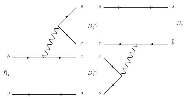
Figure 1: The diagrams of $B_{s}$ and $\bar{B}_{s}$ decay to $D^{(*)}_{s}\bar{D}^{(*)}_{s}$ modes.

We give the first estimation of the contribution to $\Delta\Gamma_{s}$ by three-body $D^{(*)}_{s}\bar{D}^{(*)}\bar{K}^{(*)}$ modes (and their CP conjugates). We use factorization approach, which seems to work well in color-allowed charmful three-body decays Chua:2002pi , in our calculations. As shown in Fig. 2, these modes can be produced by the diagram in Fig. 1, but with an extra $q\bar{q}$ pair produced either in the current or in the spectator part, which we denote as current-produced ($\mathcal{J}$) or transition ($\mathcal{T}$) modes. The number of $D^{(*)}_{s}\bar{D}^{(*)}\bar{K}$ channels are four times larger than $D^{(*)}_{s}\bar{D}^{(*)}_{s}$ modes, with a factor of two coming from extra $q\bar{q}$, which can be $u\bar{u}$ or $d\bar{d}$, and another two from the choice of $q\bar{q}$ in either current or transition processes. With this enhancement in number of modes, and if the branching fractions of these modes are not very small compared with $D^{(*)}_{s}\bar{D}^{(*)}_{s}$ modes, it is natural to expect that $\Delta\Gamma_{s}$ may receive non-negligible contributions from three-body $D^{(*)}_{s}\bar{D}^{(*)}\bar{K}^{(*)}$ modes. So far, the available measurements on these three-body modes are limited to current-produced modes with $\bar{K}$ in $\bar{B}_{u,d}$ systems only Aubert:2003jq ; Aubert:2006fh ; Brodzicka:2007aa ; Aubert:2007rva ; delAmoSanchez:2010pg . These modes are related to the corresponding modes in $\bar{B}_{s}$ system under SU(3) symmetry. We need to reproduce existing three-body data, before we make predictions for the $\bar{B}_{s}$ modes.

Let us briefly survey the experimental situation regarding the SU(3)-related three-body modes. There is no measurement of either transition modes or modes with $\bar{K}^{*}$. Despite a $2.2\sigma$ discrepancy on the branching fraction of $B^{-}\to D^{0}\bar{D}^{0}K^{-}$ decay between measurements  Brodzicka:2007aa ; delAmoSanchez:2010pg , the branching fractions of current-produced $\bar{B}_{u,d}\to D^{(*)}_{u,d}\bar{D}^{(*)}\bar{K}$ modes are around $10^{-2}$ to $10^{-3}$, one order of magnitude smaller compared to two-body modes. So far, $c\bar{s}$ resonances $\bar{D}_{s1}(2536)$ and $\bar{D}_{sJ}(2700)$ have been observed in the decays $\bar{B}_{u,d}\to D^{(*)}_{u,d}\bar{D}^{(*)}\bar{K}$  Aubert:2006fh ; Brodzicka:2007aa ; Aubert:2007rva . For $D_{s1}(2536)$ resonance, its contribution to the branching fractions of three-body decays is in the order of $10^{-4}$, which is small compared with the total branching fraction. On the other hand, Belle observed that $\bar{D}_{sJ}(2700)$ contributes to about half of the total branching fraction of $B^{-}\to D^{0}\bar{D}^{0}K^{-}$. Note that $D_{sJ}(2700)$ has a fairly broad width ($\sim 0.1\,\text{GeV}$). These measurements suggest that $D_{s1}(2536)$ could be treated in a two-body picture while it is more appropriate to consider $D_{sJ}(2700)$ in three-body decays. Furthermore, the contribution of $\bar{D}_{sJ}(2700)$ in $B^{-}\to D^{0}\bar{D}^{0}K^{-}$ decay is $\mathcal{B}(B^{-}\to D^{0}\bar{D}_{sJ}(2700))\times\mathcal{B}(\bar{D}_{sJ}(2700)\to\bar{D}\bar{K})=(0.113^{+0.026}_{-0.040})\%$, which is about half the total branching fraction $(0.222\pm 0.033)\%$  Brodzicka:2007aa . Consequently, the contribution of $\bar{D}_{sJ}(2700)$ in three-body modes and in $\Delta\Gamma_{s}$ should be investigated.

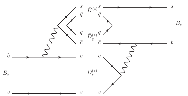
Figure 2: The current and transition diagrams. The left part, $\bar{B}_{s}\to D^{(*)}_{s}\bar{D}^{(*)}\bar{K}^{(*)}$, is the current-produced diagram, and the right part, $B_{s}\to D^{(*)}_{s}\bar{D}^{(*)}\bar{K}^{(*)}$, is transition diagram.

This paper is organized as follows. In Section II, we describe our formalism and briefly review the newly discovered $D_{sJ}(2700)$ resonance that has a non-negligible contribution to three-body modes. The results of two-body modes are in Sec. III.1. For three-body modes, we examine the factorization formalism and calculate $\Delta\Gamma_{s}$ in Sec. III.2. Another scenario and the effect of four-body modes are discussed in Sec. IV, followed by the concluding section. Numerical inputs and some calculational details are collected in three Appendices.

II Formalism

II.1 Formula for $\Delta\Gamma$

The time evolution of a $B_{s}$ meson can be described by the following formula,

$$i\frac{d}{dt}\left({\begin{array}[]{cc}\lvert B\rangle\\ \lvert\bar{B}\rangle\end{array}}\right)=\left(M-i\frac{\Gamma}{2}\right)\left({\begin{array}[]{cc}\lvert B\rangle\\ \lvert\bar{B}\rangle\end{array}}\right),$$ (9)

in which we adopt the phase convention of $\lvert B\rangle$ and $\lvert\bar{B}\rangle$ to be $\textit{CP}\lvert B\rangle=-\lvert\bar{B}\rangle$.  The $\Gamma$ term in Eq. (9) is the absorptive part, which can be calculated by summing all on-shell intermediate states,

$$\Gamma_{ij}=\frac{1}{2M_{B}}\sum_{f}\int d\Phi{\mathcal{A}}^{*}_{B_{i}\to f}(\Phi){\mathcal{A}}_{B_{j}\to f}(\Phi),$$ (10)

where $\Phi$ is over phase space variables. 

We define the width difference $\Delta\Gamma_{s}$ as the difference between light and heavy eigenstates, $\Gamma_{L}-\Gamma_{H}$. Assuming $CP$ conservation, which is a good approximation for SM in $B_{s}-\bar{B}_{s}$ system, the eigenstates of $B_{s}$ meson are $CP$ even and odd states. From short-distance calculation of SM, the light and heavy eigenstates correspond to CP even and odd states respectively. Thus, the $\Delta\Gamma_{s}$ can be related to $\Gamma_{ij}$ by

$$\begin{split}\Delta\Gamma\equiv&\ \Gamma_{L}-\Gamma_{H}\\ =&-2\Gamma_{12}\\ =&-2\times\frac{1}{2M_{B}}\sum_{f}\int d\Phi{\mathcal{A}}^{*}_{B\to f}(\Phi){\mathcal{A}}_{\bar{B}\to f}(\Phi),\end{split}$$ (11)

in which we have used $\Gamma_{21}=\Gamma_{12}^{*}$ from $CPT$ symmetry, and $\Gamma_{12}=\Gamma_{12}^{*}=\text{Re}(\Gamma_{12})$ from $CP$ symmetry. The fact that $\Gamma_{12}$ is real under $CP$ symmetry can be seen from

$$\begin{split}\Gamma_{12}&=\frac{1}{2M_{B}}\sum_{f}\int d\Phi{\mathcal{A}}^{*}_{B\to f}(\Phi){\mathcal{A}}_{\bar{B}\to f}(\Phi)\\ &=\frac{1}{2M_{B}}\sum_{f}\frac{1}{2}\int d\Phi({\mathcal{A}}^{*}_{B\to f}(\Phi){\mathcal{A}}_{\bar{B}\to f}(\Phi)+{\mathcal{A}}^{*}_{B\to\bar{f}}(\Phi){\mathcal{A}}_{\bar{B}\to\bar{f}}(\Phi))\\ &=\frac{1}{2M_{B}}\sum_{f}\text{Re}\left[\int d\Phi{\mathcal{A}}^{*}_{B\to f}(\Phi){\mathcal{A}}_{\bar{B}\to f}(\Phi)\right].\end{split}$$ (12)

The amplitude product ${\mathcal{A}}^{*}_{B\to f}(\Phi){\mathcal{A}}_{\bar{B}\to f}(\Phi)$ is complex conjugate to the amplitude product of conjugate intermediate state ${\mathcal{A}}^{*}_{B\to\bar{f}}(\Phi){\mathcal{A}}_{\bar{B}\to\bar{f}}(\Phi)$ by $CP$ symmetry. $\Gamma_{12}$ sums up all the intermediate states and turns out to be real. For convenience, we define the width difference of each exclusive decay as $\Delta\Gamma_{f}$, and its corresponding complex term in $\Gamma_{12}$ to be

$$\begin{split}\Delta\Gamma_{f}&\equiv-2\times\text{Re}[\Gamma_{12,f}],\end{split}$$ (13)

where $\Gamma_{12,f}$ is defined as

$$\begin{split}\Gamma_{12,f}\equiv\frac{1}{2M_{B}}\int d\Phi{\mathcal{A}}^{*}_{B\to f}(\Phi){\mathcal{A}}_{\bar{B}\to f}(\Phi).\end{split}$$ (14)

Although $\Gamma_{12,f}$ is complex by looking at one mode, the imaginary part is cancelled by its CP conjugate mode, and thus the total $\Gamma_{12}$ turns out to be real. Once ${\mathcal{A}}_{B\to f}(\Phi)$ and ${\mathcal{A}}_{\bar{B}\to f}(\Phi)$ are known, one can readily calculate the corresponding $\Delta\Gamma_{f}$ and branching fractions. In the next section, we will apply the factorization formalism to obtain these amplitudes.

Before we move to model-dependent calculation, it is useful to extract some general limits of the magnitude of $\Delta\Gamma_{f}$ from Eq. (13). For an intermediate state $\lvert f\rangle$, the magnitude of $\Delta\Gamma_{f}$ induced by this state is bounded by

$$\left|\frac{\Delta\Gamma_{f}}{\Gamma}\right|= \ \frac{1}{\Gamma}\cdot\left|\text{Re}[2\Gamma_{12,f}]\right|$$ (15a)

$$\leq \ \frac{1}{\Gamma}\cdot\left|2\Gamma_{12,f}\right|$$ (15b)

$$\leq \ \frac{2}{\Gamma}\cdot\frac{1}{2M_{B}}\int d\Phi\sqrt{|{\mathcal{A}}_{\bar{B}\to f}(\Phi)|^{2}}\sqrt{|{\mathcal{A}}_{B\to f}(\Phi)|^{2}}$$ (15c)

$$\leq \ 2\times\sqrt{{\mathcal{B}}_{\bar{B}\to f}}\times\sqrt{{\mathcal{B}}_{B\to f}}.$$ (15d)

There are three inequalities in this formula. The first inequality reflects that $\Delta\Gamma_{f}$ is only proportional to the real part of $\Gamma_{12,f}$. The second inequality is obtained by the fact that the phase of the amplitude product ${\mathcal{A}}^{*}_{B\to f}(\Phi){\mathcal{A}}_{\bar{B}\to f}(\Phi)$ may be different over the phase space, which would reduce the overall $\lvert\Gamma_{12,f}\rvert$. For the last inequality, it accounts for the “mismatch” effect between $|{\mathcal{A}}_{B\to f}(\Phi)|$ and $|{\mathcal{A}}_{\bar{B}\to f}(\Phi)|$. Even when the branching fractions of $\bar{B}\to f$ and $B\to f$ are the same, the induced $\Delta\Gamma$ could be quite small if the decay probabilities of the two modes are highly mismatched in phase space. Note that the latter two limits are experimental observables. If the branching fractions of $\bar{B}\to f$ and $B\to f$ are measured, one could find the maximal magnitude of the corresponding $\Gamma_{12,f}$. The bound can be refined by the second inequality if the Dalitz plots of the two modes are available. But the $\Delta\Gamma_{f}$, which is proportional to the real part $\Gamma_{12,f}$, could be any value in the range of $-2\lvert\Gamma_{12,f}\rvert$ to $+\lvert 2\Gamma_{12,f}\rvert$.

II.2 Factorization Formalism

The relevant effective Hamiltonian for the $b\to c$ transition is

$${\mathcal{H}_{\rm eff}}=\frac{G_{F}}{\sqrt{2}}V_{cb}V_{cs}^{*}\big{[}c_{1}(\mu)\mathcal{O}^{c}_{1}(\mu)+c_{2}(\mu)\mathcal{O}^{c}_{2}(\mu)\big{]},$$ (16)

where $c_{i}(\mu)$ are the Wilson coefficients, and $V_{cb}$ and $V_{cs}$ are the Cabibbo-Kobayashi-Maskawa (CKM) matrix elements. The four-quark operators ${\mathcal{O}}_{i}$ are products of two $V-A$ currents, i.e. ${\mathcal{O}^{c}_{1}}=(\bar{c}b)_{V-A}\,(\bar{s}c)_{V-A}$ and ${\mathcal{O}^{c}_{2}}=(\bar{s}b)_{V-A}\,(\bar{c}c)_{V-A}$.

With the factorization ansatz, the amplitudes for two-body $\bar{B}_{s}\to\mathcal{D}^{(*)}_{s}\mathcal{\bar{D}}^{(*)}_{s}$ decays are given by

$${\mathcal{A}}(\bar{B}_{s}\to\mathcal{D}^{(*)}_{s}\mathcal{\bar{D}}^{(*)}_{s})=\frac{G_{F}}{\sqrt{2}}V_{cb}V_{cs}^{*}a_{1}\langle\mathcal{D}^{(*)}_{s}|(\bar{c}b)_{V-A}|\bar{B}_{s}\rangle\langle\mathcal{\bar{D}}^{(*)}_{s}|(\bar{s}c)_{V-A}|0\rangle,$$ (17)

where the effective coefficients are expressed as $a_{1}=c_{1}+c_{2}/3$ if naive factorization is used. Note that $\mathcal{D}^{(*)}_{s}$ could be the usual $D^{(*)}_{s}$ and or higher $D_{s}$ resonance such as $D_{s0}^{*}(2317)$, $D_{s1}(2460)$, $D_{s1}(2536)$, and $D_{sJ}(2700)$. The factorized amplitudes consist of the products of two common matrix elements: the current-produced $\mathcal{D}^{(*)}_{s}$ and the $\bar{B}_{s}$ to $\mathcal{D}^{(*)}_{s}$ transition. They are parametrized by the standard way Cheng:2003sm . The matrix elements of current-produced $\mathcal{D}_{s}^{(*)}$ are

$$\begin{split}\langle\mathcal{D}_{s}(p)|(V-A)_{\mu}|0\rangle=&\quad if_{\mathcal{D}_{s}}p_{\mu},\\ \langle\mathcal{D}^{*}_{s}(p,\lambda)|(V-A)_{\mu}|0\rangle=&\quad m_{\mathcal{D}^{*}_{s}}f_{\mathcal{D}^{*}_{s}}\varepsilon^{*}_{\mu}(p,\lambda).\end{split}$$ (18)

The transition matrix elements for $\mathcal{D}_{s}^{(*)}$ are

$$\begin{split}\langle\mathcal{D}_{s}(p_{D})|(V-A)_{\mu}|\bar{B}_{s}(p_{B})\rangle=&\quad\left((p_{B}+p_{D})_{\mu}-\frac{m_{B}^{2}-m_{D}^{2}}{q^{2}}q_{\mu}\right)F_{1}^{\bar{B}_{s}\mathcal{D}_{s}}(q^{2})+\frac{m_{B}^{2}-m_{D}^{2}}{q^{2}}q_{\mu}F_{0}^{\bar{B}_{s}\mathcal{D}_{s}}(q^{2}),\\ \langle\mathcal{D}^{*}_{s}(p_{D^{*}},\lambda)|(V-A)_{\mu}|\bar{B}_{s}(p_{B})\rangle=&\quad\epsilon_{\mu\nu\rho\sigma}\varepsilon^{*\nu}p_{B}^{\rho}p_{D^{*}}^{\sigma}\cdot\frac{2F_{3}^{\bar{B}_{s}\mathcal{D}^{*}_{s}}(q^{2})}{m_{B}+m_{D^{*}}}\\ &-i\left(\varepsilon^{*}_{\mu}-\frac{\varepsilon^{*}\cdot q}{q^{2}}q_{\mu}\right)\,(m_{B}+m_{D^{*}})F_{1}^{\bar{B}_{s}\mathcal{D}^{*}_{s}}(q^{2})\\ &+i\left((p_{B}+p_{D^{*}})_{\mu}-\frac{m_{B}^{2}-m_{D^{*}}^{2}}{q^{2}}q_{\mu}\right)(\varepsilon^{*}\cdot q)\,\frac{F_{2}^{\bar{B}_{s}\mathcal{D}^{*}_{s}}(q^{2})}{m_{B}+m_{D^{*}}}\\ &-i\frac{\varepsilon^{*}\cdot q}{q^{2}}q_{\mu}\,2m_{D^{*}}F_{0}^{\bar{B}_{s}\mathcal{D}^{*}_{s}}(q^{2}),\end{split}$$ (19)

where $\epsilon_{\mu\nu\rho\sigma}$ is the totally anti-symmetric symbol with $\epsilon_{0123}=1$. For convenience, our notations of decay constants and form factors of $D^{**}_{s}$ are different from the usual notations. The conversion can be found in Appendix B.

The amplitudes of three-body modes $D^{(*)}\bar{D}^{(*)}\bar{K}^{(*)}$ decayed from $\bar{B}$ and $B$ are given by

$$\begin{split}{\mathcal{A}_{\mathcal{J}}}(\bar{B}_{s}\to D_{s}^{(*)}\bar{D}^{(*)}\bar{K}^{(*)})&=\frac{G_{F}}{\sqrt{2}}V_{cb}V_{cs}^{*}a_{1}\langle D_{s}^{(*)}|(\bar{c}b)_{V-A}|\bar{B}_{s}\rangle\cdot\langle\bar{D}^{(*)}\bar{K}^{(*)}|(\bar{s}c)_{V-A}|0\rangle,\\ {\mathcal{A}_{\mathcal{T}}}(B_{s}\to D_{s}^{(*)}\bar{D}^{(*)}\bar{K}^{(*)})&=\frac{G_{F}}{\sqrt{2}}V_{cb}V_{cs}^{*}a_{1}\langle\bar{D}^{(*)}\bar{K}^{(*)}|(\bar{c}b)_{V-A}|B_{s}\rangle\cdot\langle D_{s}^{(*)}|(\bar{s}c)_{V-A}|0\rangle,\end{split}$$ (20)

where $\mathcal{A}_{\mathcal{J}}$ and $\mathcal{A}_{\mathcal{T}}$ denote the amplitudes of current and transition diagrams, respectively. Unlike the $\mathcal{D}^{(*)}_{s}\mathcal{\bar{D}}^{(*)}_{s}$ modes in which only standard form factors appear, these amplitudes involve the time-like form factors and transition form factors of two pseudoscalars ($\bar{D}\bar{K}$) or vectors ($\bar{D}^{*}\bar{K}^{*}$), or a pseudoscalar with a vector ($\bar{D}^{*}\bar{K}$ or $\bar{D}\bar{K}^{*}$).

The parametrization of time-like form factors are similar to the space-like counterparts, such as $\langle D_{s}^{(*)}|V-A|\bar{B}_{s}\rangle$. The time-like form factors of two pseudoscalars ($PP$) states are given by

$$\begin{split}\langle P_{a}(p_{a})P_{b}(p_{b})|(V-A)_{\mu}|0\rangle=&\left((p_{a}-p_{b})_{\mu}-\frac{m_{a}^{2}-m_{b}^{2}}{q^{2}}q_{\mu}\right)F_{1}^{PP}(q^{2})+\frac{m_{a}^{2}-m_{b}^{2}}{q^{2}}q_{\mu}F_{0}^{PP}(q^{2}),\end{split}$$ (21)

where $q^{\mu}=p_{a}^{\mu}+p_{b}^{\mu}$ is the momentum of the current. For the states with one vector and pseudoscalar ($VP$), the parametrization of time-like form factors are

$$\begin{split}\langle V(p_{V},\varepsilon_{V})P(p_{P})|(V-A)_{\mu}|0\rangle=&-\epsilon_{\mu\nu\rho\sigma}\varepsilon_{V}^{*\nu}p_{P}^{\rho}p_{V}^{\sigma}\cdot\frac{2V^{VP}(q^{2})}{m_{V}+m_{P}}-i\left(\varepsilon^{*}_{V\mu}-\frac{\varepsilon_{V}^{*}\cdot q}{q^{2}}q_{\mu}\right)(m_{V}+m_{P})A_{1}^{VP}(q^{2})\\ &-i\left((p_{V}-p_{P})_{\mu}-\frac{m_{V}^{2}-m_{P}^{2}}{q^{2}}q_{\mu}\right)(\varepsilon_{V}^{*}\cdot q)\,\frac{A_{2}^{VP}(q^{2})}{m_{V}+m_{P}}-i\frac{\varepsilon_{V}^{*}\cdot q}{q^{2}}q_{\mu}\,2m_{V}A_{0}^{VP}(q^{2}).\end{split}$$ (22)

The time-like form factors of two vectors ($VV$) states can be parameterized analogously,

$$\begin{split}\langle V_{a}(p_{a},\varepsilon_{a})V_{b}(p_{b},\varepsilon_{b})|(V-A)_{\mu}|0\rangle=&\quad i\epsilon_{\alpha\nu\rho\sigma}\varepsilon_{b}^{*\alpha}\varepsilon_{a}^{*\nu}p_{a}^{\rho}p_{b}^{\sigma}q_{\mu}\frac{V^{VV}_{0}(q^{2})}{(m_{a}+m_{b})^{2}}+i\epsilon_{\mu\nu\rho\sigma}\varepsilon_{a}^{*\nu}p_{a}^{\rho}p_{b}^{\sigma}(\varepsilon_{b}^{*}\cdot q)\frac{V^{VV}_{1}(q^{2})}{(m_{a}+m_{b})^{2}}\\ &+i\epsilon_{\mu\nu\rho\sigma}\varepsilon_{b}^{*\nu}p_{a}^{\rho}p_{b}^{\sigma}(\varepsilon_{a}^{*}\cdot q)\frac{V^{VV}_{2}(q^{2})}{(m_{a}+m_{b})^{2}}+\left(\varepsilon^{*}_{a\mu}-\frac{\varepsilon_{a}^{*}q}{q^{2}}q_{\mu}\right)(\varepsilon_{b}^{*}\cdot q)A_{11}^{VV}(q^{2})\\ &+\left(\varepsilon^{*}_{b\mu}-\frac{\varepsilon_{b}^{*}\cdot q}{q^{2}}q_{\mu}\right)(\varepsilon_{a}^{*}\cdot q)A_{12}^{VV}(q^{2})+\left((p_{a}-p_{b})_{\mu}-\frac{m_{a}^{2}-m_{b}^{2}}{q^{2}}q_{\mu}\right)(\varepsilon_{a}^{*}\cdot\varepsilon_{b}^{*})A_{2}^{VV}(q^{2})\\ &+(\varepsilon_{a}^{*}\cdot q)(\varepsilon_{b}^{*}\cdot q)\frac{q_{\mu}}{q^{2}}A_{01}^{VV}(q^{2}),+(\varepsilon_{a}^{*}\cdot\varepsilon_{b}^{*})\frac{q_{\mu}}{q^{2}}(m_{a}+m_{b})^{2}A_{02}^{VV}(q^{2}).\end{split}$$ (23)

The transition form factors are more complicated. The case of $B_{s}$ to $PP$ transition form factors were formulated in a general way in Ref. Lee:ih , which can be rewritten as

$$\begin{split}\langle P_{a}(p_{a})P_{b}(p_{b})|(V-A)_{\mu}|\bar{B}_{s}(p_{B})\rangle=&\quad\epsilon_{\mu\nu\rho\sigma}p_{B}^{\nu}q^{\rho}(p_{a}-p_{b})^{\sigma}\,\frac{V^{\bar{B}_{s}PP}}{m_{B_{s}}^{3}}+i\left((p_{B}+q)_{\mu}-\frac{m_{B_{s}}^{2}-q^{2}}{q^{\prime 2}}q^{\prime}_{\mu}\right)\,\frac{A_{1}^{\bar{B}_{s}PP}}{m_{B_{s}}}\\ &+i\left((p_{a}-p_{b})_{\mu}-\frac{m_{a}^{2}-m_{b}^{2}}{q^{2}}q_{\mu}\right)\,\frac{A_{2}^{\bar{B}_{s}PP}}{m_{B_{s}}}+i\frac{m_{a}^{2}-m_{b}^{2}}{q^{2}}q_{\mu}\,\frac{A_{0}^{\bar{B}_{s}PP}}{m_{B_{s}}},\end{split}$$ (24)

where $q^{\mu}=p_{a}^{\mu}+p_{b}^{\mu}$ is the total momentum of $PP$, and $q^{\prime\mu}=p_{B}^{\mu}-q^{\mu}$ is the momentum of the external current. In this form, the terms with $A_{1}$ and $A_{2}$ are zeros when contracted with $q^{\prime}$ and $q$. For the transition form factors of $\bar{B}_{s}$ to $VP$ and $VV$, since they are more complicated and there is so far no data, we only write down the form factors obtained from pole model rather than the general forms. For $VP$, we have

$$\begin{split}\langle V(p_{V},\varepsilon_{V})P(p_{P})|(V-A)^{\mu}|\bar{B}_{s}(p_{B})\rangle=&\quad i\epsilon_{\alpha\nu\rho\sigma}\left(-g^{\mu\alpha}+\frac{q^{\prime\mu}q^{\prime\alpha}}{q^{\prime 2}}\right)\varepsilon_{V}^{*\nu}p_{P}^{\rho}p_{V}^{\sigma}\,\frac{V^{\bar{B}_{s}VP}_{2}}{m_{B_{s}}^{2}}\\ &+i\epsilon_{\alpha\nu\rho\sigma}q^{\prime\alpha}\varepsilon_{V}^{*\nu}p_{P}^{\rho}p_{V}^{\sigma}\left((p_{B}+q)^{\mu}-\frac{m_{B_{s}}^{2}-q^{2}}{q^{\prime 2}}q^{\prime\mu}\right)\,\frac{V^{\bar{B}_{s}VP}_{1}}{m_{B_{s}}^{4}}\\ &+i\epsilon_{\alpha\nu\rho\sigma}q^{\prime\alpha}\varepsilon_{V}^{*\nu}p_{P}^{\rho}p_{V}^{\sigma}\frac{q^{\prime\mu}}{q^{\prime 2}}\,\frac{V^{\bar{B}_{s}VP}_{0}}{m_{B_{s}}^{2}}\\ &+\epsilon_{\alpha\beta\gamma\delta}\epsilon_{abcd}(g^{\mu\alpha}g^{\beta a})q^{\prime\gamma}q^{\delta}\varepsilon_{V}^{*b}p_{P}^{c}p_{V}^{d}\,\frac{A^{\bar{B}_{s}VP}_{3}}{m_{B_{s}}^{4}}\\ &+\left((p_{B}+q)^{\mu}-\frac{m_{B_{s}}^{2}-q^{2}}{q^{\prime 2}}q^{\prime\mu}\right)(\varepsilon_{V}^{*}\cdot q)\,\frac{A_{1}^{\bar{B}_{s}VP}}{m_{B_{s}}^{2}}+\frac{m_{B_{s}}^{2}-q^{2}}{q^{\prime 2}}q^{\prime\mu}(\varepsilon_{V}^{*}\cdot q)\,\frac{A_{0}^{\bar{B}_{s}VP}}{m_{B_{s}}^{2}},\end{split}$$ (25)

and for $\bar{B}_{s}$ to $VV$, we parameterize as

$$\begin{split}&\langle V_{a}(p_{a},\varepsilon_{a})V_{b}(p_{b})|(V-A)_{\mu}|\bar{B}_{s}(p_{B})\rangle\\ &\ \ \ \ \ \ \ \ \ \ \ \ \ =\epsilon_{\mu\nu\rho\sigma}p_{a}^{\nu}p_{b}^{\rho}q^{\prime\sigma}(\varepsilon_{a}^{*}\cdot\varepsilon_{b}^{*})\,\frac{V^{\bar{B}_{s}VV}_{3}}{m_{B_{s}}^{3}}+\epsilon_{\mu\nu\rho\sigma}\varepsilon_{a}^{*\nu}q^{\prime\rho}q^{\sigma}(\varepsilon_{b}^{*}\cdot q)\,\frac{V^{\bar{B}_{s}VV}_{2}}{m_{B_{s}}^{3}}\\ &\ \ \ \ \ \ \ \ \ \ \ \ \ \ \ +\epsilon_{\mu\nu\rho\sigma}\varepsilon_{b}^{*\nu}q^{\prime\rho}q^{\sigma}(\varepsilon_{a}^{*}\cdot q)\,\frac{V^{\bar{B}_{s}VV}_{1}}{m_{B_{s}}^{3}}+\epsilon_{\alpha\nu\rho\sigma}\varepsilon_{b}^{*\alpha}\varepsilon_{a}^{*\nu}p_{a}^{\rho}p_{b}^{\sigma}\left((p_{B}+q)_{\mu}-\frac{m_{B_{s}}^{2}-q^{2}}{q^{\prime 2}}q^{\prime}_{\mu}\right)\,\frac{V^{\bar{B}_{s}VV}_{01}}{m_{B_{s}}^{3}}\\ &\ \ \ \ \ \ \ \ \ \ \ \ \ \ \ +\epsilon_{\alpha\nu\rho\sigma}\varepsilon_{b}^{*\alpha}\varepsilon_{a}^{*\nu}p_{a}^{\rho}p_{b}^{\sigma}\frac{m_{B_{s}}^{2}-q^{2}}{q^{\prime 2}}q^{\prime}_{\mu}\,\frac{V^{\bar{B}_{s}VV}_{00}}{m_{B_{s}}^{3}}\\ &\ \ \ \ \ \ \ \ \ \ \ \ \ \ \ +i(\varepsilon_{a}^{*}\cdot\varepsilon_{b}^{*})\left((p_{a}-p_{b})_{\mu}-\frac{m_{a}^{2}-m_{b}^{2}}{q^{\prime 2}}q^{\prime}_{\mu}\right)\,\frac{A_{62}^{\bar{B}_{s}VV}}{m_{B_{s}}}\\ &\ \ \ \ \ \ \ \ \ \ \ \ \ \ \ +i(\varepsilon_{a}^{*}\cdot\varepsilon_{b}^{*})\left((p_{B}+q)_{\mu}-\frac{m_{B_{s}}^{2}-q^{2}}{q^{\prime 2}}q^{\prime}_{\mu}\right)\,\frac{A_{61}^{\bar{B}_{s}VV}}{m_{B_{s}}}+i(\varepsilon_{a}^{*}\cdot\varepsilon_{b}^{*})\frac{q^{\prime}_{\mu}}{q^{\prime 2}}\,m_{B_{s}}A_{60}^{\bar{B}_{s}VV}\\ &\ \ \ \ \ \ \ \ \ \ \ \ \ \ \ +i(\varepsilon_{b}^{*}\cdot q)\left(\varepsilon^{*}_{a\mu}-\frac{\varepsilon_{a}^{*}q}{q^{2}}q_{\mu}\right)\,\frac{A_{3}^{\bar{B}_{s}VV}}{m_{B_{s}}}+i(\varepsilon_{a}^{*}\cdot q)\left(\varepsilon^{*}_{b\mu}-\frac{\varepsilon_{b}^{*}q}{q^{2}}q_{\mu}\right)\,\frac{A_{4}^{\bar{B}_{s}VV}}{m_{B_{s}}}\\ &\ \ \ \ \ \ \ \ \ \ \ \ \ \ \ +i(\varepsilon_{a}^{*}\cdot q^{\prime})(\varepsilon_{b}^{*}\cdot q)\left((p_{B}+q)_{\mu}-\frac{m_{B_{s}}^{2}-q^{2}}{q^{\prime 2}}q^{\prime}_{\mu}\right)\,\frac{A_{21}^{\bar{B}_{s}VV}}{m_{B_{s}}^{3}}+i(\varepsilon_{a}^{*}\cdot q^{\prime})(\varepsilon_{b}^{*}\cdot q)\frac{q^{\prime}_{\mu}}{q^{\prime 2}}\,\frac{A_{20}^{\bar{B}_{s}VV}}{m_{B_{s}}}\\ &\ \ \ \ \ \ \ \ \ \ \ \ \ \ \ +i(\varepsilon_{a}^{*}\cdot q)(\varepsilon_{b}^{*}\cdot q^{\prime})\left((p_{B}+q)_{\mu}-\frac{m_{B_{s}}^{2}-q^{2}}{q^{\prime 2}}q^{\prime}_{\mu}\right)\,\frac{A_{11}^{\bar{B}_{s}VV}}{m_{B_{s}}^{3}}+i(\varepsilon_{a}^{*}\cdot q)(\varepsilon_{b}^{*}\cdot q^{\prime})(\frac{q^{\prime}_{\mu}}{q^{\prime 2}})\,\frac{A_{10}^{\bar{B}_{s}VV}}{m_{B_{s}}}\\ &\ \ \ \ \ \ \ \ \ \ \ \ \ \ \ +i(\varepsilon_{a}^{*}\cdot q)(\varepsilon_{b}^{*}\cdot q)\left((p_{B}+q)_{\mu}-\frac{m_{B_{s}}^{2}-q^{2}}{q^{\prime 2}}q^{\prime}_{\mu}\right)\,\frac{A_{01}^{\bar{B}_{s}VV}}{m_{B_{s}}^{3}}+i(\varepsilon_{a}^{*}\cdot q)(\varepsilon_{b}^{*}\cdot q)\frac{q^{\prime}_{\mu}}{q^{\prime 2}}\,\frac{A_{00}^{\bar{B}_{s}VV}}{m_{B_{s}}}.\\ \end{split}$$ (26)

Under CP conservation, all these form factors can be related to the form factors of their CP conjugates. These transformations are provided in Appendix B.

II.3 Pole Model

Figure 3: Pole diagram of $\bar{B}_{s}-B_{s}$ mixing. Left: current-produced diagram. Right: transition diagram.

Since the branching fractions of $D^{(*)}_{s}\bar{D}^{(*)}_{s}$ are large, it is natural to expect a sizable contribution from off-shell $D^{(*)}_{s}$ poles. In addition, experiments have observed $D_{sJ}(2700)$ in the three-body decays as we have described in the introduction  Aubert:2006fh ; Brodzicka:2007aa . $D_{sJ}(2700)$ can decay to on-shell $D^{(*)}K$, but only goes off-shell to $D^{(*)}K^{*}$ because of kinematics. As shown in Fig. 3, we consider pole exchanges, including $D_{s}$, $D^{*}_{s}$ and $D_{sJ}(2700)$, in three-body decays. Note that the $D_{s}$ pole only goes to $D^{*}K$ rather than $DK$.

In the following calculation, we use off-shell $D^{(*)}_{s}$ poles and $D_{sJ}(2700)$ to model the $D^{(*)}K^{(*)}$ form factors. The effective Lagrangian taken from Ref. Casalbuoni:1996pg ; Yan:1992gz ; Cheng:2004ru is applied to describe the interaction between $D^{(*)}_{q}$ mesons and light psedudoscalar or vector mesons. The pole contribution to $D^{(*)}K^{(*)}$ form factors can be calculated by

$$\begin{split}\langle D^{(*)}K^{(*)}|(V-A)_{\mu}|0\rangle_{\rm pole}=&\frac{i}{q^{2}-m_{\rm int}^{2}+im_{\rm int}\Gamma_{\rm int}}\times\langle D^{(*)}K^{(*)}|i\mathcal{L}_{\rm eff}|D_{\rm int}\rangle\langle D_{\rm int}|(V-A)_{\mu}|0\rangle\\ &+\frac{i}{q^{2}-m_{\rm int*}^{2}+im_{\rm int*}\Gamma_{\rm int*}}\times\left(-g^{\alpha\beta}+\frac{q^{\alpha}q^{\beta}}{m^{2}_{\rm int*}}\right)\\ &\times\frac{\partial^{2}}{\partial\varepsilon_{\rm int}^{*\alpha}\partial\varepsilon_{\rm int}^{\beta}}\left(\langle D^{(*)}K^{(*)}|i\mathcal{L}_{\rm eff}|D^{*}_{\rm int}\rangle\langle D^{*}_{\rm int}|(V-A)_{\mu}|0\rangle\right),\\ \langle D^{(*)}K^{(*)}|(V-A)_{\mu}|\bar{B}\rangle_{\rm pole}=&\frac{i}{q^{2}-m_{\rm int}^{2}+im_{\rm int}\Gamma_{\rm\rm int}}\times\langle D^{(*)}K^{(*)}|i\mathcal{L}_{\rm eff}|D_{\rm int}\rangle\langle D_{int}|(V-A)_{\mu}|\bar{B}\rangle\\ &+\frac{i}{q^{2}-m_{\rm int*}^{2}+im_{\rm int*}\Gamma_{\rm\rm int*}}\times\left(-g^{\alpha\beta}+\frac{q^{\alpha}q^{\beta}}{m^{2}_{\rm int*}}\right)\\ &\times\frac{\partial^{2}}{\partial\varepsilon_{\rm int}^{*\alpha}\partial\varepsilon_{\rm int}^{\beta}}\left(\langle D^{(*)}K^{(*)}|i\mathcal{L}_{\rm eff}|D^{*}_{\rm int}\rangle\langle D^{*}_{int}|(V-A)_{\mu}|\bar{B}\rangle\right),\end{split}$$ (27)

where the $D^{(*)}_{\rm int}$ is the intermediate particle with mass $m_{\rm int(*)}$ and width $\Gamma_{\rm int(*)}$. We adopt the Breit-Wigner form of the propagator and replace $\varepsilon_{\rm int}^{*\alpha}\varepsilon_{\rm int}^{\beta}$ as $(-g^{\alpha\beta}+{q^{\alpha}q^{\beta}}/{m^{2}_{\rm int*}})$ to account for the off-shell effect. The explicit forms of the matrix elements $\langle D^{(*)}K^{(*)}|i\mathcal{L}_{\rm eff}|D^{(*)}_{\rm int}\rangle$ in the above equations can be found in Ref. Cheng:2004ru . A full list of pole contribution to form factors are listed in Appendix C.

II.4 $D_{sJ}(2700)$ Resonance

The relevant properties and parameters of $D_{sJ}(2700)$ are summarized in this section. The mass and width of this resonance are PDG

$$\begin{split}m_{D_{sJ}(2700)}&=2709^{+9}_{-6}\text{ MeV},\\ \Gamma_{D_{sJ}(2700)}&=125\pm 30\text{ MeV}.\end{split}$$ (28)

Note that the width has a large uncertainty ($\sim 25\%$). The ratio of branching fractions of this resonance to $DK$ and $D^{*}K$ is also measured Aubert:2009di

$$\begin{split}r(D^{*}K)\equiv\frac{\mathcal{B}(D_{sJ}(2700)^{+}\to D^{*}K)}{\mathcal{B}(D_{sJ}(2700)^{+}\to DK)}&=0.91\pm 0.13_{\rm stat}\pm 0.12_{\rm syst},\end{split}$$ (29)

where $D^{(*)}K$ is the average of $D^{(*)}K_{S}$ and $D^{(*)}K^{+}$ modes. On the other hand, the contribution of $D_{sJ}(2700)$ in the decay $B^{+}\to\bar{D}^{0}D^{0}K^{+}$, denoted as $\mathcal{B}(B^{+}\to\bar{D}^{0}D_{sJ}(2700))\times\mathcal{B}(D_{sJ}(2700)\to D^{0}K^{+})$, is extracted Brodzicka:2007aa

$$\begin{split}\mathcal{B}(B^{+}\to\bar{D}^{0}D_{sJ}(2700))\times\mathcal{B}(D_{sJ}(2700)\to DK)=(11.3^{+2.6}_{-4.0})\times 10^{-4},\end{split}$$ (30)

which constitutes about half the total branching fraction of this measurement. Note that this quantity has a large uncertainty, similar to the measurement of width. The quantum number of $D_{sJ}(2700)$ is determined to be $J^{P}=1^{-}$ from helicity angle distribution, which limits this resonance to be either an $s$-wave or $d$-wave meson (or a mixed state between them). The interpretation of $D_{sJ}(2700)$ as a radial excitation of $D^{*}_{s}$ ($n^{2S+1}L_{J}=2^{3}S_{1}$) is proposed, which can explain its mass Godfrey:1985xj , partial width Colangelo:2007ds , and contribution in $B^{+}\to\bar{D}^{0}D^{0}K^{+}$ decay Wang:2009zz . In some strong decay models, a mixed state $2^{3}S_{1}-1^{3}D_{1}$ describes the partial width better Close:2006gr . As the theoretical predictions of mass and partial width are highly model-dependent, the identification is still not clear yet. We assume $D_{sJ}(2700)$ as a $2^{3}S_{1}$ state in this study.

The effective Lagrangian in Ref. Casalbuoni:1996pg ; Yan:1992gz ; Cheng:2004ru can still be applied to describe the interaction between $D_{sJ}(2700)$ and light mesons Colangelo:2007ds . We work out the relevant matrix elements,

$$\begin{split}\langle D(p_{2})K(p_{3})|i\mathcal{L}_{\rm eff}|D_{sJ}(2700)(p_{1},\varepsilon_{1})\rangle=&-i\tilde{g}_{D_{sJ}DK}\,\varepsilon_{1}\cdot p_{3},\\ \langle D^{*}(p_{2},\varepsilon_{2})K(p_{3})|i\mathcal{L}_{\rm eff}|D_{sJ}(2700)(p_{1},\varepsilon_{1})\rangle=&-i\tilde{g}_{D_{sJ}D^{*}K}\,\epsilon_{\mu\nu\alpha\beta}\varepsilon_{1}^{\mu}\varepsilon_{2}^{\nu}p_{3}^{\alpha}p_{1}^{\beta},\end{split}$$ (31)

where the strong coupling constants are given by Ref. Colangelo:2007ds ,

$$\begin{split}\tilde{g}_{D_{sJ}DK}&=2\frac{\tilde{g}}{f_{\pi}}\sqrt{m_{D_{sJ}}m_{D}},\\ \tilde{g}_{D_{sJ}D^{*}K}&=2\frac{\tilde{g}}{f_{\pi}}\sqrt{\frac{m_{D^{*}}}{m_{D_{sJ}}}},\end{split}$$ (32)

with $f_{\pi}=132\ \text{MeV}$. Once the coupling constants and form factors are extracted, one can insert Eq. (31) into Eq. (27) to obtained the contribution to form factors from the $D_{sJ}(2700)$ resonance.

From these matrix elements, Ref. Colangelo:2007ds predicted the ratio of branching fractions

$$\begin{split}r(D^{*}K)=0.91\pm 0.04.\end{split}$$ (33)

This ratio agrees with Eq. (29) very well. The ratios of the branching fractions of the six main decay modes are given by Table 1. The mixing angle between $\eta$ and $\eta^{\prime}$ is taken from Ref. Feldmann:1998sh .

Mode(f)	$D^{0}K^{+}$	$D^{+}\bar{K}^{0}$	$D^{*0}K^{+}$	$D^{*+}\bar{K}^{0}$	$D_{s}\eta$	$D^{*}_{s}\eta$
$r(f)$	1.02	0.98	0.93	0.89	0.17	0.04

Table 1: The ratio $r$ of the branching fractions of six main decay modes of the $D_{sJ}(2700)^{+}$ resonance.

Assuming $D_{sJ}(2700)$ only decays to $D^{(*)}K$ and $D^{(*)}\eta^{(\prime)}$, $\tilde{g}^{2}$ is proportional to the total width. Thus, we have

$$\tilde{g}=0.28\pm 0.03,$$ (34)

where the uncertainty comes from the uncertainty of the total width. Note that this value is slightly larger than the one in Ref. Colangelo:2007ds as the world-average of width [Eq. (28)] became larger.

Taking the measured mass, width and $\mathcal{B}(B\to\bar{D}^{(*)}D_{sJ}(2700))\times\mathcal{B}(D_{sJ}(2700)\to DK)$ (see Sec. III. B for details) as input, the $D_{sJ}(2710)$ decay constant is extracted as

$$f_{D_{sJ}(2700)}=240\pm 31\text{ MeV}.$$ (35)

The decay constant can be compared to the previous estimations $243\pm 41~{}\text{MeV}$ in Ref. Colangelo:2007ds and $295\pm 13~{}\text{MeV}$ in Ref. Wang:2009zz . Note that it is compatible to the decay constants of $D^{(*)}_{s}$, which we use $260\pm 13~{}\text{MeV}$ in later calculation.

The $\bar{B}_{s}\to D_{sJ}(2700)$ transition form factors can be obtained by using a covariant light-front quark model Cheng:2004ru . For the $2S$ wave function,  its Gaussian width can be fixed by the decay constant derived from Eq. (30). It is then straightforward to obtain various $\bar{B}_{s}\to D_{sJ}$ form factors:

$$\begin{split}V^{\bar{B}_{s}D_{sJ}(2700)}(q^{2})&=\frac{0.25\pm 0.03}{1-0.03\,q^{2}/m_{Bs}^{2}+0.38\,q^{4}/m_{Bs}^{4}},\\ A^{\bar{B}_{s}D_{sJ}(2700)}_{0}(q^{2})&=\frac{0.24\pm 0.02}{1+1.16\,q^{2}/m_{Bs}^{2}+2.16\,q^{4}/m_{Bs}^{4}},\\ A^{\bar{B}_{s}D_{sJ}(2700)}_{1}(q^{2})&=\frac{0.17\pm 0.02}{1+0.66\,q^{2}/m_{Bs}^{2}+0.54\,q^{4}/m_{Bs}^{4}},\\ A^{\bar{B}_{s}D_{sJ}(2700)}_{2}(q^{2})&=\frac{0.007\pm 0.001}{1+4.84\,q^{2}/m_{Bs}^{2}+5.08\,q^{4}/m_{Bs}^{4}}.\\ \end{split}$$ (36)

These transition form factors are small comparing to the $D^{(*)}_{s}$ (collected in Appendix A), because of the poor overlap between wave functions of ground state $B$ mesons and the radial excited $D_{sJ}(2700)$.

II.5 Non-Resonance Contribution

In general, there will be both resonant and non-resonant (NR) contributions to form factors. In previous study of $\bar{B}\to D^{(*)}K^{-}K^{0}$ decays Chua:2002pi , it is necessary to add NR contribution to form factors to explain the experimental observations. Therefore, we should include the NR effect in this work. To produce the $D^{(*)}K^{(*)}$ pairs, at least one gluon must be emitted to produce $q\bar{q}$ pairs. The QCD counting rule Chua:2002pi provides an ansatz for the asymptotic behavior of the non-resonant form factors, which is

$$F(q^{2})_{NR}\rightarrow\frac{x_{F}}{q^{2}}\left[\text{ln}\left(\frac{q^{2}}{\Lambda^{2}}\right)\right]^{-1},$$ (37)

where $q^{2}$ is the invariant mass of $D^{(*)}K^{(*)}$ and $\Lambda=0.5\text{ GeV}$ is the QCD scale.

Together with the pole contribution provided in Appendix C, the complete form factors are modeled by the pole and NR contribution,

$$F(q^{2})=F(q^{2})|_{\rm pole}+\frac{x_{F}}{q^{2}}\left[\text{ln}\left(\frac{q^{2}}{\Lambda^{2}}\right)\right]^{-1},$$ (38)

where the asymptotic form of NR contribution is adopted for simplicity. As more data is available in the future, one could replace this simple form with a more sophisticated one to fit the data, as in Ref. Chua:2002pi .

III Results

III.1 Two-body $\mathcal{D}^{(*)}_{s}\mathcal{\bar{D}}^{(*)}_{s}$ Decays and the Width Difference: An Update

We first update the branching fractions of two-body $\bar{B}_{s}\to D^{(*)}_{s}\bar{D}^{(*)}_{s}$ decays, which contribute to $\Delta\Gamma_{s}$. The necessary parameters are given in Appendix A. Our results are listed in Table 2, where experimental results and previous theoretical results from Ref. Aleksan:1993qp are listed for comparison. Since SU(3)-related modes in $B_{u,d}$ systems are usually more precisely known than the $B_{s}$ system, we also list them in parentheses for comparison. For example, data for $\mathcal{B}(\bar{B}_{u}\to D_{u}\bar{D}_{s})$, which is approximately the same as $\mathcal{B}(\bar{B}_{s}\to D_{s}\bar{D}_{s})$ under SU(3) limit, is listed. Note that two uncertainties are given in our results: The first uncertainty is obtained by varying decay constants and form factors by 5%, while the second comes from the estimated $10\%$ uncertainty in $a_{1}$.

Mode(f)	$\mathcal{B}(\bar{B}_{s,(u)}\to f)$ (%) data	$\mathcal{B}(\bar{B}_{s}\to f)$ (%) this work	$\mathcal{B}(\bar{B}_{s}\to f)$ (%) Ref. Aleksan:1993qp	$\Delta\Gamma_{f}/\Gamma_{s}$ (%) this work	$\Delta\Gamma_{f}/\Gamma_{s}$ (%) Ref. Aleksan:1993qp
$D_{s}\bar{D}_{s}$	$1.04\pm 0.35$  ($1.00\pm 0.17$)	$1.4\pm 0.3\pm 0.3$	1.6	$2.7\pm 0.6\pm 0.6$	3.1
$D_{s}^{*}\bar{D}_{s}$+$D_{s}\bar{D}_{s}^{*}$	$2.75\pm 1.08$  ($1.58\pm 0.33$)	$1.8\pm 0.4\pm 0.4$	2.2	$3.6\pm 0.8\pm 0.8$	4.4
$D_{s}^{*}\bar{D}_{s}^{*}$	$3.08\pm 1.49$  ($1.71\pm 0.24$)	$2.3\pm 0.5\pm 0.5$	3.6	$3.8\pm 0.8\pm 0.8$	6.9
$D_{s}^{(*)}\bar{D}_{s}^{(*)}$	$4.9\pm 1.4$  $6.9\pm 2.3$  $4.0\pm 1.5$  ($4.29\pm 0.74$)	$5.5\pm 1.2\pm 1.1$	7.4	$10.2\pm 2.2\pm 2.1$	14.4

Table 2: The branching fractions of $\bar{B}_{s}\to D^{(*)}_{s}\bar{D}^{(*)}_{s}$ decays and their contribution to the width difference. The results can be compared with data in Refs. PDG ; Esen:2010jq ; HFAG:2010 . The data for $B^{-}$ system in Ref. PDG , which are related to $B_{s}$ under SU(3) symmetry, are shown in parentheses (see text for detail). The theoretical result of Ref. Aleksan:1993qp is also presented for comparison.

The branching fractions of $D_{s}^{(*)}\bar{D}_{s}^{(*)}$ modes are all of percent level. In general, our result is smaller than the result in Ref. Aleksan:1993qp . These branching fractions can be compared with experimental data in both $B_{s}$ and $B^{-}$ system. One can see that our results agree with experiment within uncertainties. The direct measurement of $\bar{B}_{s}\to D_{s}^{(*)}\bar{D}_{s}^{(*)}$ exclusive decays was recently reported by Belle Esen:2010jq .  While the observed branching fraction of $D_{s}\bar{D}_{s}$ mode $(1.0\pm 0.4)\%$ is close to our result, other modes are more aligned with the calculation in Ref. Aleksan:1993qp . But the world average of the inclusive branching fraction $\mathcal{B}(\bar{B}_{s}\to D_{s}^{(*)}\bar{D}_{s}^{(*)})$  HFAG:2010 ; PDG and the rates of SU(3) related modes are closer to our results.

Mode(f)	$\mathcal{B}(\bar{B}_{s}\to f)$ (%)	$\mathcal{B}(B_{s}\to f)$ (%)	$\Delta\Gamma_{f}/\Gamma_{s}$ (%)
$D_{s}\bar{D}_{s0}^{*}(2317)$	$0.10\pm 0.02\pm 0.02$ ($0.073^{+0.022}_{-0.017}$)	$0.15\pm 0.03\pm 0.03$	$-0.24\pm 0.05\pm 0.05$
$D^{*}_{s}\bar{D}_{s0}^{*}(2317)$	$0.05\pm 0.01\pm 0.01$ ($0.09\pm 0.07$)	$0.12\pm 0.03\pm 0.03$	$-0.15\pm 0.03\pm 0.03$
$D_{s}\bar{D}_{s1}(2460)$	$0.24\pm 0.05\pm 0.05$ ($0.31^{+0.10}_{-0.09}$)	$0.04\pm 0.01\pm 0.01$	$-0.18\pm 0.04\pm 0.04$
$D^{*}_{s}\bar{D}_{s1}(2460)$	$0.81\pm 0.17\pm 0.17$ ($1.20\pm 0.30$)	$0.06\pm 0.01\pm 0.01$	$+0.16\pm 0.03\pm 0.03$
$D_{s}\bar{D}_{s1}(2536)$	$0.02\pm 0.01\pm 0.01$ ($0.022\pm 0.007$)	$0.38\pm 0.08\pm 0.08$	$+0.19\pm 0.04\pm 0.04$
$D^{*}_{s}\bar{D}_{s1}(2536)$	$0.09\pm 0.02\pm 0.02$ ($0.055\pm 0.0016$)	$0.38\pm 0.08\pm 0.08$	$+0.34\pm 0.07\pm 0.07$
$D_{s0}^{*}(2317)\bar{D}_{s1}(2460)$	$0.024\pm 0.005\pm 0.005$	$0.002\pm 0.001\pm 0.001$	$+0.013\pm 0.003\pm 0.003$
$D_{s0}^{*}(2317)\bar{D}_{s1}(2536)$	$0.002\pm 0.001\pm 0.001$	$0.017\pm 0.004\pm 0.004$	$-0.012\pm 0.003\pm 0.003$
$D_{s1}(2460)\bar{D}_{s1}(2536)$	$0.001\pm 0.001\pm 0.001$	$0.077\pm 0.017\pm 0.016$	$+0.000\pm 0.000\pm 0.000$
$D_{s0}^{*}(2317)\bar{D}_{s0}^{*}(2317)$	$0.009\pm 0.002\pm 0.002$		$+0.018\pm 0.004\pm 0.004$
$D_{s1}(2460)\bar{D}_{s1}(2460)$	$0.014\pm 0.003\pm 0.003$		$-0.010\pm 0.002\pm 0.002$
$D_{s1}(2536)\bar{D}_{s1}(2536)$	$0.007\pm 0.002\pm 0.001$		$+0.008\pm 0.002\pm 0.002$
Total	$2.57\pm 0.55\pm 0.54$		$0.24\pm 0.27\pm 0.05$

Table 3: The branching fractions and width difference of $\bar{B}_{s}$ and $\bar{B}_{s}$ decays to two-body $D^{(*,**)}_{s}\bar{D}_{s}^{**}$, where $D^{**}_{s}$ is $D_{s0}^{*}(2317)$, $D_{s1}(2460)$, or $D_{s1}(2536)$. We show data of SU(3) related modes in $\bar{B}_{u}$ system  PDG in parentheses for comparisons.

The total $\Delta\Gamma_{f}/\Gamma_{s}$ induced by $D_{s}^{(*)}\bar{D}_{s}^{(*)}$ modes is $10.2\pm 2.2\pm 2.1\%$. This value is smaller than the previous long-distance calculation Aleksan:1993qp also shown in this table. In addition, the total $\Delta\Gamma_{f}/\Gamma_{s}$ does not reach the short-distance central value in Eq. (5). One also observes that $\Delta\Gamma_{s}(D_{s}^{(*)}\bar{D}_{s}^{(*)})/\Gamma_{s}$ is approximately two times the total branching fractions. The relation $|\Delta\Gamma_{s}(f)/\Gamma_{s}|\leq 2\sqrt{\mathcal{B}(\bar{B}_{s}\to f)\mathcal{B}(B_{s}\to f)}$, which corresponds to the maxima in Eq. (15d), saturates only when the mode(s) $f$ is purely $CP$-even, such as the $D_{s}\bar{D}_{s}$ mode. The nearly maximal $\Delta\Gamma_{f}$ reflects that $D_{s}^{(*)}$ are very efficient in mediating the width difference.

Several new $c\bar{s}$ resonances are found in $B$ decays. They may also contribute to $\Delta\Gamma_{s}$. We calculate the contribution by the two-body modes with $D_{s0}^{*}(2317)$, $D_{s1}(2460)$, and $D_{s1}(2536)$. Results are shown in Table 3. There are additional 21 modes when these higher $D_{s}^{**}$ resonances are included. Note that not all modes are shown explicitly in the Table. Since CP is conserved in this work, $\mathcal{B}(\bar{B}_{s}\to f)=\mathcal{B}(B_{s}\to\bar{f})$ and $\Delta\Gamma_{f}=\Delta\Gamma_{\bar{f}}$. For modes which are not CP eigenstates, the contributions from their CP conjugates are also known and should be added to $\Delta\Gamma_{s}/\Gamma_{s}$. The total branching fraction of these additional modes is comparable to the sum of $\mathcal{B}(D^{(*)}_{s}\bar{D}^{(*)}_{s})$. However, the corresponding contribution to the width difference turns out to be tiny. After considering all of these two-body modes, the total $\Delta\Gamma_{f}/\Gamma_{s}$ only increase slightly from $10.2\pm 2.2\pm 2.1\%$ to $10.4\pm 2.5\pm 2.2\%$. There are two reasons for such a tiny contribution. First, the sign of $\Delta\Gamma_{f}$ are fluctuating among these modes, leading to cancellations in the total sum. In addition, the “mismatch” effect is serious. For instance, the $\bar{B}_{s}\to D_{s}^{*}\bar{D}_{s1}(2460)$ mode has a non-negligible branching fraction $0.81\%$, but the branching fraction of $B_{s}\to D_{s}^{*}\bar{D}_{s1}(2460)$ is only $0.06\%$. In fact, the smallness of contributions in the heavy quark limit from $p$-wave resonances was expected Aleksan:1993qp , and is confirmed in a realistic calculation given here.

The sizable branching fraction $\mathcal{B}(\bar{B}\to D^{(*)}\bar{D}_{sJ}(2700))\times\mathcal{B}(\bar{D}_{sJ}(2700)\to\bar{D}\bar{K})$ indicates that the $\bar{D}_{sJ}(2700)$ resonance may be important for $\Delta\Gamma_{s}$. Since $\bar{D}_{sJ}(2700)$ has a broad width, it is expected to interfere with the continuum of $\bar{B}_{s}\to D_{s}\bar{D}^{(*)}\bar{K}$ produced by $\bar{D}^{(*)}_{s}$ poles (see Fig. 3 and the next subsection). For completeness, it is better to calculate the contribution of $\bar{D}_{sJ}(2700)$ to $\Delta\Gamma_{s}$ in three-body modes, including the on-shell and off-shell parts. However, the two-body calculation is simple and straightforward. It is, therefore, helpful to see the contribution of $\bar{D}_{s}^{(*,**)}D_{sJ}(2700)$ to $\Delta\Gamma_{s}$ first.

Using the parameters calculated in Eq. (36), the contributions from two-body modes including $\bar{D}_{sJ}(2700)$ is shown in Table 4. Several things ought to be noted: (a) The branching fractions of modes with current-produced $\bar{D}_{sJ}(2700)$ (the $\mathcal{B}(\bar{B}_{s}\to f)$ column of Table. 4) are comparable to those of the $D^{(*)}_{s}\bar{D}^{(*)}_{s}$ modes. The two-body decays with $\bar{D}_{sJ}(2700)$ seem to be suppressed seriously by phase space at first glance. Nevertheless, this may not be true since the factorized amplitude $\langle\mathcal{D}^{*}_{s}|(V-A)_{\mu}|0\rangle$ [see Eq. (18)] for current-produced meson is enhanced by mass, and the decay constant of $\bar{D}_{sJ}(2700)$ is unsuppressed. (b) For the mode $\bar{B}_{s}\to D^{*}_{s}\bar{D}_{sJ}(2700)$, there are several enhancement and suppression factors, when replacing $D^{*}_{s}$ with $D_{sJ}(2700)$. First, its amplitude is dominated by $s$-wave and is free from additional momentum suppression. In addition, it is enhanced through the above mentioned factorized amplitude and suppressed by phase space. The branching fraction of $\bar{B}_{s}\to D^{*}_{s}\bar{D}_{sJ}(2700)$ turns out to decrease $\sim 10\%$ compared with $\bar{B}_{s}\to D^{*}_{s}\bar{D}^{*}_{s}$. On the contrary, the decay $\bar{B}_{s}\to D_{s}\bar{D}_{sJ}(2700)$ is $p$-wave. Its amplitude and thus branching fraction drops more than 50% when compared to $\bar{B}_{s}\to D_{s}\bar{D}^{*}_{s}$. The two different trends lead to a large ratio $\mathcal{B}(\bar{B}_{s}\to D^{*}_{s}\bar{D}_{sJ}(2700))/\mathcal{B}(\bar{B}_{s}\to D_{s}\bar{D}_{sJ}(2700))\approx 5$. (c) The branching fractions of modes in which $\bar{D}_{sJ}(2700)$ contains the spectator quark (the $\mathcal{B}(B_{s}\to f)$ column) are very small. The branching fractions are suppressed not only by phase space, but also by the small transition form factors shown in Eq. (36).

Mode(f)	$\mathcal{B}(\bar{B}_{s}\to f)$ (%)	$\mathcal{B}(B_{s}\to f)$ (%)	$\Delta\Gamma_{f}/\Gamma_{s}$ (%)
$D_{s}\bar{D}_{sJ}(2700)$	$0.44\pm 0.18\pm 0.09$	$0.02\pm 0.01\pm 0.01$	$0.21\pm 0.08\pm 0.04$
$D^{*}_{s}\bar{D}_{sJ}(2700)$	$2.0\pm 0.8\pm 0.4$	$0.08\pm 0.03\pm 0.02$	$0.73\pm 0.27\pm 0.15$
$D^{(*)}_{s}\bar{D}_{sJ}(2700)$	$2.5\pm 1.0\pm 0.5$	$0.11\pm 0.03\pm 0.02$	$1.9\pm 0.7\pm 0.4$
$D^{**}_{s}\bar{D}_{sJ}(2700)$	$0.14\pm 0.08\pm 0.03$	$0.02\pm 0.07\pm 0.01$	$0.08\pm 0.03\pm 0.02$

Table 4: The branching fractions and width difference of two-body $\bar{B}_{s}$ and $B_{s}$ decays to $D^{(*,**)}_{s}\bar{D}_{sJ}(2700)$, where $D^{**}_{s}$ stands for $D_{s0}^{*}(2317)$, $D_{s1}(2460)$, or $D_{s1}(2536)$.

The $\Delta\Gamma_{s}$ from $D^{(*)}_{s}\bar{D}_{sJ}(2700)$ is $1.9\pm 0.7\pm 0.4\%$. As the upper bound in Eq. (15d) implies, the $\Delta\Gamma_{s}/\Gamma_{s}$ of $\bar{D}_{sJ}(2700)$ is limited by the imbalance between the modes in which $\bar{D}_{sJ}(2700)$ produced via current or with spectator. Nevertheless, the contribution form $D_{sJ}(2700)$ is larger than those from $D_{s}^{**}$ and should not be neglected. We remark that, as we shall see in the three-body case, the transition amplitudes from $D^{(*)}_{s}$ poles can interfere constructively with the current-produced $D_{sJ}$ pole and overcome the above mentioned suppression, leading to sizable contribution to $\Delta\Gamma_{s}$.

III.2 Three-body $D^{(*)}_{s}\bar{D}^{(*)}\bar{K}^{(*)}$ Decays and Contributions to the Width Difference

We now turn to the three-body case. We shall first compare our results with the measured branching fractions in $B_{u,d}$ system, starting from pole model and including NR effect, if necessary. After demonstrating that our calculation is consistent with data, we proceed to calculate the width difference in the $B_{s}$ system.

III.2.1 Current-Produced Branching Fractions in $B_{u,d}$ systems

Only current-produced modes with $\bar{K}$ have been measured in $\bar{B}_{u,d}$ systems. There is no measurement for the rest of the modes, including current-produced $\bar{K}^{*}$, and all the transition modes. A summary of current data and our results is presented in Table 5. We separate the results of BaBar and Belle for comparison. Note that in $\bar{B}_{u,d}$ systems, some $D^{(*)}\bar{D}^{(*)}\bar{K}^{(*)}$ modes contain both color allowed and color-suppressed diagrams, where the latter is expected to be sub-leading and is neglected in this work. We labelled these modes in the remarks of the table, and also add approximation sign in front of our results. Note that in the calculation of $\Delta\Gamma_{s}$ in $\bar{B}_{s}$ system, color-suppressed diagrams only appear in modes with $\eta^{(\prime)}$ and do not affect $D^{(*)}_{s}\bar{D}^{(*)}\bar{K}^{(*)}$ modes.

Measurement	BaBar Data(%)	Belle Data(%)	Our Results (%)		Remarks
			Scenario i@ (i@′)	Scenario ii@
			Pole model with $D_{sJ}$	Pole model+NR
			(without $D_{sJ}$)
Category 1: current-produced $\bar{D}\bar{K}$ with $\bar{B}\to D$ transition
$\mathcal{B}(\bar{B}_{u}\to D_{u}\bar{D}_{sJ}(2700)^{-})\times$ $\quad\mathcal{B}(\bar{D}_{sJ}(2700)^{-}\to\bar{D}^{0}K^{-})$	N/A	$0.113^{+0.026}_{-0.040}$	$0.12\pm 0.08\pm 0.03$ (0)	$0.12\pm 0.08\pm 0.03$	Input for Scenario i@
$\mathcal{B}(\bar{B}_{u}\to D_{u}\bar{D}^{0}K^{-})$	$0.131\pm 0.014$	$0.222\pm 0.033$	$\sim 0.23$ ($\sim 0.07$)	$\sim 0.11$	Color-suppressed diagram neglected
$\mathcal{B}(\bar{B}_{d}\to D_{d}\bar{D}^{0}K^{-})$	$0.107\pm 0.011$	N/A	$0.22\pm 0.14\pm 0.05$ ($0.06\pm 0.03\pm 0.01$)	$0.10^{+0.23}_{-0.02}\pm{0.02}$	Input for Scenario ii@
$\mathcal{B}(\bar{B}_{d}\to D_{d}\bar{D}_{sJ}(2700)^{-})\times$ $\quad\mathcal{B}(\bar{D}_{sJ}(2700)^{-}\to\bar{D}^{0}K^{-})$	N/A	N/A	$0.11\pm 0.07\pm 0.02$ (0)	$0.11\pm 0.07\pm 0.02$
Category 2: current-produced $\bar{D}\bar{K}$ with $\bar{B}\to D^{*}$ transition
$\mathcal{B}(\bar{B}_{d}\to D^{*}_{d}\bar{D}^{0}K^{-})$	$0.247\pm 0.021$	N/A	$0.67\pm 0.45\pm 0.14$ ($0.07\pm 0.03\pm 0.01$)	${0.32}^{+0.75}_{-0.13}\pm{0.07}$	Input for Scenario ii@
$\mathcal{B}(\bar{B}_{d}\to D^{*}_{d}\bar{D}_{sJ}(2700)^{-})\times$ $\quad\mathcal{B}(\bar{D}_{sJ}(2700)^{-}\to\bar{D}^{0}K^{-})$	N/A	N/A	$0.50\pm 0.33\pm 0.11$ (0)	$0.50\pm 0.33\pm 0.11$
Category 3: current-produced $\bar{D}^{*}\bar{K}$ with $\bar{B}\to D$ transition
$\mathcal{B}(\bar{B}_{d}\to D_{d}\bar{D}^{*0}K^{-})$	$0.346\pm 0.041$	N/A	$0.35\pm 0.21\pm 0.07$ ($0.20\pm 0.10\pm 0.04$)	$0.35\pm 0.21\pm 0.07$
$\mathcal{B}(\bar{B}_{d}\to D_{d}\bar{D}_{sJ}(2700)^{-})\times$ $\quad\mathcal{B}(\bar{D}_{sJ}(2700)^{-}\to\bar{D}^{*0}K^{-})$	N/A	N/A	$0.11\pm 0.07\pm 0.02$ (0)	$0.11\pm 0.07\pm 0.02$
Category 4: current-produced $\bar{D}^{*}\bar{K}$ with $\bar{B}\to D^{*}$ transition
$\mathcal{B}(\bar{B}_{d}\to D^{*}_{d}\bar{D}^{*0}K^{-})$	$1.060\pm 0.092$	N/A	$0.94\pm 0.62\pm 0.20$ ($0.15\pm 0.08\pm 0.03$)	$0.94\pm 0.62\pm 0.20$
$\mathcal{B}(\bar{B}_{d}\to D^{*}_{d}\bar{D}_{sJ}(2700)^{-})\times$ $\quad\mathcal{B}(\bar{D}_{sJ}(2700)^{-}\to D^{*0}K^{-})$	N/A	N/A	$0.52\pm 0.33\pm 0.11$ (0)	$0.52\pm 0.33\pm 0.11$
$\mathcal{B}(\bar{B}_{d}\to D^{*}_{d}\bar{D}^{*+}\bar{K}^{0})$	$0.826\pm 0.080$	N/A	$\sim 0.91$ ($\sim 0.15$)	$\sim 0.91$	Color-suppressed diagram neglected
$\mathcal{B}(\bar{B}_{d}\to D^{*}_{d}\bar{D}^{*+}K^{0}_{S})$	$0.44\pm 0.08$	$0.34\pm 0.08$	$\sim 0.46$ ($\sim 0.07$)	$\sim 0.46$	Color-suppressed diagram neglected

Table 5: Comparison between experimental results from BaBar and Belle collaborations and our results in Scenario i@, ii@, and i@^′. See text for detailed definition.

According to whether $D$ or $D^{*}$, there are four types of $D^{(*)}\bar{D}^{(*)}K$ modes, which are classified into four categories as shown in Table 5. Modes in each category have similar branching fractions because of SU(2) symmetry. The measured branching fractions increase from Category 1 ($\sim 0.1\%$) to Category 4 ($\sim 1\%$). One can find tension in measurements of $\bar{B}_{u}\to D_{u}\bar{D}^{0}K^{-}$. A large $\bar{D}_{sJ}(2700)$ contribution has been observed in $\bar{B}_{u}\to D_{u}\bar{D}^{0}K^{-}$ by Belle only Brodzicka:2007aa , but in $2.2\sigma$ disagreement with BaBar delAmoSanchez:2010pg . The tension in data becomes more severe if one compares the $\bar{D}_{sJ}(2700)$ contribution to the total branching fraction of $\bar{B}_{u}\to D_{u}\bar{D}^{0}K^{-}$. In the case of Belle, the contribution from $\bar{D}_{sJ}(2700)$ is about half the total branching fraction. However, it is approximately equal to the total branching fraction for BaBar. As we show, the inconsistency makes it difficult to explain all data with a simple pole model.

The results of our calculation in different scenarios are compared with experiments in Table 5. In Scenario i@, $D_{s}^{(*)}$ and $D_{sJ}$ poles are used, while in Scenario i@^′, only $D^{(*)}_{s}$ poles are considered, with results shown in parentheses for comparison. In Scenario ii@, NR contributions in $\bar{D}\bar{K}$ time-like form factors are included to demonstrate that the inconsistency with experiments in Scenario i@ can be resolved. Note that no NR contribution is introduced for modes in Category 3 and 4 as the pole model results (Scenario i@) already agree with data. Furthermore, as there is no measurements on transition modes and modes with $\bar{K}^{*}$, no NR contribution is applied to these modes. The two uncertainties of our results are obtained by the same method as in two-body case, but with additional uncertainties from strong couplings included in the first errors.

Despite the disagreement between data, we first attempt to explain all measurements only with a pole model (Scenario i@). The corresponding diagrams can be found in the left portion of Fig. 3 with the appropriate spectator quark. In the calculation, we first fix the decay constant of $D_{sJ}(2700)$ from the contribution of $\bar{D}_{sJ}(2700)$ in $\bar{B}_{u}\to D_{u}\bar{D}^{0}K^{-}$ decay. The value of this decay constant is shown earlier in Eq. (36), and the value agrees with those obtained in other studies (see Section II. D). The total branching fraction of $\bar{B}_{u}\to D_{u}\bar{D}^{0}K^{-}$ is consistent with Belle’s measurement, and inevitably less consistent with the BaBar result and the SU(2)-related mode $\bar{B}_{d}\to D_{d}\bar{D}^{0}K^{-}$. Unfortunately, there is no measurement on $\bar{B}_{d}\to D_{d}\bar{D}^{0}K^{-}$ rate from Belle yet. For Category 2, the total branching fraction $\bar{B}_{d}\to D^{*}_{d}\bar{D}^{0}K^{-}$ is about 2.5 times larger than the BaBar result as in Category 1. Again, there is no measurement from Belle. More data analysis is called for. Nevertheless, it is interesting to see that our predicted results on branching fractions in Categories 3 and 4 agree well with data.

To explain the total branching fractions in Scenario i@, we must start from the $\bar{D}_{sJ}(2700)$ contribution, which has on-shell as well as off-shell parts. Roughly speaking the $\bar{D}_{sJ}(2700)$ contribution can be understood by using the narrow width approximation. The contribution in Category 1 (2) is almost the same as in Category 3 (4). This is expected since the two categories are different from each other only in $\bar{D}_{sJ}(2700)\to\bar{D}^{*}\bar{K}$, $\bar{D}\bar{K}$ parts, which have nearly the same branching fractions [see Eq. (33)]. The contribution in Category 2 is about five times larger than in Category 1, where the $\bar{B}\to D^{*}$ transition is replaced with $\bar{B}\to D$. This factor already appeared in the two-body branching fractions of $\bar{B}_{s}\to D^{(*)}_{s}\bar{D}_{sJ}$ modes shown in Table 4. However, a closer look reveals that the precise $D_{sJ}(2700)$ contribution should be obtained by integrating the full three-body phase space, as the width of $D_{sJ}(2700)$ is of the order of $0.1\,\text{GeV}$, which is not narrow enough compared with the three-body phase space. (For instance, the decay $\bar{B}_{s}\to D^{*}_{s}\bar{D}_{sJ}(2700)$ with $\bar{D}_{sJ}(2700)\to\bar{D}^{*}\bar{K}$, the invariant mass of $\bar{D}^{*}\bar{K}$ ranges roughly from $2.5\,\text{GeV}$ to $3.3\,\text{GeV}$. The Breit-Wigner function for $D_{sJ}(2700)$, with a peak at $2.7\,\text{GeV}$, cannot be approximated as a delta function since its peak is less than $2$ times of width above the lower limit of the invariant mass of $\bar{D}^{(*)}\bar{K}$.) The numerical results usually show a $10\%$ overestimation by narrow width approximation. In addition, the $\bar{D}_{sJ}(2700)$ contribution in $\bar{B}_{d}\to D^{*}_{d}\bar{D}^{*0}K^{-}$ is slightly greater than $\bar{B}_{d}\to D^{*}_{d}\bar{D}^{0}K^{-}$, where the ratio in Eq. (33) is the other way around. This is due to the contribution from the off-shell part. The off-shell contribution in high momentum region favors $\bar{D}_{sJ}(2700)\to\bar{D}^{*}\bar{K}$ over $\bar{D}_{sJ}(2700)\to\bar{D}\bar{K}$, as one can see from the strong interaction matrix elements in Eq. (31). The former coupling is quadratic in momentum, while the latter is only linear. The numerical results show that the off-shell effect is about $10\%$. This correction also echos our assertion that the contribution of $D_{sJ}(2700)$ should be treated in a three-body picture.

The effect of off-shell $\bar{D}^{(*)}_{s}$ poles can be read from Scenario i@^′ shown in parenthesis. For the first two categories, only $\bar{D}_{s}^{*}$ pole contributes, while for the latter two categories, containing the current generated $\bar{D}^{*}\bar{K}$, the $\bar{D}_{s}$ pole starts to contribute as well. This explains why modes in Category 3 and 4 have larger branching fractions in Scenario i@^′. It is interesting to note that all branching fractions in Scenario i@^′ are deficient in explain experimental results. The $D_{sJ}(2700)$ resonance provides an important source for the non-negligible three-body branching fractions of current-produced modes. Comparing with Scenario i@, one finds the interference between $D_{sJ}(2700)$ and $D^{(*)}_{s}$ poles are not negligible. For example, in the $\bar{B}^{0}\to D^{*+}\bar{D}^{*0}K^{-}$ decay rate (see Category 4 in Table 5), the $\bar{D}^{(*)}_{s}$ and $\bar{D}_{sJ}$ contributions are $\sim 0.15\%$ and $\sim 0.52\%$, respectively, while the total predicted rate is $\sim 0.94\%$, which implies a fairly effective constructive interference between these poles. If the $D_{sJ}$ width were narrow, we would expect the interference effect to be negligible and it would be enough to consider a real $D_{sJ}(2700)$ in two-body final states.

After the above discussion, one can now understand the total branching fractions in Scenario i@ by combining contributions of three different poles (see the left portion of Fig. 3). The contribution of $\bar{D}_{sJ}(2700)$ dominates over $\bar{D}^{(*)}_{s}$. To first order, Category 2 ($D^{*}\bar{D}\bar{K}$) and 4 ($D^{*}\bar{D}^{*}\bar{K}$) have the same branching fractions from $\bar{D}_{sJ}(2700)$ and are larger than Category 1 ($D\bar{D}\bar{K}$) and 3 ($D\bar{D}^{*}\bar{K}$). $\bar{D}^{(*)}_{s}$ poles further split the two categories that have almost the same $\bar{D}_{sJ}(2700)$ contribution. Consequently, modes in Category 4 ($D^{*}\bar{D}^{*}\bar{K}$) have larger total branching fractions than Category 2 ($D^{*}\bar{D}\bar{K}$), and similarly for Category 3 ($D\bar{D}^{*}\bar{K}$) and 1 ($D\bar{D}\bar{K}$). The three different poles form the hierarchy of total branching fractions of the four categories in Scenario i@.

Now we consider the situation that both the measurements of BaBar and the contribution of $D_{sJ}(2700)$ measured by Belle are confirmed in the future. We demonstrate that it is possible to reproduce about all measurements by using Scenario ii@: a pole model with NR contribution in time-like form factors of $\bar{D}\bar{K}$, in addition. Note that the first two categories share the same current-produced $\bar{D}\bar{K}$, while $\bar{D}^{*}\bar{K}$ form factors only appear in Category 3 and 4. Since modes in the last two categories already agree with data in Scenario i@, using pole model only, no NR contribution is introduced in $\bar{D}^{*}\bar{K}$ form factors. The branching fractions of modes in the first two categories can be tuned by two complex NR parameters in the time-like form factors of $\bar{D}\bar{K}$. These two parameters are fixed by fitting to the observed branching fractions of $\bar{B}_{d}\to D_{d}\bar{D}^{0}K^{-}$ and $\bar{B}_{d}\to D^{*}_{d}\bar{D}^{0}K^{-}$ (denoted in the remarks in Table 5). The best fit gives $x^{DK}_{F_{0}}=(-75+52\text{i}){\rm GeV}^{2}$ and $x^{DK}_{F_{1}}=(16+2\text{i}){\rm GeV}^{2}$, where $x^{DK}_{F_{0}}$ and $x^{DK}_{F_{1}}$ correspond to the NR contribution in $\bar{D}\bar{K}$ time-like form factor $F_{0}$ and $F_{1}$, respectively [see Eq. (38)]. Usually the two complex (four real) NR parameters cannot be fully determined from two constraints. In this case, however, there is a localized and huge $D_{sJ}(2700)$ resonance contribution in $\bar{B}_{d}\to D^{*}_{d}\bar{D}^{0}K^{-}$ mode. The NR contribution, which is smooth in phase space, has to cancel the $D_{sJ}(2700)$ contribution while maintaining the form factors in other parts of phase space. In other words, the phases of the NR parameters are constrained by the complex resonance, while the magnitudes, which control NR parts in the off-resonance region, are limited by data. The branching fractions of the fit are shown in Table 5, where 100% uncertainties in $x\,$s are included in the first errors. In this scenario, all experimental results, except for the explicit disagreement in $\bar{B}_{u}\to D_{u}\bar{D}^{0}K^{-}$ between data, can be explained within uncertainty when NR is included. In particular, the $\bar{B}_{d}\to D^{*}_{d}\bar{D}^{0}K^{-}$ rate is now reduced by a factor of 2 and consistent with data within errors.

Scenario i@ (i@′):
Pole Contribution Only
Modes with $\bar{K}$				Modes with $\bar{K}^{*}$
Mode(f)	$\mathcal{B}_{\mathcal{J}}(\bar{B}_{s}\to f)(\%)$	$\mathcal{B}_{\mathcal{T}}(B_{s}\to f)(\%)$	$\Delta\Gamma_{f}/\Gamma_{s}(\%)$	Mode(f)	$\mathcal{B}_{\mathcal{J}}(\bar{B}_{s}\to f)(\%)$	$\mathcal{B}_{\mathcal{T}}(B_{s}\to f)(\%)$	$\Delta\Gamma_{f}/\Gamma_{s}(\%)$
$D_{s}\bar{D}^{0}K^{-}$	$0.19\pm 0.12\pm 0.04$ ($0.06\pm 0.03\pm 0.01$)	$0.04\pm 0.02\pm 0.01$ ($0.03\pm 0.02\pm 0.01$)	$0.17\pm 0.10\pm 0.03$ ($0.09\pm 0.04\pm 0.02$)	$D_{s}\bar{D}^{0}K^{*-}$	($0.07\pm 0.03\pm 0.01$)	($0.03\pm 0.01\pm 0.01$)	($0.08\pm 0.04\pm 0.02$)
$D_{s}D^{-}\bar{K}^{0}$	$0.19\pm 0.12\pm 0.04$ ($0.05\pm 0.03\pm 0.01$)	$0.04\pm 0.02\pm 0.01$ ($0.03\pm 0.02\pm 0.01$)	$0.16\pm 0.09\pm 0.03$ ($0.08\pm 0.04\pm 0.02$)	$D_{s}D^{-}\bar{K}^{*0}$	($0.06\pm 0.03\pm 0.01$)	($0.03\pm 0.01\pm 0.01$)	($0.08\pm 0.04\pm 0.02$)
$D_{s}^{*}\bar{D}^{0}K^{-}$	$0.64\pm 0.43\pm 0.13$ ($0.07\pm 0.03\pm 0.01$)	$0.09\pm 0.05\pm 0.02$ ($0.06\pm 0.03\pm 0.01$)	$0.38\pm 0.23\pm 0.08$ ($0.12\pm 0.05\pm 0.03$)	$D_{s}^{*}\bar{D}^{0}K^{*-}$	($0.04\pm 0.02\pm 0.01$)	($0.03\pm 0.02\pm 0.01$)	($0.07\pm 0.03\pm 0.01$)
$D_{s}^{*}D^{-}\bar{K}^{0}$	$0.62\pm 0.42\pm 0.13$ ($0.07\pm 0.03\pm 0.01$)	$0.09\pm 0.05\pm 0.02$ ($0.06\pm 0.03\pm 0.01$)	$0.37\pm 0.22\pm 0.08$ ($0.11\pm 0.05\pm 0.02$)	$D_{s}^{*}D^{-}\bar{K}^{*0}$	($0.04\pm 0.02\pm 0.01$)	($0.03\pm 0.02\pm 0.01$)	($0.07\pm 0.03\pm 0.02$)
$D_{s}\bar{D}^{*0}K^{-}$	$0.30\pm 0.18\pm 0.06$ ($0.17\pm 0.08\pm 0.04$)	$0.09\pm 0.05\pm 0.02$ ($0.08\pm 0.04\pm 0.02$)	$0.31\pm 0.21\pm 0.06$ ($0.23\pm 0.11\pm 0.05$)	$D_{s}\bar{D}^{*0}K^{*-}$	($0.18\pm 0.08\pm 0.04$)	($0.08\pm 0.04\pm 0.02$)	($0.24\pm 0.12\pm 0.05$)
$D_{s}D^{*-}\bar{K}^{0}$	$0.29\pm 0.18\pm 0.06$ ($0.17\pm 0.08\pm 0.04$)	$0.09\pm 0.04\pm 0.02$ ($0.08\pm 0.04\pm 0.02$)	$0.30\pm 0.20\pm 0.06$ ($0.22\pm 0.11\pm 0.05$)	$D_{s}D^{*-}\bar{K}^{*0}$	($0.17\pm 0.08\pm 0.04$)	($0.08\pm 0.04\pm 0.02$)	($0.24\pm 0.11\pm 0.05$)
$D_{s}^{*}\bar{D}^{*0}K^{-}$	$0.89\pm 0.59\pm 0.18$ ($0.14\pm 0.07\pm 0.03$)	$0.17\pm 0.09\pm 0.03$ ($0.11\pm 0.05\pm 0.02$)	$0.65\pm 0.39\pm 0.14$ ($0.23\pm 0.11\pm 0.05$)	$D_{s}^{*}\bar{D}^{*0}K^{*-}$	($0.05\pm 0.02\pm 0.01$)	($0.04\pm 0.02\pm 0.01$)	($0.08\pm 0.04\pm 0.02$)
$D_{s}^{*}D^{*-}\bar{K}^{0}$	$0.86\pm 0.57\pm 0.18$ ($0.14\pm 0.06\pm 0.03$)	$0.16\pm 0.09\pm 0.03$ ($0.10\pm 0.05\pm 0.02$)	$0.64\pm 0.38\pm 0.13$ ($0.22\pm 0.10\pm 0.05$)	$D_{s}^{*}D^{*-}\bar{K}^{*0}$	($0.05\pm 0.02\pm 0.01$)	($0.03\pm 0.02\pm 0.01$)	($0.08\pm 0.04\pm 0.02$)
Total			$5.9\pm 3.6\pm 1.2$ ($2.6\pm 1.2\pm 0.5$)	Total			($1.9\pm 0.9\pm 0.4$)

Table 6: The branching fractions ($\mathcal{B}_{\mathcal{J},\mathcal{T}}$) and width difference ($\Delta\Gamma_{f}$) of the three-body $D^{(*)}_{s}\bar{D}^{(*)}\bar{K}^{(*)}$ modes in the scenario with only pole contribution. $\mathcal{B}_{\mathcal{J}}$ and $\mathcal{B}_{\mathcal{T}}$ denotes the current-produced decay ($\bar{B}_{s}\to f$) and the transitional decay ($B_{s}\to f$), respectively. $D_{sJ}(2700)$ is not included in modes with $\bar{K}^{*}$ in this scenario. The results with only $D^{(*)}_{s}$ poles are shown in parenthesis.

III.2.2 Branching Fractions in $B_{s}$ system and the Width Difference

After checking the validity of our calculation by comparing to existing data on rates, we move to our main purpose: estimating $\Delta\Gamma_{s}$. The relevant diagram is shown in Fig. 3. In Table 6, we show our results in Scenarios i@^(′). Recall that bounds on $\Delta\Gamma_{s}$ are related to rates [see Eq. (15d)]. The branching fractions of current-produced modes and transition modes are also shown, and can be read from $\mathcal{B}_{\mathcal{J}}(\bar{B}_{s}\to f)$ and $\mathcal{B}_{\mathcal{T}}(B_{s}\to f)$, respectively. For simplicity, only modes with $\bar{K}^{(*)}$ are shown and the results of modes with $K^{(*)}$ can be derived from their CP conjugates. As noted before, since CP is conserved in this work, $\mathcal{B}(\bar{B}_{s}\to f)=\mathcal{B}(B_{s}\to\bar{f})$ and $\Delta\Gamma_{f}=\Delta\Gamma_{\bar{f}}$. The total $\Delta\Gamma_{f}/\Gamma_{s}$ contains modes in the table and their CP conjugates, so it is twice the sum of the listed $\Delta\Gamma_{f}/\Gamma_{s}$ in the table.

Before discussing $\Delta\Gamma_{s}$, we first look at branching fractions of these modes. Current produced modes in $\bar{B}_{s}$ decays are SU(3) related to modes considered previously. Their rates are similar. For example, $\bar{B}_{s}\to D_{s}^{*}\bar{D}^{*}K$ modes have largest rates ($\sim 0.88\%$) as the $\bar{B}_{u,d}\to D^{*}_{u,d}\bar{D}^{*}K$ modes. However, the transition modes are new. Their rates are sub-percent or smaller. Note that while current-produced modes with $\bar{K}$ are dominated by $D_{sJ}(2700)$, transition modes do not change significantly when $\bar{D}_{sJ}(2700)$ is included. For instance, without $\bar{D}_{sJ}$ the branching fraction of current-produced mode $\bar{B}_{s}\to D_{s}^{*}\bar{D}^{0}K^{-}$ drops from $0.64\%$ to $0.07\%$. In contrast, it drops only from $0.09\%$ to $0.06\%$ for the branching fraction of transition mode $B_{s}\to D_{s}^{*}\bar{D}^{0}K^{-}$. The distinct behavior is not surprising because $B_{s}\to D^{*}_{s}\bar{D}_{sJ}(2700)$ rate (before $\bar{D}_{sJ}\to\bar{D}^{0}K^{-}$) is relatively suppressed compared with the $B_{s}\to D^{*}_{s}\bar{D}_{s}^{*}$ ones (before $\bar{D}_{s}^{*}\to\bar{D}^{0}K^{-}$) (see Sec. III. A). As we will see later, the different roles played by these poles will be useful to enhance $\Delta\Gamma_{s}$ through interferences.

Scenario ii@:
Pole contribution + NR in $\bar{D}\bar{K}$ time-like form factors
Modes with $\bar{K}$				Modes with $\bar{K}^{*}$
Mode(f)	$\mathcal{B}_{\mathcal{J}}(\bar{B}_{s}\to f)(\%)$	$\mathcal{B}_{\mathcal{T}}(B_{s}\to f)(\%)$	$\Delta\Gamma_{f}/\Gamma_{s}(\%)$	Mode(f)	$\mathcal{B}_{\mathcal{J}}(\bar{B}_{s}\to f)(\%)$	$\mathcal{B}_{\mathcal{T}}(B_{s}\to f)(\%)$	$\Delta\Gamma_{f}/\Gamma_{s}(\%)$
$D_{s}\bar{D}^{0}K^{-}$	${0.09}^{+0.22}_{-0.02}\pm{0.02}$	$0.04\pm 0.02\pm 0.01$	$0.08\pm 0.15\pm 0.01$	$D_{s}\bar{D}^{0}K^{*-}$	($0.07\pm 0.03\pm 0.01$)	($0.03\pm 0.01\pm 0.01$)	($0.08\pm 0.04\pm 0.02$)
$D_{s}D^{-}\bar{K}^{0}$	${0.09}^{+0.22}_{-0.02}\pm{0.02}$	$0.04\pm 0.02\pm 0.01$	$0.07\pm 0.13\pm 0.01$	$D_{s}D^{-}\bar{K}^{*0}$	($0.06\pm 0.03\pm 0.01$)	($0.03\pm 0.01\pm 0.01$)	($0.08\pm 0.04\pm 0.02$)
$D_{s}^{*}\bar{D}^{0}K^{-}$	${0.31}^{+0.74}_{-0.13}\pm{0.13}$	$0.09\pm 0.05\pm 0.02$	$0.11\pm 0.38\pm 0.02$	$D_{s}^{*}\bar{D}^{0}K^{*-}$	($0.04\pm 0.02\pm 0.01$)	($0.03\pm 0.02\pm 0.01$)	($0.07\pm 0.03\pm 0.01$)
$D_{s}^{*}D^{-}\bar{K}^{0}$	${0.29}^{+0.71}_{-0.13}\pm{0.13}$	$0.09\pm 0.05\pm 0.02$	$0.11\pm 0.38\pm 0.02$	$D_{s}^{*}D^{-}\bar{K}^{*0}$	($0.04\pm 0.02\pm 0.01$)	($0.03\pm 0.02\pm 0.01$)	($0.07\pm 0.03\pm 0.02$)
$D_{s}\bar{D}^{*0}K^{-}$	$0.30\pm 0.18\pm 0.06$	$0.09\pm 0.05\pm 0.02$	$0.31\pm 0.21\pm 0.06$	$D_{s}\bar{D}^{*0}K^{*-}$	($0.18\pm 0.08\pm 0.04$)	($0.08\pm 0.04\pm 0.02$)	($0.24\pm 0.12\pm 0.05$)
$D_{s}D^{*-}\bar{K}^{0}$	$0.29\pm 0.18\pm 0.06$	$0.09\pm 0.04\pm 0.02$	$0.30\pm 0.20\pm 0.06$	$D_{s}D^{*-}\bar{K}^{*0}$	($0.17\pm 0.08\pm 0.04$)	($0.08\pm 0.04\pm 0.02$)	($0.24\pm 0.11\pm 0.05$)
$D_{s}^{*}\bar{D}^{*0}K^{-}$	$0.89\pm 0.59\pm 0.18$	$0.17\pm 0.09\pm 0.03$	$0.65\pm 0.39\pm 0.14$	$D_{s}^{*}\bar{D}^{*0}K^{*-}$	($0.05\pm 0.02\pm 0.01$)	($0.04\pm 0.02\pm 0.01$)	($0.08\pm 0.04\pm 0.02$)
$D_{s}^{*}D^{*-}\bar{K}^{0}$	$0.86\pm 0.57\pm 0.18$	$0.16\pm 0.09\pm 0.03$	$0.64\pm 0.38\pm 0.13$	$D_{s}^{*}D^{*-}\bar{K}^{*0}$	($0.05\pm 0.02\pm 0.01$)	($0.03\pm 0.02\pm 0.01$)	($0.08\pm 0.04\pm 0.02$)
Total			$4.5\pm 4.4\pm 0.9$	Total			($1.9\pm 0.9\pm 0.4$)

Table 7: The branching fractions ($\mathcal{B}_{\mathcal{J},\mathcal{T}}$) and width difference ($\Delta\Gamma_{f}$) of the three-body $D^{(*)}_{s}\bar{D}^{(*)}\bar{K}^{(*)}$ modes in Scenario ii@ where $\bar{D}\bar{K}$ time-like form factors have NR contribution. The notation is the same as in Table 6.

As the branching fractions of transition modes are not tiny, one would expect a non-negligible $\Delta\Gamma_{s}$. The $\Delta\Gamma_{f}/\Gamma_{s}$ of three-body modes range from $0.07\%$ to $0.65\%$ as shown in Table VI. The last two modes with $\bar{K}$ have the largest $\Delta\Gamma_{f}$ as their rates are largest. In this scenario, the total $\Delta\Gamma_{s}/\Gamma_{s}$ is

$$\Delta\Gamma_{s}/\Gamma_{s}{(D^{(*,**)}_{s}\bar{D}^{(*,**)}_{s})} = (10.4\pm 2.5\pm 2.2)\%,$$

$$\Delta\Gamma_{s}/\Gamma_{s}{(D^{(*)}_{s}\bar{D}^{(*)}\bar{K}+\bar{D}^{(*)}_{s}{D}^{(*)}K)} = (5.9\pm 3.6\pm 1.2)\%,$$

$$\Delta\Gamma_{s}/\Gamma_{s}{(D^{(*)}_{s}\bar{D}^{(*)}\bar{K}^{*}+\bar{D}^{(*)}_{s}{D}^{(*)}K^{*})} = (1.9\pm 0.9\pm 0.4)\%,$$ (39)

$$\Delta\Gamma_{s}/\Gamma_{s} = (18.2\pm 7.0\pm 3.8)\%.$$

Clearly, the $\Delta\Gamma_{s}$ of three-body modes is comparable to two-body modes. The $\Delta\Gamma_{s}$ of three-body modes is mainly comprised of modes with $K$. It shows that the approximation in which $D^{(*)}_{s}\bar{D}^{(*)}_{s}$ modes saturate $\Delta\Gamma_{s}$ is dubious. In addition, Eq. (III.2.2) agrees with the short-distance calculation in Eq. (5) within uncertainties. There is no evidence of the violation of short-distance result and the underlying OPE assumption.

The interference between $\bar{D}_{sJ}(2700)$ and $\bar{D}^{(*)}_{s}$ can be studied by comparing Scenario i@ with Scenario i@^′ and the result of $\bar{D}_{sJ}(2700)$. The full treatment of modes with $\bar{K}$ in Scenario i@, where $\bar{D}_{sJ}(2700)$ and $\bar{D}^{(*)}_{s}$ are taken into consideration simultaneously, gives $\Delta\Gamma_{s}/\Gamma_{s}\simeq 5.9\%$. On the other hand, one can treat $\bar{D}_{sJ}(2700)$ and $\bar{D}^{(*)}_{s}$ separately and sum their $\Delta\Gamma_{s}/\Gamma_{s}$. The contribution of $\bar{D}^{(*)}_{s}$ only (Scenario i@^′) can be read from the Table. For $\bar{D}_{sJ}(2700)$, its contribution can be estimated from the two-body calculation (see Sec. III A) with narrow width approximation. We further check that it decreases from the two-body result of $1.9\%$ to $1.7\%$, when full three-body calculation is imposed. In the case that $\bar{D}_{sJ}(2700)$ and $\bar{D}^{(*)}_{s}$ are sum separately, the total $\Delta\Gamma_{s}/\Gamma_{s}$ of modes with $\bar{K}$ is only $2.6\%+1.7\%=4.3\%$, smaller than $5.9\%$ in Scenario i@. The difference, which is about the size of the $\bar{D}_{sJ}$ contribution alone, shows that there is considerable interference between $\bar{D}_{sJ}(2700)$ and $\bar{D}^{(*)}_{s}$ poles. Such interference can be understood as followes. As depicted in Fig. 3, the $\bar{D}^{(*)}\bar{K}^{(*)}$ pairs emitted by the current-produced $\bar{D}_{sJ}(2700)$ pole interfere with the same states from the transited $\bar{D}^{(*)}_{s}$ poles in transition diagram. Unlike the highly suppressed $B_{s}\to\bar{D}_{sJ}$ transitions (see Table 4), the $B_{s}\to\bar{D}^{(*)}_{s}$ transitions are sizable (see Table 2), leading to enhanced $\bar{B}_{s}-B_{s}$ mixing and $\Delta\Gamma_{s}$. In short, $\Delta\Gamma_{s}$ receives the interference contribution from current-produced $\bar{D}_{sJ}(2700)$ pole (from $\bar{B}_{s}$ decays) and transited $\bar{D}_{s}^{(*)}$ poles (from $B_{s}$ decays), which bypass the mismatch of current-produced and transited $\bar{D}_{sJ}$ in two-body modes. In total, diagrams containing $\bar{D}_{sJ}$ pole contribute more than those with $\bar{D}^{(*)}_{s}$ poles only.

One can bound the width difference in Table 6 by Eq. (15d). For example, the $\Delta\Gamma_{f}/\Gamma_{s}$ is bounded to be $0.77\%$ and $0.08\%$ for $D_{s}^{*}\bar{D}^{*0}K^{-}$ and $D_{s}^{*}\bar{D}^{*0}K^{*-}$ modes, respectively. Comparing to $\Delta\Gamma_{f}$, we see that the bounds in modes with $\bar{K}$ are higher within $20\%$, while they constrain $\Delta\Gamma_{f}$ very well for modes with $\bar{K}^{*}$. The accuracy of $\Delta\Gamma_{f}$ estimation in modes with $\bar{K}^{*}$ has to do with the virtual $\bar{D}^{(*)}_{s}$ poles. The pole contribution of $\bar{D}^{(*)}_{s}$ is almost real and so are the resulting amplitudes. As a result, the suppression from the inequality of Eq. (15b) is tiny for modes with $\bar{K}^{*}$. This demonstrates that the virtual $\bar{D}^{(*)}_{s}$ poles are very efficient to mediate the width difference. On the contrary, the on-shell $\bar{D}_{sJ}(2700)$, which plays an important role in modes with $\bar{K}$, generates complex amplitudes and result in the suppression of $\Delta\Gamma_{f}$ in these modes.

The results of Scenario ii@ are shown in Table 7. Only the first four modes with $\bar{K}$ are different from Scenario i@. Note that all transition modes and modes with $\bar{K}^{*}$ are still the same as in Scenario i@, since there is no measurement at all to call beyond pole model. One can read from the table that the $\Delta\Gamma_{f}$ of the first four modes (modes with NR) drop by 50% to 70%. The decrease is caused by the reduction of the branching fractions in current-produced modes. Morever, the actual $\Delta\Gamma_{f}$ moves away from the upper bound in Eq. (15d) when the complex NR contribution are included. In this scenario, the total $\Delta\Gamma_{s}/\Gamma_{s}$ is

$$\Delta\Gamma_{s}/\Gamma_{s}{(D^{(*,**)}_{s}\bar{D}^{(*,**)}_{s})} = (10.4\pm 2.5\pm 2.2)\%,$$

$$\Delta\Gamma_{s}/\Gamma_{s}{(D^{(*)}_{s}\bar{D}^{(*)}\bar{K}+\bar{D}^{(*)}_{s}{D}^{(*)}K)} = (4.5\pm 4.4\pm 0.9)\%,$$

$$\Delta\Gamma_{s}/\Gamma_{s}{(D^{(*)}_{s}\bar{D}^{(*)}\bar{K}^{*}+\bar{D}^{(*)}_{s}{D}^{(*)}K^{*})} = (1.9\pm 0.9\pm 0.4)\%,$$ (40)

$$\Delta\Gamma_{s}/\Gamma_{s} = (16.7\pm 7.8\pm 3.5)\%.$$

Despite the drop of $\Delta\Gamma_{f}$ in modes with NR, the total $\Delta\Gamma_{s}$ remains similar to Scenario i@ because these modes are not dominant in $\Delta\Gamma_{s}$. Most features are similar to the previous case. The effect of three-body modes is still non-negligible. It is interesting to see that the central value is more consistent to short-distance calculation. The conclusion remains the same as in Scenario i@.

IV Discussion

Scenario iii@:
$D_{sJ}(2700)$ is included in all modes
Modes with $\bar{K}$				Modes with $\bar{K}^{*}$
Mode(f)	$\mathcal{B}_{\mathcal{J}}(\bar{B}_{s}\to f)(\%)$ (exp.)	$\mathcal{B}_{\mathcal{T}}(B_{s}\to f)(\%)$	$\Delta\Gamma_{f}/\Gamma_{s}(\%)$ (limit)	Mode(f)	$\mathcal{B}_{\mathcal{J}}(\bar{B}_{s}\to f)(\%)$	$\mathcal{B}_{\mathcal{T}}(B_{s}\to f)(\%)$	$\Delta\Gamma_{f}/\Gamma_{s}(\%)$ (limit)
$D_{s}\bar{D}^{0}K^{-}$	${0.09}^{+0.22}_{-0.02}\pm{0.02}$	$0.04\pm 0.02\pm 0.01$	$0.08\pm 0.15\pm 0.01$	$D_{s}\bar{D}^{0}K^{*-}$	$0.10\pm 0.05\pm 0.02$	$0.03\pm 0.02\pm 0.01$	$0.11\pm 0.05\pm 0.02$
$D_{s}D^{-}\bar{K}^{0}$	${0.09}^{+0.22}_{-0.02}\pm{0.02}$	$0.04\pm 0.02\pm 0.01$	$0.07\pm 0.13\pm 0.01$	$D_{s}D^{-}\bar{K}^{*0}$	$0.09\pm 0.05\pm 0.02$	$0.03\pm 0.01\pm 0.01$	$0.10\pm 0.05\pm 0.02$
$D_{s}^{*}\bar{D}^{0}K^{-}$	${0.31}^{+0.74}_{-0.13}\pm{0.13}$	$0.09\pm 0.05\pm 0.02$	$0.11\pm 0.38\pm 0.02$	$D_{s}^{*}\bar{D}^{0}K^{*-}$	$0.27\pm 0.13\pm 0.06$	$0.06\pm 0.03\pm 0.01$	$0.23\pm 0.11\pm 0.05$
$D_{s}^{*}D^{-}\bar{K}^{0}$	${0.29}^{+0.71}_{-0.13}\pm{0.13}$	$0.09\pm 0.05\pm 0.02$	$0.11\pm 0.38\pm 0.02$	$D_{s}^{*}D^{-}\bar{K}^{*0}$	$0.25\pm 0.12\pm 0.06$	$0.05\pm 0.02\pm 0.01$	$0.21\pm 0.10\pm 0.04$
$D_{s}\bar{D}^{*0}K^{-}$	$0.30\pm 0.18\pm 0.06$	$0.09\pm 0.05\pm 0.02$	$0.31\pm 0.21\pm 0.06$	$D_{s}\bar{D}^{*0}K^{*-}$	$0.28\pm 0.13\pm 0.06$	$0.10\pm 0.05\pm 0.02$	$0.32\pm 0.16\pm 0.07$
$D_{s}D^{*-}\bar{K}^{0}$	$0.29\pm 0.18\pm 0.06$	$0.09\pm 0.04\pm 0.02$	$0.30\pm 0.20\pm 0.06$	$D_{s}D^{*-}\bar{K}^{*0}$	$0.27\pm 0.13\pm 0.06$	$0.09\pm 0.04\pm 0.02$	$0.31\pm 0.15\pm 0.07$
$D_{s}^{*}\bar{D}^{*0}K^{-}$	$0.89\pm 0.59\pm 0.18$	$0.17\pm 0.09\pm 0.03$	$0.65\pm 0.39\pm 0.14$	$D_{s}^{*}\bar{D}^{*0}K^{*-}$	$0.23\pm 0.11\pm 0.05$	$0.05\pm 0.03\pm 0.01$	$0.21\pm 0.10\pm 0.04$
$D_{s}^{*}D^{*-}\bar{K}^{0}$	$0.86\pm 0.57\pm 0.18$	$0.16\pm 0.09\pm 0.03$	$0.64\pm 0.38\pm 0.13$	$D_{s}^{*}D^{*-}\bar{K}^{*0}$	$0.21\pm 0.10\pm 0.04$	$0.05\pm 0.03\pm 0.01$	$0.20\pm 0.09\pm 0.04$
Total			$4.5\pm 3.0\pm 0.9$	Total			$3.4\pm 1.6\pm 0.7$

Table 8: The branching fractions ($\mathcal{B}_{\mathcal{J},\mathcal{T}}$) and width difference ($\Delta\Gamma_{f}$) of the three-body $D^{(*)}_{s}\bar{D}^{(*)}\bar{K}^{(*)}$ modes in Scenario iii@, where $D_{sJ}(2700)$ is included in all modes. The notation is the same as in Table 6.

We have seen that $\bar{D}_{sJ}(2700)$ is important in modes with $\bar{K}$. One expects $\bar{D}_{sJ}(2700)$ to be non-negligible in modes with $\bar{K}^{*}$ as well. Even though $\bar{D}_{sJ}(2700)$ is not heavy enough to decay to on-shell $\bar{D}^{(*)}\bar{K}^{*}$, its width is wide and its mass is close to the invariant mass threshold of $\bar{D}^{(*)}\bar{K}^{*}$. Unfortunately, there is no information about the coupling constants of the effective Lagrangian for $\bar{D}_{sJ}(2700)\to\bar{D}^{(*)}\bar{K}^{*}$. Unlike the on-shell $\bar{D}_{sJ}(2700)\to\bar{D}^{(*)}\bar{K}$ decay, we cannot extract the coupling constant of $\bar{D}_{sJ}(2700)\to\bar{D}^{(*)}\bar{K}^{*}$ directly from data. Thus, for illustration, we set the coupling constants in analogy to the coupling constants of $\bar{D}^{*}$ to $\bar{D}^{(*)}\bar{K}^{(*)}$ vertices

$$\tilde{g}_{D_{sJ}D^{(*)}K^{*}}\approx\tilde{g}_{D_{sJ}D^{(*)}K}(\frac{g_{D^{*}D^{(*)}K^{*}}}{g_{D^{*}D^{(*)}K}})\approx 0.5\times\tilde{g}_{D_{sJ}D^{(*)}K}.$$ (41)

Table 8 shows the result in this analogy, which we call Scenario iii@. The results of modes with $\bar{K}$ remain the same as in Scenario ii@.

Comparing with the results in previous scenarios, all branching fractions and $\Delta\Gamma_{f}$ increase. As before, the effect of $\bar{D}_{sJ}(2700)$ is stronger in current-produced modes than in transition modes. In particular, current-produced modes in Category 2 ($D^{*}_{s}\bar{D}\bar{K}^{*}$) and 4 ($D^{*}_{s}\bar{D}^{*}\bar{K}^{*}$) are very sensitive to the appearance of $\bar{D}_{sJ}(2700)$. Their branching fractions rise at least four times. This large effect of current-produced $D_{sJ}(2700)$ in Category 2 and 4 is similar to modes with $\bar{K}$. If there is a measurement of modes in these two categories, it is possible to extract $\tilde{g}_{D_{sJ}D^{(*)}K^{*}}$ by fitting to branching fractions. The $\tilde{g}_{D_{sJ}D^{(*)}K^{*}}$ in return could help the identification of $D_{sJ}(2700)$. The current-produced modes with $\bar{K}^{*}$ have branching fractions in the order of $10^{-3}$, similar to modes with $\bar{K}$.

The rise of branching fractions in current-produced modes lead to the increase of $\Delta\Gamma_{s}$. Following the trend of branching fractions, $\Delta\Gamma_{f}$ in Category 2 and 4 have significant increase compared with the other two. In this scenario, the total $\Delta\Gamma_{s}/\Gamma_{s}$ is

$$\Delta\Gamma_{s}/\Gamma_{s}{(D^{(*,**)}_{s}\bar{D}^{(*,**)}_{s})} = (10.4\pm 2.5\pm 2.2)\%,$$

$$\Delta\Gamma_{s}/\Gamma_{s}{(D^{(*)}_{s}\bar{D}^{(*)}\bar{K}+\bar{D}^{(*)}_{s}{D}^{(*)}K)} = (4.5\pm 4.4\pm 0.9)\%,$$

$$\Delta\Gamma_{s}/\Gamma_{s}{(D^{(*)}_{s}\bar{D}^{(*)}\bar{K}^{*}+\bar{D}^{(*)}_{s}{D}^{(*)}K^{*})} = (3.4\pm 1.6\pm 0.7)\%,$$ (42)

$$\Delta\Gamma_{s}/\Gamma_{s} = (18.2\pm 8.5\pm 3.8)\%.$$

The total $\Delta\Gamma_{s}$ induced by modes with $\bar{K}^{*}$ almost doubles. The effect from three-body modes is strengthen by considering the off-shell decay of $\bar{D}_{sJ}(2700)$ to $\bar{D}^{(*)}\bar{K}^{*}$. For total $\Delta\Gamma_{s}$, the central value returns to the one in Scenario i@. Total $\Delta\Gamma_{s}$ does not alter significantly as the contribution for modes with $\bar{K}^{*}$ is not dominant. The result still agrees with short-distance calculation.

The interference in modes with $\bar{K}^{*}$ is strong. Similar to the discussion in Scenario i@, if we leave only $\bar{D}_{sJ}(2700)$ and turn off $\bar{D}^{(*)}_{s}$ poles, the resulting $\Delta\Gamma_{f}/\Gamma_{s}$ of these modes is only $0.3\%$. It is much smaller than the $1.5\%$ increase found in Scenario iii@ (compared to Scenario ii@). Recalling the result in Scenario i@, one finds that modes with $\bar{K}^{*}$ allow more constructive interference than modes with $\bar{K}$. For modes with $\bar{K}$, the interference is restricted by the on-shell $\bar{D}_{sJ}(2700)$ resonance, which is localized in phase space. On the contrary, the $\bar{D}_{sJ}(2700)$ resonance becomes off-shell and hence smooth in phase space for modes with $\bar{K}^{*}$. It is more coherent to the $\bar{D}^{(*)}_{s}$ pole contributions and interfere with them better. As in the $\bar{K}$ case, the interference, mediated by the $\bar{D}^{(*)}\bar{K}^{*}$ pair, is comparable to the contribution of $\bar{D}_{sJ}(2700)$ itself.

We show that the branching fractions of these modes are in the order of $10^{-3}$ to $10^{-4}$. Recall that there is no corresponding measurement in current-produced modes with $\bar{K}^{*}$ and in all transition modes. For current-produced modes with $\bar{K}^{*}$, they can be studied in $\bar{B}_{u,d}$ system in analogy to modes with $\bar{K}$. These branching fractions should be measurable with current data collected by the B factories. On the other hand, $\bar{B}_{u,d}$ systems have more different behaviors in transition modes. $B_{u,d}$ transit to $\bar{D}^{(*)}{\pi}$ pairs instead of $\bar{D}^{(*)}\bar{K}^{(*)}$. The $\bar{D}^{(*)}{\pi}$ pairs can be produced either from nearly on-shell $\bar{D}^{*}$ or from other on-shell intermediate resonances. One expects the transition modes in $B_{u,d}$ are enhanced than in $B_{s}$. In fact, semileptonic modes with $B_{u,d}\to\bar{D}^{(*)}{\pi}_{u,d}$ transition have been measured PDG . The branching fractions are around $0.5\%$, much larger than the transition modes in this work. For the purpose of estimating the width difference, $\Delta\Gamma_{s}$ can be bounded by Eq. (15d) when current-produced and transition modes are measured. Independent of $\Delta\Gamma_{s}$, experimental studies of these modes will be interesting enough in their own right.

So far we fit the decay constant of $D_{sJ}(2700)$ by its contribution to $\bar{B}_{u}\to D_{u}\bar{D}^{0}K^{-}$ as measured by Belle. If future experiments favor the result of BaBar and lower the contribution of $D_{sJ}(2700)$, then the decay constant will be smaller. In such case, the branching fractions of modes in Category 1 and 2 in pole model become smaller and may be consistent with experiments without resorting to NR contribution. Nevertheless, the branching fractions of modes in Category 3 and 4 will be deficient. Similar to Scenario 2, one can then add NR contribution in the time-like form factors of $\bar{D}^{*}\bar{K}$ to fit the observed branching fractions. Although there are more NR parameters in $\bar{D}^{*}\bar{K}$ form factors, one can extract information in the Dalitz plots, especially the interference between the continuum and the $D_{sJ}(2700)$ resonance. These can be studied after future measurements are done.

In principle, modes with $s\bar{s}$, such as $\eta^{(\prime)}$, $\omega$, and $\varphi$, can also contribute to $\Delta\Gamma_{s}$. These modes are difficult to calculate because they mix current-produced, transition, and color-suppressed diagrams together. Nonetheless, we find that the contribution of these modes are small. The phase space is suppressed and the number of modes are less. We estimate the contribution to $\Delta\Gamma_{s}$ by $D^{(*)}_{s}\bar{D}^{(*)}_{s}\eta^{(\prime)}$ modes with color-allowed diagrams only. The effect is less than $0.7\%$, which is negligible.

We have shown that the effect of three-body modes could be sizable. It is interesting to see if other high-order modes could have similar effect on $\Delta\Gamma_{s}$. Note that the phase space is gradually saturated from $D_{s}\bar{D}\bar{K}$ mode to $D^{*}_{s}\bar{D}^{*}\bar{K}^{*}$ mode, and the effect of high-order modes may be limited. Fig. 4 shows the diagrams of possible four-body modes. The first type of diagram (left diagram in in Fig. 4) can produce $D^{(*)}\bar{D}^{(*)}K^{(*)}\bar{K}^{(*)}$, but the two $K$ mesons cannot be simultaneously in excited states because of insufficient phase space. The amplitude of this diagram can be calculated with the same form factors as in three-body modes. We roughly estimate the branching fraction of this type of diagrams, which is two orders of magnitude smaller than three-body modes. Given that the number of $D^{(*)}\bar{D}^{(*)}K^{(*)}\bar{K}^{(*)}$ modes is 48, only $0.5$ times more than 3-body diagrams, the contribution of these diagrams are still negligible. The second type may involve pions and could have a larger phase space. We calculate the dimensionless fraction of phase space area

$$\frac{1}{m_{B}^{2}}\frac{\mathcal{A}^{\Phi}(\text{4-body})}{\mathcal{A}^{\Phi}\text{(3-body)}}<10^{-4},$$ (43)

where $\mathcal{A}^{\Phi}$ is the phase space area. This ratio strongly suggests that the effect of 4-body modes is negligible. Even if the branching fractions of current amplitudes are large, the branching fraction of transition diagrams may not be as large as in current amplitudes. It should be safe to estimate $\Delta\Gamma_{s}$ up to three-body modes.

(a) 4-body diagram type i@

(b) 4-body diagram type ii@

Figure 4: Left: The first type 4-body diagram. Both of current and transition part have an $q\bar{q}$ pair. Right: The second type 4-body diagrams. All $q\bar{q}$ pairs lies in current, or in transition for $B_{s}$ decays to this mode.

V Conclusion

In conclusion, we have estimated the long-distance contribution to $\Delta\Gamma_{s}$ of the $B_{s}-\bar{B}_{s}$ system. First, we revisit the contributions by two-body $D^{(*)}_{s}\bar{D}^{(*)}_{s}$ modes. The $\Delta\Gamma_{s}/\Gamma_{s}$ by these modes is $(10.2\pm 2.2\pm 2.1)\%$, which decreases from previous result in Ref. Aleksan:1993qp . More precise measurements in $B_{s}$ system can help extract more accurate parameters and improve the theoretical prediction. After including $D_{s0}^{*}(2317)$, $D_{s1}(2460)$, and $D_{s1}(2536)$ resonances, the $\Delta\Gamma_{s}/\Gamma_{s}$ change only slightly to ($10.4\pm 2.5\pm 2.2)\%$.

For the three-body $D^{(*)}_{s}\bar{D}^{(*)}\bar{K}^{(*)}$ modes, factorization formalism with form factors modeled by $\bar{D}_{s}^{(*)}$ and $\bar{D}_{sJ}(2700)$ poles and non-resonant (NR) contributions, if necessary, are used. The branching fractions predicted by pole models are consistent with experiment in two of the four categories, while the agreement in the remaining modes with data can be achieved by including NR contribution. Three-body modes can bypass some difficulties in two body modes. In particular, sizable constructive interference between $\bar{D}_{sJ}$ and $\bar{D}^{(*)}_{s}$ poles, which is impossible for two body modes, are found.

Our results on $\Delta\Gamma_{s}$ in three scenarios are summarized in Eq. (III.2.2), (III.2.2), and (IV). Although the three scenarios have different theoretical assumptions, it is of interest to note that the resulting $\Delta\Gamma_{s}$ values are similar. Thus, we give the following concluding remarks. First, the total $\Delta\Gamma_{s}$ agrees with short-distance calculation. In other words, long distance contributions from $b\to c\bar{c}s$ decays do not enhance $\Delta\Gamma_{s}$ (or the real part of $\Gamma_{12,s}$) significantly. This demonstrates that the short-distance result and the assumption of OPE are reliable. If the anomalous dimuon asymmetry with sizable $\Delta\Gamma_{s}$ is confirmed in the future, the enhancement in $\Delta\Gamma_{s}$ must have origins from new physics.

Second, we find that the effect of three-body modes ($\sim 8\%$) is comparable to two-body modes ($\sim 10\%$). The assumption that two-body decays saturate $\Delta\Gamma_{s}$, receives a considerable correction. This correction comes from both $D_{sJ}(2700)$ and off-shell $D^{(*)}_{s}$ poles.

We end our conclusion by pointing out some experimental issues where progress can be made in the near future. Two body modes in $B_{s}$ decays need to be measured with better precisions (see Sec. III. A). For three body modes, up to now, there is no measurement of transition modes, nor on modes with $K^{*}$ in $B_{u,d}$ system. Even the available measurements in current-produced modes with $K$ contain inconsistencies. In particular, the $2.2\sigma$ difference between Belle and BaBar in $B^{-}\to D^{0}\bar{D}^{0}K^{-}$ mode has to be resolved. From Tables in Sec. III and IV, we see that many modes remain to be found or confirmed experimentally. For example, $\bar{B}_{s}\to D^{*}_{s}\bar{D}^{(*)}\bar{K}^{(*)}$ rates are predicted at the percent level and can be observed soon. Note that the modes with $\bar{D}^{(*)}\bar{K}^{*}$ will be useful to extract the $D_{sJ}$ strong coupling. Although the measurements of two and three-body decay rates are useful for refining the theoretical prediction and to set bound on $\Delta\Gamma_{s}$, these modes are of interest in their own right. We hope that (Super-) B factories and LHCb can complete the measurements of these missing modes.

Note Added. After the completion of this paper, we noticed the work of Ref. Lenz:2011zz , which pointed out that penguin contributions to $B_{s}\to J/\psi\phi$ could reduce somewhat the need for enhanced $\Delta\Gamma_{s}$. It also reiterates the point made in the second reference of Ref. Lenz:2007JHEP that there is no indication of large or ill-behaved corrections to the short distance expansion (or Heavy Quark Expansion).

Appendix A Basic decay constants and form factors

The value of basic parameters are summarized in this section. We take Wilson coefficients $c_{1}=1.081$ and $c_{2}=-0.190$ with naive factorization. This corresponds to

$$a_{1}=1.02\pm 0.10,$$ (44)

where we estimate a $10\%$ uncertainty. The decay constants of $D_{u,d}$ and form factors of $\bar{B}_{u,d}\to D_{u,d}$ are given in Ref. Cheng:2003sm .

For calculating $\bar{B}_{s}\to D^{(*)}_{s}$ transition form factors, we use the same method in Ref. Cheng:2003sm . The $D^{(*)}_{s}$ decay constants are taken to be

$$\begin{split}f_{D_{s}}&=260\pm 13\,\text{MeV},\\ f_{D^{*}_{s}}&=260\pm 13\,\text{MeV}.\end{split}$$ (45)

The decay constant of $D_{s}$ is consistent with the measured values in Ref. PDG . The decay constant of $D^{*}_{s}$ should be the same as $D_{s}$ in heavy-quark limit. Using these two decay constants as constraints, we calculate the transition form factor, which is parametrized as

$$F^{\bar{B}_{s}D^{(*)}_{s}}(q^{2})=\frac{F(0)}{1-aq^{2}+bq^{4}}.$$ (46)

The three parameters $F(0)$, $a$, and $b$ of different form factors are given in Table 9.

	$F(0)$	$a$	$b$
$F^{\bar{B}_{s}D_{s}}_{0}$	$0.67\pm 0.03$	0.58	0.06
$F^{\bar{B}_{s}D_{s}}_{1}$	$0.67\pm 0.03$	1.24	0.46
$V^{\bar{B}_{s}D^{*}_{s}}$	$0.77\pm 0.04$	1.42	0.68
$A^{\bar{B}_{s}D^{*}_{s}}_{0}$	$0.65\pm 0.03$	1.37	0.63
$A^{\bar{B}_{s}D^{*}_{s}}_{1}$	$0.62\pm 0.03$	0.77	0.11
$A^{\bar{B}_{s}D^{*}_{s}}_{2}$	$0.59\pm 0.03$	1.27	0.56

Table 9: The transition form factors for $\bar{B}_{s}\to D^{(*)}_{s}$ used in this work.

Appendix B Some Conversion and Transformation of Form Factors

Table 10 provides the conversion of our notations to the usual notations of standard form factors.

	$D_{s}$	$D_{s0}$	$D^{*}_{s}$	$D_{s1}(2460,2536)$
$f_{\mathcal{D(*)}s}$	$f_{Ds}$	$f_{Ds0}$	$f_{D^{*}s}$	$-f_{Ds1}$
$F^{\bar{B}_{s}\mathcal{D}s}_{1}$	$F^{\bar{B}_{s}Ds}_{1}$	$-F^{\bar{B}_{s}Ds0}_{1}$
$F^{\bar{B}_{s}\mathcal{D}s}_{0}$	$F^{\bar{B}_{s}Ds}_{0}$	$-F^{\bar{B}_{s}Ds0}_{0}$
$F^{\bar{B}_{s}\mathcal{D^{*}}s}_{3}$			$V^{\bar{B}_{s}D^{*}s}$	$-\frac{m_{Bs}+m_{Ds1}}{m_{Bs}-m_{Ds1}}A^{\bar{B}_{s}D^{*}s0}$
$F^{\bar{B}_{s}\mathcal{D^{*}}s}_{1}$			$A^{\bar{B}_{s}D^{*}s}_{1}$	$\frac{m_{Bs}-m_{Ds1}}{m_{Bs}+m_{Ds1}}V^{\bar{B}_{s}D^{*}s0}_{1}$
$F^{\bar{B}_{s}\mathcal{D^{*}}s}_{2}$			$A^{\bar{B}_{s}D^{*}s}_{2}$	$\frac{m_{Bs}+m_{Ds1}}{m_{Bs}-m_{Ds1}}V^{\bar{B}_{s}D^{*}s0}_{2}$
$F^{\bar{B}_{s}\mathcal{D^{*}}s}_{0}$			$A^{\bar{B}_{s}D^{*}s}_{0}$	$V^{\bar{B}_{s}D^{*}s0}_{0}$

Table 10: The conversion of the form factors notation in this work to the usual notation in the literature.

If CP is conserved, the form factors of current produced particle pair and antiparticle pair can be related. For the standard form factors, the transformation reads

$$\begin{split}f_{\bar{D}s,\bar{D}^{*}s,\bar{D}s1}=+f_{Ds,D^{*}s,Ds1},\quad&f_{\bar{D}s0,\bar{D}s1^{\prime}}=-f_{Ds0,Ds1^{\prime}},\\ F^{Bs\bar{D}s}_{0,1}(q^{2})=-F^{\bar{B}sDs}_{0,1}(q^{2}),\quad&F^{Bs\bar{D}s0}_{0,1}(q^{2})=+F^{\bar{B}sDs0}_{0,1}(q^{2}),\\ F^{Bs(\bar{D}^{*}s,\bar{D}s1)}_{0,1,2}(q^{2})=-F^{\bar{B}s(D^{*}s,Ds1)}_{0,1,2}(q^{2}),\quad&F^{Bs\bar{D}s1^{\prime}}_{0,1,2}(q^{2})=+F^{\bar{B}sDs1^{\prime}}_{0,1,2}(q^{2}),\\ F^{Bs(\bar{D}^{*}s,\bar{D}s1)}_{3}(q^{2})=+F^{\bar{B}s(D^{*}s,Ds1)}_{3}(q^{2}),\quad&F^{Bs\bar{D}s1^{\prime}}_{3}(q^{2})=-F^{\bar{B}sDs1^{\prime}}_{3}(q^{2}),\\ \end{split}$$ (47)

where $D_{s1}$ and $D_{s1^{\prime}}$ are the CP-even and CP-odd states of the linear combination of $D_{s1}(2460)$ and $D_{s1}(2536)$. The relations for form factors in Eq. (21) to Eq. (23) are

$$\begin{split}F^{PP}_{0,1}(q^{2})&=-F^{\overline{PP}}_{0,1}(q^{2}),\\ V^{VP,VV}(q^{2})&=+V^{\overline{VP},\overline{VV}}(q^{2}),\\ A^{VP,VV}(q^{2})&=-A^{\overline{VP},\overline{VV}}(q^{2}).\end{split}$$ (48)

The transformations for transition form factors from Eq. (24) to Eq. (26) are

$$\begin{split}V^{\bar{B}_{s}PP,\bar{B}_{s}VP,\bar{B}_{s}VV}&=-V^{B_{s}\overline{PP},B_{s}\overline{PP},B_{s}\overline{PP}},\\ A^{\bar{B}_{s}PP,\bar{B}_{s}VP,\bar{B}_{s}VV}&=+A^{B_{s}\overline{PP},B_{s}\overline{VP},B_{s}\overline{VV}}.\end{split}$$ (49)

Compared with Eq. (48), there is one additional minus sign coming from the pseudoscalar $B_{s}$ meson.

Appendix C Pole Contribution to Form Factors

For simplicity, we only list the contributions from $D_{s}$ and $D^{*}_{s}$ poles. The contributions of $D_{sJ}(2700)$ have the same forms as $D^{*}_{s}$, but with different mass, width, and strong coupling constants.

In the time-like $DK$ transition form factors, $D^{*}_{s}$ is the only possible pole. But there is an ambiguity in the matrix element $\langle DK|i\mathcal{L}_{\rm eff}|D^{*}_{\rm int}\rangle$ when $D^{*}$ goes to offshell. The matrix element is given by

$$\langle D(p_{D})K(p_{K})|i\mathcal{L}_{\rm eff}|D^{*}_{\rm int}(p_{D^{*}},\varepsilon_{D^{*}})\rangle=\varepsilon_{\rm int}\cdot(\frac{1}{2}(p_{K}-p_{D})+\alpha q),$$ (50)

where $\alpha$ is undetermined since the associated term is zero when $D^{*}_{s}$ is on-shell. According to this matrix element, the pole contribution to time-like form factor becomes

$$\begin{split}F_{1}^{DK}(q^{2})=&\frac{g_{D^{*}DP}f_{D^{*}_{\rm int}}m_{\rm int*}}{q^{2}-m^{2}_{\rm int*}+im_{\rm int*}\Gamma_{\rm int*}}\frac{1}{2},\\ F_{0}^{DK}(q^{2})=&\frac{g_{D^{*}DP}f_{D^{*}_{\rm int}}m_{\rm int*}}{q^{2}-m^{2}_{\rm int*}+im_{\rm int*}\Gamma_{\rm int*}}(\frac{q^{2}-m^{2}_{\rm int*}}{m_{\rm int*}^{2}}(\frac{q^{2}}{m_{D}^{2}-m_{K}^{2}}\alpha-\frac{1}{2})),\\ \end{split}$$ (51)

where $m_{\rm int*}$ and $\Gamma_{\rm int*}$ are the mass and width of the $D^{*}_{s}$ pole, respectively. If $\alpha$ is nonzero, $A_{0}^{DK}(q^{2})$ will increase as $q^{2}$ increase. Such energy dependence is unnatural for form factors. We hence set $\alpha$ as zero. Once $\alpha$ is fixed, we have the following pole contribution to transition form factors

$$\frac{V^{\bar{B}_{s}DK}}{m_{B_{s}}^{3}} = (\frac{g_{D^{*}DP}}{q^{2}-m^{2}_{\rm int*}+im_{\rm int*}\Gamma_{\rm int*}})\frac{1}{2}\frac{2V^{\bar{B}_{s}D^{*}}}{m_{B_{s}}+m_{\rm int*}},$$

$$\frac{A_{1}^{\bar{B}_{s}DK}}{m_{B_{s}}} = (\frac{g_{D^{*}DP}}{q^{2}-m^{2}_{\rm int*}+im_{\rm int*}\Gamma_{\rm int*}})\frac{q^{\prime 2}}{2(q^{\prime 2}+q^{2}-m_{B_{s}}^{2})}(q^{\prime}(p_{D}-p_{K})-\frac{m_{D}^{2}-m_{K}^{2}}{m_{\rm int*}^{2}}qq^{\prime})\times$$ (52)

$$\quad(\frac{m_{B_{s}}+m_{\rm int*}}{q^{\prime 2}}A^{\bar{B}_{s}D^{*}}_{1}+(1-\frac{m_{B_{s}}^{2}-m_{\rm int*}^{2}}{q^{\prime 2}})\frac{A^{\bar{B}_{s}D^{*}}_{2}}{m_{B_{s}}+m_{\rm int*}}-\frac{2m_{\rm int*}}{q^{\prime 2}}A^{\bar{B}_{s}D^{*}}_{0}),$$

$$\frac{A_{2}^{\bar{B}_{s}DK}}{m_{B_{s}}} = (\frac{g_{D^{*}DP}}{q^{2}-m^{2}_{\rm int*}+im_{\rm int*}\Gamma_{\rm int*}})\frac{-1}{2}(m_{B_{s}}+m_{\rm int*})A^{\bar{B}_{s}D^{*}}_{1},$$

$$\frac{A_{0}^{\bar{B}_{s}DK}}{m_{B_{s}}} = (\frac{g_{D^{*}DP}}{q^{2}-m^{2}_{\rm int*}+im_{\rm int*}\Gamma_{\rm int*}})\{\frac{q^{2}}{m^{2}_{D}-m^{2}_{K}}[\frac{m_{D}^{2}-m_{K}^{2}}{2m_{\rm int*}^{2}}(m_{B_{s}}+m_{\rm int*})A^{\bar{B}_{s}D^{*}}_{1}$$

$$+(q^{\prime}(p_{D}-p_{K})-\frac{m_{D}^{2}-m_{K}^{2}}{m_{\rm int*}^{2}}qq^{\prime})\frac{A^{\bar{B}_{s}D^{*}}_{2}}{m_{B_{s}}+m_{\rm int*}}-2\frac{A_{1}^{\bar{B}_{s}DK}}{m_{B_{s}}}]+\frac{A_{2}^{\bar{B}_{s}DK}}{m_{B_{s}}}\},$$

where $q=p_{D}+p_{K}$ is the total momentum of transitioned mesons, and $q^{\prime}=p_{\bar{B}_{s}}-q$ is the momentum of weak current.

Other modes receive contribution from both $D_{s}$ and $D^{*}_{s}$ poles. The time-like form factors of $D^{*}K$ are

$$\frac{2V^{D^{*}K}(q^{2})}{m_{D^{*}}+m_{K}} = (\frac{-g_{D^{*}D^{*}P}f_{D^{*}_{\rm int}}m_{\rm int*}}{q^{2}-m^{2}_{\rm int*}+im_{\rm int*}\Gamma_{\rm int*}}),$$

$$A_{1}^{D^{*}K}(q^{2}) = 0,$$

$$A_{2}^{D^{*}K}(q^{2}) = 0,$$ (53)

$$2m_{D^{*}}A_{0}^{D^{*}K}(q^{2}) = (\frac{g_{D^{*}DP}f_{D_{\rm int}}}{q^{2}-m^{2}_{\rm int}+im_{\rm int}\Gamma_{\rm int}})q^{2},$$

where $m_{\rm int(*)}$ and $\Gamma_{\rm int(*)}$ are the mass and width of the $D^{(*)}_{s}$ poles respectively. The $\bar{B}_{s}$ to $D^{*}K$ transition form factors induced by $D^{(*)}_{s}$ poles are given by

$$\frac{V^{\bar{B}_{s}D^{*}K}_{2}}{m_{B_{s}}^{2}} = (\frac{g_{D^{*}D^{*}P}}{q^{2}-m^{2}_{\rm int*}+im_{\rm int*}\Gamma_{\rm int*}})(m_{B_{s}}+m_{\rm int*})A_{1}^{\bar{B}_{s}D^{*}},$$

$$\frac{V^{\bar{B}_{s}D^{*}K}_{1}}{m_{B_{s}}^{4}} = (\frac{g_{D^{*}D^{*}P}}{q^{2}-m^{2}_{\rm int*}+im_{\rm int*}\Gamma_{\rm int*}})\frac{A_{2}^{\bar{B}_{s}D^{*}}}{(m_{B_{s}}+m_{\rm int*})},$$

$$\frac{V^{\bar{B}_{s}D^{*}K}_{0}}{m_{B_{s}}^{2}} = (\frac{-g_{D^{*}D^{*}P}}{q^{2}-m^{2}_{\rm int*}+im_{\rm int*}\Gamma_{\rm int*}})(2m_{\rm int*})A_{0}^{\bar{B}_{s}D^{*}}$$ (54)

$$-(q^{2}-m_{\rm int*}^{2})\frac{V^{\bar{B}_{s}D^{*}K}_{1}}{m_{B_{s}}^{4}},$$

$$\frac{A^{\bar{B}_{s}D^{*}K}_{3}}{m_{B_{s}}^{4}} = (\frac{g_{D^{*}D^{*}P}}{q^{2}-m^{2}_{\rm int*}+im_{\rm int*}\Gamma_{\rm int*}})\frac{2V^{\bar{B}_{s}D^{*}}}{(m_{B_{s}}+m_{\rm int*})},$$

$$\frac{A_{1}^{\bar{B}_{s}D^{*}K}}{m_{B_{s}}^{2}} = (\frac{-g_{D^{*}DP}}{q^{2}-m^{2}_{\rm int}+im_{\rm int}\Gamma_{\rm int}})A_{1}^{\bar{B}_{s}D},$$

$$\frac{A_{0}^{\bar{B}_{s}D^{*}K}}{m_{B_{s}}^{2}} = (\frac{m_{B_{s}}^{2}-m_{\rm int}^{2}}{m_{B_{s}}^{2}-q^{2}})(\frac{-g_{D^{*}DP}}{q^{2}-m^{2}_{\rm int}+im_{\rm int}\Gamma_{\rm int}})A_{0}^{\bar{B}_{s}D}$$

$$-(\frac{q^{2}-m_{\rm int}^{2}}{m_{B_{s}}^{2}-q^{2}})\frac{A_{1}^{\bar{B}_{s}D^{*}K}}{m_{B_{s}}^{2}}.$$

The $DK^{*}$ and $D^{*}K$ form factors are parameterized in the same way. The pole part of the $DK^{*}$ time-like form factors are

$$\frac{2V^{DK^{*}}(q^{2})}{m_{D}+m_{K^{*}}} = (\frac{4f_{D^{*}DV}f_{D^{*}_{\rm int}}m_{\rm int*}}{q^{2}-m^{2}_{\rm int*}+im_{\rm int*}\Gamma_{\rm int*}}),$$

$$A_{1}^{DK^{*}}(q^{2}) = 0,$$

$$A_{2}^{DK^{*}}(q^{2}) = 0,$$ (55)

$$2m_{K^{*}}A_{0}^{DK^{*}}(q^{2}) = -2q^{2}(\frac{g_{DDV}f_{D_{\rm int}}}{q^{2}-m^{2}_{\rm int}+im_{\rm int}\Gamma_{\rm int}}).$$

And the transition form factors derived from the pole model are written as

$$\frac{V^{\bar{B}_{s}DK^{*}}_{2}}{m_{B_{s}}^{2}} = (\frac{-4f_{D^{*}DV}}{q^{2}-m^{2}_{\rm int*}+im_{\rm int*}\Gamma_{\rm int*}})(m_{B_{s}}+m_{\rm int*})A_{1}^{\bar{B}_{s}D^{*}},$$

$$\frac{V^{\bar{B}_{s}DK^{*}}_{1}}{m_{B_{s}}^{4}} = (\frac{-4f_{D^{*}DV}}{q^{2}-m^{2}_{\rm int*}+im_{\rm int*}\Gamma_{\rm int*}})\frac{A_{2}^{\bar{B}_{s}D^{*}}}{(m_{B_{s}}+m_{\rm int*})},$$

$$\frac{V^{\bar{B}_{s}DK^{*}}_{0}}{m_{B_{s}}^{2}} = (\frac{4f_{D^{*}DV}}{q^{2}-m^{2}_{\rm int*}+im_{\rm int*}\Gamma_{\rm int*}})(2m_{\rm int*})A_{0}^{\bar{B}_{s}D^{*}}$$ (56)

$$-(q^{2}-m_{\rm int*}^{2})\frac{V^{\bar{B}_{s}DK^{*}}_{1}}{m_{B_{s}}^{4}},$$

$$\frac{A^{\bar{B}_{s}DK^{*}}_{3}}{m_{B_{s}}^{4}} = (\frac{-4f_{D^{*}DV}}{q^{2}-m^{2}_{\rm int*}+im_{\rm int*}\Gamma_{\rm int*}})\frac{2V^{\bar{B}_{s}D^{*}}}{(m_{B_{s}}+m_{\rm int*})},$$

$$\frac{A_{1}^{\bar{B}_{s}DK^{*}}}{m_{B_{s}}^{2}} = (\frac{2g_{DDV}}{q^{2}-m^{2}_{\rm int}+im_{\rm int}\Gamma_{\rm int}})A_{1}^{\bar{B}_{s}D},$$

$$\frac{A_{0}^{\bar{B}_{s}DK^{*}}}{m_{B_{s}}^{2}} = (\frac{m_{B_{s}}^{2}-m_{\rm int}^{2}}{m_{B_{s}}^{2}-q^{2}})(\frac{2g_{DDV}}{q^{2}-m^{2}_{\rm int}+im_{\rm int}\Gamma_{\rm int}})A_{0}^{\bar{B}_{s}D}$$

$$-(\frac{q^{2}-m_{\rm int}^{2}}{m_{B_{s}}^{2}-q^{2}})\frac{A_{1}^{\bar{B}_{s}DK^{*}}}{m_{B_{s}}^{2}}.$$

Finally, the $D^{*}K^{*}$ time-like form factors from $D^{(*)}_{s}$ poles are

$$\frac{V^{D^{*}K^{*}}_{0}(q^{2})}{(m_{D^{*}}+m_{K^{*}})^{2}} = (\frac{-4f_{D^{*}DV}f_{\rm int}}{q^{2}-m^{2}_{\rm int}+im_{\rm int}\Gamma_{\rm int}}),$$

$$\frac{V^{D^{*}K^{*}}_{1}(q^{2})}{(m_{D^{*}}+m_{K^{*}})^{2}} = 0,$$

$$\frac{V^{D^{*}K^{*}}_{2}(q^{2})}{(m_{D^{*}}+m_{K^{*}})^{2}} = 0,$$

$$A_{11}^{D^{*}K^{*}}(q^{2}) = (\frac{2g_{D^{*}D^{*}V}m_{\rm int*}f_{\rm int*}}{q^{2}-m^{2}_{\rm int*}+im_{\rm int*}\Gamma_{\rm int*}}),$$

$$A_{12}^{D^{*}K^{*}}(q^{2}) = (\frac{-4f_{D^{*}D^{*}V}m_{\rm int*}f_{\rm int*}}{q^{2}-m^{2}_{\rm int*}+im_{\rm int*}\Gamma_{\rm int*}}),$$

$$A_{2}^{D^{*}K^{*}}(q^{2}) = (\frac{-2f_{D^{*}D^{*}V}m_{\rm int*}f_{\rm int*}}{q^{2}-m^{2}_{\rm int*}+im_{\rm int*}\Gamma_{\rm int*}}),$$ (57)

$$A_{01}^{D^{*}K^{*}}(q^{2}) = (\frac{-2g_{D^{*}D^{*}V}m_{\rm int*}f_{\rm int*}}{q^{2}-m^{2}_{\rm int*}+im_{\rm int*}\Gamma_{\rm int*}})\frac{q^{2}}{m_{\rm int*}^{2}}+(\frac{4f_{D^{*}D^{*}V}m_{\rm int*}f_{\rm int*}}{q^{2}-m^{2}_{\rm int*}+im_{\rm int*}\Gamma_{\rm int*}})\frac{q^{2}}{m_{\rm int}^{2}}$$

$$+A_{11}^{D^{*}K^{*}}(q^{2})+A_{12}^{D^{*}K^{*}}(q^{2}),$$

$$A_{02}^{D^{*}K^{*}}(q^{2}) = (\frac{4f_{D^{*}D^{*}V}m_{\rm int*}f_{\rm int*}}{q^{2}-m^{2}_{\rm int*}+im_{\rm int*}\Gamma_{\rm int*}})(\frac{1}{2}-\frac{q^{2}-m_{D^{*}}^{2}+m_{K^{*}}^{2}}{2m_{\rm int*}^{2}})\frac{q^{2}}{(m_{D^{*}}+m_{K^{*}})^{2}}$$

$$+(\frac{m_{D^{*}}^{2}-m_{K^{*}}^{2}}{q^{2}})A_{2}^{D^{*}K^{*}}(q^{2}).$$

And the transition form factors are given by the following three equations. The first part is the form factors from vector current

$$\frac{V^{\bar{B}_{s}D^{*}K^{*}}_{3}}{m_{B_{s}}^{3}} = (\frac{4f_{D^{*}D^{*}V}}{q^{2}-m^{2}_{\rm int*}+im_{\rm int*}\Gamma_{\rm int*}})\frac{2V^{\bar{B}_{s}D^{*}}}{m_{B_{s}}+m_{\rm int*}},$$

$$\frac{V^{\bar{B}_{s}D^{*}K^{*}}_{2}}{m_{B_{s}}^{3}} = (\frac{2g_{D^{*}D^{*}V}}{q^{2}-m^{2}_{\rm int*}+im_{\rm int*}\Gamma_{\rm int*}})\frac{2V^{\bar{B}_{s}D^{*}}}{m_{B_{s}}+m_{\rm int*}},$$

$$\frac{V^{\bar{B}_{s}D^{*}K^{*}}_{1}}{m_{B_{s}}^{3}} = (\frac{4f_{D^{*}D^{*}V}}{q^{2}-m^{2}_{\rm int*}+im_{\rm int*}\Gamma_{\rm int*}})(-\frac{2V^{\bar{B}_{s}D^{*}}}{m_{B_{s}}+m_{\rm int*}}),$$ (58)

$$\frac{V^{\bar{B}_{s}D^{*}K^{*}}_{01}}{m_{B_{s}}^{3}} = (\frac{-4f_{D^{*}DV}}{q^{2}-m^{2}_{\rm int}+im_{\rm int}\Gamma_{\rm int}})A^{\bar{B}_{s}D}_{1},$$

$$\frac{V^{\bar{B}_{s}D^{*}K^{*}}_{00}}{m_{B_{s}}^{3}} = (\frac{-4f_{D^{*}DV}}{q^{2}-m^{2}_{\rm int}+im_{\rm int}\Gamma_{\rm int}})A^{\bar{B}_{s}D}_{0}.$$

The second part which originate from axial currents are

$$\frac{A_{62}^{\bar{B}_{s}D^{*}K^{*}}}{m_{B_{s}}} = (\frac{4f_{D^{*}D^{*}V}}{q^{2}-m^{2}_{\rm int*}+im_{\rm int*}\Gamma_{\rm int*}})\frac{1}{2}(m_{B_{s}}+m_{\rm int*})A^{\bar{B}_{s}D^{*}}_{1},$$

$$\frac{A_{61}^{\bar{B}_{s}D^{*}K^{*}}}{m_{B_{s}}} = (\frac{4f_{D^{*}D^{*}V}}{q^{2}-m^{2}_{\rm int*}+im_{\rm int*}\Gamma_{\rm int*}})\times$$

$$\quad\{-(-q^{\prime}p_{K^{*}}+\frac{qq^{\prime}\cdot qp_{K^{*}}}{m_{\rm int*}^{2}})\frac{A^{\bar{B}_{s}D^{*}}_{2}}{m_{B_{s}}+m_{\rm int*}}+\frac{qp_{K^{*}}}{2m_{\rm int*}^{2}}(m_{B_{s}}+m_{\rm int*})A^{\bar{B}_{s}D^{*}}_{1}\}$$

$$-\frac{1}{2}(1-\frac{m_{D^{*}}^{2}-m_{K^{*}}^{2}}{q^{2}})\frac{A_{62}^{\bar{B}_{s}D^{*}K^{*}}}{m_{B_{s}}},$$

$$m_{B_{s}}A_{60}^{\bar{B}_{s}D^{*}K^{*}} = (\frac{4f_{D^{*}D^{*}V}}{q^{2}-m^{2}_{\rm int*}+im_{\rm int*}\Gamma_{\rm int*}})(-q^{\prime}p_{K^{*}}+\frac{qq^{\prime}\cdot qp_{K^{*}}}{m_{\rm int*}^{2}})\times$$

$$\quad\{-(m_{B_{s}}+m_{\rm int*})A^{\bar{B}_{s}D^{*}}_{1}+2m_{\rm int*}A^{\bar{B}_{s}D^{*}}_{0}-(q^{\prime 2}-(m_{B_{s}}^{2}-m_{\rm int*}^{2}))\frac{A^{\bar{B}_{s}D^{*}}_{2}}{m_{B_{s}}+m_{\rm int*}}\},$$

$$-(q^{\prime 2}-(m_{B_{s}}^{2}-q^{2}))\frac{A_{61}^{\bar{B}_{s}D^{*}K^{*}}}{m_{B_{s}}},$$

$$\frac{A_{3}^{\bar{B}_{s}D^{*}K^{*}}}{m_{B_{s}}} = (\frac{-2g_{D^{*}D^{*}V}m_{\rm int*}f_{\rm int*}}{q^{2}-m^{2}_{\rm int*}+im_{\rm int*}\Gamma_{\rm int*}})(m_{B_{s}}+m_{\rm int*})A^{\bar{B}_{s}D^{*}}_{1},$$

$$\frac{A_{4}^{\bar{B}_{s}D^{*}K^{*}}}{m_{B_{s}}} = (\frac{4f_{D^{*}D^{*}V}}{q^{2}-m^{2}_{\rm int*}+im_{\rm int*}\Gamma_{\rm int*}})(m_{B_{s}}+m_{\rm int*})A^{\bar{B}_{s}D^{*}}_{1},$$

$$\frac{A_{21}^{\bar{B}_{s}D^{*}K^{*}}}{m_{B_{s}}^{3}} = (\frac{-2g_{D^{*}D^{*}V}m_{\rm int*}f_{\rm int*}}{q^{2}-m^{2}_{\rm int*}+im_{\rm int*}\Gamma_{\rm int*}})\frac{-A^{\bar{B}_{s}D^{*}}_{2}}{m_{B_{s}}+m_{\rm int*}},$$

$$\frac{A_{20}^{\bar{B}_{s}D^{*}K^{*}}}{m_{B_{s}}} = (\frac{-2g_{D^{*}D^{*}V}m_{\rm int*}f_{\rm int*}}{q^{2}-m^{2}_{\rm int*}+im_{\rm int*}\Gamma_{\rm int*}})\times$$

$$\quad\{-(m_{B_{s}}+m_{\rm int*})A^{\bar{B}_{s}D^{*}}_{1}-(q^{\prime 2}-(m_{B_{s}}^{2}-m_{\rm int*}^{2}))\frac{A^{\bar{B}_{s}D^{*}}_{2}}{m_{B_{s}}+m_{\rm int*}}+2m_{\rm int*}A^{\bar{B}_{s}D^{*}}_{0}\}$$

$$-(q^{\prime 2}-(m_{B_{s}}^{2}-q^{2}))\frac{A_{21}^{\bar{B}_{s}D^{*}K^{*}}}{m_{B_{s}}^{3}},$$

and

$$\frac{A_{11}^{\bar{B}_{s}D^{*}K^{*}}}{m_{B_{s}}^{3}} = (\frac{4f_{D^{*}D^{*}V}}{q^{2}-m^{2}_{\rm int*}+im_{\rm int*}\Gamma_{\rm int*}})\frac{-A^{\bar{B}_{s}D^{*}}_{2}}{m_{B_{s}}+m_{\rm int*}},$$

$$\frac{A_{10}^{\bar{B}_{s}D^{*}K^{*}}}{m_{B_{s}}} = (\frac{4f_{D^{*}D^{*}V}}{q^{2}-m^{2}_{\rm int*}+im_{\rm int*}\Gamma_{\rm int*}})$$

$$\quad\{-(m_{B_{s}}+m_{\rm int*})A^{\bar{B}_{s}D^{*}}_{1}-(q^{\prime 2}-(m_{B_{s}}^{2}-m_{\rm int*}^{2}))\frac{A^{\bar{B}_{s}D^{*}}_{2}}{m_{B_{s}}+m_{\rm int*}}+2m_{\rm int*}A^{\bar{B}_{s}D^{*}}_{0}\}$$

$$-(q^{\prime 2}-(m_{B_{s}}^{2}-q^{2}))\frac{A_{11}^{\bar{B}_{s}D^{*}K^{*}}}{m_{B_{s}}^{3}},$$

$$\frac{A_{01}^{\bar{B}_{s}D^{*}K^{*}}}{m_{B_{s}}^{3}} = \{\frac{-2g_{D^{*}D^{*}V}m_{\rm int*}f_{\rm int*}}{q^{2}-m^{2}_{\rm int*}+im_{\rm int*}\Gamma_{\rm int*}}+\frac{4f_{D^{*}D^{*}V}}{q^{2}-m^{2}_{\rm int*}+im_{\rm int*}\Gamma_{\rm int*}}\}\times$$

$$\quad\{\frac{-1}{2m_{\rm int*}^{2}}(m_{B_{s}}+m_{\rm int*})A^{\bar{B}_{s}D^{*}}_{1}+\frac{qq^{\prime}}{m_{\rm int*}^{2}}\frac{A^{\bar{B}_{s}D^{*}}_{2}}{m_{B_{s}}+m_{\rm int*}}\}$$

$$+\frac{1}{2q^{2}}(\frac{A_{3}^{\bar{B}_{s}D^{*}K^{*}}}{m_{B_{s}}}+\frac{A_{4}^{\bar{B}_{s}D^{*}K^{*}}}{m_{B_{s}}}),$$

$$\frac{A_{00}^{\bar{B}_{s}D^{*}K^{*}}}{m_{B_{s}}} = \{\frac{-2g_{D^{*}D^{*}V}m_{\rm int*}f_{\rm int*}}{q^{2}-m^{2}_{\rm int*}+im_{\rm int*}\Gamma_{\rm int*}}+\frac{4f_{D^{*}D^{*}V}}{q^{2}-m^{2}_{\rm int*}+im_{\rm int*}\Gamma_{\rm int*}}\}\times$$

$$\quad\frac{qq^{\prime}}{m_{\rm int*}^{2}}\{(m_{B_{s}}+m_{\rm int*})A^{\bar{B}_{s}D^{*}}_{1}+(q^{\prime 2}-(m_{B_{s}}^{2}-m_{\rm int*}^{2}))\frac{A^{\bar{B}_{s}D^{*}}_{2}}{m_{B_{s}}+m_{\rm int*}}-2m_{\rm int*}A^{\bar{B}_{s}D^{*}}_{0}\}$$

$$-(q^{\prime 2}-(m_{B_{s}}^{2}-q^{2}))\frac{A_{01}^{\bar{B}_{s}D^{*}K^{*}}}{m_{B_{s}}^{3}}.$$

References

- (1) V.M. Abazov et al. [D0 Collaboration], Phys. Rev. D 82, 032001 (2010); V.M. Abazov et al. [D0 Collaboration], Phys. Rev. Lett. 105, 081801 (2010).
- (2) V.M. Abazov et al. [D0 Collaboration], arXiv:1106.6308 [hep-ex].
- (3) A. Lenz and U. Nierste, JHEP 0706, 072 (2007), and updates in arXiv:1102.4274 [hep-ph].
- (4) D. Asner et al. [Heavy Flavor Averaging Group Collaboration], arXiv:1010.1589 [hep-ex], and online update at http://www.slac.stanford.edu/xorg/hfag.
- (5) Z. Ligeti, M. Papucci, G. Perez, J. Zupan, Phys. Rev. Lett. 105, 131601 (2010).
- (6) N.G. Deshpande, X.G. He and G. Valencia, Phys. Rev. D 82, 056013 (2010).
- (7) C.W. Bauer, N.D. Dunn, Phys. Lett. B 696, 362-366 (2011).
- (8) C.-H. Chen, C.-Q. Geng, W. Wang, JHEP 1011, 089 (2010).
- (9) A.J. Buras, M.V. Carlucci, S. Gori, G. Isidori, JHEP 1010, 009 (2010).
- (10) A. Lenz, et al., Phys. Rev. D 83, 036004 (2011).
- (11) A. Dighe, A. Kundu, S. Nandi, Phys. Rev. D 82, 031502 (2010).
- (12) B.A. Dobrescu, P.J. Fox, A. Martin, Phys. Rev. Lett. 105, 041801 (2010).
- (13) J.K. Parry, Phys. Lett. B 694, 363-366 (2011); P. Ko, J.-h. Park, Phys. Rev. D 82, 117701 (2010); J. Kubo, A. Lenz, ibid. D 82, 075001 (2010).
- (14) Y. Bai, A.E. Nelson, Phys. Rev. D 82, 114027 (2010).
- (15) B. Dutta, Y. Mimura, Y. Santoso, Phys. Rev. D 82, 055017 (2010).
- (16) S. Oh, J. Tandean, Phys. Lett. B 697, 41-47 (2011).
- (17) C.-H. Chen, G. Faisel, Phys. Lett. B 696, 487-494 (2011).
- (18) W.-S. Hou, N. Mahajan, Phys. Rev. D 75, 077501 (2007), see also G.W.-S. Hou, arXiv:1007.2288 [hep-ph], invited talk at TOP2010, May 2010, Brugge, Belgium.
- (19) D0 Collaboration, D0 Report No. 6098-CONF; the combined result is given by D0 Report No. 6093.
- (20) G. Ciurgiu, Proc. Sci. ICHEP 2010 (2010) 236; CDF Collaboration, CDF Report No. 10206.
- (21) R. Aleksan, A. Le Yaouanc, L. Oliver, O. Pene and J. C. Raynal, Phys. Lett. B 316, 567 (1993).
- (22) I. Dunietz, R. Fleischer, U. Nierste, Phys. Rev. D 63, 114015 (2001).
- (23) C.-K. Chua, W.-S. Hou, S.-Y. Shiau and S.-Y. Tsai, Phys. Rev. D 67, 034012 (2003); C.-K. Chua, W.-S. Hou, S.-Y. Tsai, ibid. D 70, 034032 (2004).
- (24) B. Aubert et al. [BaBar Collaboration], Phys. Rev. D 68, 092001 (2003).
- (25) B. Aubert et al. [BaBar Collaboration], Phys. Rev. D 74, 091101 (2006); J. Dalseno et al. [Belle Collaboration], ibid. D 76 (2007) 072004.
- (26) J. Brodzicka et al. [Belle Collaboration], Phys. Rev. Lett. 100 (2008) 092001.
- (27) B. Aubert et al. [BaBar Collaboration], Phys. Rev. D 77, 011102 (2008).
- (28) P. del Amo Sanchez et al. [BaBar Collaboration], Phys. Rev. D 83, 032004 (2011).
- (29) H.-Y. Cheng, C.-K. Chua and C.-W. Hwang, Phys. Rev. D 69, 074025 (2004).
- (30) C.-L. Lee, M. Lu and M.B. Wise, Phys. Rev. D 46, 5040 (1992).
- (31) T.-M. Yan et al., Phys. Rev. D 46, 1148 (1992). [Erratum-ibid. D 55, 5851 (1997)].
- (32) R. Casalbuoni et al., Phys. Rept. 281, 145 (1997).
- (33) H.-Y. Cheng, C.-K. Chua, A. Soni, Phys. Rev. D 71, 014030 (2005).
- (34) K. Nakamura et al. (Particle Data Group), J. Phys. G 37, 075021 (2010) and 2011 partial update for the 2012 edition.
- (35) B. Aubert et al. [BaBar Collaboration], Phys. Rev. D 80, 092003 (2009).
- (36) S. Godfrey, N. Isgur, Phys. Rev. D 32, 189-231 (1985); D. Ebert, R.N. Faustov, V.O. Galkin, Eur. Phys. J. C 66, 197-206 (2010); T. Matsuki, T. Morii and K. Sudoh, Eur. Phys. J. A 31, 701 (2007); A.M. Badalian, B.L. G. Bakker, arXiv:1104.1918 [hep-ph].
- (37) P. Colangelo, F. De Fazio, S. Nicotri, M. Rizzi, Phys. Rev. D 77, 014012 (2008).
- (38) G.-L. Wang, J.-M. Zhang, Z.-H. Wang, Phys. Lett. B 681, 326-329 (2009).
- (39) F.E. Close, C.E. Thomas, O. Lakhina, E.S. Swanson, Phys. Lett. B 647, 159-163 (2007); X.-H. Zhong, Q. Zhao, Phys. Rev. D 81, 014031 (2010); arXiv:0911.1856 [hep-ph]. D.-M. Li, P.-F. Ji, B. Ma, Eur. Phys. J. C 71, 1582 (2011).
- (40) T. Feldmann, P. Kroll, B. Stech, Phys. Lett. B 449 (1999) 339-346.
- (41) S. Esen et al., Phys. Rev. Lett. 105, 201802 (2010).
- (42) A.J. Lenz, arXiv:1106.3200 [hep-ph], to appear in Phys. Rev. D.