Structure Function and Variability Mechanism of Quasars from SDSS Stripe 82

Abstract

Theoretical predictions for the ensemble quasar structure function are tested using multi-epoch observations of Stripe 82 collected by the Sloan Digital Sky Survey. We reanalyze the entire available volume of the $g$-band imaging data using difference image photometry and build high quality light curves for 7562 spectroscopically confirmed quasars. Our structure function includes $\sim 4.8\times 10^{6}$ pairs of measurements and covers a wide range of time lags between 3 days and 6.9 years in the quasar rest frame. A broken power-law fit to this data shows the presence of two slopes $\alpha_{1}=0.33$ and $\alpha_{2}=0.79$ with the break at $\sim 42$ days. The structure function compiled using only flux increases is slightly lower than that for variations of the opposite sign, revealing a slight asymmetry between the leading and trailing edge of a typical flare. The reality of these features is confirmed with monte-carlo simulations. We give simple interpretation of the results in the frames of existing theoretical models.

1. Introduction

Several decades after the discovery of quasars, the physical origin of their variability is still not fully understood. An unambiguous explanation of the intrinsic variations in quasar emission will likely provide the key to understanding the energy supply of quasars. The most frequently invoked model connects variability of quasars to instabilities arising in the accretion disk around a super-massive black hole (e.g. Kawaguchi et al. 1998; Pereyra et al. 2006). In the starburst model quasar light curves are a superposition of very frequent supernova explosions in the host galaxy (e.g. Terlevich et al. 1992; Cid Fernandes et al. 1996; Aretxaga et al. 1997). Gravitational microlensing by compact bodies within the host—such as normal stars or certain candidates for dark matter—also produces observable flux changes (e.g. Hawkins 2002, 2007), but their contribution to the observed level of variability remains uncertain. The models can be distinguished based on their predictions for the dependence of the slope and the amplitude of the structure function on the time-scale of variability in the quasar rest frame. Recently, individual quasar light curves have been successfully modeled as a damped random walk (DRW) process (Kelly et al. 2009, Kozlowski et al. 2010, McLeod et al. 2010). While the method allows one to study the structure function of individual objects as a function of black hole mass, quasar luminosity, wavelength of observation (McLeod et al. 2010), it also fixes the slope of the power spectrum in the high frequency regime at $-2$ for every quasar. Moreover, the DRW model excludes the possibility that the structure function of positive flux variations differs from the one for negative changes. In this paper we rely on more traditional statistics using ensemble structure functions.

A recent influx of survey data on variability of tens of thousands of QSOs is fueling numerous observational studies and calls for a new look at the proposed scenarios. The most recent papers favor the disk instability model (Bauer et al. 2009, de Vries et al. 2005, Vanden Berk et al. 2004) with the exception of Hawkins (2002) who find evidence in support of the microlensing model. Here, we re-analyze the repeated $g$-band imaging of Stripe 82 collected by the SDSS using difference image photometry and build an ensemble structure function over a wide range of time-scales in order to test the theoretical predictions. Our results show that in their present form none of the considered models explains the behavior of the structure function on all time-scales. Instead, a hybrid model including both a starburst and disk instabilities naturally follows from the data.

The paper is organized as follows. In Section 2 we describe the data and a method of extracting light curves. Basic properties of the structure function are given in Section 3. In Section 4 we build the structure function for the ensemble of quasars. We discuss the results in Section 5 and a summary is given in Section 6.

2. Data analysis

2.1. Multi-epoch SDSS Imaging in Stripe 82

For the purpose of this study we reanalyze all available $g$-band drift-scan images of the SDSS Stripe 82 in the final SDSS data release, hereafter DR7 (Abazajian et al., 2009). Quasar light curves were obtained using difference image photometry (Alard & Lupton, 1998; Alard, 2000) and a slightly modified version of the photometric software employed by the OGLE project (Woźniak, 2000). The original motivation for difference imaging approach was to facilitate a sensitive search for strongly lensed quasars (Kochanek et al., 2006; Lacki et al., 2009). But the application of the method also returns high quality relative light curves of all sources in a given data set, which we use to study the variability of known quasars.

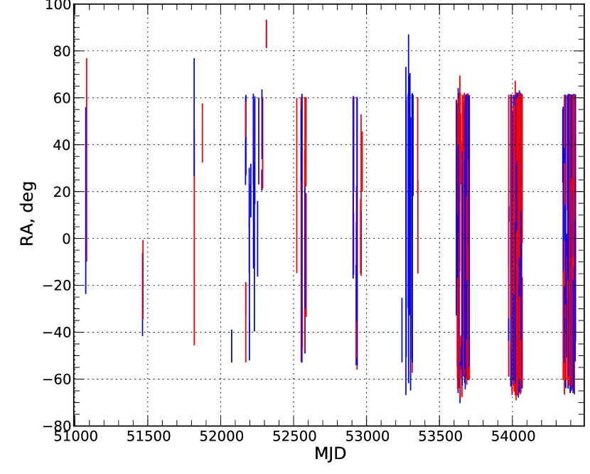
The full database of Stripe 82 contains 303 runs covering nearly 300 deg² of sky along the celestial equator ($-60^{\circ}\leq\rm{RA}\leq 60^{\circ}$ and $-1.25^{\circ}\leq\rm{Decl}\leq 1.25^{\circ}$). The area was scanned repeatedly during 10 years with some regions observed more than 80 times (Abazajian et al., 2009). The SDSS imaging system consists of 30 CCD detectors organized in 6 raws (camcols), where a single CCD in each row is taking data in one of the 5 filters $ugriz$. Since there are gaps between camcols, the width of the major stripe is split into North and South strips covered by independent scans. The SDSS database of Stripe 82 contains 162 North and 141 South runs. The spatial and temporal coverage of all runs is shown in Figure 1, where the blue and red lines correspond to the North and South runs. Each run is divided into $2048\times 1489$ pix sections called fpC frames with a $2049\times 128$ pix margin on both ends (Stoughton et al., 2002). The locations of the beginning and the end of each scan vary from one observation to another. This arrangement is not compatible with subtracting multiple images of the same area, so the runs must be “glued” back together and then subdivided using consistent field boundaries. The rebinning starts from RA_min, the first location covered by at least 20 runs (determined separately for North and South runs). The rearranged frames of $2048\times 1489$ pix are written as FITS files and the process continues untill we reach RA_max, beyond which fewer than 20 runs are available.

Figure 1.— Spatial and temporal coverage of the SDSS Stripe 82 imaging database. North runs are shown in blue and South runs in red. Note a much better time sampling in the later half of the survey.

Some of the data in Stripe 82 were obtained in non-photometric conditions and in relatively poor seeing (DR7). The performance of the difference image analysis method is sensitive to the quality of the images, and therefore our next step is to reject images with poor seeing, high background, and significant background gradients. A small number of images taken toward the ends of the run have strong background gradients due to the Sun or Moon rising or setting. Occasionally, a problem with the bias level subtraction caused a jump in the count level between the left and right parts of the image corresponding to individual amplifiers on the CCD chip. Such images were removed from the analysis. A good quality reference image was prepared for each field using 10 images with the best overall seeing, background, and transparency. This is done with the help of the SExtractor program (Bertin & Arnouts, 1996) by requiring a median $FWHM\leq 1.5"$ for point sources (${\rm CLASS\_STAR}\geq 0.7$) and rejecting background maps with obvious problems. The fields with fewer than 20 remaining images were discarded.

2.2. Difference Image Photometry of SDSS Quasars

Interpolation of images to the same pixel grid was accomplished using approximately 50 stars identified on all images of the field. The time base line of the Stripe 82 data set approaches a decade. We found that a significant fraction of stars shows a detectable proper motion producing time-variable residuals in the shape of a dipole in the difference images (cf. Lacki et al. 2009). In order to limit the impact of such problems on the quality of the final photometry, we selected the reference stars with the proper motion $\mu\leq 100$ mas yr^-1 from the Bramich et al. (2008) catalog in the overlap area (about 50%). The spatial variability of the PSF matching kernel was computed using a third-order polynomial fit to model coefficients and a second-order polynomial for the differential background. Again, slow stars from the catalog of Bramich et al. (2008) were preferentially used to compute the solution. The DIA light curve is computed by adding difference fluxes measured with the DIA package to the flux in the reference image. Object magnitudes were converted to standard SDSS $g$ magnitudes by adding a median offset between stars identified on the reference image and corresponding objects in the SDSS catalog.

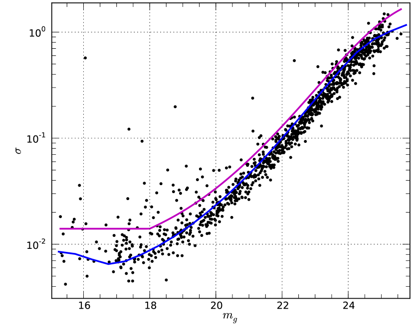
The photometric quality is demonstrated in Figure 2 showing the magnitude scatter versus baseline magnitude for a typical field. Here, the baseline is the median magnitude and the variability of the source is calculated as the 68-th percentile of absolute deviations from the median. Black points correspond to the sources identified in that field and blue line shows median of the variability of the sources from all fields.

In most fields the frame-to-frame accuracy reaches 7 mmag for bright unsaturated sources. For a significant fraction of stars the photometric scatter is worse than that and limited by the residuals due to proper motions. The photometric uncertainty is 1% or better for sources with $m_{g}\leq 18$ and around 10% for sources with $m_{g}\approx 22$. There are 52 quasars with $m_{g}>22$. Those were excluded from the structure function analysis Section 4) due to large uncertainties in their light curves. In the next step, we match spectroscopically confirmed quasars from DR7 Quasar Catalog (Schneider et al., 2010) with our photometric database. There are 9519 DR7 catalog quasars within the area covered by Stripe 82, and we can build DIA light curves for 7614 of them. There are several reasons why we miss a significant number of quasars. After exclusion of poor quality images many fields are left with fewer than 20 epochs and are removed from further analysis. An average 10% of the image area is lost due to masking of very bright stars. Some fields are rejected for lack of stars that can be used to calibrate light curves. Finally, our pipeline occasionally fails on a small fraction of images with problems in fpC frame headers.

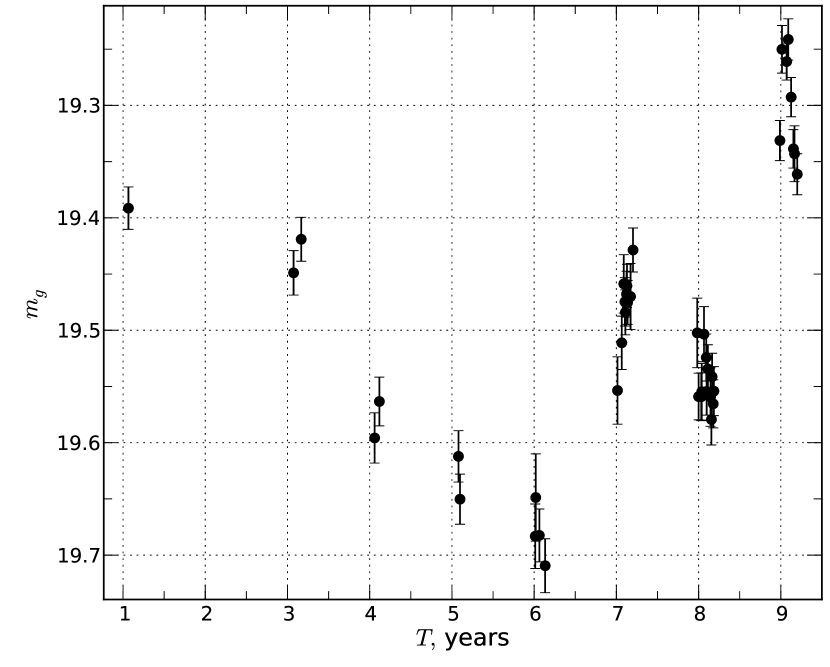
An example quasar light curve resulting from this procedure is shown in the Figure 3. There are 43 observations in the light curve and time counts from the first epoch in Stripe 82 (run 94, fpC frame 12). The number of epochs per quasar in our sample varies between 20 and 56 with the mean of 36.

Figure 2.— Variability diagram in the $g$ band for a typical field in SDSS Stripe 82. The magnitude scatter of all measurements for a given source is plotted against the baseline magnitude (median). The photometry is based on our reanalysis of the SDSS scans using difference image photometry. Black points correspond to the sources identified by SExtaractor. Sources above the magenta line are considered to be variable. Blue line shows median variability of the sources from all fields.

Figure 3.— Example difference imaging light curve for QSO SDSS $223154.15+004747.5$ at $z=0.8409$. Time counts from the first observation in Stripe 82.

3. Structure function

The time sampling of our quasar light curves is relatively sparse (see Figure 3) and insufficient for the use of spectral methods such as the frequency-power spectrum analysis. Following the common practice in AGN variability studies, we focus on the information contained in the structure function. A number of structure function definitions are in use differing in relatively minor details that are not important for this study. We adopt a structure function (hereafter SF) in the form:

$$S(\tau)=\left\{\frac{1}{N(\tau)}\sum_{i<j}(x_{i}-x_{j})^{2}\right\}^{1/2},$$ (1)

where $x_{i}=x(t_{i})$ some random quantity at moment $t_{i}$, the sum is taken over all measurements for which $t_{j}-t_{i}=\tau$ and $N(\tau)$ is the number of such data points. In short, the structure function is a time dependent standard deviation of some random process. SF of white noise is flat and equal to $\sqrt{2\sigma^{2}}$. Therefore, the SF of a random process is also flat on time-scales, where the amplitude of the intrinsic variability is comparable with the measurement errors, as well as on the longest timescales where the r.m.s. stops changing as the length of the time interval keeps increasing. In the context of quasar variability the random quantity is the magnitude (essentially the relative luminosity) $m_{i}$ measured at time $t_{i}$ and $\tau$ is taken in the quasar rest frame. For a given quasar we can write:

$$S^{2}(\tau) = \langle(m_{i}-m_{j})^{2}\rangle_{\tau}\sim\frac{1}{\bar{f}^{2}}\langle(\delta f_{i}-\delta f_{j})^{2}\rangle_{\tau}\equiv$$ (2)

$$\equiv\frac{1}{\bar{L}^{2}}\langle(\delta L_{i}-\delta L_{j})^{2}\rangle_{\tau}=\frac{2\sigma_{\tau}^{2}}{\bar{L}^{2}},$$

where we converted to flux units. The flux consists of a stationary component $\bar{f}$ and a time dependent variable part $\delta f_{i}$, and $\sigma_{\tau}$ is the r.m.s. calculated for points separated by time interval $\tau$. From here it is obvious that for two quasars at the same redshift and with equal $\sigma_{\tau}^{2}$ the brightest one will have smaller variability amplitude, $S(\tau)$, at all time scales.

The number of time intervals that can be constructed from an average of 36 epochs for a single quasar is $36\times(36-1)/2=630$ and results in a very noisy structure function. Therefore, we focus our analysis on the ensemble quasar SF, i.e. we assume that the ensemble variability reflects on average the variability of a single quasar.

4. The Ensemble Structure Function of Quasars

Figure 4.— Top panel: Raw ensemble structure function of 7562 quasars from SDSS Stripe 82 (blue) compared to the structure function for $\sim 1000$ non-variable stars (green). The stars included in this comparison fall below the magenta line in Figure 2) is shown by green points. Bottom panel: Noise-corrected structure function for an ensemble of quasars (blue) and the best fit broken power-law model (red). The oscillations for time-scales above $\sim 100$ days are an artifact of the time sampling. The model offers only an approximate description of the structure function over the full extent of the data.

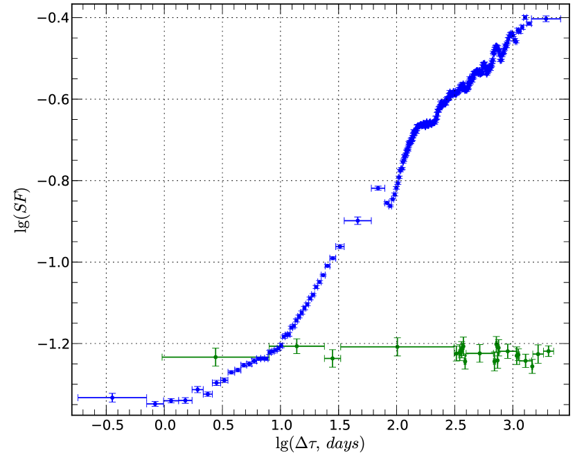
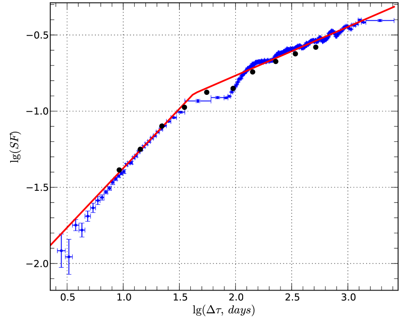
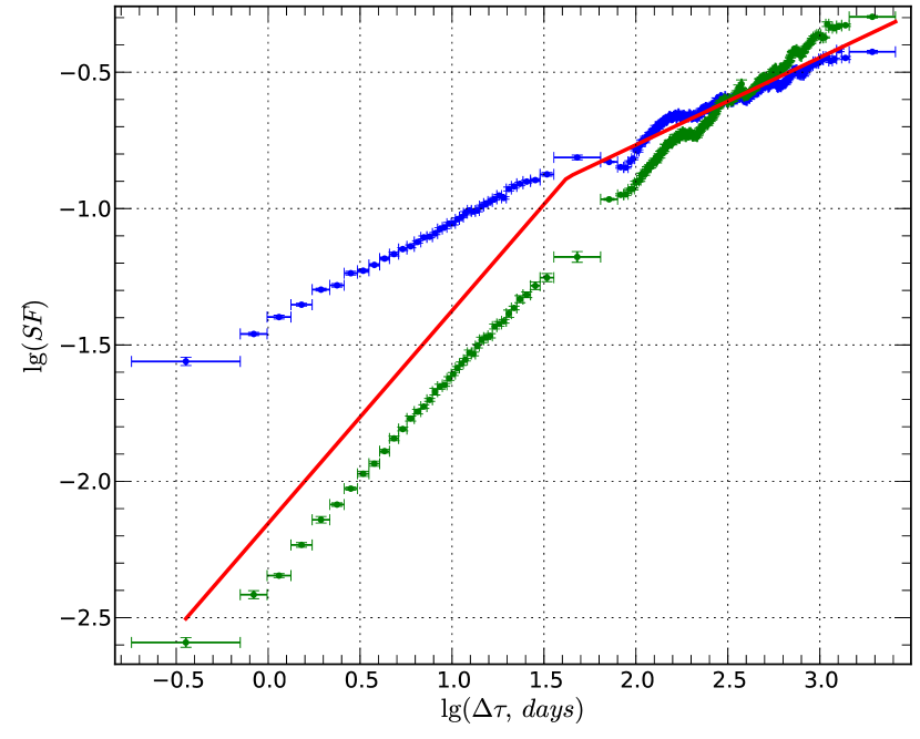
The final sample contains 7562 light curves. All possible pairs of measurements within each light curve are collected for a total of 4,796,468 magnitude differences. After reducing the time lag to the quasar rest frame using spectroscopic redshifts from the SDSS Quasar Catalog (Schneider et al., 2010), the data are binned in time. The bin size was adjusted to reach 20,000 measurements per bin. The resulting ensemble SF consists of 239 bins and is shown in Figure 4 (blue points). Error bars were estimated by dividing each timescale bin into 20 smaller bins, evaluating the mean SF in each, and calculating the r.m.s. scatter of the resulting values (see also de Vries et al. (2005)).

In order to verify that we detect quasar variability and guard against the possibility of contamination by unrelated factors, we repeated this calculation for constant stars. For that purpose we select stars below the magenta line in Figure 2 with $m_{g}\leq 22$. The result is shown in the top panel of Figure 4 (green points). As expected, the SF of non-variable stars is flat over the entire range of time-scales. We conclude that the observed variability of quasars is intrinsic and not caused by unrecognized measurement errors. The stellar structure function exceeds the noise level for the quasar sample because the stars selected for this comparison are fainter on average than the quasars.

The quasar SF in the top panel of Figure 4 displays several slopes and breaks. It starts flat at $\tau\leq 2$ days, then at $2\leq\tau\leq 10$ days gradually transitions to an approximate power-law increase over $10\leq\tau\leq 40$ days, and finally breaks to a shallower slope above $\tau\simeq 100$. The flat portion of the SF is clearly due to noise and the transition to the first power-law section is due to SFs of single quasars with different mean brightness $m_{g}$ reaching the level of noise at different $\tau$ (see Equation 2). The slopes seen at $10\leq\tau\leq 40$ days and $\tau\geq 100$ have a physical origin and are discussed further below. The time interval between 40 and 100 days is poorly sampled and difficult to interpret. This is a result of the SDSS scanning strategy for Stripe 82 that produces relatively few observations separated by 90–270 days in the observer frame (cf. Figure 3) combined with the mean redshift of the sample $\sim 1.5$.

The noise contributes to the SF equally at all timescales and must be subtracted in order to expose the intrinsic quasar variability. The noise-corrected SF is shown in the bottom panel of Figure 4 (blue points). The shape of the quasar SF is dominated by two slopes that we estimate by fitting a broken power law model to the data

$$S(\tau)=\left\{\begin{array}[]{l l}\beta(\tau/\tau_{0})^{\alpha_{1}}&\quad\text{if $\tau\geq\tau_{0}$}\\ \beta(\tau/\tau_{0})^{\alpha_{2}}&\quad\text{if $\tau\leq\tau_{0}$}\\ \end{array}\right..$$ (3)

We find $\alpha_{1}=0.33$, $\alpha_{2}=0.79$, $\tau_{0}=42.3$ days, and $\beta=0.13$ (solid red line). The reduced $\chi^{2}$ of the fit is far from unity, i.e. Equation 3 does not provide a complete description of the data. However, the main goal here is to detect and estimate the two slopes in the overall shape of the SF for an ensemble of quasars, and compare those coefficients with theoretical predictions. We also estimate errors on the derived parameters using ’jackknife’ resampling. Namely, we randomly select 1/3 part of the sample, drop it, and fit ensemble SF built from the rest. We repeat the procedure 100 times and estimate the error on the given parameter as r.m.s. of proper distribution. Such estimation gives very small errors (0.01, 0.02, 3.9 days, and 0.01 for $\alpha_{1}$, $\alpha_{2}$, $\tau_{0}$, and $\beta$ correspondingly) saying that the shape of ensemble SF is quite stable to small variations of the sample.

Figure 5.— Noise-corrected SF^A (blue) and SF^B (green). Black points show the $g$-band structure function from Wilhite et al. (2008) who used the SF^B estimator. Note a close agreement in both the shape and amplitude.

For comparison we plot the $g$-band SF from Wilhite et al. (2008) (black points in the bottom panel of Figure 4). The overall agreement in shape between the SFs is very good and the discrepancy in normalization is explained by the different SF type used in Wilhite et al. (2008). There are two types of SF commonly used in literature. Following Bauer et al. (2009) we refer to them as SF^A and SF^B:

$$S^{A}(\tau) = \sqrt{\langle(\Delta m)^{2}\rangle}$$ (4)

$$S^{B}(\tau) = \sqrt{\frac{\pi}{2}\langle|\Delta m|\rangle^{2}}.$$ (5)

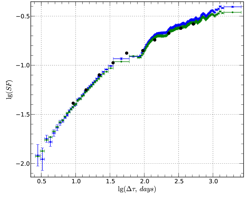
The structure function in the form SF^B was introduced by di Clemente et al. 1996. Our noise-corrected SFs and the $g$-band SF^B from Wilhite et al. (2008) are shown in Figure 5. There is a nearly perfect agreement in both shape and normalization between the B-type SFs derived from the two data sets.

Figure 6.— Light curve simulations. A random simulated light curve (red) is compared with a real light curve of one of the quasars in the sample (blue). The simulated light curves were generated from a power spectrum in the form of a single power-law with the slope $-1.66$ (top) and $-2.58$ (bottom) corresponding to structure functions in Figure 7.

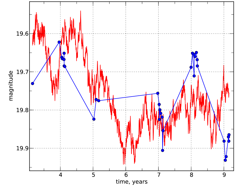
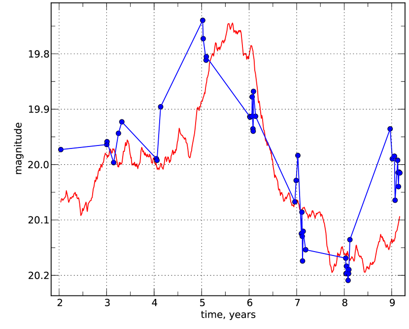
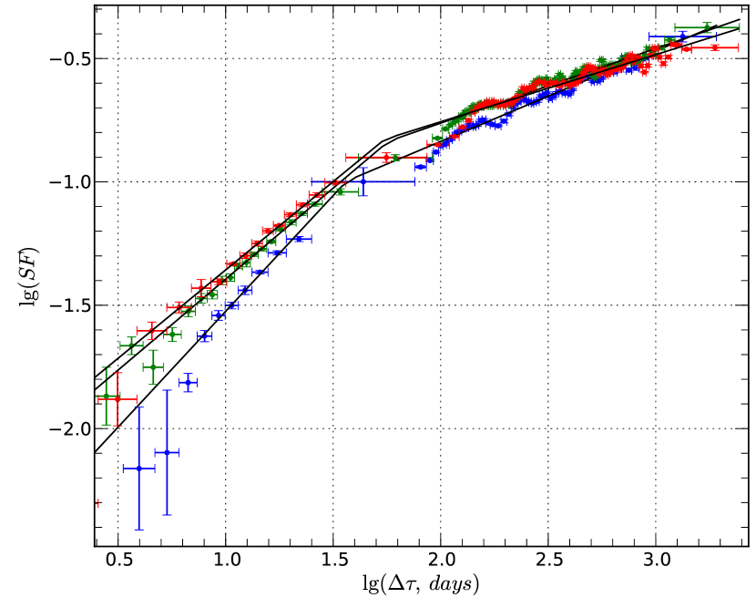
The interpretation of results obtained using SF as a statistical tool is not straightforward. Emmanoulopoulos et al. (2010) show that spurious breaks can appear in the SF due to sparse time sampling and windowing effects. Moreover, the slopes derived from SF modeling are typically much more uncertain than suggested by naive error estimates. Does it mean that the presence of two slopes in Figure 4 is an artifact? To answer this question and validate our results we perform a set of monte-carlo simulations. The goal of this calculation is to verify that for a set of light curves generated from a single power-law spectrum with a given value of $\alpha$ and having the time sampling of real quasars, the algorithm of computing SF does not introduce any significant breaks or biases in the estimated slope.

The simulation is based on the algorithm of Timmer & Koenig (1995) and reproduces both the correct power spectrum as well as the phase mixture. The power spectrum in the form $P(f)\propto f^{-(2\alpha+1)}$ corresponds to SF $S(\tau)\propto\tau^{\alpha}$. We simulate light curves according to a prescription in Emmanoulopoulos et al. (2010). The simulated time series are then normalized to have the same r.m.s. and mean as the real light curves. Examples are shown in the Figure 6.

Figure 7.— Confirming the presence of two slopes in the quasar structure function. The simulated light curves were generated from a power spectrum in the form of a single power-law with the slope $-1.66$ (blue) and $-2.58$ (green) corresponding to the upper and lower portions of the best fit model (red line) from Figure 4.

We simulate two sets of light curves with the power-law spectral density ($-1.66$ and $-2.58$), select points on the simulated light curves corresponding to the time sampling of a real light curve, and apply proper rest frame correction. In Figure 7 the simulated SFs are compared to the best fit model for real quasars. The slopes of the simulated SFs do not exactly match the slope of the model from which they were generated, i.e. the time sampling slightly biases the measured shape of the SF. However, none of the simulated SFs is even close to a broken power law with $\alpha_{1}=0.33$ and $\alpha_{2}=0.79$. Therefore, the large observed difference in the SF slope between the short and long timescales is not due to the time sampling, but rather of a physical origin. Possible interpretations are discussed in the next section.

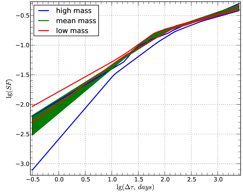
The ensemble SF considered here is built from quasars with different intrinsic characteristics such as black hole mass or luminosity. Therefore, it is interesting to check whether two slopes in SF are characteristic for the hole range of, say, black hole masses or have dependence on mass. Using black hole mass estimations from Shen et al. (2008), we select three subsamples of quasars with black hole masses in ranges $\leq 5\times 10^{8}\,M_{\odot}$ (1953 sources, low mass range), $5\times 10^{8}\div 1.5\times 10^{9}M_{\odot}$ (2108 sources, mean mass range), $\geq 1.5\times 10^{9}M_{\odot}$ (1276 sources, high mass range) and build SF for each range of masses. All three SFs show existence of two slopes (see Figure 8, top panel). We fit SFs by broken power low model (Equation 3). The best fit parameters and formal estimation of errors by ’jackknife’ resampling are given in the Table 1. In order to have better understanding of the uncertainties in the parameters we also plot regions showing minimal and maximal values of the fits for all three SFs (see Figure 8, bottom panel). As it is seen from the Figure 8, the SFs slopes tend to increase with the growth of the mean subsample mass but still have common values. More subtle study is needed in order to show that the trend in slopes as a function of black hole mass is real. Here we only conclude that the presence of two slopes in the ensemble SF is independent on the considered black hole mass range.

Figure 8.— Top panel: Ensemble SF for quasars with black hole masses lying in low mass range (red points), mean mass range (green points ), and high mass range (blue points) (see text for definition of ranges). Thin black lines show best fits for each SF. Bottom panel: Regions showing the scatter of the best fits obtained during ’jackknife’ resampling. Red lines show the scatter of the low mass range SFs best fits, green region and blue lines show the same for mean mass and high mass ranges correspondingly.

Table 1Best fit parameters

Subsample	$\alpha_{1}$	$\alpha_{2}$	$\tau_{0}$, days	$\beta$
low mass	$0.27\pm 0.02$	$0.72\pm 0.04$	$55.0\pm 16.7$	$0.15\pm 0.02$
mean mass	$0.30\pm 0.01$	$0.74\pm 0.03$	$57.3\pm 6.6$	$0.15\pm 0.02$
high mass	$0.37\pm 0.02$	$0.94\pm 0.09$	$36.6\pm 15.6$	$0.10\pm 0.02$

5. Discussion

We consider three processes frequently invoked to explain the variability of quasars: instabilities in the accretion flow around a supermassive black hole, supernova explosions related to the starburst phenomenon, and gravitational microlensing by compact bodies in the host galaxy (Kawaguchi et al., 1998; Hawkins, 2002). SFs of light curves predicted by each model are characterized by different slopes. The expected SF slopes are $0.25\pm 0.03$, $0.44\pm 0.03$, $0.83\pm 0.08$ respectively for variability generated by miscrolensing, disk instability, and starburst mechanisms (Hawkins, 2002). The SF slopes found in Section 4 are 0.79 and 0.33 correspondingly for time lags below and above $42$ days. Taken at face value, the first slope is consistent with the starburst model, and the second slope falls half way between the predictions of the disk instability model and the microlensing model. Note that SF slopes in the range 0.30–0.35 have been obtained in other works, but the authors still attributed the variability to disk instabilities. Bauer et al. (2009) and Meusinger et al. (2011) present an overview of recent results.

Figure 9.— Testing the asymmetry in the quasar structure function between the leading and trailing branch of a typical flare. Flux increases contribute to $S_{+}$ (blue) and flux drops contribute to $S_{-}$ (green).

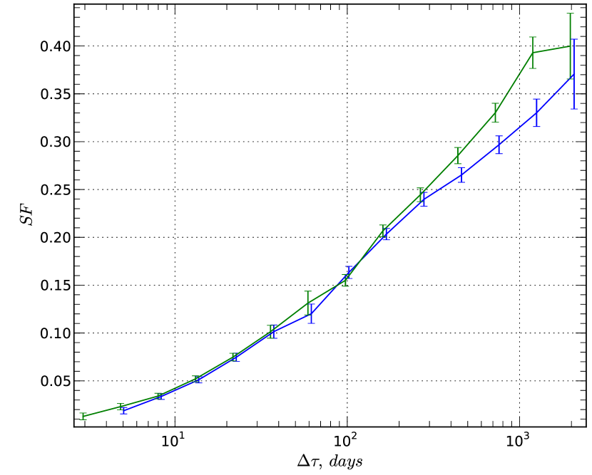
Asymmetries in the SF provide an additional test of model predictions. The SF that only includes those pairs of measurements for which the flux increases with time, $S_{+}$, may be different from $S_{-}$, the SF characterizing a decrease in flux. Kawaguchi et al. (1998) show that in starburst models $S_{+}>S_{-}$. Disk instabilities produce $S_{-}>S_{+}$ and microlensing is symmetric, i.e. $S_{-}=S_{+}$ when averaged over sufficiently long time intervals (Hawkins, 2002). The difference between $S_{-}$ and $S_{+}$ depends on the parameters of the model and therefore $S_{-}\simeq S_{+}$ is still possible in both the starburst and the disk instability model (Kawaguchi et al., 1998).

Noise-corrected $S_{+}$ and $S_{-}$ functions are shown in Figure 9 with blue and green lines respectively. For long time lags in the range 300–1600 days, where the SF slope is $\sim 0.33$, we have $S_{-}>S_{+}$, as predicted by the disk instability model. The significance of the difference is not very high, but allows us to exclude the microlensing model. The difference disappears for time-scales below 100 days, where the slope is consistent with the starburst model. This may suggest that a typical supernova rate in a starbursts in the host galaxies of quasars is as high as $\sim 100$ yr^-1 and effectively washes out any detectable asymmetry (see Fig. 6 in Kawaguchi et al. (1998)). However, the rate should be treated with caution since it is not derived from direct measurements. Moreover, the predictions for $S_{+}$ and $S_{-}$ were derived from simulations of a single variability mechanism. The addition of another variability process can wash out the difference between $S_{+}$ and $S_{-}$. This is an interesting topic for future research. The difference in $S_{+}$ and $S_{-}$ was also investigated by de Vries et al. (2005) and Bauer et al. (2009). The former study found tentative evidence that $S_{+}>S_{-}$ (light curves have fast rise and slow decay as in starburst model) for 400 days $\leq\tau\leq$ 1500 days, while in the latter work $S_{+}\approx S_{-}$ over the full range of measurements ($\tau\leq 1000$ days). The explanation of the difference in results is difficult because each paper is based on entirely different data and requires further research. The de Vries et al. (2005) analysis relies on cross survey flux comparisons.

The introduction of the supernova variability mechanism may be redundant as the shape of the SF can be explained by detailed variability mechanisms acting in accretion disks. For instance, the PSD of X-ray light curves of some active galactic nuclei have two (e.g.  Summons et al. (2007)) or more distinct slopes (McHardy et al., 2007). Considering that the optical emission tends to follow the X-ray flux with some time delay one may expect that PSDs of optical light curves will display two slopes. Moreover, the SF shape found here is in qualitative agreement with the model proposed in Arévalo et al. (2009), where large amplitude optical variations on the time scales of hundreds of days are attributed to the fluctuations in accretion rate and short-term (order of days), small amplitude variations arise due to reprocessing of X-rays.

6. Summary

We applied the image differencing technique to the entire $g$-band imaging data set of SDSS Stripe 82 and constructed high quality light curves for 7562 spectroscopically identified quasars with no less then 20 epochs. The variability analysis was performed using the ensemble structure function. While the shape and normalization of the quasar structure function derived here are in perfect agreement with the results of Wilhite et al. (2008) based on an earlier SDSS data release, our structure function is estimated from a much larger data set and covers a substantially wider range of time lags from 8 hours to 6.9 years in the quasar rest frame.

We find that the ensemble SF reveals two distinct power-law slopes with the break around $42$ days and confirm the presence of these features with monte-carlo simulations. The presence of two slopes in the ensemble SF is independent on the black hole mass range of quasars used to build it. The slopes estimated from a broken pawer-law fit to the data are $\alpha_{1}\simeq 0.79$ for $\tau\leq 100$ days and $\alpha_{2}\simeq 0.33$ for $\tau\geq 300$ days. Using predictions from the theoretical models, the variability of quasars on times scales $\tau\leq 100$ days can be explained by a starburst model. The slope of the structure function on time-scales longer than about 3 months is rather close to models where variability is explained by gravitational microlensing. However, on time-scales $\tau\geq 300$ days we detect a significant asymmetry in the SF characteristic for disk instabilities that rules out a substantial contribution of microlensing. It is also possible to explain the shape of SF without invoking the starburst model, but using the model, where short term optical variations are caused by X-rays reprocessing and long therm variations originate from optical emitting regions of accretion disk (Arévalo et al., 2009).

The existing SDSS Stripe 82 data offer a great opportunity to better understand the origin of variability in quasars. The main limiting factor at present is the lack of detailed theoretical predictions that go beyond the basic characteristics such as the SF slope and include the detailed shape and normalization of the SF, as well as asymmetries and color information.

References

- Abazajian et al. (2009) Abazajian, K. N., et al. 2009, ApJS, 182, 543
- Alard (2000) Alard, C. 2000, A&AS, 144, 363
- Alard & Lupton (1998) Alard, C., & Lupton, R. H. 1998, ApJ, 503, 325
- Aretxaga et al. (1997) Aretxaga, I., Cid Fernandes, R., & Terlevich, R. J. 1997, MNRAS, 286, 271
- Arévalo et al. (2009) Arévalo, P., Uttley, P., Lira, P., Breedt, E., McHardy, I. M., & Churazov, E. 2009, MNRAS, 397, 2004
- Bauer et al. (2009) Bauer, A., Baltay, C., Coppi, P., Ellman, N., Jerke, J., Rabinowitz, D., & Scalzo, R. 2009, ApJ, 696, 1241
- Bertin & Arnouts (1996) Bertin, E., & Arnouts, S. 1996, A&AS, 117, 393
- Bramich et al. (2008) Bramich, D. M., et al. 2008, MNRAS, 386, 887
- Cid Fernandes et al. (1996) Cid Fernandes, R., Jr., Aretxaga, I., & Terlevich, R. 1996, MNRAS, 282, 1191
- de Vries et al. (2005) de Vries, W. H., Becker, R. H., White, R. L., & Loomis, C. 2005, AJ, 129, 615
- di Clemente et al. (1996) di Clemente, A., Giallongo, E., Natali, G., Trevese, D., & Vagnetti, F. 1996, ApJ, 463, 466
- Emmanoulopoulos et al. (2010) Emmanoulopoulos, D., McHardy, I. M., & Uttley, P. 2010, MNRAS, 404, 931
- Hawkins (2002) Hawkins, M. R. S. 2002, MNRAS, 329, 76
- Hawkins (2007) Hawkins, M. R. S. 2007, A&A, 462, 581
- Kawaguchi et al. (1998) Kawaguchi, T., Mineshige, S., Umemura, M., & Turner, E. L. 1998, ApJ, 504, 671
- Kelly et al. (2009) Kelly, B. C., Bechtold, J., & Siemiginowska, A. 2009, ApJ, 698, 895
- Kochanek et al. (2006) Kochanek, C. S., Mochejska, B., Morgan, N. D., & Stanek, K. Z. 2006, ApJ, 637, L73
- Kozlowski et al. (2010) Kozlowski, S. et al. 2010, ApJ708, 927
- Lacki et al. (2009) Lacki, B. C., Kochanek, C. S., Stanek, K. Z., Inada, N., & Oguri, M. 2009, ApJ, 698, 428
- McHardy et al. (2007) McHardy, I. M., Arévalo, P., Uttley, P., Papadakis, I. E., Summons, D. P., Brinkmann, W., & Page, M. J. 2007, MNRAS, 382, 985
- McLeod et al. (2010) MacLeod, C. L. et al. 2010, ApJ721, 1014
- Meusinger et al. (2011) Meusinger, H., Hinze, A., & de Hoon, A. 2011, A&A, 525, A37
- Pereyra et al. (2006) Pereyra, N. A., Vanden Berk, D. E., Turnshek, D. A., Hillier, D. J., Wilhite, B. C., Kron, R. G., Schneider, D. P., & Brinkmann, J. 2006, ApJ, 642, 87
- Palanque-Delabrouille et al. (2011) Palanque-Delabrouille, N., et al. 2011, A&A, 530, A122
- Schmidt et al. (2010) Schmidt, K. B., Marshall, P. J., Rix, H.-W., Jester, S., Hennawi, J. F., & Dobler, G. 2010, ApJ, 714, 1194
- Schneider et al. (2010) Schneider, D. P., et al. 2010, AJ, 139, 2360
- Shen et al. (2008) Shen, Y., Greene, J. E., Strauss, M. A., Richards, G. T., & Schneider, D. P. 2008, ApJ, 680, 169
- Stoughton et al. (2002) Stoughton, C., et al. 2002, AJ, 123, 485
- Summons et al. (2007) Summons, D. P., Arévalo, P., McHardy, I. M., Uttley, P., & Bhaskar, A. 2007, MNRAS, 378, 649
- Terlevich et al. (1992) Terlevich, R., Tenorio-Tagle, G., Franco, J., & Melnick, J. 1992, MNRAS, 255, 713
- Timmer & Koenig (1995) Timmer, J., & Koenig, M. 1995, A&A, 300, 707
- Vanden Berk et al. (2004) Vanden Berk, D. E., et al. 2004, ApJ, 601, 692
- Wilhite et al. (2008) Wilhite, B. C., Brunner, R. J., Grier, C. J., Schneider, D. P., & vanden Berk, D. E. 2008, MNRAS, 383, 1232
- Woźniak (2000) Woźniak, P. R. 2000, Acta Astronomica, 50, 421