Recursions in Calogero-Sutherland Model Based on Virasoro Singular Vectors

1 Introduction and Conclusion

The Calogero-Sutherland (CS) Model, which is an integrable 1d many-body system, plays important roles in many different research areas in physics and mathematics. Among them are the 2D conformal field theories(CFTs)[1, 16], the generalized matrix models[2, 4], the fractional quantum hall effects(FQHE) [6, 7, 11, 12], and there is an even more surprising correspondence related to the $N=2^{\ast}$ 4D supersymmetric gauge systems[23, 24, 25, 26, 27, 28, 29]. The spectrum of the CS model can be generated from the Jack polynomials[5, 17, 18, 19, 32]. From the CFT point of view, Jack symmetric functions are naturally the building blocks for the conformal towers, the characters of which encode the (extended) conformal symmetries. For instance, the Jack functions related to a given Young tableaux are believed to be in one to one correspondence with the singular vectors of the $W$-algebra[1], which reflects the hidden $W_{1+\infty}$ symmetry of the CS model. Singular vectors in 2d CFT are the keys to the calculation of the correlation functions in CFT and may also reveal important physical properties of the CS model. Unfortunately, on the CFT side, it is not clear how to relate the construction of the secondary states in the conformal tower to that of the Jack functions, except for some simple cases, i.e. the Virasoro singular vectors [10]. On the 2d CFT side, the calculation of conformal blocks is based on the conformal Ward-identities,

$$[L_{n},V_{h}(z)]=(z^{n+1}\partial_{z}+(n+1)hz^{n})V_{h}(z).$$

And the calculation is carried out perturbatively level by level [8, 9]. In some special cases, the decoupling of the Virasoro null vectors can be implemented as differential equations for the conformal blocks. For the general case, recursion relations have been proposed by Zamolodchikov on the meromorphic structures of the conformal blocks either in complex $c$-plane or $h$-plane. However, it remains unclear (to us) how to construct the basis vectors in the given conformal tower by making use of the Zamolodchikov’s recursion formulae explicitly. In contrast, there are various ways in the explicit constructions of the Jack polynomials, each follows different strategies. For example, there are two integral representations. The one given in [3] is based on the $W_{1+\infty}$ symmetry hidden in the CS model, the other, by the authors of [13], starts from the so called shift Jack polynomials. There is also an operator formalism [14, 15] based on the Dunkel (exchange) operators. However, here we follow a different strategy in constructing the Jack polynomials which are intrinsically related to the singular vectors in the Virasoro algebra, and present a new recursion relation derived from the construction. We also do not need to invoke the hidden $W$-algebra. In fact there is a hidden Virasoro structure in the Hilbert space of the CS model which can be used recursively in our construction. To be more specific, the ket states in the Fock space realization of the CS model is mapped a la Feigin-Fuks-Dotsenko-Fateev Coulomb gas formalism [20][21] to the singular vectors of the Virasoro algebra and its skew hierarchical descendants. The construction of the singular vectors defines a new recursion relation for the Jack functions and finally leads to a new integral representation which differs from the one appeared in [3, 13]. Hence our approach may supply new insights in dealing with CS model or more general integrable systems.

The structure of this article is organized as following. In section 2, we review some useful properties of the Jack polynomials and the CS model. In section 3, we review the construction of the Virasoro singular vectors which are related to the Jack polynomials with rectangular Young tableaux. It should be stressed again that the Virasoro symmetry is hidden in the ket (or bra) Hilbert space only, and is not the true symmetry in the CS model. The reason is that the prescribed Hermiticity in the CS model is not respected by the conjugation of the hidden Virasoro algebra. I.E., the Virasoro structure in the bra and ket Hilbert spaces, respectively, are not related by the Hermitian conjugation in the CS model. Our main results are given in sections 4 and 5. In section 4, we propose a skew (recursion) formula for generating new Jack functions stating from the simple ones which inevitably involve the Virasoro singular vectors, or equivalently, the Jack functions of the rectangular graph. Our proof of the skew (recursion) formula can be considered as an operator formalism generalization of its counterpart for the Jack symmetric polynomials found by Kadell in [18]. The basic skew relation is further developed recursively in section 5. This can be made explicit first in the operator formalism, based on which we develop a new integral representation for the Jack symmetric functions associated with any generic Young tableaux. One immediately sees the advantages of our operator formalism of the skew (recursion) formula over the one proposed by Kadell. Since our formalism does not depend on explicitly the number of argument variables $\{z_{i}\}$ for $i=1,\cdots,N$, so the recursion is done without worrying the change of the total number of arguments. Finally, the integral representation of the Jack symmetric polynomials which depend explicitly on finite number of variables $\{z_{i}\}$, for $i=1,\cdots,N$, are presented as a by-product.

2 Jack Polynomials and Calogero-Sutherland Model

Now we review the Jack polynomials and the Calogero-Sutherland model. The Jack polynomials can be viewed as a special one parameter generalization of the Schur polynomials[32] and the Jack symmetric function is the large N limit of the Jack polynomials. For physicists, the most familiar integrable system which involves Jack symmetric functions as its spectrum functions is the Calogero-Sutherland model. This model is an integrable system and shows a great deal of interesting aspects, such as duality, conformal invariance, and even the combinatorial property of the spectrum etc. An elementary introduction can be found, for instance, in [11] and further studies in [19] and [32]. Here we only review some basics of the Jack polynomials.

2.1 Partitions and Jack Polynomials

Given a partition: $\lambda=(\lambda_{1},\lambda_{2},\dots,\lambda_{n})$, $\lambda_{1}\geq\lambda\geq\cdots\geq\lambda_{n}$ ,$n\equiv l(\lambda)$, one defines the related Jack polynomial as the basis function for the symmetric homogeneous polynomials in $N$ variables $\{z_{i}\},i=1,2,...,N$, of degree $|\lambda|=\sum\lambda_{i}$

$$J_{\lambda}(\{z_{i}\})=\sum_{\lambda^{\prime}\leq\lambda,\,l(\lambda^{\prime})\leq N}C_{\lambda}^{\lambda^{\prime}}z^{\lambda^{\prime}}\,,$$ (1)

which should satisfy the second order differential equation:

$$H_{J}J_{\lambda} = E_{\lambda}J_{\lambda},\,\,\,\,\,H_{J}=H_{J}^{0}+\beta H_{J}^{I}$$ (2)

$$H_{J}^{0} = \sum_{i}^{N}\left(z_{i}\partial_{z_{i}}\right)^{2},\,\,\,\,H_{J}^{I}=\sum_{i<j}\dfrac{z_{i}+z_{j}}{z_{i}-z_{j}}(z_{i}\partial_{z_{i}}-z_{j}\partial_{z_{j}})\,,$$ (3)

here

$$z^{\lambda}:=\sum_{P}z_{P(1)}^{\lambda_{1}}\cdots z_{P(N)}^{\lambda_{N}}\,,$$ (4)

$$\lambda^{\prime}\leq\lambda\Rightarrow\sum_{i=1}^{j}\lambda^{\prime}_{i}\leq\sum_{i=1}^{j}\lambda_{i},\,for\,j=1,2,\cdots l(\lambda^{\prime})$$

$P$ means the permutations of $N$ objects. We have also defined $\lambda_{i}=0$ for $i>l(\lambda)$ and $\lambda_{1}+\lambda_{2}+\cdots+\lambda_{l(\lambda)}=|\lambda|$, $|\lambda|$ is the level of the partition. $\lambda$ can be represented graphically as a Young tableau $\lambda=\{(i,j)|1\leq i\leq l(\lambda)\},1\leq j\leq\lambda_{i}$. And the corresponding transposed Young tableau is represented as

$$\lambda^{t}=(\lambda^{t}_{1},\lambda^{t}_{2},\dots,\lambda^{t}_{\lambda_{1}})\Rightarrow\lambda=(\lambda_{1},\lambda_{2},\dots,\lambda_{\lambda^{t}_{1}}).$$

It is clear that $l(\lambda)\equiv\lambda^{t}_{1}$. We shall see later that the defining differential equation can be derived from the CS Hamiltonian.

The Jack polynomials can be generated by the power sum symmetric polynomials as well: $p_{l}=\sum_{i=1}^{N}z_{i}^{l}$

$$J_{\lambda}(p)=\sum_{|\lambda^{\prime}|=|\lambda|}d_{\lambda}^{\lambda^{\prime}}p_{\lambda^{\prime}},\ \ \ p_{\lambda^{\prime}}=p_{\lambda^{\prime}_{1}}p_{\lambda^{\prime}_{2}}\cdots p_{\lambda^{\prime}_{m}},\ \ \ d_{\lambda}^{1^{|\lambda|}}=1$$

when $N$ large, $J_{\lambda}$ spans the Hilbert space of free oscillators, and each power sum symmetric polynomial behaves as a single oscillator. By using the conjugacy class representation of the Young tableau $\lambda=\{i^{m_{i}}\},~{}~{}i=1,2,\dots$, where $m_{i}$ means the multiplicity of the rows of $i$ squares in Young tableau $\lambda$, the normalization of the power sum symmetric polynomial is derived from that of the oscillators,

$$\langle p_{\lambda},p_{\lambda^{\prime}}\rangle = \langle\frac{a_{\lambda}a_{-\lambda^{\prime}}}{\beta^{\frac{1}{2}l(\lambda)}\beta^{\frac{1}{2}l(\lambda^{\prime})}}\rangle$$

$$= \delta_{\lambda\lambda^{\prime}}i^{m_{i}}m_{i}!\beta^{-l(\lambda)}$$

$$\langle a_{n}a_{-m}\rangle = \delta_{n,m}n,\,\,\,\beta=k^{2}\,,$$

In fact, the above normalization is consistent with that of Jack symmetric functions[11, 19]. The normalization of the Jack polynomials is derived from that of the wave function in the CS model:

$$\left(\prod_{i}^{N}\int_{0}^{\pi}dx_{i}\right)J_{\lambda^{\prime}}(p^{\ast})J_{\lambda}(p)\prod_{i<j}|z_{i}-z_{j}|^{2\beta}=\Gamma_{N}^{2}\delta_{\lambda,\lambda^{\prime}}j_{\lambda}\dfrac{\bar{A}_{\lambda,N}}{\bar{B}_{\lambda,N}}\,,$$ (6)

here

$$j_{\lambda} = A_{\lambda}^{1/{\beta}}B_{\lambda}^{1/\beta},\,\,\,z_{i}=e^{2ix_{i}}$$ (7)

$$A_{\lambda}^{1/\beta} = \prod_{s\in\lambda}\left(a_{\lambda}(s)\beta^{-1}+l_{\lambda}(s)+1\right),\,\,\,B_{\lambda}^{1/\beta}=\prod_{s\in\lambda}\left((a_{\lambda}(s)+1)\beta^{-1}+l_{\lambda}(s)\right)\,$$

$a_{\lambda}(s)$ and $l_{\lambda}(s)$ are called arm-length and leg-length of the box $s$ in the Young tableau $\lambda$:

$$a_{\lambda}(s)=\lambda_{i}-j,\,\,\,\,\,l_{\lambda}(s)=\lambda^{t}_{j}-i,$$

$\lambda^{t}_{j}$ is the $j$-th part of the partition related to the transposed Young tableau $\lambda$.

$$\bar{A}_{\lambda,N}=\prod_{s\in\lambda}\left(N+a^{\prime}_{\lambda}(s)/\beta-l^{\prime}_{\lambda}(s)\right),\,\,\,\,\bar{B}_{\lambda,N}=\prod_{s\in\lambda}\left(N+(a^{\prime}_{\lambda}(s)+1)/\beta-(l^{\prime}_{\lambda}(s)+1)\right),$$

$a^{\prime}_{\lambda}(i,j)=j-1$, $l^{\prime}_{\lambda}(i,j)=i-1$ denote the co-arm-length and co-leg-length for the box $s=(i,j)$ in Young tableau $\lambda$. $\Gamma_{N}^{2}\equiv\pi^{N}\dfrac{\Gamma(1+N\beta)}{\Gamma^{N}(1+\beta)}$ is the normalization of the ground state. When $N\to\infty$, and after dividing out the ground state normalization $\Gamma_{N}^{2}$, we obtain the normalization for the Jack functions:

$$\langle J_{\lambda},J_{\lambda^{\prime}}\rangle = \int J_{\lambda^{\prime}}(p^{\ast})J_{\lambda}(p)\dfrac{\prod_{i<j}|z_{i}-z_{j}|^{2\beta}}{\Gamma_{N}^{2}}\prod_{i=1}^{N}dx_{i}\mid_{N\to\infty}=\delta_{\lambda,\lambda^{\prime}}j_{\lambda}$$ (8)

We shall see in the next section that eq.(6) implies the following integral formula

$$J_{\lambda}(\dfrac{a_{-}}{k})=\int e^{k\sum_{n>0}\frac{a_{-n}}{n}p_{n}}J_{\lambda}(p^{\ast})\dfrac{\prod_{i<j}|z_{i}-z_{j}|^{2\beta}}{\Gamma_{N}^{2}}\prod_{i=1}^{N}dx_{i}\,.$$ (9)

Now we shall clarify some notations used in this work. $J_{\lambda}(p)$ means Jack polynomials in the power sum polynomial basis, $J_{\lambda}(\frac{a}{k})$ the annihilation operator valued Jack symmetric function, i.e. with the substitution $p_{n}\rightarrow\dfrac{a_{n}}{k}$, and $J_{-\lambda}\equiv J_{\lambda}(\frac{a_{-}}{k})$ the creation operator valued Jack symmetric function, i.e. with the substitution $p^{\ast}_{n}\rightarrow\dfrac{a_{-n}}{k}$.

2.2 Calogero-Sutherland Model

The CS model is introduced for studying Coulomb interacting electrons distributed on a circle. The Hamiltonian for this system can be written as:

$$H_{CS} = -\sum_{i=1}^{N}\frac{1}{2}\partial_{i}^{2}+\sum_{i<j}\frac{\beta(\beta-1)}{\sin^{2}(x_{ij})}$$ (10)

here $\partial_{i}=\partial_{x_{i}},\,\hbar^{2}/8m=1$, $\beta=k^{2}$, $k$ is the charge of the N identical electrons. This is an exact solvable system. However, let’s consider another auxiliary Hamiltonian which is positive definite and differs from the original one only by a shift of the constant ground state energy

$$H = -\frac{1}{2}\sum_{i=1}^{N}(\partial_{i}+\partial_{i}\ln\prod_{l<j}\sin^{\beta}x_{lj})(\partial_{i}-\partial_{i}\ln\prod_{l<j}\sin^{\beta}x_{lj})$$

$$= -\frac{1}{2}\sum_{i=1}^{N}\partial_{i}^{2}+\beta(\beta-1)\sum_{i<j}\frac{1}{\sin^{2}x_{ij}}-\frac{1}{6}\beta^{2}N(N+1)(N-1)$$

$$= H_{CS}-E_{0}\,,$$

$$E_{0} = \frac{1}{6}\beta^{2}N(N+1)(N-1)\,.$$

In going from the first line to the second line of eq. (2.2), we have used the identity

$$\sum_{i,j\neq k}\cot x_{ij}\cot x_{ik}+\sum_{j,i\neq k}\cot x_{ji}\cot x_{jk}+\sum_{k,i\neq j}\cot x_{ki}\cot x_{kj}$$

$$= \sum_{i,j\neq k}\frac{-\cos x_{ij}-\cos x_{ik}\cos x_{jk}}{\sin x_{ik}\sin x_{jk}}$$

$$= \sum_{i,j\neq k}(-1)=-N(N-1)(N-2)\,.$$

where $x_{ij}\equiv x_{i}-x_{j}$. It is also convenient to define $z_{i}=e^{2ix_{i}}$ for later use. The ground state should be a solution to the eigen-equation:

$$H_{CS}\psi_{0}=E_{0}\psi_{0},$$

and can be easily read out:

$$\psi_{0}=\prod_{i<j}(2\sin^{\beta}x_{ij})\,,$$

where the factor of 2 is included for normalization reason. If one defines the excited state as

$$\psi_{\lambda}=J_{\lambda}\psi_{0}\,,$$

then it can be shown that this state actually satisfies the energy eigen-equation:

$$H\psi_{\lambda} = H\psi_{0}J_{\lambda}(p)=\psi_{0}(\psi_{0}^{-1}H\psi_{0})J_{\lambda}(p)$$

$$= 2\psi_{0}H_{J}J_{\lambda}(p)=2\psi_{0}E_{\lambda}J_{\lambda}(p)\,,$$

$$H_{J} = \frac{1}{2}\psi_{0}^{-1}H\psi_{0}=-\frac{1}{4}\sum_{i=1}^{N}(\partial_{i}+2\beta\sum_{j\neq i}\cot x_{ij})\partial_{i}\,,$$ (14)

thus the eigen-equation can be rewritten as

$$H_{J}J_{\lambda} = \left[-\dfrac{1}{4}\sum_{i=1}^{N}\partial_{i}^{2}-\dfrac{1}{2}\beta\sum_{i<j}\cot x_{ij}(\partial_{i}-\partial_{j})\right]J_{\lambda}=E_{\lambda}J_{\lambda}\,.$$ (15)

We see that this coincides with the defining differential equation eq.(2) for the Jack polynomials. The eigenstates of $H_{J}$ in the form of eq.(14) and(15), means that $H_{J}$ is triangular with respect to the symmetric monomials.

$$J_{\lambda}\sim\left(\prod_{i=1}^{l(\lambda)}z_{i}^{\lambda_{i}}+symmetrization\right)+daughter\,\,\,terms\,.$$

Here the daughter terms are the symmetrized monomials associated with Young tableau $\lambda^{\prime}<\lambda$. That is to say, given a Young tableau $\lambda$, one can squeeze the partition $\{\lambda\}$ to other partitions by moving squares in $\lambda$ downwards to get new Young tableaux. These terms actually reflect the triangular property of the interaction $H_{J}^{I}$ as in eq.(2). fig.1 gives an example of squeezing.

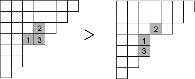
Figure 1: An example for squeezing Young tableau, where the square 3 has been squeezed downward to form a different Young tableau.

It is easy to read out the eigenvalue of $H_{J}$ which can be read off from the diagonal value of the leading term of the eigenstate

$$E_{\lambda} = -\frac{1}{4}\sum_{i}^{N}(-4\lambda_{i}^{2})-constant\,\,term\,\,part\,\,\left(\frac{1}{2}\sum_{i<j}i\beta\frac{(z_{i}+z_{j})}{(z_{i}-z_{j})}\frac{(z_{i}^{\lambda_{i}}z_{j}^{\lambda_{j}}-z_{j}^{\lambda_{i}}z_{i}^{\lambda_{j}})}{(z_{i}^{\lambda_{i}}z_{j}^{\lambda_{j}}+z_{j}^{\lambda_{i}}z_{i}^{\lambda_{j}})}(2i\lambda_{i}-2i\lambda_{j})\right)$$ (16)

$$= \sum_{i}^{N}\lambda_{i}^{2}+\beta\sum_{i<j}(\lambda_{i}-\lambda_{j})$$

$$= \sum_{i}^{N}\lambda_{i}^{2}+\beta\sum_{i}^{N}(N-2i+1)\lambda_{i}\,.$$

Here in the last step of eq.(16), we have used the fact that

$$\sum_{i<j}^{N}(\lambda_{i}-\lambda_{j}) = (N-1)\lambda_{1}+(N-2-1)\lambda_{2}+\cdots+(N-2i+1)\lambda_{i}\cdots$$

$$= \sum_{i}^{N}(N-2i+1)\lambda_{i}\,.$$

Here, since we are concerning ourselves to all the Young tableaux $\lambda^{\prime}\leq\lambda$ with the restriction $l(\lambda^{\prime})\leq N$, so we redefine $\lambda$ as well as $\lambda^{\prime}$ to include the trailing null parts such that $l(\lambda^{\prime})=l(\lambda)=N$. Actually, eq.(16) can be written as the following more compact formula:

$$E_{\lambda} = k\left(k^{-1}||\lambda||^{2}-k||\lambda^{t}||^{2}+kN|\lambda|\right)$$ (17)

$$||\lambda||^{2} \equiv \sum_{i}^{N}\lambda_{i}^{2},\,\,\,\,||\lambda^{t}||^{2}\equiv\sum_{i}^{N}(\lambda_{i}^{t})^{2},\,\,\,\,|\lambda|\equiv\sum_{i}^{N}\lambda_{i}.$$

2.3 Second Quantized Form

In fact, the second quantized form of the CS model can be realized as a theory of 2D scalar field $\varphi(z)$[4]. In the corresponding CFT, $\varphi(z)$ is a scalar defined on the unit circle but can be analytically continued to complex plane. The vertex operator for CS model reads

$$V_{k}(z) = :e^{k\varphi(z)}:$$ (18)

$$\varphi(z) = q+plnz+\sum_{n\in z,n\neq 0}\frac{a_{-m}}{m}z^{m}$$

$$\langle\varphi(z)\varphi(w)\rangle = \log(z-w)\,,$$

here

$$[a_{n},a_{m}]=n\delta_{n+m,0},\,\,\,\,[p,q]=1,\,\,\,\,\,\varphi(z)^{\dagger}=-\varphi(z)\,.$$

It is easy to show that the ground state of the CS model can be written as the holomorphic part of the correlation function in conformal field theory

$$\langle k_{f}|V_{k}(z_{1})\cdots V_{k}(z_{n})|k_{i}\rangle = \prod_{i<j}^{N}(z_{i}-z_{j})^{k^{2}}\prod_{j=1}^{N}z_{j}^{k_{i}\cdot k}.$$ (19)

If one choose $a_{0}|k_{i}\rangle=k_{i}|k_{i}\rangle$,    $k_{i}=\frac{k}{2}(1-N)$, the correlation function reproduces the ground state of CS model up to a phase factor :

$$\prod_{i<j}^{N}(z_{i}-z_{j})^{k^{2}}\prod_{j=1}^{N}z_{j}^{k_{i}\cdot k}=(i)^{k^{2}\frac{N(N-1)}{2}}\prod_{i<j}(2\sin^{\beta}x_{ij}).$$ (20)

Noticing that the ground state actually comes from the contraction of the vertex operators, then we can define the state $|\psi\rangle$ as

$$|\psi\rangle = \prod_{j=1}^{n}V_{k}(z_{j})|k_{i}\rangle\sim\prod_{i<j}(2\sin^{\beta}x_{ij}):\prod_{j=1}^{N}V_{k}(z_{j}):|k_{i}\rangle$$

$$= \psi_{0}(x_{i})e^{k\sum_{n>0}a_{-n}p_{n}/n}|\frac{N+1}{2}k\rangle\equiv\psi_{0}(x_{i})V_{k}^{(-)}(p)|\frac{N+1}{2}k\rangle\ \,,$$

with the action of the CS Hamiltonian, one obtains:

$$\frac{1}{2}H|\psi\rangle \sim -\frac{1}{2}\psi_{0}\sum_{i}(\partial_{i}+2\beta\sum_{j\neq i}\cot x_{ij})\partial_{i}V_{k}^{(-)}(p)|k_{i}\rangle$$

$$= \psi_{0}\left(\sum_{n>0}a_{-n}a_{n}(\beta N+n(1-\beta))+k\sum_{n,m>0}(a_{-n-m}a_{n}a_{m}+a_{-n}a_{-m}a_{n+m})\right)V_{k}^{(-)}(p)|k_{i}\rangle.$$

Then we get the second quantized form of the Hamiltonian,

$$\hat{H}:=\sum_{n>0}a_{-n}a_{n}(\beta N+n(1-\beta))+k\sum_{n,m>0}(a_{-n-m}a_{n}a_{m}+a_{-n}a_{-m}a_{n+m}),$$ (22)

and the wave function in coordinate space:

$$\psi_{\lambda}(\{z_{i}\})=\langle k_{f}|J_{\lambda}(a/k)\psi_{0}V_{k}^{(-)}(p)|k_{i}\rangle$$ (23)

does satisfy the eigen-equation

$$H\psi_{\lambda} = \langle k_{f}|J_{\lambda}(a/k)H\psi_{0}V_{k}^{(-)}(p)|k_{i}\rangle$$

$$= 2\langle k_{f}|J_{\lambda}(a/k)\psi_{0}\hat{H}V_{k}^{(-)}(p)|k_{i}\rangle$$

$$= 2E_{\lambda}\psi_{\lambda}\,,$$

provided the following defining operator equation for the Jack functions is satisfied.

$$\langle 0|J_{\lambda}(a/k)\hat{H}=\langle 0|J_{\lambda}(a/k)E_{\lambda}\,.$$ (25)

2.4 Duality Relation

Since for CS system $a_{0}=\dfrac{1}{2}(N+1)k$, the Hamiltonian, eq.(22) can be written in a more compact form as

$$\hat{H} = \sum_{n,m>0}k(a_{-n}a_{-m}a_{n+m}+a_{-n-m}a_{n}a_{m})+\sum_{n>0}(2a_{0}a_{-n}a_{n}+(1-\beta)na_{-n}a_{n}-\beta a_{-n}a_{n})$$

$$= \frac{1}{3}k\oint(z\partial_{z}\varphi(z)-a_{0})^{3}\dfrac{dz}{2\pi iz}+\sum_{n>0}2a_{0}a_{-n}a_{n}+\sum_{n>0}(1-\beta)na_{-n}a_{n}-\beta a_{-n}a_{n}$$

$$\equiv k\left(\hat{H^{\prime}}(k)+(2a_{0}-k)a_{-n}a_{n}\right)\,.$$

There exists an explicit duality relation which can be read off as follows. First, we have the non-zero mode part of $\hat{H}$ as

$$\hat{H^{\prime}}(k)=\sum_{n,m>0}(a_{-n}a_{-m}a_{n+m}+a_{-n-m}a_{n}a_{m})+\sum_{n>0}(k^{-1}-k)na_{-n}a_{n}\,,$$ (27)

it has an apparent symmetry

$$k^{-1}\leftrightarrow-k\,,$$ (28)

namely, let $\tilde{k}=-k^{-1}$

$$\hat{H^{\prime}}(\tilde{k})=\hat{H^{\prime}}(k)\,.$$ (29)

Now we shall show that $k\rightarrow\tilde{k}$ sends Young tableau $\lambda$ to its dual diagram (transposed diagram) $\lambda^{t}=\{\lambda_{1}^{t},\lambda_{2}^{t},\dots,\lambda_{N}^{t}\}$. Since $\hat{H^{\prime}}(k)$ acts on Jack function gives

$$\hat{H^{\prime}}(k)|J_{\lambda}\rangle = E^{(k)}_{Y}|J_{\lambda}\rangle$$ (30)

$$E^{(k)}_{\lambda} = \sum_{i}\left(\lambda_{i}^{2}k^{-1}-(2i-1)\lambda_{i}k\right)$$

$$= \sum_{i}\left({\lambda^{t}}_{i}^{2}\tilde{k}^{-1}-(2i-1)\lambda^{t}_{i}\tilde{k}\right)=E^{(\tilde{k})}_{\lambda^{t}}$$

Here we have used the following identity

$$\sum_{i=1}^{l(\lambda)}(2i-1)\lambda_{i}=\sum_{j=1}^{l(\lambda^{t})}(\lambda^{t}_{j})^{2}.$$

We now conclude that

$$J_{\lambda}^{1/\beta}(\dfrac{a_{-}}{k})=(\dfrac{-1}{\beta})^{|\lambda|}J^{\beta}_{\lambda^{t}}(-ka_{-})\,.$$ (32)

Finally, notice that the inclusion of of the $a_{0}$ part of $\hat{H}$, $(2a_{0}-k)a_{n}a_{n}=Nk|\lambda|$, will not change eq.(32), only the eigenvalue of $\hat{H}$ is different on the two sides of eq.(32).

2.5 Generating Function and Skew-Fusion Coefficient

The bra state $|\psi\rangle$ defined in eq.(2.3), is actually the second quantized form of the wave packet, which is a linear superposition of the incoming energy eigenfunctions defined on the unit circle. The superposition coefficients are understood as the creation operators creating incoming energy eigenstates. To see this, from eq.(32) and orthogonality condition, eq.(8), we can expand ,

$$\exp(k\sum_{n>0}\dfrac{a_{-n}}{n}p_{n}) = \sum_{\lambda}\dfrac{J_{\lambda}^{1/\beta}(\frac{a_{-}}{k})}{j_{\lambda}^{1/\beta}}J_{\lambda}^{1/\beta}(p)\Rightarrow$$ (33)

$$\exp(-\dfrac{1}{k}\sum_{n>0}\dfrac{a_{-n}}{n}p_{n}) = \sum_{\lambda}\dfrac{J_{\lambda}^{1/\beta}(\dfrac{a_{-}}{k})(-)^{|\lambda|}P_{\lambda^{t}}^{\beta}(p)}{A_{\lambda}^{1/\beta}}\,.$$

Here, the last equality in eq.(33) comes from the duality relation, eq.(32), and we have also defined

$$P_{\lambda}^{\beta}(p)=\frac{J_{\lambda}^{\beta}(p)}{\prod_{s\in\lambda}(a_{\lambda}(s)\beta+l_{\lambda}(s)+1)}=\frac{J_{\lambda}^{\beta}(p)}{A_{\lambda}^{\beta}}\,,$$

which is proportional to the Jack polynomials but normalized differently,

$$P_{\lambda}^{1/\beta}(p)=z^{\lambda}+\sum_{\lambda^{\prime}<\lambda}m_{\lambda}^{\lambda^{\prime}}z^{\lambda^{\prime}}\,,$$ (34)

Similarly $\psi^{\dagger}$ creates outgoing states,

$$\exp(\dfrac{1}{k}\sum_{n>0}\frac{a_{n}}{-n}p_{-n}) = \sum_{\lambda}\dfrac{J_{\lambda}^{1/\beta}(\dfrac{a}{k})(-)^{|\lambda|}{P_{\lambda^{t}}^{\beta}}(p^{\ast})}{A_{\lambda}^{1/\beta}}\,;$$ (35)

$$\exp(-k\sum_{n>0}\dfrac{a_{n}}{-n}p_{-n}) = \sum_{\lambda}\dfrac{J_{\lambda}^{1/\beta}(\dfrac{a}{k})J^{1/\beta}_{\lambda}(p^{\ast})}{j_{\lambda}^{1/\beta}}\,.$$ (36)

Besides being a wave packet, the state $|\psi\rangle$ is also a coherent state which is the eigenstate for all the annihilation operators ${J_{\lambda}}(k^{-1}a)$ with eigenvalue $J_{\lambda}(p)$ for each Young tableau $\lambda$. To show that the r.h.s of eq.(33) is actually a coherent state, we need define a 3-point function[19] $\langle J_{\mu}J_{\nu}J_{-\lambda}\rangle\equiv g_{\mu\nu}^{\lambda}\Rightarrow J_{\mu}(p)J_{\nu}(p)=\sum_{\lambda}g_{\mu\nu}^{\lambda}j_{\lambda}^{-1}J_{\lambda}(p)\,,$ and $J_{\mu}J_{-\nu}|\rangle=\sum_{\lambda}g_{\mu\lambda}^{\nu}j_{\lambda}^{-1}J_{-\lambda}|\rangle:=J_{-\nu/\mu}|\rangle\,$ is called the skew Jack symmetric function. Hence we have the following equation.

$$J_{\mu}|\psi\rangle=\sum_{\nu}J_{\mu}\dfrac{J_{-\nu}J_{\nu}(p)}{j_{\nu}}|k_{i}\rangle=\sum_{\lambda,\nu}g_{\lambda,\mu}^{\nu}\dfrac{J_{-\lambda}}{j_{\lambda}}\dfrac{J_{\nu}(p)}{j_{\nu}}|k_{i}\rangle=\sum_{\lambda}\dfrac{J_{-\lambda}J_{\lambda}(p)}{j_{\lambda}}J_{\mu}(p)|k_{i}\rangle$$ (37)

$$=J_{\mu}(p)|\psi\rangle$$

In general, the fusion coefficient $g_{\mu\nu}^{\lambda}$ is not a simple expression. However, if a rectangular Young tableau is involved, then $g_{\lambda,s^{r}/\lambda}^{s^{r}}$ can be derived from the generating function, eq.(33) and the normalization condition, eq.(6). One gets

$$J_{\lambda}J_{-s^{r}}|0\rangle = A_{\lambda}\oiint V_{k}^{(-)}(p)P_{\lambda}(p)z_{i}^{-s-1}dz_{i}\dfrac{\prod_{i<j}|z_{i}-z_{j}|^{2\beta}}{\Gamma_{r}^{2}}B_{s^{r}}|{0}\rangle$$

$$= A_{\lambda}J^{1/\beta}_{s^{r}/\lambda}(\dfrac{a_{-}}{k})\dfrac{\bar{A}_{s^{r}/\lambda},r}{A_{s^{r}/\lambda}\bar{B}_{s^{r}/\lambda,r}}B_{s^{r}}|{0}\rangle\,,$$

In deriving this, use has been made of the following identity [18],

$$P_{\lambda}(p)z_{i}^{-s}=P_{s^{r}/\lambda}(p^{\ast})\,.$$ (39)

Thus

$$g_{\lambda,s^{r}/\lambda}^{s^{r}}j^{-1}_{s^{r}/\lambda} = A_{\lambda}\dfrac{\bar{A}_{s^{r}/\lambda,r}}{A_{s^{r}/\lambda}\bar{B}_{s^{r}/\lambda,r}}B_{s^{r},r}$$

$$= \dfrac{B_{s^{r},r}\bar{A}_{\lambda,r}}{\bar{B}_{s^{r}/\lambda,r}}.$$

In reaching the last line in the above equation, we have used the following interesting identity:

$$A_{\lambda}\bar{A}_{s^{r}/\lambda,r}=A_{s^{r}/\lambda}\bar{A}_{\lambda,r}.$$ (41)

This identity can be proven diagrammatically by moving squares in the Young tableaux. The detailed presentation on this diagrammatic proof will appear elsewhere [31].

Another example which involves the skew Jack function is of two sets of oscillators. Let’s consider the following expansion:

$$\exp(\sum_{n>0}k\dfrac{(a_{-n}+\tilde{a}_{-n})p_{n}}{n})=\sum_{l(\lambda)\leq N}\dfrac{J_{\lambda}(\dfrac{a_{-}+\tilde{a}_{-}}{k})J_{\lambda}(p)}{j_{\lambda}}\,.$$ (42)

One can also expand $\exp(\sum_{n>0}k\frac{(a_{-n}+\tilde{a}_{-n})p_{n}}{n})$ in another way,

$$\exp(\sum_{n>0}k\dfrac{a_{-n}p_{n}}{n})\exp(\sum_{n>0}k\dfrac{\tilde{a}_{-n}p_{n}}{n})$$

$$= \sum_{\mu,\nu}\dfrac{J_{\mu}(\dfrac{a_{-}}{k})}{j_{\mu}}J_{\mu}(p)\dfrac{J_{\nu}(\dfrac{\tilde{a}_{-}}{k})}{j_{\nu}}J_{\nu}(p)$$

$$= \sum_{|\mu|+|\nu|=|\lambda|}\dfrac{J_{\mu}(\dfrac{a_{-}}{k})}{j_{\mu}}\dfrac{J_{\nu}(\dfrac{\tilde{a}_{-}}{k})}{j_{\nu}}\dfrac{g_{\mu\nu}^{\lambda}J_{\lambda}(p)}{j_{\lambda}}$$

$$= \sum_{\mu,\lambda}\dfrac{J_{\mu}(\dfrac{a_{-}}{k})}{j_{\mu}}J_{\lambda/\mu}(\dfrac{\tilde{a}_{-}}{k})\dfrac{J_{\lambda}(p)}{j_{\lambda}}\,.$$

Comparing eq.(42) and eq.(2.5), we find

$$J_{\lambda}(\dfrac{a_{-}+\tilde{a}_{-}}{k})=\sum_{\mu}\dfrac{J_{\mu}(\dfrac{a_{-}}{k})}{j_{\mu}}J_{\lambda/\mu}(\dfrac{\tilde{a}_{-}}{k})\,.$$ (44)

Such that the skew Jack function can be obtained from the inner product

$$J_{\lambda/\mu}(\dfrac{\tilde{a}_{-}}{k})=\langle{0}|J_{\mu}(\dfrac{a}{k})J_{\lambda}(\dfrac{a_{-}+\tilde{a}_{-}}{k})|{0}\rangle\,.$$ (45)

Here, $\langle{0}|$ and $|{0}\rangle$ are the bra and ket vacuum states for the $a_{n}$’s only. Eq.(45) turns out to be very useful when we develop a skew-recursive integral for the construction of Jack states in section 5.

3 Virasoro Singular Vectors in Calogero-Sutherland Model

From the discussions in the previous sections, we can see that there exist apparent similarities between the CS model and the Coulomb gas picture. The Coulomb gas picture endowed with screening charges originated in [21] and [20]. This method plays an important role in the calculations of the correlation functions in 2D conformal field theories. The conformal blocks are calculated with the insertions of the primary vertex operators which usually ends up with a charge deficit. In Coulomb gas picture, such kind of charge deficit can be compensated by sandwiching a number of conformally invariant screening charges to make charge balanced while keeping conformal invariance intact. To see the similarities between the CS model and the Coulomb gas picture, notice the following:

1) For one scalar theory, we have two kinds of vertex operators which may be interpreted as screening vertex operators with the charges $\alpha_{\pm}$ in CFT and $\pm k^{\mp}$ in CS model.

2) In both cases there are zero norm states.

3) In CFT the descendant states are generated by the Virasoro algebra, while in the CS model the Jack symmetric functions. Both expands a complete set of basis.

However, despite all of those similarities, we have to address some apparent dis-similarities:

1)  $\alpha_{+}\alpha_{-}=-2$ while $k^{\pm}(-k)^{\mp}=-1$

2)  In CFT, zero norm state exists for generic $\alpha_{\pm}$, while in CS model only for $k^{2}\leq 0$, see eq.(6)

3)  In CFT the conjugate state is defined by $L_{-n}^{\dagger}=L_{n}$, while in CS model $a_{-n}^{\dagger}=a_{n}$. The two conjugations coincide only in the case when $k^{2}\leq 0\Rightarrow c\geq 25$.

Combining the above comparison 2) and 3) we see that there is an chance to map the two systems into each other in the case of Liouville type CFT, provided we can solve the problem 1), i.e. mapping between $\alpha_{\pm}$ and $\pm k^{\mp}$. It turns out that it can be solved by introducing an additional scalar field. For example, in AGT conjecture, an additional $U(1)$ scalar is needed to make the comparison between Nekrasov instanton counting and the conformal blocks of the Liouville type, where the Virasoro structure is explicitly shown ([23, 24]). In that case, Jack functions are the essential ingredients in building up the desired conformal blocks. We shall postpone our discussion on this point until our next paper[30] which is finishing soon. However, in the present paper, we shall restrict ourselves to the case of one set of oscillators in the operator formalism and to the case of generic $k$. In this case, we shall see that the Virasoro structure is implicit.

3.1 Hidden Virasoro Structure

The existence of the Virasoro structure in the Jack symmetric function has been investigated by the authors of [1, 2]. In particular, it has been found there is a direct map between Virasoro singular vectors and the Jack functions of the rectangular Young tableau. Although it was suggested in [1] that such relationship should lead to an integral representations for the Jack functions, only in some simple cases, the explicit construction was found. Starting from the next section, we shall present a complete construction for the Jack functions based on the Virasoro null vectors and their skew hierarchies. Here, to see how it works, we shall make some preparations. Let’s rewrite the Hamiltonian $\hat{H}$ as

$$\hat{H}=\sum_{n>0}\left(\alpha_{+}\tilde{a}_{-n}\tilde{L}_{n}+(N\beta+\beta-1-\alpha_{+}\tilde{a}_{0})\tilde{a}_{-n}\tilde{a}_{n}\right),$$ (46)

here we have redefined $\tilde{a}_{n}=\sqrt{2}a_{n},\tilde{a}_{-n}=\frac{a_{-n}}{\sqrt{2}},n>0,\tilde{a}_{0}=\sqrt{2}a_{0},\alpha_{\pm}=\pm\sqrt{2}k^{\pm 1},\alpha_{+}+\alpha_{-}=2\alpha_{0}$, and the Virasoro generator

$$\tilde{L}_{n}=\frac{1}{2}\sum_{m\in\mathbb{Z}}:\tilde{a}_{m}\tilde{a}_{n-m}:-(n+1)\alpha_{0}\tilde{a}_{n}.$$ (47)

Notice that in this convention, the Hamiltonian separates into two parts, one for the ”Virasoro part” which is proportional to $\tilde{L}_{n}$ and the other part is in fact the conserved charge and is always diagonal on Jack functions and its eigenvalue proportional to the norm of the Young tableau. It is clear that any “Virasoro” singular vector $|\chi_{r,s}\rangle$ is an eigenstate of $\hat{H}$ whose eigenvalue suggests that $|\chi_{r,s}\rangle$ is proportional to the Jack state $J_{\{s^{r}\}}$. Of course, The singular vector in the “Virasoro” sector is not singular on the CS model side, since for generic $k$, Jack functions has non-zero norm. This is because the redefinition, eq.(47),is not unitary and the conjugation in the “Virasoro” sector is not hermitian. While in the CS model, the conjugation is always Hermitian for real $k$.

Figure 2: Felder’s integration contour

To make the comparison more clear, we shall assume that the $a_{0}$ eigenvalues differ from $k_{i}$ defined in eq.(19). Consider a general vacuum state $|p\rangle$ in the CS model, which is mapped to a highest weight state with conformal dimension $h_{p}=\frac{1}{2}p(p-2\alpha_{0})$ in the Virasoro sector. The singular vectors appears when its descendant states combine themselves into a highest weight state again. This can happen for quantized $p$

$$p=p_{r,s}\equiv\frac{1}{2}(1-r)\alpha_{+}+\frac{1}{2}(1-s)\alpha_{-}\,.$$

and at the level $rs$. And this null vector can be constructed explicitly by making use of the fact that $h_{p_{r,s}}=h_{p_{-r,-s}}$, $|\chi_{r,s}\rangle=S^{r}|p_{r,-s}\rangle$ which satisfies

$$\tilde{L}_{n}|\chi_{r,s}\rangle = \delta_{n,0}(h_{p_{r,s}}+rs)|\chi_{r,s}\rangle\,,n\geq 0$$ (48)

$$\tilde{a}_{0}|\chi_{r,s}\rangle = p_{-r,-s}|\chi_{r,s}\rangle.$$

Here $S\equiv S^{+}=\oint V^{+}(z)dz\,,V^{\pm}(z)=:\exp(\alpha_{\pm}\tilde{\varphi}(z)):\,,\alpha_{\pm}=\pm\sqrt{2}k^{\pm 1}$ are called the screening charges in the Virasoro sector. When multiple $S$’ act together, we take Felder’s contour [22] for $S^{r}$ (see fig.2). to get

$$|\chi_{r,s}\rangle=S^{r}|p_{r,-s}\rangle=\oiint\prod_{i<j}^{r}|z_{i}-z_{j}|^{2\beta}e^{k\sum_{n>0}a_{-n}p_{n}}\prod_{i=1}^{r}z_{i}^{-s-1}dz_{i}|p_{-r,-s}\rangle\propto J_{-s^{r}}|p_{-r,-s}\rangle\,.$$ (49)

Notice that in the equation above we have used $a_{-n}$ instead of $\tilde{a}_{-n}$ to make the comparison with eq.(2.3).

3.2 An Example of Single Screening Charge

The construction of the Jack states for the rectangular diagrams, as well as the null vectors of the Virasoro algebra hidden in the CS model, thus reduces to the evaluation of the multi-integrals of the Selberg type in eq.(49). Since there is no closed formula for such type of operator valued multi-integrals, we choose to discuss some simple cases here. The simplest one is the case of one screening charge for the Young tableau $\{1^{n}\}$. From eq.(49) and duality relation eq.(32), one can verify that the state

$$|J_{1^{n}}\rangle = \oint e^{-\frac{1}{k}\sum_{m>0}\frac{a_{-m}z^{m}}{m}}(-1)^{n}n!z^{-n-1}dz|p_{-n,-1}\rangle$$

$$= \oint e^{\alpha_{-}\tilde{\varphi}(z)}(-1)^{n}n!dz|p_{-n,1}\rangle$$

$$= \oint e^{p_{-n,1}\tilde{q}}e^{z\tilde{L}_{-1}}(-1)^{n}n!z^{-n-1}dz|p_{1,-1}\rangle$$

$$= e^{p_{-n,1}\tilde{q}}(-\tilde{L}_{-1})^{n}|p_{1,-1}\rangle$$

reproduces the Jack polynomial $J_{\{1^{n}\}}$. To take its conjugate state we have to be careful to take its Hermitian conjugation. Now let’s workout the Hermitian conjugate of $\tilde{L}_{-1}$. $\tilde{L}_{-1}=\sum_{n\geq 0}\tilde{a}_{-n-1}\tilde{a}_{n}=\sum_{n\geq 0}a_{-n-1}a_{n}\equiv L_{-1}$. Here we have defined $L_{n}=\frac{1}{2}\sum_{m\in Z}:a_{m}a_{n-m}:$. It can be checked that $L_{-n}^{\dagger}=L_{n}$ and $L_{0}|p_{1,-1}\rangle=\frac{k^{2}}{2}|p_{1,-1}\rangle$ Thus the normalization of $J_{1^{n}}$ reads

$$\langle p_{1,-1}|(L_{1})^{n}(L_{-1})^{n}|p_{1,-1}\rangle = (2h+n-1)(n)(2h+n-2)(n-1)\cdots(2h)\cdot 1$$

$$= \prod_{s\in 1^{n}}(l(s)+1+a(s)\frac{1}{\beta})(l(s)+(a(s)+1)\frac{1}{\beta})$$

which coincides with the Stanley’s normalization for the Jack polynomials [19]. Since there is a natural duality in CS model which states that if one change $k\rightarrow-1/k$ and meanwhile transpose the partition(Young tableau), the theory doesn’t change. This implies one can define the Jack polynomial with Young tableau $\{n\}$ as:

$$\langle k|(L_{1})^{n}$$

up to a normalization factor $k^{-2n}$,

$$J_{n}=k^{-2n}\langle k|(L_{1})^{n}=n!k^{-2n}\langle 0|\oint e^{-k\varphi(w)}w^{n-1}dw.$$

4 Skew-Recursion Formula for Jack States

In the previous section we have shown that any “Virasoro” null vector, represented by a multiple integral of the Selberg type, is a Jack state of the rectangular graph up to normalization. One may naturally ask how the other Jack states be represented. Our answer to this question is positive. In this and the following sections we shall show that any “Virasoro” null vector, or equivalently, the Jack state of the rectangular graph, skewed by another Jack state is again a Jack state. In this way we can build any desired Jack state recursively either in operator or multiple integral formalism. There are already two kinds of integral representations of the Jack symmetric polynomials[1][13]. Both are based on the method that the number of arguments $N$ in $J_{\lambda}(p)$ are increased recursively. The method we have developed is, however, in a different manner. While other methods are based on adding blocks of squares to the Young tableau, we are trying to subtract a block of squares from a given rectangular one. And the other difference is that we first build an operator formalism, and later an integral formalism based on it (in contrast to the pure operator formalism, [14]. The way to subtract a block of squares from a given Young tableau is described in mathematical language as ”skewing”. We have already seen this method in section 2.5. The skewing of $\lambda$ by $\mu$ when $\lambda$ is a rectangular one is, however, simpler. In this case, the summation only contains one term. This fact is proven by Kadell in [18] and is presented as $P_{\lambda}(p)\prod_{i=1}^{N}z_{i}^{-n}=P_{n^{N}/\lambda}(p^{\ast})$ with the Young tableau $n^{N}/\lambda:=\{n,\cdots,n,n-\lambda_{l},n-\lambda_{l-1},\cdots,n-\lambda_{1}\}\Rightarrow\lambda_{1}\leq n$ and $l\leq N$. In fact, in eq.(2.5), we have made use of this identity in the calculation of the fusion coefficients. Here, however, we shall show that this particular skew relation has profound meaning related to the Virasoro singular vectors. One can also view our method as an alternative proof on Kadell’s formula, eq.(39).

4.1 Proposition and Examples

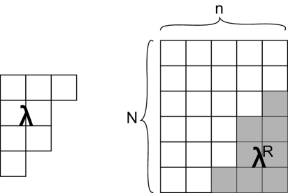
Figure 3: The Young tableau for $n^{N}/\lambda$, the shadowed part labeled as $\lambda^{R}$ has been cut out from $n^{N}$.

Proposition 1.

Given a Jack bra state of the rectangular graph,

$$|p_{-N,-n}\rangle_{\{n^{N}\}}=J_{-n^{N}}|p_{-N,-n}\rangle,$$

if it is acted from the left by a Jack annihilation operator $J_{\lambda}$, $\lambda\prec n^{N}$, $J_{n^{N}/\lambda}|p_{-N,-n}\rangle:=J_{\lambda}(\frac{a}{k})|p_{-N,-n}\rangle_{\{n^{N}\}}$, then $J_{n^{N}/\lambda}|p_{-N,-n}\rangle$ is again a Jack bra state up to a normalization constant.

$$J_{\lambda}(\frac{a}{k})|p_{-N,-n}\rangle_{\{n^{N}\}}\propto|p_{-N,-n}\rangle_{\{n^{N}/\lambda\}}.$$

Here, the introducing of $p_{-N,-n}$ for the oscillator vacuum state is artificial. It just make the comparison with the “Virasoro” null vector easier. The Young tableau $\{n^{N}\}/\lambda$ is shown in fig.3. Before rushing to the proof of the proposition, we start from some simple examples according to the level of the graphs being cut.

4.1.1 Example 0: level 0

In order to show that

$$|p_{-N,-n}\rangle_{\{n^{N}\}}\propto|\chi_{N,n}\rangle\,,$$ (52)

we just have to calculate

$$\hat{H}|\chi_{N,n}\rangle = (N\beta+\beta-1-\alpha_{+}\tilde{a}_{0})\tilde{a}_{-n}\tilde{a}_{n}|\chi_{N,n}\rangle$$

$$= Nn^{2}|\chi_{N,n}\rangle$$

Notice that $E_{n^{N}}=Nn^{2}$, eq.(52) is proved.

4.1.2 Example 1: level 1

Level one graph is just a single square. If we cut a square in the SE corner of the rectangular graph, the resulting state is proportional to

$$\tilde{a}_{1}J_{n^{N}}|p_{-N,-n}\rangle.$$

It is easy to show that the ”Virasoro part” of the Hamiltonian have eigenvalue on the resulting state

$$\alpha_{+}\tilde{a}_{-n}\tilde{L}_{n}\tilde{a}_{1}|p_{-N,-n}\rangle_{\{n^{N}\}}=((N-1)\beta-(n-1))\tilde{a}_{1}|p_{-N,-n}\rangle_{\{n^{N}\}},$$

And the diagonal part of $\hat{H}$ has the eigenvalue

$$(\beta N+\beta-1-\alpha_{+}\tilde{a}_{0})(nN-1)\tilde{a}_{1}|p_{-N,-n}\rangle_{\{n^{N}\}}=n(nN-1)\tilde{a}_{1}|p_{-N,-n}\rangle_{\{n^{N}\}}.$$

Combining the two parts together, we have

$$\hat{H}\tilde{a}_{1}|p_{-N,-n}\rangle_{\{n^{N}\}}=E_{n^{N}/\Box}\tilde{a}_{1}|p_{-N,-n}\rangle_{\{n^{N}\}},$$

Again this state has the correct property corresponding to the skew Young tableau $\{n^{N}/\Box\}$.

4.1.3 Example 2: level 2

There are two different Young tableaux $\lambda^{(1)}$ and $\lambda^{(2)}$ at level 2. If we cut these Young tableaux from a rectangular one $s^{r}$, the resulting states will span a two dimensional Hilbert space. Let us denote them as

$$|\chi\rangle=(\frac{\tilde{a}_{1}^{2}}{2k^{2}}+A\tilde{a}_{2})|\psi\rangle_{\{n^{N}\}},$$

here $A$ is an undetermined parameter. Note that the “diagonal part” of the Hamiltonian only shift the eigenvalue by a global constant. So for the eigen-equation

$$\hat{H}|\chi\rangle=E_{\chi}|\chi\rangle.$$

we can drop this diagonal term and consider only the ”Virasoro part” of the Hamiltonian. After a simple computation, one finds

$$A=\frac{1}{\sqrt{2}k^{3}}\,\,\,\text{or}\,\,\,\frac{-1}{\sqrt{2}k}$$

corresponding to $\lambda^{(1)}=\{2\}$ and $\lambda^{(2)}=\{1^{2}\}$ respectively.

4.1.4 Example 3: level 3

It is straightforward to continue on to level 3 graphs being cut. The resulting state is denoted as

$$|\chi\rangle=(\frac{\tilde{a}_{1}^{3}}{2\sqrt{2}k^{3}})+A\tilde{a}_{1}\tilde{a}_{2}+B\tilde{a}_{3}|\psi\rangle_{\{n^{N}\}},$$

here $A,B$ are undetermined parameters. There are three independent solutions for the eigen-equation corresponds to the three Young tableau at level 3.

For the horizontal Young tableau $\{3,0\}$, one gets : $A=3/2k^{4},\,\,\,\,B=\sqrt{2}/k^{5}.$

For the vertical Young tableau $\{1,1,1\}$, $A=-3/2k^{4},\,\,\,\,B=\sqrt{2}/k^{2}.$

For the symmetric Young tableau $\{2,1\}$, $A=-\frac{1}{2k^{2}}(1-\frac{1}{k^{2}}),\,\,\,\,B=\frac{-1}{\sqrt{2}k^{3}}.$

These results reproduce the level 3 Jack polynomials.

4.2 Proof by Brute Force Operator Formalism

Having checked for the low level skew Jack states, we are encouraged to find a more general proof for the proposition 1. In this section, we shall show that if $\langle J_{\lambda}|$ is a Jack symmetric function related to Young tableau $\lambda$, then $J_{\lambda}|\chi_{r,s}\rangle$ is proportional to a Jack symmetric function related to a Young tableau $s^{r}/\lambda$, with $\lambda\prec s^{r}$. Here, $|\chi_{r,s}\rangle$ is a Virasoro singular vector descendant from $|p_{-r,-s}\rangle$, see eq.(49). We can prove this in operator formalism first by “brute force”. Later in the next section we shall present it in a more compact manner. To proceed, we need to write the operator valued Jack function as follows:

$$J_{\lambda}=\sum_{\lambda^{\prime},|\lambda^{\prime}|=|\lambda|}C_{\lambda}^{\lambda^{\prime}}a_{\lambda^{\prime}_{1}}\cdots a_{\lambda_{s}^{\prime}}\,.$$ (54)

Then consider the commutator of $J_{\lambda}$ and $\hat{H}$ defined in eq.(22),

$$[J_{\lambda},\hat{H}] = \sum_{\lambda^{\prime},l}C_{\lambda}^{\lambda^{\prime}}a_{\lambda_{1}^{\prime}}\cdots[a_{\lambda^{\prime}_{l}},\hat{H}]\cdots a_{\lambda^{\prime}_{s}}$$

$$= \sum_{\lambda^{\prime},l}C_{\lambda}^{\lambda^{\prime}}a_{\lambda_{1}^{\prime}}\cdots[(1-\beta)(\lambda^{\prime}_{l})^{2}a_{\lambda^{\prime}_{l}}+2k\lambda^{\prime}_{l}L_{\lambda^{\prime}_{l}}^{\prime}+\beta Nla_{\lambda^{\prime}_{l}}]\cdots a_{\lambda_{s}^{\prime}}\,,$$

here

$$L^{\prime}_{l}=\frac{1}{2}\sum_{m\in Z}(:a_{m}a_{l-m}:)-a_{0}a_{l}\,.$$

In deriving this, we have used the commutation between $a_{l}$ and $\hat{H}$:

$$[a_{l},\hat{H}] = (1-\beta)l^{2}a_{l}+\sum_{m>0}2kla_{-m}a_{l+m}+\sum_{l>m>0}kla_{l-m}a_{m}+\beta Nla_{l}$$

$$= (1-\beta)l^{2}a_{l}+2klL^{\prime}_{l}+\beta Nla_{l}\,.$$

In moving $L_{\lambda^{\prime}_{l}}^{\prime}$ to the most left by the commutation relation $[L^{\prime}_{n},a_{m}]=-ma_{m+n}$ for $n,m>0$, more terms are generated,

$$[J_{\lambda},\hat{H}] = \sum_{\lambda^{\prime},l}C_{\lambda}^{\lambda^{\prime}}a_{\lambda_{1}^{\prime}}\cdots a_{\lambda^{\prime}_{l-1}}[(1-\beta)(\lambda^{\prime}_{l})^{2}a_{\lambda^{\prime}_{l}}+\beta N\lambda^{\prime}_{l}a_{\lambda^{\prime}_{l}}]\cdots a_{\lambda^{\prime}_{s}}$$

$$+ \sum_{\lambda^{\prime},n<l}C_{\lambda}^{\lambda^{\prime}}(2k\lambda^{\prime}_{l}\lambda^{\prime}_{n})a_{\lambda_{1}^{\prime}}\cdots a_{\lambda^{\prime}_{n}+\lambda^{\prime}_{l}}\cdots a_{\lambda^{\prime}_{l-1}}a_{\lambda^{\prime}_{l+1}}\cdots a_{\lambda_{s}^{\prime}}$$

$$+ \sum_{\lambda^{\prime},l}C_{\lambda}^{\lambda^{\prime}}(2k\lambda^{\prime}_{l})L_{\lambda_{l}^{\prime}}^{\prime}a_{\lambda_{1}^{\prime}}\cdots a_{\lambda_{l-1}^{\prime}}a_{\lambda^{\prime}_{l+1}}\cdots a_{\lambda^{\prime}_{s}}\,.$$

Let us define some notations to simplify our calculation. We denote the first line on the r.h.s. of eq.(4.2) as $A_{0}$ since this term retain the same number of $a_{n}$’s comparing to the original terms in $J_{\lambda}$, the second line is named as $A_{-}$ since it contains one less $a_{n}$ comparing to the original term in $J_{\lambda}$, the third line separates into two terms $A_{+}+\not{A}$, which are defined as

$$A_{+} = \sum_{\lambda^{\prime},l,\lambda^{\prime}_{l}>m>0}C_{\lambda}^{\lambda^{\prime}}k\lambda^{\prime}_{l}a_{\lambda_{1}^{\prime}}\cdots a_{\lambda_{l-1}^{\prime}}(a_{\lambda^{\prime}_{l}-m}a_{m})a_{\lambda^{\prime}_{l+1}}\cdots a_{\lambda^{\prime}_{s}}$$

$$\not{A} = \sum_{\lambda^{\prime},l,m>0}C_{\lambda}^{\lambda^{\prime}}(2k\lambda^{\prime}_{l})(a_{-m}a_{\lambda^{\prime}_{l}+m})a_{\lambda_{1}^{\prime}}\cdots a_{\lambda_{l-1}^{\prime}}a_{\lambda^{\prime}_{l+1}}\cdots a_{\lambda_{s}^{\prime}}\,.$$

If we apply eq.(4.2) to a bra vacuum sate $\langle{0}|$, the contribution of $\not{A}$ vanishes. Since $\langle{J_{\lambda}}|$ is an eigenstate of $\hat{H}$, we conclude

$$\langle{0}|J_{\lambda}\hat{H}=\langle{0}|J_{\lambda}E_{\lambda}\Rightarrow$$

$$\left[J_{\lambda},\hat{H}\right]=E_{\lambda}J_{\lambda}+\not{A}$$ (57)

$$E_{\lambda}J_{\lambda}=A_{+}+A_{-}+A_{0}$$ (58)

Now we calculate the action of $\hat{H}$ on the ket state $J_{\lambda}|{\chi_{r,s}}\rangle$

$$\hat{H}J_{\lambda}|{\chi_{r,s}}\rangle=[\hat{H},J_{\lambda}]|{\chi_{r,s}}\rangle+J_{\lambda}\hat{H}|{\chi_{r,s}}\rangle=[\hat{H},J_{\lambda}]|{\chi_{r,s}}\rangle+E_{rs}J_{\lambda}|{\chi_{r,s}}\rangle\,.$$ (59)

By moving $L_{\lambda_{l}}^{\prime}$ in eq.(4.2) to the most right, we get

$$[\hat{H},J_{\lambda}] = E_{\lambda}J_{\lambda}-2A_{+}-2A_{0}$$

$$- \sum_{\lambda^{\prime},l}(2k\lambda^{\prime}_{l})C_{\lambda}^{\lambda^{\prime}}a_{\lambda_{1}^{\prime}}\cdots a_{\lambda^{\prime}_{l-1}}a_{\lambda^{\prime}_{l+1}}\cdots a_{\lambda^{\prime}_{s}}\left[L_{\lambda^{\prime}_{l}}^{\prime}-\frac{1}{2}\sum_{\lambda^{\prime}_{l}>m>0}a_{\lambda^{\prime}_{l}-m}a_{m}\right]\,.$$

and

$$2A_{+}+2A_{0}+\sum_{\lambda^{\prime},l}(2k\lambda^{\prime}_{l})C_{\lambda}^{\lambda^{\prime}}a_{\lambda_{1}^{\prime}}\cdots a_{\lambda^{\prime}_{l-1}}a_{\lambda^{\prime}_{l+1}}\cdots a_{\lambda^{\prime}_{s}}\left[L_{\lambda^{\prime}_{l}}^{\prime}-\frac{1}{2}\sum_{\lambda^{\prime}_{l}>m>0}a_{\lambda^{\prime}_{l}-m}a_{m}\right]$$

$$= \sum_{\lambda^{\prime},l}2k\lambda^{\prime}_{l}C_{\lambda}^{\lambda^{\prime}}a_{\lambda_{1}^{\prime}}\cdots a_{\lambda^{\prime}_{l-1}}a_{\lambda^{\prime}_{l+1}}\cdots a_{\lambda^{\prime}_{s}}$$

$$\times [\sum_{m>0}(a_{-m}a_{\lambda^{\prime}_{l}+m})+\sum_{\lambda^{\prime}_{l}>m>0}(a_{\lambda^{\prime}_{l}-m}a_{m})+[-(k-\frac{1}{k})\lambda_{l}^{\prime}+Nk]a_{\lambda^{\prime}_{l}}]$$

$$= 2k(\sqrt{2}\alpha_{0}-\sqrt{2}\tilde{a}_{0})+Nk)|\lambda|J_{\lambda}+\sum_{\lambda^{\prime},l}2k\lambda^{\prime}_{l}C_{\lambda}^{\lambda^{\prime}}a_{\lambda_{1}^{\prime}}\cdots a_{\lambda^{\prime}_{l-1}}a_{\lambda^{\prime}_{l+1}}\cdots a_{\lambda^{\prime}_{s}}\tilde{L}_{\lambda^{\prime}_{l}}\,,$$

In deriving these, use has been made of eq.(58) and eq.(47). Substituting the results in eqs.(4.2-4.2) to eq.(59) and using the property of the Virasoro singular vector, $\tilde{L}_{l}|{\chi_{r,s}}\rangle=0,\,\,l>0$, we conclude

$$\hat{H}J_{\lambda}|{\chi_{r,s}}\rangle=\left[E_{\lambda}+E_{r,s}-|\lambda|\hat{M}\right]J_{\lambda}|{\chi_{r,s}}\rangle\,,$$ (62)

here

$$\hat{M}=2k(\sqrt{2}\alpha_{0}-\sqrt{2}\tilde{a_{0}}+Nk),$$

on $|{\chi_{r,s}}\rangle$, $\tilde{a_{0}}$ gives

$$\tilde{a}_{0}|{\chi_{r,s}}\rangle=\left(\dfrac{1+r}{2}\alpha_{+}+\dfrac{1+s}{2}\alpha_{-}\right)|{\chi_{r,s}}\rangle\,.$$ (63)

The establishment of eq.(62) finishes the proof of the proposition 1 we proposed before, that is, Jack polynomials for rectangular Young tableaux, skewed by an Jack state is again a Jack state.

4.3 More Compact Proof

The proposition 1 is proven in the previous subsection by making use of the eigen-equation for $\hat{H}$. However, we know that the eigenstate of $\hat{H}$ can always been written as an integral transformation,

$$\langle{J_{\lambda}}| \propto \langle{0}|\oint e^{k\sum_{n>0}\frac{a_{n}}{-n}p_{-n}}\prod_{i<j}|z_{i}-z_{j}|^{2\beta}J_{\lambda}(\{z_{i}\})\prod_{i}\dfrac{dz_{i}}{z_{i}}$$

$$\equiv \langle{0}|\oint F_{\lambda}(a,z)\prod_{i}\dfrac{dz_{i}}{z_{i}}\,.$$

Here $a\equiv\{a_{n}\}$, $z\equiv\{z_{i}\}$, and in the following the integration measure $\prod_{i}\dfrac{dz_{i}}{z_{i}}$ will be implied without written out explicitly. With $J_{\lambda}$ realized in this way, we found that the brute force proof can be rewritten in a more compact form with less indices involved. Using:

$$a_{-m}e^{k\sum_{n>0}\frac{a_{n}}{-n}p_{-n}}=e^{k\sum_{n>0}\frac{a_{n}}{-n}p_{-n}}(a_{-m}+kp_{-m})$$ (65)

$$e^{k\sum_{n>0}\frac{a_{n}}{-n}p_{-n}}a_{-m}=(a_{-m}-kp_{-m})e^{k\sum_{n>0}\frac{a_{n}}{-n}p_{-n}}\,,$$ (66)

we have

$$\int F_{\lambda}(a,z)\hat{H} = \int\left[\sum_{n,m=1}^{\infty}k\left((a_{-n}-kp_{-n})(a_{-m}-kp_{-m})a_{n+m}+(a_{-n-m}-kp_{-n-m})a_{n}a_{m}\right)\right.$$

$$+ \left.\sum_{n=1}^{\infty}(a_{-n}-kp_{-n})a_{n}(\beta N+n(1-\beta))\right]F_{\lambda}(a,z)$$

$$= \int\hat{H}F_{\lambda}(a,z)+\int\left[\sum_{n,m=1}^{\infty}(k^{3}p_{-n}p_{-m}a_{n+m}-2k^{2}p_{-m}a_{-n}a_{n+m}-k^{2}p_{-n-m}a_{n}a_{m})\right.$$

$$- \left.\sum_{n=1}^{\infty}kp_{-n}a_{n}(\beta N+n(1-\beta))\right]F_{\lambda}(a,z)\,.$$

Since the terms containing $a_{-n}$’s on the most left will annihilate the bra vacuum $\langle{0}|$, we conclude the following identity

$$\left[J_{\lambda},\hat{H}\right] = E_{\lambda}J_{\lambda}-\int 2k^{2}\sum_{n,m=1}^{\infty}p_{-m}a_{-n}a_{n+m}F_{\lambda}(a,z)$$ (68)

will be true. Comparing eq.(4.3) and eq.(68), we have

$$\int\left[\sum_{n,m=1}^{\infty}(k^{3}p_{-n}p_{-m}a_{n+m}-k^{2}p_{-n-m}a_{n}a_{m})\right.$$

$$- \left.\sum_{n=1}^{\infty}kp_{-n}a_{n}(\beta N+n(1-\beta))\right]F_{\lambda}(a,z)=E_{\lambda}J_{\lambda}\,.$$

Now we move $a_{-n}$’s in the last term in eq. (68) to the most right to get:

$$\left[J_{\lambda},\hat{H}\right]=E_{\lambda}J_{\lambda}-\int 2k^{2}\sum_{n,m=1}^{\infty}F_{\lambda}(a,z)p_{-m}(a_{-n}+kp_{-n})a_{n+m}\,.$$ (70)

Using eq.(4.3), the last term in the above eqation can be rewritten as

$$-2E_{\lambda}J_{\lambda}-\int F_{\lambda}(a,z)\left(\sum_{n,m=1}^{\infty}2k^{2}(p_{-m}a_{-n}a_{n+m}+p_{-n-m}a_{n}a_{m})\right.$$

$$+ \left.\sum_{n=1}^{\infty}2kp_{-n}a_{n}(\beta N+n(1-\beta))\right)\,,$$

Substituting this result into eq.(70), we have

$$\left[J_{\lambda},\hat{H}\right] = -E_{\lambda}J_{\lambda}-2k^{2}\int F_{\lambda}(a,z)\left\{\sum_{n,m=1}^{\infty}p_{-m}\left(\sum_{n=1}^{\infty}(a_{-n}a_{n+m})+\sum_{n=1}^{m-1}a_{n}a_{m-n}\right)\right.$$

$$+ \left.\sum_{m=1}^{\infty}p_{-m}a_{m}(kN+m(k^{-1}-k))\right\}$$

$$= -E_{\lambda}J_{\lambda}-2k^{2}\int F_{\lambda}(a,z)\left\{\sum_{m=1}^{\infty}p_{-m}(\tilde{L}_{m}+a_{m}(kN-(k^{-1}-k))-2a_{0})\right\}\,,$$

where $\tilde{L}_{m}$ is the same as what we defined in eq.(47). When we apply eq.(4.3) to a Virasoro singular vector $|{\chi_{rs}}\rangle$, $\tilde{L}_{n}|{\chi_{rs}}\rangle=0$ implies:

$$\left[\hat{H},J_{\lambda}\right]|{\chi_{rs}}\rangle=\left(E_{\lambda}J_{\lambda}+2k^{2}\int F_{\lambda}(a,z)\sum_{m>0}p_{-m}a_{m}(kN+(k-k^{-1})-2a_{0})\right)|{\chi_{rs}}\rangle\,.$$ (73)

Now we can check, using eqs.(4.3-65),

$$-k\int F_{\lambda}(a,z)\sum_{m>0}p_{-m}a_{m}=[J_{\lambda},\sum_{m>0}a_{-m}a_{m}]=|\lambda|J_{\lambda}\,,$$

which leads to

$$\hat{H}J_{\lambda}|{\chi_{rs}}\rangle=\left(E_{\lambda}+E_{\chi_{rs}}-2k|\lambda|(kN+k-k^{-1}-2a_{0})\right)J_{\lambda}|{\chi_{rs}}\rangle\,.$$ (74)

Here and before we have assumed that Virasoro $\tilde{L}_{n}$ singular state $|{\chi_{rs}}\rangle$ is an eigenstate for CS Hamiltonian $\hat{H}$ with eigenvalue $E_{\chi_{rs}}$. This can be checked as follows. From the formula, eq.(46)

$$H=k\sum_{n=1}^{\infty}a_{-n}\tilde{L}_{n}+\sum_{n=1}^{\infty}(\beta N+\beta-1-2ka_{0})a_{-n}a_{n}\,,$$

we arrive at: $E_{\chi_{rs}}=(\beta N+\beta-1-\sqrt{2}kp_{-r,-s})l$, here $l$ is the level of the decendant states. By the construction of Virasoro singular vectors, we know $l=rs,\,\,\sqrt{2}p_{-r,-s}=(1+r)k-(1+s)k^{-1}$, hence

$$E_{\chi_{rs}}=\left[\beta N+\beta-1-k((1+r)k-(1+s)\frac{1}{k})\right]|\lambda|$$ (75)

$$=rs^{2}+\beta(N-r)rs=E_{\{s^{r}\}}\,.$$

Thus eq.(73) implies that $J_{\lambda}|{\chi}\rangle$ is an eigenstate of $\hat{H}$ with the eigenvalue

$$E_{\lambda}+E_{s^{r}}-2k|\lambda|(kN+k-k^{-1}-(1+r)k+(1+s)k^{-1})$$

$$= E_{\lambda}+E_{s^{r}}-2|\lambda|((N-r)\beta+s))=E_{s^{r}/\lambda}\,.$$

This concludes our proof of proposition 1.

5 Skew-Recursive Construction of Jack States

In the previous sections we have shown that if we cut, inside a rectangular Young tableau of size $r\times s$, any sub-Young tableau in a skew way, the resulting Young tableau is unique and hence the corresponding Jack function, which is named as $J_{s^{r}/\lambda}$. This Jack function, $J_{s^{r}/\lambda}$, can be used again to cut another bigger rectangular Young tableau of size $r_{1}\times s_{1}$ to get $J_{s_{1}^{r_{1}}/(s^{r}/\lambda)}$ and so forth. If we know the construction of the Jack function for a definite Young tableau, we can build a tower of Jack functions upon it in such a skew way. Of course, if we start with a trivial Young tableau (empty), then the tower of Jack functions is built upon the constructions of the Jack function for rectangular Young tableau only, which are in fact Virasoro singular vectors. Following is the precise procedure which leads to the recursive construction of the Jack functions.

5.1 Operator Formalism

First, $J_{-\lambda}$ acts on the left vacuum to create a bra state

$${}_{\lambda}\langle{0}|\equiv\langle{0}|J_{\lambda},$$

$J_{\lambda}$ acts to the right will produce a skew ket state

$$J_{\lambda}|{0}\rangle_{\{s_{1}^{r_{1}}\}} \equiv J_{\lambda}J_{-s_{1}^{r_{1}}}|{0}\rangle\equiv J_{-s_{1}^{r_{1}}/\lambda}|{0}\rangle$$

$$= g_{\lambda,s_{1}^{r_{1}}/\lambda}^{s_{1}^{r_{1}}}j^{-1}_{[\lambda,s_{1}^{r_{1}}]}J_{-[\lambda,s_{1}^{r_{1}}]}|{0}\rangle$$

$$= g_{\lambda,s_{1}^{r_{1}}/\lambda}^{s_{1}^{r_{1}}}j^{-1}_{[\lambda,s_{1}^{r_{1}}]}|{0}\rangle_{\{s_{1}^{r_{1}}/\lambda\}}\,.$$

Here we use the symbol $[\lambda,s^{r}]$ to represent the unique Young tableau $s^{r}/\lambda$, see fig.3, where $\lambda^{R}$ means $\lambda$ rotated by $\pi$ angle. Such type of Young tableau, i.e., a rectangular one cut in the SE corner by a rotated $\lambda$, will be frequently used recursively. For example, $[[\lambda,s_{1}^{r_{1}}],s_{2}^{r_{2}}]$ will define another Jack function associated with the Young tableau $s_{2}^{r_{2}}$ cut in the SE corner by $[\lambda,s_{1}^{r_{1}}]$ rotated.

To facilitate such recursive procedure, we shall define the following abbreviation

$$[r,s]_{\lambda,n} \equiv \left[\cdots[[\lambda,s_{1}^{r_{1}}],s_{2}^{r_{2}}],\cdots,s_{n}^{r_{n}}\right]$$ (78)

$$\langle J_{(r,s)_{\lambda,n+1}} \equiv \langle J_{s_{n+1}^{r_{n+1}}}J_{-(r,s)_{\lambda,n}}\,,$$

$$J_{(r,s)_{\lambda,0}} = J_{\lambda}\,.$$

Here and after, however, we shall take $\lambda$ to be the empty Young tableau, so we shall use the abbreviation

$$[r,s]_{n} \equiv \left[\cdots[[s_{1}^{r_{1}},s_{2}^{r_{2}}],s_{3}^{r_{3}}],\cdots,s_{n}^{r_{n}}\right]$$ (79)

$$\langle{J_{(r,s)_{n+1}}}| \equiv \langle{J_{s_{n+1}^{r_{n+1}}}J_{-(r,s)_{n}}}|$$

$$J_{(r,s)_{0}} = 1\,.$$

It is clear that any regular Young tableau can be represented uniquely by two integer vectors of dimension $n$ each, $[r,s]_{n}$, where $n-1$ is the total number of skews for the Young tableau considered according to our convention. From the definition eq. (5.1), we know that $J_{(r,s)_{n}}$ differ from the standard Jack symmetric function $J_{[r,s]_{n}}$ only by a normalization constant. For example,

$$|J_{-(r,s)_{1}}\rangle = J_{-s_{1}^{r_{1}}}|{0}\rangle$$ (80)

$$\langle{J_{(r,s)_{2}}}| = \langle{0}|J_{s_{2}^{r_{2}}}J_{-s_{1}^{r_{1}}}\equiv\langle{0}|J_{s_{2}^{r_{2}}/s_{1}^{r_{1}}}$$

$$= g_{s_{1}^{r_{1}},s_{2}^{r_{2}}/s_{1}^{r_{1}}}^{s_{2}^{r_{2}}}j^{-1}_{s_{2}^{r_{2}}/s_{1}^{r_{1}}}\langle{0}|J_{[s_{1}^{r_{1}},s_{2}^{r_{2}}]}$$

$$J_{-(r,s)_{3}}|{0}\rangle = J_{(r,s)_{2}}J_{-s_{3}^{r_{3}}}|{0}\rangle$$

$$= g_{s_{1}^{r_{1}},s_{2}^{r_{2}}/s_{1}^{r_{1}}}^{s_{2}^{r_{2}}}j^{-1}_{[s_{1}^{r_{1}},s_{2}^{r_{2}}]}J_{[s_{1}^{r_{1}},s_{2}^{r_{2}}]}J_{-s_{3}^{r_{3}}}|{0}\rangle$$

$$= g_{s_{1}^{r_{1}},s_{2}^{r_{2}}/s_{1}^{r_{1}}}^{s_{2}^{r_{2}}}j^{-1}_{[s_{1}^{r_{1}},s_{2}^{r_{2}}]}g_{[s_{1}^{r_{1}},s_{2}^{r_{2}}],[[s_{1}^{r_{1}},s_{2}^{r_{2}}],s_{3}^{r_{3}}]}^{s_{3}^{r_{3}}}$$

$$\times j^{-1}_{[[s_{1}^{r_{1}},s_{2}^{r_{2}}],s_{3}^{r_{3}}]}J_{-[[s_{1}^{r_{1}},s_{2}^{r_{2}}],s_{3}^{r_{3}}]}|{0}\rangle$$

In general, the normalization constant can be determined as following. Suppose

$$J_{(r,s)_{n}}=C_{[r,s]_{n}}J_{[r,s]_{n}}\,,$$

then

$$\langle{J_{(r,s)_{n+1}}}| = \langle{0}|J_{s_{n+1}^{r_{n+1}}}J_{-(r,s)_{n}}=\langle{0}|J_{s_{n+1}^{r_{n+1}}}J_{-[r,s]_{n}}C_{[r,s]_{n}}$$

$$= g_{[r,s]_{n},[[r,s]_{n},s_{n+1}^{r_{n+1}}]}^{s_{n+1}^{r_{n+1}}}j^{-1}_{[[r,s]_{n},s_{n+1}^{r_{n+1}}]}\langle{J_{[r,s]_{n+1}}}|C_{[r,s]_{n+1}}\,,$$

so $C_{\lambda}$ can be defined recursively:

$$C_{[r,s]_{n+1}}=C_{[r,s]_{n}}g_{[r,s]_{n},[r,s]_{n+1}}^{s_{n+1}^{r_{n+1}}}j_{[r,s]_{n+1}}^{-1},$$ (84)

where the fusion coefficient $g_{[r,s]_{n},[r,s]_{n+1}}^{s_{n+1}^{r_{n+1}}}$ is calculated in eq.(2.5).

5.2 Integral Representation

In practice, an integral formalism is more useful in analysis. Based on the operator formalism, we derive the following integrals for building the Jack symmetric functions.

5.2.1 Auxiliary Scalar Fields

Since $J_{s^{r}}$’s are essentially the building blocks for any generic Jack function $J_{[r,s]_{n}}$, we come back to the construction of $J_{s^{r}}$ by the following integral,

$$J_{-s^{r}}|{p}\rangle = \int[dz]_{r}^{+}\prod_{i=1}^{r}z_{i}^{-s-1}e^{\sum_{n>0}\frac{a_{-n}p_{n}}{n}}|{p}\rangle\,,$$ (85)

here we have defined

$$[dz]_{r}^{+} \equiv \dfrac{B_{s^{r}}}{\Gamma_{r}^{2}}\prod_{i<j}|z_{i}-z_{j}|^{2\beta}\prod_{i=1}^{r}dz_{i}$$

$$\,[dz]_{s}^{-} \equiv \dfrac{(-1)^{sr}A_{s^{r}}}{\Gamma_{r}^{2}}\prod_{i<j}|z_{i}-z_{j}|^{2/\beta}\prod_{i=1}^{s}dz_{i}\,.$$

To relate $J_{-s^{r}}|{p}\rangle$ to a Virasoro singular vector, we introduce two scalar field, $\varphi^{(0)}$ and $\varphi^{(1)}$ to provide the right integration measure $[dz]$,

$$\langle\varphi^{(i)}(z)\varphi^{(j)}(z^{\prime})\rangle=\delta_{ij}\log(z-z^{\prime})\,,$$

and define the vertex operator integral

$$V_{01}^{\pm}=\oint:e^{k^{\pm 1}(\varphi^{(0)}+\varphi^{(1)})(z)}:\,\,\,\,.$$

Clearly, $V_{01}^{\pm}$ is the screening charge for the Virasoro algebra $L_{n}^{\pm}$ respectively. Here

$$T^{01,\pm}(z) \equiv \sum_{n\in\mathbb{Z}}L_{n}^{\pm}z^{-n-2}$$

$$= \frac{1}{4}(\partial_{z}(\varphi^{(0)}+\varphi^{(1)}))^{2}\pm\frac{1}{2}(k-\frac{1}{k})\partial^{2}_{z}(\varphi^{(0)}+\varphi^{(1)})\,.$$

Define

$$|{\chi_{rs}^{+}}\rangle = (V_{01}^{+})^{r}|{p_{r,-s}}\rangle$$

$$\langle{\chi^{-}_{rs}}| = \langle{p_{-r,s}}|(V_{01}^{-})^{s}\,,$$

clearly we have

$$L_{n}^{+}|{\chi_{rs}^{+}}\rangle=0,\,\,\,n>0$$

$$\langle{\chi_{rs}^{-}}|L_{-n}^{-}=0,\,\,\,n>0\,.$$

However, to get $J_{s^{r}}$, we have to project out one of the two scalar fields, say, $\varphi^{(0)}$ and from eq.(45) we get,

$$J_{s^{r}}(\dfrac{a^{(1)}_{-}}{k})|{p}\rangle_{1}\propto_{0}\langle{p}|\chi_{rs}^{+}\rangle$$ (86)

$${}_{1}\langle{p}|J_{s^{r}}(\dfrac{a^{(1)}}{k})\propto\langle{\chi_{rs}^{-}}|p\rangle_{0}\,,$$ (87)

so that now $J_{\pm s^{r}}$ contains only $a^{(1)}_{\pm n}$’s.

Now the Jack states read

$$|J_{-s^{r}}\rangle = \int\prod_{i=1}^{r}z_{i}^{-s-1}[dz]_{r}^{+}e^{k\sum_{n>0}\frac{a_{-n}^{(1)}p_{n}}{n}}|{p}\rangle_{1}\equiv J_{-(r,s)_{1}}\rangle$$ (88)

$$\langle J_{s^{r}}| = {}_{1}\langle{p}|\int e^{\frac{1}{k}\sum_{n>0}\frac{a_{n}^{(1)}p_{-n}}{-n}}\prod_{i=1}^{s}z_{i}^{r-1}[dz]_{s}^{-}\equiv\langle J_{(r,s)_{1}}\,,$$ (89)

here $|{p}\rangle_{i}$ is the vacuum state (no oscillator excitations) for the $\varphi^{(i)}$ scalar

$$a_{n}^{(i)}|{p}\rangle_{i}=\delta_{n,0}p^{(i)}|{p}\rangle_{i}\,\,\,\,n\geq 0$$ (90)

Notice that since $a_{-n}^{(0)}$ has been projected out, $J_{-s^{r}}$ is no longer a null vector for $L_{n}^{+}$. However, $J_{-s^{r}}$ is still a null vector for the modified Virasoro generator $\tilde{L}_{n}$ constructed with $\varphi^{(1)}$ only, see, eq. (47).

5.2.2 Bra and Ket States

Now we shall specify how the bra state $\langle{p^{+}_{p_{r,s}}}|$ and the ket state $|{p^{-}_{p_{r,s}}}\rangle$ are labeled.

Since we have $L_{n}^{\pm}$ acts on ket-state and bra-state respectively, so we have different screening charges for $L_{n}^{\pm}$ respectively.

$$\alpha^{++}=\sqrt{2}k,\,\,\,\alpha^{+-}=-\sqrt{2}k^{-1}$$

for $L_{n}^{+}$, and

$$\alpha^{-+}=-\sqrt{2}k,\alpha^{--}=\sqrt{2}k^{-1}$$

for $L_{n}^{-}$. If we combine $\varphi^{(i)}+\varphi^{(i+1)}$ into a single scalar,

$$\varphi=\dfrac{1}{\sqrt{2}}(\varphi^{(i)}+\varphi^{(i+1)}),$$

and

$$a_{0}|{p_{r,s}}\rangle = p^{+}_{r,s}|{p_{r,s}}\rangle$$

$$\langle{p_{r,s}}|a_{0} = \langle{p_{r,s}}|p^{-}_{rs}\,,$$

then we define

$$p^{+}_{rs} = \frac{1}{2}(1-r)\alpha^{++}+\frac{1}{2}(1-s)\alpha^{+-}$$

$$= \frac{1}{2}(1-r)\sqrt{2}k-\frac{1}{2}(1-s)\frac{\sqrt{2}}{k}$$

$$p_{rs}^{-} = \frac{1}{2}(1+r)\alpha^{-+}+\frac{1}{2}(1+s)\alpha^{--}$$

$$= -\frac{1}{2}(1+r)\sqrt{2}k+\frac{1}{2}(1+s)\frac{\sqrt{2}}{k}$$

Now consider

$$a_{0}|{p^{+}_{r,s}}\rangle_{i,i+1}=p^{+}_{r,s}|{p_{r,s}}\rangle_{i,i+1}\,.$$

However, when, say $\varphi^{(i)}$ is projected out, then

$$a_{0}^{(i+1)}|{p^{+}_{r,s}}\rangle_{i+1}=\dfrac{1}{\sqrt{2}}p^{+}_{r,s}|{p^{+}_{r,s}}\rangle_{i+1}\,.$$

For $\langle{p^{-}_{r,s}}|$, the projection is similar. To see this notation will provide the correct integration measure, one could check:

$$\langle{p^{-}_{-r,s}}|(V^{-})^{s}/\Gamma_{s}^{2}|{p^{+}_{-r,-s}}\rangle_{i}$$

$$= \langle{p^{-}_{-r,-s}}|\int\dfrac{\prod_{i<j}(z_{i}-z_{j})^{\frac{2}{k^{2}}}\prod_{i=1}^{s}z_{i}^{\frac{\sqrt{2}}{k}a_{0}}}{\Gamma_{s}^{2}}e^{\frac{\sqrt{2}}{k}\sum_{n>0}\frac{a_{n}}{-n}p_{-n}}\prod dz_{i}|{p^{+}_{-r,-s}}\rangle_{i}$$

$$= {}_{i+1}\langle{p^{-}_{-r,-s}}|\int\dfrac{\prod_{i<j}(z_{i}-z_{j})^{\frac{2}{k^{2}}}}{\Gamma_{s}^{2}}\prod_{i=1}^{s}z_{i}^{\frac{\sqrt{2}}{k}(\frac{1}{2}(1-r)(-\sqrt{2}k)+\frac{1}{2}(1-s)\frac{\sqrt{2}}{k})}e^{\frac{1}{k}\sum_{n>0}\frac{a^{(i+1)}_{n}}{-n}p_{-n}}\prod_{i}dz_{i}$$

$$= {}_{i+1}\langle{p^{-}_{-r,-s}}|\int\prod_{i<j}\left[\dfrac{(z_{i}-z_{j})^{2}}{z_{i}z_{j}}\right]^{\frac{1}{k^{2}}}e^{\frac{1}{k}\sum_{n>0}\frac{a^{(i+1)}_{n}}{-n}p_{-n}}\prod_{i=1}^{s}z_{i}^{r-1}dz_{i}/\Gamma_{s}^{2}$$

$$= {}_{i+1}\langle{\chi_{rs}}|\propto\langle{p^{-}_{-r,-s}}|\int e^{\frac{1}{k}\sum_{n>0}\frac{a^{(i+1)}_{n}}{-n}p_{-n}}\prod_{i=1}^{s}(z_{i})^{r-1}[dz]^{-}_{s}$$

$$= {}_{i+1}\langle{p^{-}_{-r,-s}}|J_{s^{r}}(\frac{a^{(i+1)}}{k})\,,$$

produces the Jack states of rectangular graph.

5.2.3 Integral Recursion

Now we have

$$|{J_{-s_{1}^{r_{1}}}}\rangle = |{J_{-(r,s)_{1}}}\rangle=\,\,_{0}\langle{p_{0}}|{\chi_{r_{1},s_{1}}}\rangle_{01}$$

$$= \int e^{\sum_{n>0}\frac{a_{-n}^{(1)}p_{n}}{n}k}\prod_{i=1}^{r_{1}}(z_{1,i})^{-s-1}[dz_{1}]_{r_{1}}^{+}|{p^{+}_{-r_{1},-s_{1}}}\rangle_{1}$$

$$p_{0} = \frac{1}{\sqrt{2}}p^{+}_{-r_{1},-s_{1}}=\frac{1}{2}(1+r_{1})k-\frac{1}{2}(1+s_{1})\frac{1}{k}\,.$$

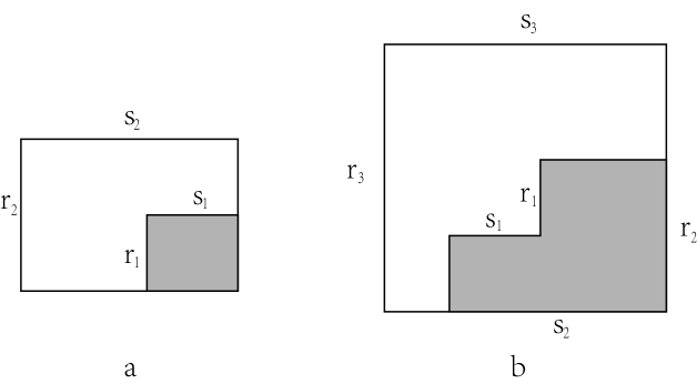
Figure 4: a. Young tableau $\{s_{2}^{r_{2}}\}/\{s_{1}^{r_{1}}\}$    b. Young tableau $\{s_{3}^{r_{3}}\}/(\{s_{2}^{r_{2}}\}/\{s_{1}^{r_{1}}\})$, this is a three-ladder Young tableau.

For one skew Young tableau of the type as in fig.4.a, we have to introduce $\varphi^{(2)}$ scalar and project out $\varphi^{(1)}$ scalar. The resulting state is actually the skew Jack state, as what has been shown in eq.(45); We proceed to construct

$$\langle{J_{(r,s)_{2}}}| = {}_{12}\langle{\chi_{r_{2},s_{2}}}|e^{\delta k_{21}q}J_{-(r,s)_{1}}|p^{+}_{-r_{1},-s_{1}}\rangle_{1}$$

$$= {}_{12}\langle{p^{-}_{-r_{2},-s_{2}}}|(V_{12}^{-})^{s_{2}}e^{\delta k_{21}q^{(1)}}J_{-{(r,s)_{1}}}|p^{+}_{-r_{1},-s_{1}}\rangle_{1}$$

$$= {}_{2}\langle{p^{-}_{-r_{2},-s_{2}}}|\iint e^{\sum{n>0}\frac{1}{k}\frac{a_{n_{2}}^{(2)}\sum z_{2,i}^{-n_{2}}}{-n_{2}}}\prod_{i=1}^{s_{2}}(z_{2,i})^{r_{2}-1}\prod_{s_{2},r_{1}}(1-\frac{z_{1}}{z_{2}})\prod_{i=1}^{r_{1}}(z_{1,i})^{-s_{1}-1}[dz_{2}]_{s_{2}}^{-}[dz_{1}]^{+}_{r_{1}}\,.$$

Here we have defined

$$\prod^{s_{m},r_{n}}(1-\frac{z_{n}}{z_{m}})\equiv\prod_{i=1}^{s_{m}}\prod_{j=1}^{r_{n}}(1-\frac{z_{n,j}}{z_{m,i}})\,.$$

and $e^{\delta k_{21}q}$ is introduced to eliminate the charge deficit in $\varphi^{(1)}$ sector, that is

$${}_{1}\langle{p^{-}_{-r_{2},-s_{2}}}|e^{\delta k_{21}q^{(1)}}|{p^{+}_{-r_{1},-s_{1}}}\rangle_{1}\neq 0\,.$$ (96)

will give the following equation,

$$\dfrac{1}{\sqrt{2}}p^{-}_{-r_{2},-s_{2}} = \delta k_{21}+\frac{1}{\sqrt{2}}p^{+}_{-r_{1},-s_{1}}$$ (97)

$$\delta k_{21} = (p^{-}_{-r_{2},-s_{2}}-p^{+}_{-r_{1},-s_{1}})\dfrac{1}{\sqrt{2}}$$

$$= \frac{1}{2}(\frac{1}{k}-k)-\frac{k}{2}(1+r_{1}-r_{2})+\frac{1}{2k}(1+s_{1}-s_{2})$$

$$= \dfrac{1}{\sqrt{2}}\left\{\alpha_{0}^{-}+p^{+}_{r_{1}-r_{2},s_{1}-s_{2}}\right\}$$

$$2\alpha_{0}^{\pm} = \alpha^{\pm+}+\alpha^{\pm-}\,.$$

For two skew Young tableau,fig.4.b, $\varphi^{(3)}$ is introduced and $\varphi^{(2)}$ eliminated.

$$|{J_{-(r,s)_{3}}}\rangle = {}_{2}\langle p^{-}_{-r_{2},-s_{2}}|J_{(r,s)_{2}}e^{\delta k_{23}q^{(2)}}|{\chi_{r_{3},s_{3}}}\rangle_{23}$$

$$= {}_{2}\langle p^{-}_{-r_{2},-s_{2}}|J_{(r,s)_{2}}|e^{\delta k_{23}q^{(2)}}(V_{2}^{+})^{r_{3}}|{p^{+}_{-r_{3},-s_{3}}}\rangle_{23}$$

$$= \int\prod_{i=1}^{r_{3}}(z_{3,i})^{-s_{3}-1}[dz_{3}]_{r_{3}}^{+}\prod^{s_{2},r_{3}}\left(1-\frac{z_{3}}{z_{2}}\right)\prod_{i=1}^{s_{2}}(z_{2,i})^{r_{2}-1}[dz_{2}]_{s_{2}}^{-}$$

$$\times \prod^{s_{2},r_{1}}\left(1-\frac{z_{1}}{z_{2}}\right)\prod_{i=1}^{r_{1}}(z_{1,i})^{-s_{1}-1}[dz_{1}]_{r_{1}}^{+}\exp\left(k\sum_{n>0}\frac{a_{-n}^{(3)}}{n}\sum_{i}z_{3,i}^{n}\right)|{p^{+}_{-r_{3},-s_{3}}}\rangle_{3}$$

Similarly, we have

$$\delta k_{23}+\frac{1}{\sqrt{2}}p^{+}_{-r_{3},-s_{3}} = \frac{1}{\sqrt{2}}p^{-}_{-r_{2},-s_{2}}$$ (100)

$$\delta k_{23} = \frac{1}{\sqrt{2}}(-\alpha_{0}^{+}-p^{+}_{r_{2}-r_{3},s_{2}-s_{3}})=\frac{1}{\sqrt{2}}(\alpha_{0}^{-}+p^{-}_{r_{3}-r_{2},s_{3}-s_{2}})$$

$$= \frac{1}{2}(\frac{1}{k}-k)-\frac{k}{2}(1+r_{3}-r_{2})+\frac{1}{2k}(1+s_{3}-s_{2})\,.$$

In general, proceed recursively, we have, for $n$ odd

$$J_{-(r,s)_{n}}|{p^{+}_{-r_{n},-s_{n}}}\rangle_{n} = {}_{n-1}\langle p^{-}_{-r_{n-1},-s_{n-1}}|J_{(r,s)_{n-1}}e^{\delta k_{n-1,n}q^{(n-1)}}|{\chi_{r_{n},s_{n}}}\rangle_{n-1,n}$$

$$= \iiint\exp\left({k\sum_{m>0}\dfrac{a_{-m}^{(n)}\sum_{i=1}^{r_{n}}z_{n,i}^{m}}{m}}\right)\prod_{i=1}^{r_{n}}(z_{n,i})^{-s_{n}-1}\prod^{s_{n-1},r_{n}}(1-\frac{z_{n}}{z_{n-1}})$$

$$\times \prod_{i=1}^{s_{n-1}}(z_{n-1,i})^{r_{n-1}-1}\prod^{s_{n-1},r_{n-2}}(1-\frac{z_{n-2}}{z_{n-1}})\cdots\prod_{i=1}^{s_{2}}(z_{2,i})^{r_{2}-1}$$

$$\times \prod^{s_{2},r_{1}}(1-\frac{z_{1}}{z_{2}})\prod_{i=1}^{r_{1}}(z_{1,i})^{-s_{1}-1}[dz]^{o}_{[n]!}|{p^{+}_{-r_{n},-s_{n}}}\rangle_{n}\,.$$

Here

$$\delta k_{n-1,n} = \frac{1}{\sqrt{2}}\left(-\alpha_{0}^{+}-p^{+}_{r_{n-1}-r_{n},s_{n-1}-s_{n}}\right)$$

$$= \frac{1}{\sqrt{2}}\left(\alpha_{0}^{-}+p^{-}_{r_{n}-r_{n-1},s_{n}-s_{n-1}}\right)$$

$$= \frac{1}{2}(\frac{1}{k}-k)-\frac{k}{2}(1+r_{n}-r_{n-1})+\frac{1}{2k}(1+s_{n}-s_{n-1})\,.$$

For $n$ even,

$${}_{n}\langle{p^{-}_{-r_{n},-s_{n}}}|J_{(r,s)_{n}} = \langle{\chi_{r_{n},s_{n}}}|e^{\delta k_{n,n-1}q^{(n-1)}}J_{-{(r,s)_{n-1}}}|p^{+}_{-r_{n-1},-s_{n-1}}\rangle_{n-1}$$

$$= {}_{n}\langle{p^{-}_{-r_{n},-s_{n}}}|\iiint\exp\left({\dfrac{1}{k}\sum_{m>0}\dfrac{a_{m}^{(n)}\sum_{i=1}^{s_{n}}z_{n,i}^{-m}}{-m}}\right)\prod_{i=1}^{s_{n}}(z_{n,i})^{r_{n}-1}\prod^{s_{n},r_{n-1}}(1-\frac{z_{n-1}}{z_{n}})$$

$$\times \prod_{i=1}^{r_{n-1}}(z_{n-1,i})^{-s_{n-1}-1}\prod^{s_{n-2},r_{n-1}}(1-\frac{z_{n-2}}{z_{n-1}})\cdots\prod_{i=1}^{s_{2}}(z_{2,i})^{r_{2}-1}$$

$$\times \prod^{s_{2},r_{1}}(1-\frac{z_{1}}{z_{2}})\prod_{i=1}^{r_{1}}(z_{1,i})^{-s_{1}-1}[dz]^{e}_{[n]!}\,.$$

Here,

$$\delta k_{n,n-1} = \frac{1}{\sqrt{2}}\left(-\alpha_{0}^{+}-p^{+}_{r_{n}-r_{n-1},s_{n}-s_{n-1}}\right)$$

$$= \frac{1}{\sqrt{2}}(\alpha_{0}^{-}+p^{-}_{r_{n-1}-r_{n},s_{n-1}-s_{n}})$$

$$= \frac{1}{2}(\frac{1}{k}-k)-\frac{k}{2}(1+r_{n-1}-r_{n})+\frac{1}{2k}(1+s_{n-1}-s_{n})\,.$$

The integration measures are defined as following: for $n$ odd,

$$[dz]_{[n]!}^{o}\equiv[dz_{1}]_{r_{1}}^{+}[dz_{2}]_{s_{2}}^{-}\cdots[dz_{n}]_{r_{n}}^{+}\,.$$

For $n$ even,

$$[dz]_{[n]!}^{e}\equiv[dz_{1}]_{r_{1}}^{+}[dz_{2}]_{s_{2}}^{-}\cdots[dz_{n}]_{s_{n}}^{-}\,.$$

Eq.(5.2.3) and eq.(5.2.3) are the main results of our present work. It provides an integral representation for any Jack symmetric function which, in our formalism, is labeled by two integer vectors of dimension $n$ each, $(r,s)_{n}$.

The integral representation not only provide a useful tool in analyzing problems involving Jack symmetric functions, but also give an explicit construction of the Jack symmetric functions in terms of free bosons. It is also desirable to work out explicitly the Selberg type multi-integrals appearing in eq.(5.2.3) and eq.(5.2.3).

5.3 Integral Representation for Jack Symmetric Polynomials

Having got the integral representation for a general Jack symmetric function, it is then straightforward to get the Jack symmetric polynomials in any number $N$ of arguments $z_{i}$. Notice that in the following we shall present the unnormalized Jack polynomials. However, the normalization constants can be easily worked out.

First, let us consider $n$ even, thus

$$J_{(r,s)_{n}}^{1/k^{2}}(\{z_{i}\}) \equiv \langle J_{(r,s)_{n}}\exp\left(k\sum_{m>0}\frac{a_{-m}^{(n)}}{m}\sum_{i=1}^{N}z_{i}^{m}\right)|{p^{+}_{n}}\rangle_{n}$$

$$= \iiint\prod^{s_{n},N}(1-\frac{z}{z_{n}})\prod_{i=1}^{s_{n}}(z_{n,i})^{r_{n}-1}[dz_{n}]_{s_{n}}^{-}\prod^{s_{n},r_{n-1}}(1-\frac{z_{n-1}}{z_{n}})\prod_{i=1}^{r_{n-1}}(z_{n-1,i})^{-s_{n-1}-1}[dz_{n-1}]_{r_{n-1}}^{+}$$

$$\times \prod^{s_{n-2},r_{n-1}}(1-\frac{z_{n-1}}{z_{n-2}})\prod_{i=1}^{s_{n-2}}(z_{n-2,i})^{r_{n-2}-1}[dz_{n-2}]_{s_{n-2}}^{-}\cdots$$

$$\times \prod^{s_{2},r_{1}}(1-\frac{z_{1}}{z_{2}})\prod_{i=1}^{r_{1}}(z_{1,i})^{-s_{1}-1}[dz_{i}]_{r_{1}}^{+}\,.$$

And for $n$ odd,

$$J^{1/k^{2}}_{(r,s)_{n}}(\{z_{i}^{-1}\}) \equiv {}_{n}\langle{p_{n}^{-}}|\exp\left(\frac{1}{k}\sum_{m>0}\frac{a_{m}^{(n)}}{-m}\sum_{i=1}^{N}z_{i}^{-m}\right)J_{-(r,s)_{n}}\rangle$$

$$= \iiint\prod^{N,r_{n}}(1-\frac{z_{n}}{z})\prod_{i=1}^{r_{n}}(z_{n,i})^{-s_{n}-1}[dz_{n}]_{r_{n}}^{+}\prod^{s_{n-1},r_{n}}(1-\frac{z_{n}}{z_{n-1}})\prod_{i=1}^{s_{n-1}}(z_{n-1,i})^{r_{n-1}-1}[dz_{n-1}]^{-}_{s_{n-1}}$$

$$\times \prod^{s_{n-1},r_{n-2}}(1-\frac{z_{n-2}}{z_{n-1}})\prod_{i=1}^{r_{n-2}}(z_{n-2,i})^{-s_{n-2}-1}[dz_{n-2}]^{+}_{s_{n-2}}\cdots$$

$$\times \prod^{s_{2},r_{1}}(1-\frac{z_{1}}{z_{2}})\prod_{i=1}^{r_{1}}(z_{1,i})^{-s_{1}-1}[dz_{1}]_{r_{1}}^{+}\,.$$

Now $p_{n}^{\pm}$ can be easily worked out,

$$p^{+}_{n} = \frac{1}{\sqrt{2}}p^{-}_{-r_{n},-s_{n}}=\frac{1}{\sqrt{2}}\left(\frac{1}{2}(1-r_{n})\alpha^{-+}+\frac{1}{2}(1-s_{n})\alpha^{--}\right)$$

$$= -\frac{k}{2}(1-r_{n})+\frac{1}{2k}(1-s_{n})$$

$$p^{-}_{n} = \frac{1}{\sqrt{2}}p^{+}_{-r_{n},-s_{n}}=\frac{k}{2}(1+r_{n})-\frac{1}{2k}(1+s_{n})\,.$$ (108)

6 Acknowledgement

This work is part of the CAS program ”Frontier Topics in Mathematical Physics” (KJCX3-SYW-S03) and is supported partially by a national grant NSFC(11035008).

References

- [1] H. Awata, Y. Matsuo, S. Odake and J. Shiraishi, “Excited states of Calogero-Sutherland model and singular vectors of the W(N) algebra,” Nucl. Phys. B 449, 347 (1995) [arXiv:hep-th/9503043].
- [2] H. Awata, Y. Matsuo, S. Odake and J. Shiraishi, “A Note on Calogero-Sutherland model, W(n) singular vectors and generalized matrix models,” Soryushiron Kenkyu 91, A69 (1995) [arXiv:hep-th/9503028].
- [3] H. Awata, M. Fukuma, Y. Matsuo and S. Odake, “Representation theory of W(1+infinity) algebra,”
- [4] H. Awata, Y. Matsuo, S. Odake and J. Shiraishi, “Collective field theory, Calogero-Sutherland model and generalized matrix models,” Phys. Lett. B 347, 49 (1995) [arXiv:hep-th/9411053].
- [5] T. H. Baker, P. J. Forrester, “The Calogero-Sutherland Model and Generalized Classical Polynomials” Commun. Math. Phys. 188, 175 216 (1997)
- [6] S. Iso and S. J. Rey, “Collective field theory of the fractional quantum hall edge state and the Calogero-Sutherland model,” Phys. Lett. B 352, 111 (1995) [arXiv:hep-th/9406192].
- [7] H. Azuma and S. Iso, “Explicit relation of quantum hall effect and Calogero-Sutherland model,” Phys. Lett. B 331, 107 (1994) [arXiv:hep-th/9312001].
- [8] Al. B. Zamolodchikov, “Conformal symmetry in two-dimensional space: Recursion representation of conformal block, Teoret. Mat. Fiz., 73:1 (1987), 103-110
- [9] Al. B. Zamolodchikov, “Conformal symmetry in two dimensions: An explicit recurrence formula for the conformal partial wave amplitude”, Commun. Math. Phys. 96, 3, 419-422,
- [10] K. Mimachi and Y. Yamada ,“Singular vectors of the Virasoro algebra in terms of Jack symmetric polynomials”, Comm. Math. Phys. 174, 2 (1995), 447-455 (1984)
- [11] Ha, Z. N. C. 1995, “Fractional statistics in one dimension: view from an exactly solvable model” Nuclear Physics B, 435, 604
- [12] Bernevig, B. A. and Haldane, F. D. M., “Model Fractional Quantum Hall States and Jack Polynomials”, Physical Review Letters, 2008, 100, 24, arXiv: 0707.3637
- [13] A. Okounkov and G. Olshanki “Shifted Jack Polynomials, Binomial Formula, and Applications” Mathematical Research Letters 4, 69-78 (1997)
- [14] L. Lapointe, & L. Vinet, 1995, “Exact operator solution of the Calogero-Sutherland model”, arXiv:q-alg/9509003
- [15] A. P. Polychronakos, “Exchange operator formalism for integrable systems of particles,” Phys. Rev. Lett. 69, 703 (1992) [arXiv:hep-th/9202057].
- [16] R. Sakamoto, J. Shiraishi, D. Arnaudon, L. Frappat and E. Ragoucy, “Correspondence between conformal field theory and Calogero-Sutherland model,” Nucl. Phys. B 704, 490 (2005) [arXiv:hep-th/0407267].
- [17] K. W. J. Kadell, “An integral for the product of two Selberg-Jack symmetric polynomials” ,Compositio Mathematica, 87 no. 1 (1993), p. 5-43
- [18] K. W. J. Kadell, “The Selberg-Jack Symmetric Functions ”, Advances in Mathematics 130, 1997, 33-102
- [19] R. P. Stanley, “Some Combinatorial Properties of Jack Symmetric Functions”, Advances in Mathematics 77, 76-115, (1989)
- [20] V. S. Dotsenko and V. A. Fateev, “Four Point Correlation Functions and the Operator Algebra in the Two-Dimensional Conformal Invariant Theories with the Central Charge ,” Nucl. Phys. B 251, 691 (1985).
- [21] B. L. Feigin and D. B. Fuks, “Invariant skew symmetric differential operators on the line and verma modules over the Virasoro algebra,” Funct. Anal. Appl. 16, 114 (1982) [Funkt. Anal. Pril. 16, 47 (1982)].
- [22] G. Felder, “BRST Approach to Minimal Methods,” Nucl. Phys. B317, 215 (1989).
- [23] V. A. Alba, V. A. Fateev, A. V. Litvinov and G. M. Tarnopolsky, “On combinatorial expansion of the conformal blocks arising from AGT conjecture,” arXiv:1012.1312 [hep-th].
- [24] L. F. Alday, D. Gaiotto and Y. Tachikawa, “Liouville Correlation Functions from Four-dimensional Gauge Theories,” Lett. Math. Phys. 91, 167 (2010) [arXiv:0906.3219 [hep-th]].
- [25] R. Dijkgraaf and C. Vafa, “Toda Theories, Matrix Models, Topological Strings, and N=2 Gauge Systems,” arXiv:0909.2453 [hep-th].
- [26] A. Belavin and V. Belavin, “AGT conjecture and Integrable structure of Conformal field theory for c=1,” Nucl. Phys. B 850, 199 (2011) [arXiv:1102.0343 [hep-th]].
- [27] N. A. Nekrasov and S. L. Shatashvili, “Quantization of Integrable Systems and Four Dimensional Gauge Theories,” arXiv:0908.4052 [hep-th].
- [28] E. Carlsson and A. Okounkov, “Exts and Vertex Operators,” arXiv: 0801.2565v2.
- [29] R. Donagi and E. Witten, “Supersymmetric Yang-Mills theory and integrable systems,” Nucl. Phys. B 460, 299 (1996) [arXiv:hep-th/9510101].
- [30] B. Shou, J. F. Wu and M. Yu, “AGT conjecture and AFLT states: A complete construction”, to appear.
- [31] J. F. Wu, Y. Y. Xu and M. Yu, in preparation.
- [32] I. G. Macdonald, Symmetric Functions and Hall Polynomials, 1995, 2nd Edition, Clarendon Press Oxford