Effects of density dependence of the effective pairing interaction on the first $2^{+}$ excitations and quadrupole moments of odd nuclei

Abstract

Excitation energies and transition probabilities of the first $2^{+}$ excitations in even tin and lead isotopes as well as the quadrupole moments of odd neighbors of these isotopes are calculated within the self-consistent Theory of Finite Fermi Systems based on the Energy Density Functional by Fayans et al. The effect of the density dependence of the effective pairing interaction is analyzed in detail by comparing results obtained with volume and surface pairing. The effect is found to be noticeable. For example, the $2^{+}$-energies are systematically higher at 200-300 keV for the volume paring as compared with the surface pairing case. But on the average both models reasonably agree with the data. Quadrupole moments of odd-neutron nuclei are very sensitive to the single-particle energy of the state $\lambda$ under consideration due to the Bogolyubov factor ($u^{2}_{\lambda}-v^{2}_{\lambda}$). A reasonable agreement with experiment for the quadrupole moments has been obtained for the most part of odd nuclei considered. The method used gives a reliable possibility to predict quadrupole moments of unstable odd nuclei including very neutron rich ones.

I Introduction

Presently there are two theoretical approaches which can quantitatively describe the bulk properties of nuclear isotope chains with a small number of effective coupling constants: selfconsistent mean field theories and density-functional theory. The successes and open problems of the mean field approaches are reviewed in Refs. REL-REV ; SHF-REV1 ; SHF-REV2 . The Kohn-Sham density functional theory was originally proposed for chemistry and solids KS ; Jones . Important theoretical developments have been made: an extension of the Hohenberg-Kohn theorem to pairing degrees of freedom by Oliveira, Gross, and Kohn allowed studies of superfluids oliveira and the generalization of functional theory to study excited states made it possible to investigate the electromagnetic response of correlated electron materials basov . In nuclear physics, a self-consistent Theory of Finite Fermi Systems (TFFS) was derived by Khodel and Saperstein KhS on the basis of the TFFS by Migdal AB supplemented with the many-body theory self-consistency relation Fay-Khod for the nucleon mass operator. As it was shown in Kh-Sap-Zv , the self-consistent TFFS for nuclei without pairing can be reformulated as a particular version of the density functional method with a rather complicated $\rho$-dependence of the energy functional. It contains also $\tau$-dependent terms but with rather small strength resulting for the effective mass in a small difference of $|m^{*}_{n,p}(r)-m|\simeq 0.05m$. In a series of articles by Fayans et al. STF ; Fay5 , (see also Fay and Refs. therein) the energy density functional (EDF) method was generalized for superfluid nuclei. Just as in the original Kohn–Sham approach, the identity $m^{*}=m$ was imposed. A fractional form of the density dependence for the central part of the normal component of the EDF was introduced. The coordinate dependence of it resembled that of Kh-Sap-Zv but the functional form was much simpler making the self-consistent QRPA calculations easier. Note that a recent generalization of the Skyrme force in EKR contains a new term with a density dependence resembling that in Fay . In addition, the velocity dependent force in EKR is rather weak leading to the effective mass $m^{*}\simeq 0.9m$. Thus, the selfconsistent mean field approaches may eventually converge with the density functional methods.

The non-relativistic versions of the self-consistent mean field theories introduce three-nucleon forces which are often expressed as a density dependent two-body interaction. In general, one assumes a fractional power of the density dependence. Recent advances in Effective Field Theory open the possibility to connect the density functional with the effective two- and three- nucleon systems which are determined from two-nucleon scattering and few-nucleon reactions. Reviews about the current status of such attempts are given in Refs.Epelbaum:2008ga ; Drut:2009ce .

The question arises whether the pairing interaction should have an analogous dependence on the normal nuclear density. Several studies derived pairing interactions from free two-nucleon interactions. Baldo et al. solved the gap equation in semi-infinite nuclear matter Bald1 , nuclear slab Bald2 , and finite nuclei Bald3 ; Bald4 . The Paris and Argonne v₁₈ $NN$ potentials were used, results being almost identical. To make results more appropriate for practical nuclear self-consistent calculations dealing with pairing in a model space, the pairing problem was treated in a two-step way. The gap equation was solved in a model space with limiting energy $E_{0}=30\div 40\;$MeV with the use of the effective pairing interaction. The latter is found in the subsidiary sub-space in terms of a free $NN$ potential. For all systems under consideration and the two $NN$ potentials the effective pairing interaction found is much stronger, up to ten times, at the surface than inside. The Milan group concentrated on the ¹²⁴Sn nucleus, a traditional benchmark for the nuclear pairing problem, and solved the gap equation starting from the Argonne v₁₄ potential milan1 . In addition to the free $NN$ interaction, they included corrections due to exchange with low-lying surface vibrations (“phonons”) milan2 and high-lying excitations, mainly spin-dependent ones, milan3 . In the last article, a local 3-parameter density-dependent effective pairing interaction is constructed for the model space with $E_{0}=60\;$MeV which reproduce approximately exact gap values. Qualitatively, it is similar to that described above. Without all corrections, it consists of a strong surface attraction and very weak attraction inside. Taking into account of the phonon exchange makes the inner interaction repulsive. At last, inclusion of the spin-dependent excitations makes the inner repulsion rather strong. Thus, the ab initio calculations of the effective pairing interaction predict essential density dependence with strong surface attraction.

As an alternative to consideration of the gap equation with complete realistic $NN$ interactions, Bulgac and Yu used the fact that this equation depends mainly on the low-$k$ behavior of $NN$ force which can be approximated with a rather simple analytical function. It helped to develop a renormalization scheme for the gap equation without any cutoff in terms of zero-range interactions with explicit coordinate dependence of the effective pairing interaction and to suggest an EDF for superfluid nuclei Bulgac1 ; Bulgac2 .

The calculations by Fayans et al. employed both volume pairing and surface pairing interactions. The binding energies and the proton and neutron separation energies were found to be insensitive to the type of pairing force used. But the odd-even staggering of charge radii can be quantitatively reproduced only if the strong density dependence of the pairing force is introduced Fay .

In this work, we investigate the excitation energies and transition rates of the low-lying $2^{+}$-states in spherical nuclei with the aim to analyze the sensitivity of those observables to the details of the pairing interaction. We will compare two opposite limits, the “volume pairing” with density independent effective pairing interaction ${\cal F}^{\xi}$ and the case of the function ${\cal F}^{\xi}$ with the surface dominance. The latter will be named for brevity the “surface pairing”. Several sets of calculations of these characteristics of the first $2^{+}$-excitations were carried out recently within the QRPA method with Skyrme force Bertsch1 ; Vor and within the Generator Coordinate Method with the Gogny force Bertsch2 . No systematic analysis of the density dependence of the pairing force was performed in these studies. Dealing with low-laying quadrupole excitations, it is natural to include into analysis also quadrupole moments of odd nuclei which give test of static quadrupole polarization.

In this paper, we use the EDF method Fay with the functional DF3-a Tol-Sap . In the latter the spin-orbit and effective tensor terms of the original functional DF3 Fay5 ; Fay were modified. All the QRPA-like TFFS equations are solved in the self-consistent basis $(\varepsilon_{\lambda},\varphi_{\lambda})$ obtained within the EDF method with the functional DF3-a.

II Brief outline of the formalism

For completeness, we describe shortly the EDF method of Fay using mainly the notation of Fay3 . In this method, the ground state energy of a nucleus is considered as a functional of normal and anomalous densities,

$$E_{0}=\int{\cal E}[\rho_{n}({\bf r}),\rho_{p}({\bf r}),\nu_{n}({\bf r}),\nu_{p}({\bf r})]d^{3}r.$$ (1)

The normal part of the EDF ${\cal E}_{\rm norm}$ contains the central, spin-orbit and effective tensor nuclear terms and Coulomb interaction term for protons. The main, central force, term of ${\cal E}_{\rm norm}$ is finite range with Yukawa-type coordinate dependence. It is convenient to extract the $\delta({\bf r}-{\bf r}^{\prime})$-term from the Yukawa function separating the rest of

$$D({\bf r}-{\bf r}^{\prime})=\frac{1}{4\pi r_{\rm c}^{2}|{\bf r}-{\bf r}^{\prime}|}\exp{\left(-\frac{|{\bf r}-{\bf r}^{\prime}|}{r_{\rm c}}\right)}-\delta({\bf r}-{\bf r}^{\prime})$$ (2)

to generate the “surface” part ${\cal E}^{\rm s}$ which vanishes in infinite matter with $\rho({\bf r})=const$. The Yukawa radius $r_{\rm c}$ is taken the same for the isoscalar and isovector channels. The “volume” part of the EDF, ${\cal E}^{\rm v}(\rho)$, is taken in Fay5 ; Fay ; Fay3 as a fractional function of densities $\rho_{+}=\rho_{n}+\rho_{p}$ and $\rho_{-}=\rho_{n}-\rho_{p}$:

$${\cal E}^{\rm v}(\rho)=C_{0}\left[a^{\rm v}_{+}\frac{\rho_{+}^{2}}{2}f^{\rm v}_{+}(x)+a^{\rm v}_{-}\frac{\rho_{-}^{2}}{2}f^{\rm v}_{-}(x)\right],$$ (3)

where

$$f^{\rm v}_{\pm}(x)=\frac{1-h^{\rm v}_{1\pm}x}{1+h^{\rm v}_{2\pm}x}.$$ (4)

Here $x=\rho_{+}/(2\rho_{0})$ is the dimensionless nuclear density where $\rho_{0}$ is the density of nucleons of one kind in equilibrium symmetric nuclear matter. The factor $C_{0}=(dn/d\varepsilon_{\rm F})^{-1}$ in Eq. (3) is the usual TFFS normalization factor, inverse density of states at the Fermi surface.

To write down the surface term in a compact form similar to (3), the “tilde” operator was introduced in Fay3 denoting the following folding procedure:

$$\widetilde{\phi({\bf r})}=\int D({\bf r}-{\bf r}^{\prime})\phi({\bf r^{\prime}})d{\bf r^{\prime}}.$$ (5)

Then we obtain

$${\cal E}^{\rm s}(\rho)=C_{0}\frac{1}{2}\left[a^{\rm s}_{+}(\rho_{+}f^{\rm s}_{+})\widetilde{(f^{\rm s}_{+}\rho_{+})}+a^{\rm s}_{-}(\rho_{-}f^{\rm s}_{-})\widetilde{(f^{\rm s}_{-}\rho_{-})}\right],$$ (6)

where

$$f^{\rm s}_{\pm}(x)=\frac{1}{1+h^{\rm s}_{\pm}x}.$$ (7)

All the above parameters, $a^{\rm v}_{\pm},a^{\rm s}_{\pm},h^{\rm v}_{1\pm}h^{\rm v}_{2\pm},h^{\rm s}_{\pm}$, are dimensionless.

In the momentum space, the operator (2) reads

$$D(q)=-\frac{(qr_{\rm c})^{2}}{1+(qr_{\rm c})^{2}}.$$ (8)

In the small $r_{\rm c}$ limit it reduces to $D(q)=-(qr_{\rm c})^{2}$, and Eq. (6) could be simplified to a Skyrme-like form proportional to $(\nabla\rho)^{2}$.

The spin-orbit interaction reads

$${\cal F}_{sl}=C_{0}r_{0}^{2}(\kappa+\kappa^{\prime}{\bm{\tau}}_{1}{\bm{\tau}}_{2})\left[\nabla_{1}\delta({\bf r}_{1}-{\bf r}_{2})\times({\bf p}_{1}-{\bf p}_{2})\right]\cdot({\bm{\sigma}}_{1}+{\bm{\sigma}}_{2}),$$ (9)

where the factor $r_{0}^{2}$ is introduced to make the spin-orbit parameters $\kappa,\kappa^{\prime}$ dimensionless. It can be expressed in terms of the above equilibrium density, $r_{0}^{2}=(3/(8\pi\rho_{0}))^{2/3}$.

In nuclei with partially occupied spin-orbit doublets, the so-called spin-orbit density exists,

$$\rho_{sl}^{\tau}(\bf r)=\sum_{\lambda}n_{\lambda}^{\tau}\langle\phi_{\lambda}^{\tau*}(\bf r)({\bm{\sigma}}{\bf l})\phi_{\lambda}^{\tau}(\bf r)\rangle,$$ (10)

where $\tau=n,p$ — is the isotopic index and averaging over spin variables is carried out. As it is well known, see e.g. KhS , a new term appears in the spin-orbit mean field induced by the tensor forces and the first harmonic $\hat{g_{1}}$ of the spin Landau–Migdal (LM) amplitude. We combine those contributions into an effective tensor force or first spin harmonic,

$${\cal F}_{1}^{s}=C_{0}r_{0}^{2}(g_{1}+g^{\prime}_{1}{\bm{\tau}}_{1}{\bm{\tau}}_{2})\delta({\bf r}_{1}-{\bf r}_{2})({\bm{\sigma}}_{1}{\bm{\sigma}}_{2})({\bf p}_{1}{\bf p}_{2}).$$ (11)

In Table 1, we present all parameters of the normal part of the EDF DF3-a we use. Note that the major part of these parameters is identical to the ones used in the DF3 functional Fay . With one exception, all parameters for the central force part remained the same and only the spin-orbit and the first spin harmonic are changed according Tol-Sap . Application of the volume part (3) to equilibrium nuclear matter, with the equilibrium relation, i.e. vanishing pressure $p(\rho)=\rho^{2}\partial({\cal E}/\rho)/\partial\rho$, permits to find the parameters $a^{\rm v}_{+},h^{\rm v}_{1+}$ and $h^{\rm v}_{2+}$ in terms of the nuclear matter density $\rho_{0}$, the chemical potential $\mu_{0}$, and the compression modulus $K_{0}=9dp/d\rho$. The asymmetry energy parameter $\beta_{0}$ yields a relation between the constants $a^{\rm v}_{-},h^{\rm v}_{1-}$ and $h^{\rm v}_{2-}$. They are given in the upper half of Table 1. The radius $r_{0}$ introduced above is shown instead of $\rho_{0}$. The value used in Ref. Fay was recalibrated in Ref. Tol-Sap to obtain a more accurate description of nuclear charge radii Sap-Tol . One more remark should be made concerning the table. The “natural” TFFS normalizing factor $C_{0}=2\varepsilon_{0\rm F}/(3\rho_{0})=308.2\;$MeV fm³ corresponding to parameters of nuclear matter in the third column of the table differs from the one, $C_{0}=300\;$MeV fm³, recommended in the second edition of the Migdal’s textbook on the TFFS AB2 . To make a comparison with other articles within the TFFS, we recalculated all the strength parameters to the latter. It explains a small difference of some values in the second column in the table from the original those in Fay . An essential difference between DF3 and DF3-a functionals takes place for the “spin-dependent” sector in the bottom of the table. As we found in Tol-Sap , the second one describes the spin-orbit splitting of doublets better.

The anomalous component of the EDF Fay reads

$${\cal E}_{\rm an}({\bf r})=\sum_{\tau}{\cal F}^{\xi,\tau\tau}({\bf r};[\rho])|\nu^{\tau}({\bf r})|^{2},$$ (12)

where the effective pairing interaction reads:

$${\cal F}^{\xi}=C_{0}f^{\xi}=C_{0}\left(f^{\xi}_{\rm ex}+h^{\xi}x^{2/3}+f^{\xi}_{\nabla}r_{0}^{2}(\nabla x)^{2}\right).$$ (13)

The first two terms are similar to those in the TFFS Sap-Tr ; Zv-Sap2 or in the SHFB method Gor1 . The third in (13) is a new one introduced in Fay5 . In this paper we use an approximate version of (13) with $f^{\xi}_{\nabla}=0$. We will compare two models for nuclear pairing: the “volume” pairing ($h^{\xi}=0$) and the “surface” pairing where both the pairing parameters $f^{\xi}_{\rm ex}$ and $h^{\xi}$ are nonzero. One more remark should be made concerning the pairing problem. In the approach Fay pairing was considered in the coordinate representation explicitly, solving the Gorkov equations with the method developed in Ref. Bel . However, it was found that the results are practically equivalent to those obtained within a more simple BCS-like scheme using the gap $\Delta_{\lambda\lambda^{\prime}}=\Delta_{\lambda}\delta_{\lambda\lambda^{\prime}}$ in a sufficiently large model space, $\varepsilon_{\lambda}<E_{\rm max}$. The effective pairing interaction (13) for the BCS approximation is a little stronger than that in the coordinate representation (at $\simeq 5\div 10$%, depending on $E_{\rm max}$). For the systematic calculations in this article we use this simplified method of considering the pairing problem with $E_{\rm max}=36\;$MeV. We do not apply this method for nuclei close to the dripline for which the diagonal approximation doesn’t work Fay .

Table 1: Parameters of the normal part of the EDF

Parameter	DF3 Fay	DF3-a Tol-Sap
$\mu_{0},\;$MeV	-16.05	-16.05
$r_{0},\;$fm	1.147	1.145
$K_{0},\;$MeV	200	200
$\beta,\;$MeV	28.7	28.7
$a^{\rm v}_{+}$	-6.598	-6.575
$h^{\rm v}_{1+}$	0.163	0.163
$h^{\rm v}_{2+}$	0.724	0.725
$a^{\rm v}_{-}$	5.565	5.523
$h^{\rm v}_{1-}$	0	0
$h^{\rm v}_{2-}$	3.0	3.0
$a^{\rm s}_{+}$	-11.4	-11.1
$h^{\rm s}_{+}$	0.31	0.31
$a^{\rm s}_{-}$	-4.11	-4.10
$h^{\rm s}_{-}$	0	0
$r_{\rm c},\;$fm	0.35	0.35
$\kappa$	0.216	0.190
$\kappa^{\prime}$	0.077	0.077
$g_{1}$	0	0
$g_{1}^{\prime}$	-0.123	-0.308

Within the TFFS, the response of a nucleus to the external quadrupole field $V_{0}\exp{(i\omega t)}$ can be found in terms of the effective field. In systems with pairing correlations, equation for the effective field can be written in a compact form as

$${\hat{V}}(\omega)={\hat{V}}_{0}(\omega)+{\hat{\cal F}}{\hat{A}}(\omega){\hat{V}}(\omega),$$ (14)

where all the terms are matrices. In the standard TFFS notation AB , we have:

$${\hat{V}}=\left(\begin{array}[]{c}V\\ d_{1}\\ d_{2}\end{array}\right)\,,\quad{\hat{V}}_{0}=\left(\begin{array}[]{c}V_{0}\\ 0\\ 0\end{array}\right)\,,$$ (15)

$${\hat{\cal F}}=\left(\begin{array}[]{ccc}{\cal F}&{\cal F}^{\omega\xi}&{\cal F}^{\omega\xi}\\ {\cal F}^{\xi\omega}&{\cal F}^{\xi}&{\cal F}^{\xi\omega}\\ {\cal F}^{\xi\omega}&{\cal F}^{\xi\omega}&{\cal F}^{\xi}\end{array}\right),$$ (16)

$${\hat{A}}(\omega)=\left(\begin{array}[]{ccc}{\cal L}(\omega)&{\cal M}_{1}(\omega)&{\cal M}_{2}(\omega)\\ {\cal O}(\omega)&-{\cal N}_{1}(\omega)&{\cal N}_{2}(\omega)\\ {\cal O}(-\omega)&-{\cal N}_{1}(-\omega)&{\cal N}_{2}(-\omega)\end{array}\right)\,,$$ (17)

where ${\cal L},\;{\cal M}_{1}$, and so on stand for integrals over $\varepsilon$ of the products of different combinations of the Green function $G(\varepsilon)$ and two Gor’kov functios $F^{(1)}(\varepsilon)$ and $F^{(2)}(\varepsilon)$. They can be found in AB and we write down here only the first of them which is of the main importance for us,

$${\cal L}=\int\frac{d\varepsilon}{2\pi i}\left[G(\varepsilon)G(\varepsilon+\omega)-F^{(1)}(\varepsilon)F^{(2)}(\varepsilon+\omega)\right].$$ (18)

Isotopic indices in Eqs. (15-17) are omitted for brevity. In Eq. (16), ${\cal F}$ is the usual LM amplitude,

$${\cal F}=\frac{\delta^{2}{\cal E}}{\delta\rho^{2}},$$ (19)

whereas the amplitudes ${\cal F}^{\omega\xi}={\cal F}^{\xi\omega}$ stand for the mixed second derivatives,

$${\cal F}^{\omega\xi}=\frac{\delta^{2}{\cal E}}{\delta\rho\delta\nu}.$$ (20)

In the case of volume pairing, we have ${\cal F}^{\omega\xi}=0$. The explicit form of the above equations and (18) is written down for the case of the electric ($t$-even) symmetry we deal with. A static moment of an odd nucleus can be found in terms of the diagonal matrix element $\langle\lambda_{0}|V(\omega=0)|\lambda_{0}\rangle$ of the effective field over the state $\lambda_{0}$ of the odd nucleon.

The effective field operator ${\hat{V}}(\omega)$ has a pole in the excitation energy $\omega_{s}$ of the state $|s\rangle$ under consideration,

$${\hat{V}}(\omega)=\frac{\left({\hat{V}_{0}}{\hat{A}(\omega_{s})}{\hat{g}}_{0s}\right){\hat{g}}_{0s}}{\omega-\omega_{s}}+{\hat{V}}_{R}(\omega).$$ (21)

The quantity ${\hat{g}}_{0s}$ has the meaning of the corresponding excitation amplitude. It obeys the homogeneous counterpart of Eq. (14) and is normalized as follows AB ,

$$\left({\hat{g}}_{0s}^{+}\frac{d{\hat{A}}}{d\omega}{\hat{g}}_{0s}\right)_{\omega=\omega_{s}}=-1,$$ (22)

with obvious notation.

For excitation probabilities, it is more convenient to use the transition density operator which is conjugated to ${\hat{g}}_{0s}$,

$${\hat{\rho}}^{\rm tr}_{0s}={\hat{A}}{\hat{g}}_{0s}.$$ (23)

The explicit definition of the normal and anomalous components of ${\hat{\rho}}^{\rm tr}_{0s}$ is as follows

$$\rho^{{\rm tr}(0)}_{0s}({\bf r},{\bf r}^{\prime})=\int\frac{d\varepsilon}{2\pi i}\delta G({\bf r},{\bf r}^{\prime};\varepsilon,\omega_{s}),$$ (24)

$$\rho^{{\rm tr}(1,2)}_{0s}({\bf r},{\bf r}^{\prime})=\int\frac{d\varepsilon}{2\pi i}\delta F^{(1,2)}({\bf r},{\bf r}^{\prime};\varepsilon,\omega_{s}).$$ (25)

The TFFS equation for transition densities for nuclei with pairing correlations,

$${\hat{\rho}}^{\rm tr}_{0s}={\hat{A}}(\omega_{s}){\hat{\cal F}}{\hat{\rho}}^{\rm tr}_{0s},$$ (26)

is a complete analogue of the QRPA set of equations. Therefore we will often name it the QRPA equation. The transition density is normalized due to Eq. (22), and the transition matrix element for the excitation of the state $|s\rangle$ with the external field $V_{0}$ is given by

$$M_{0s}=\int{\hat{V}}_{0}{\hat{\rho}}^{\rm tr}_{0s}({\bf r})d{\bf r}.$$ (27)

III Characteristics of the $2^{+}_{1}$ excitations

The formalism described in the previous Section was used to describe $2^{+}_{1}$ states in two isotopic chains of semi-magic nuclei, lead and tin. We investigate both a pure surface and a pure volume version of pairing. More calculational details can be found in Ref. Fay . We use the so-called developed pairing approximation. In particular, we don’t make any corrections to particle non-conservation effects induced with the Bogolyubov transformation. Therefore in the vicinity of double magic nuclei, the results should be considered as very approximate. As it was found in Fay , it is impossible to describe neutron and proton separation energies $S_{n}$ and $S_{p}$ for all nuclei, from calcium up to lead, with sufficient accuracy using a fixed set of parameters in Eq. (13), the effective strength of the pairing interaction should be diminished with increasing nucleon number A.

Figure 1: (Color online) Neutron separation energies $S_{n}$ for lead isotopes. The volume pairing corresponds to ($f^{\xi}_{\rm ex}=-0.31;h^{\xi}=0$), the surface one, to ($f^{\xi}_{\rm ex}=-1.05;\;h^{\xi}=0.94$). The HFB theory predictions with the HFB-17 Skyrme functional are taken from site .

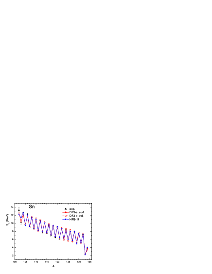
Figure 2: (Color online) Neutron separation energies $S_{n}$ for tin isotopes. The volume pairing corresponds to ($f^{\xi}_{\rm ex}=-0.33;\;h^{\xi}=0$), the surface one, to ($f^{\xi}_{\rm ex}=-1.05;\;h^{\xi}=0.92$). The HFB theory predictions with the HFB-17 Skyrme functional are taken from site .

In this paper, we limit ourselves to two long isotopic chains, the lead and the tin chains. Therefore we deal with neutron pairing only. A short comment should be made on the procedure of solving the pairing problem. No particle number projection procedure is used in our calculations, i.e. particle number is conserved only on average, corresponding to the chosen chemical potential $\mu$ for the kind of nucleons under consideration. The accuracy of this approximation is examined in a lot of papers. For the self-consistent SHF method with the SLy4 force, it was found in recent article part-numb that the average difference between exact and approximate gap values is 0.12 MeV, the error being bigger in vicinity of magic nuclei.

For finding the parameters of the pairing force (13) we use the strategy of “soft” variation of them to obtain better values of $S_{n}$ for both the chains under consideration. Values of $S_{n}$ for both kinds of pairing are compared with the data in Fig. 1 and Fig. 2. Explicit values of the pairing parameters are given in the figure captions. Remind that we use the two-parameter version of (13), with $f^{\xi}_{\nabla}=0$. For the volume pairing ($h^{\xi}=0$), one parameter remains which is smaller for lead than for tin approximately at 6%. For the surface pairing we deal with a two-parameter form of ${\cal F}^{\xi}$. The “external” pairing parameter $f^{\xi}_{\rm ex}$ is taken $A$-independent, in accordance with its physical meaning as the free NN $T$-matrix taken at negative energy $E=2\mu$ Bald1 . As to the second one, $h^{\xi}$, it increases from the Sn chain to the Pb one at 2%, the resulting pairing attraction again becoming weaker, but only a little. Thus, the $A$-independence of the pairing parameters in the case of surface pairing is weaker than for the volume one. This finding suggests to favor surface pairing. As we see, the difference between the predictions for neutron separation energies is small for both versions and agreement with the experimental data is nearly perfect. For comparison, we display the predictions of the HFB-17 version of the Skyrme force Gor1 which has a record accuracy in overall description of nuclear masses. We see that for these two chains our accuracy in description of neutron separation energies is even better. Of course, we achieved the agreement by a small variation of one of two paring parameters whereas calculations Gor1 are carried out with an universal set of parameters. However, the pairing part of the HFB-17 functional contains five parameters.

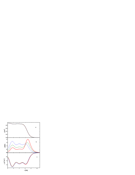
Figure 3: (Color online) Neutron density (pannel a), gap (b) and anomalous density (c) in ²⁰⁰Pb nucleus. Solid and dotted lines correspond to the surface and volume versions correspondingly, the dashed one, to the medium version ($f^{\xi}_{\rm ex}=-0.70;\;h^{\xi}=0.50$).

Fig. 3 demonstrates that the normal neutron density $\rho_{n}(r)$ and the anomalous one, $\nu_{n}(r)$, both are practically insensitive to the kind of paring used in the calculation. On the contrary, the gap itself is very sensitive. For comparison, we took also a “medium” version, with ($f^{\xi}_{\rm ex}=-0.70;\;h^{\xi}=0.50$). It gives $S_{n}$ value approximately with the same accuracy as the previous two.

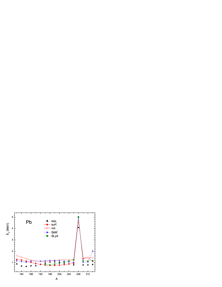
Figure 4: (Color online) Excitation energies $\omega(2^{+}_{1})$ for lead isotopes. Predictions for mean field approach with the forces SkM*(dashed blue line) and SLy4(dashed green line) are taken from Bertsch1 . The energy density functional results are given by the solid lines.

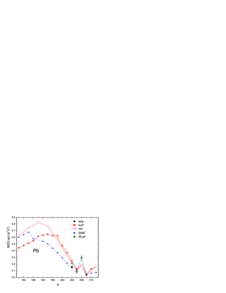
Figure 5: (Color online)$B(E2,{\rm up})$ values for lead isotopes. Predictions for the SkM* and SLy4 force are taken from Bertsch1 .

Let us now examine to what extent predictions for characteristics of $2^{+}_{1}$ states are different for these two versions of pairing force which are equivalent in describing the $S_{n}$ values. A comment should be made before presenting results of the QRPA calculations. Our QRPA code doesn’t include the spin-orbit (9) and spin (11) terms of the effective interaction, therefore the self-consistency is not complete and the excitation energy of the ghost $1^{-}$-state does not automatically vanish. In the present investigation, we fine tuned the parameter $a^{\rm v}_{+}$ in (3) in order to decouple the ghost state. This change is different for different nuclei but on average the value of $|a^{\rm v}_{+}|$ increases at $\simeq 3$% in comparison with that given in Table 1.

Let us begin with the lead chain. Excitation energies $\omega_{2}$ are displayed in Fig. 4 and the probabilities $B(E2,{\rm up})$, in Fig. 5. Experimental data for both quantities are taken from Dat . For comparison, results of the QRPA calculations of Bertsch1 with the SkM* and SLy4 force are shown. Note that they were carried out with density independent pairing. We see that the difference $\delta\omega_{2}=\omega_{2}^{\rm vol}-\omega_{2}^{\rm surf}$ is, on average, of the order of 0.3 MeV, that is the effect under discussion is noticeable for this quantity. The results for volume pairing are systematically higher, with the exception of the ^210,212Pb isotopes for which the two versions practically coincide. Agreement with the data is, on average, quite reasonable for both the versions. Predictions of both the SkM* and SLy4 QRPA calculations for $\omega_{2}$ values have approximately the same accuracy as ours.

For excitation probabilities the situation is more complex. For isotopes heavier than ¹⁹⁸Pb our “surface” and “volume” curves are very close to each other. For lighter part of the chain the volume pairing generates larger probabilities than surface pairing does, producing differences up to $\simeq 30$%. Comparing with Fig. 4, we see that there is some unusual correlation between excitations energies and probabilities. Indeed, in magic nuclei where the pairing is absent for low-lying collective excitations there is a rule that a lower energy implies a larger probability. It can be qualitatively explained with the hydrodynamical Bohr-Mottelson (BM) model BM2 which gives a simple relation for the transition density of a $L$-vibration:

$$\rho_{L}^{\rm tr,BM}=\alpha_{L}\frac{d\rho}{dr},$$ (28)

where $\alpha_{L}=1/\sqrt{2\omega_{L}B_{L}}$, and $B_{L}$ is the collective mass parameter of the BM model proportional to the nuclear mass. Then one obtains

$$B(EL,{\rm up})=\frac{2L+1}{2\omega_{L}B_{L}}(M_{L})^{2},$$ (29)

where $M_{L}^{\rm BM}=(3Ze/4\pi)R^{L-1}$, $R$ being the nuclear radius. Thus, in the BM model a lower value of the excitation energy $\omega_{L}$ inevitably leads to a higher value of the excitation probability. In our calculations, the situation is opposite. In principle, this is not strange. Indeed, even in magic nuclei the BM model works only qualitatively KhS . If one solves equations of the self-consistent TFFS or any HF+RPA equations for nuclei without pairing, Eq. (28) remains approximately true, but the mass parameter becomes $\omega$-dependent and deviates from the BM model prescription significantly KhS . In nuclei with pairing, the situation becomes even more different from this simplest model as the normal component of the transition density (24) depends now from the anomalous transition amplitudes ${\hat{g}}_{0s}^{(1,2)}$ (see Eq. (26)). They strongly depend on the kind of pairing. As a result, the correlation between the $\omega_{L}$ and $B(EL)$ values of the BM-type (29) can be destroyed.

Experimental probabilities are known only for four even ^204-210Pb isotopes. For all of them, the SkM* and SLy4 calculations are in perfect agreement with the data. Agreement of our calculations is poorer. It is especially true for the magic ²⁰⁸Pb nucleus where there is no any pairing. It should be noted that in this nucleus the collectivity of the $2^{+}_{1}$-state is not high: the B(E2) value is only about 8 single-particle units (spu). For a comparison, the B(E3) value for the $3^{-}_{1}$-state exceeds 30 spu. But for excitations with low collectivity in nuclei without pairing the RPA solution depends strongly on the single-particle spectrum, and even a small inaccuracy in the positions of single-particle levels can change results significantly. In any case, some modification of the normal part of the functional DF3-a is necessary to obtain better agreement for the ²⁰⁸Pb nucleus.

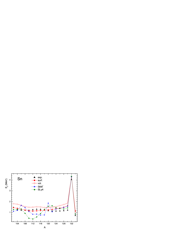
Figure 6: (Color online) Excitation energies $\omega(2^{+}_{1})$ for tin isotopes. Predictions for the SkM* and SLy4 force are taken from Bertsch1 .

In the tin chain, see Fig. 6, the situation with the excitation spectrum is partially similar to the one in lead. Again, $2^{+}_{1}$-levels are higher for volume pairing than in the surface case, and again the difference $\delta\omega_{2}$ is $\simeq 300\;$keV, the surface predictions being closer to the experimental data. As to the SkM* spectrum, for isotopes heavier than ¹²²Sn it practically coincides with our “surface” one, both being higher than the experimental spectrum by approximately $200\div 300\;$keV. For lighter isotopes, it deviates from our surface spectrum significantly in an irregular way whereas the latter practically coincides with the experiment in this $A$ region. As to the SLy4 spectrum, it also looks reasonable for the heavy part of the chain but for isotopes lighter of ¹²⁴Sn it strongly oscillates around the experimental curve. In the dip minimum for ¹¹²Sn the $\omega_{2}$ value is less than the experimental one at approximately 1 MeV and it is close to an instability.

The excitation probabilities are displayed in Fig. 7. Here the results show a very complex pattern. For the heavier part of the chain, beginning at the ¹²⁴Sn nucleus, our two theoretical curves and the SkM* practically coincide, all being close to the experiment. The SkM* curve behaves in a non-regular way with strong deviations from the experimental data, up to $\simeq 50\div 100$%. The Sly4 interaction produces excitation probabilities which strongly decrease with the nucleon number A, implying drastic deviations from the data. The density functional approach is able to describe the A-dependence of the experimental $B(E2,{\rm up})$ values rather well. For lighter tin isotopes, our two curves began to deviate from each other, the volume one being higher by $\simeq 25\div 30$%, and a first glance may suggest that the volume pairing interaction performs much better. On the other hand, one has to notice the large error bars of the experimental data in the mass region below A=114.

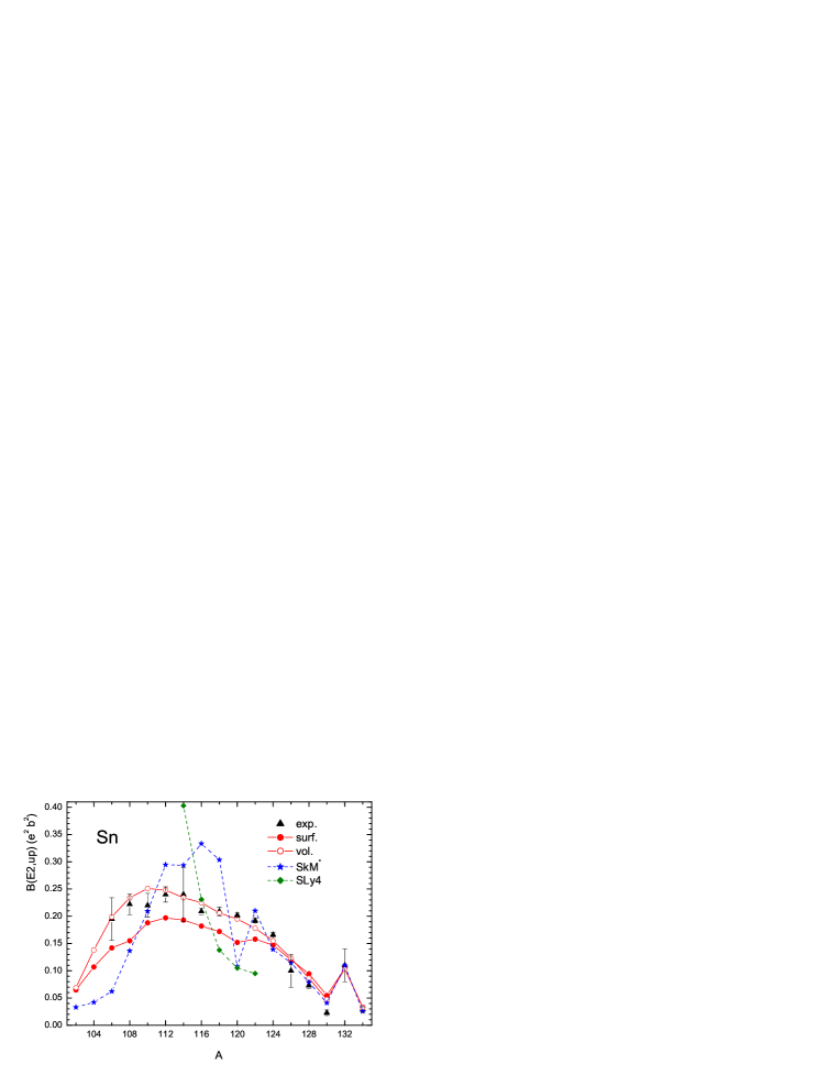
Figure 7: (Color online) $B(E2,{\rm up})$ values for tin isotopes. Predictions for the SkM* and SLy4 force are taken from Bertsch1 . Experimental data are taken for ^114-124Sn from Dat , for ^126-134Sn from newbe2 , and for ^106-112Sn from be2_106-112 ; be2_110 ; be2_106-108 .

To investigate the role of pairing itself and of the type of its density dependence in detail, let us analyze different components of the transition amplitude. Let us begin from the anomalous terms ${\hat{g}}^{(1,2)}$ (the index “0s” is for brevity omitted). They are displayed in Fig. 8 for the ²⁰⁰Pb nucleus. We see, first, that, for both the versions, the $g^{(1)}$ amplitude value is much bigger than $|g^{(2)}|$. Second, the coordinate dependence of the main $g^{(1)}$ amplitude is absolutely different for the two versions under comparison. In the surface pairing case, a strong surface maximum dominates whereas in the volume case $g^{(1)}$ is spread over the volume, with rather strong oscillations. In addition, it is seen that the integral effect of $g^{(1)}_{\rm surf}$ should be noticeably bigger than that of $g^{(1)}_{\rm vol}$. All this shows some asymmetry for Bogolyubov quasiparticles and quasiholes. Such a situation is typical for nuclei which are close to the magic core.

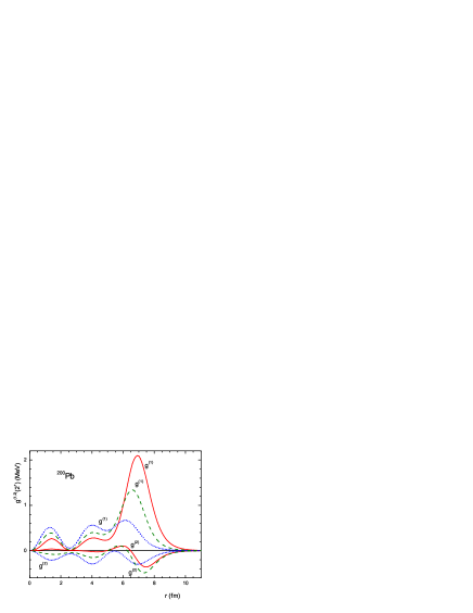
Figure 8: (Color online) The neutron anomalous transition amplitudes $g^{(1,2)}$ in ²⁰⁰Pb nucleus. Solid lines correspond to surface, dotted to volume, and dashed, to the medium kind of pairing, see Fig. 3.

The normal proton and neutron amplitudes $g^{(0)}$ for the same nucleus are displayed in Fig. 9. As we see, for this quantity the influence of the kind of pairing used is minimal. Thus, evidently, the rather big value of the difference $\delta\omega_{2}\simeq 300$ keV for this nucleus is explained with different contributions of the anomalous amplitude $g^{(1)}$ which is much stronger in the case of surface pairing. For the transition densities, see Fig. 10, the effect is rather small but a little bigger than for the normal amplitudes $g^{(0)}$. This additional enhancement of the surface maximum of $\rho^{tr(0)}(r)$ in the surface pairing case again originates from the term with $g^{(1)}$ in Eq. (23). In its turn, it explains the increase of the $B(E2)$ value in this nucleus for the surface case.

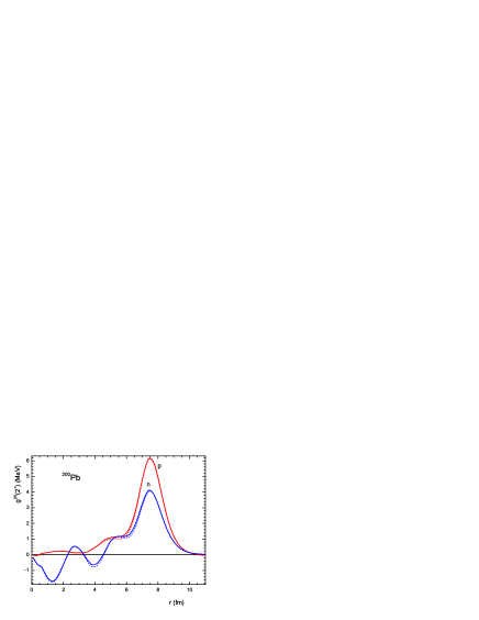
Figure 9: (Color online) The proton and neutron normal transition amplitudes $g^{(0)}$ in ²⁰⁰Pb nucleus. Solid lines correspond to surface pairing, dotted ones, to volume pairing.

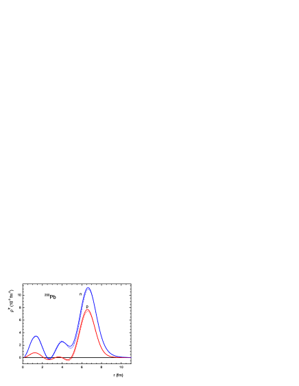
Figure 10: (Color online) The proton and neutron transition densities $\rho^{tr(0)}$ in ²⁰⁰Pb nucleus. Solid lines correspond to surface pairing, dotted ones, to volume pairing.

Let us go to the tin chain. Figs. 11–13 present for the ¹¹⁸Sn nucleus the same quantities which were displayed in Figs. 8–10 for the ²⁰⁰Pb nucleus. This nucleus is in the middle of the chain, and all properties of the “developed” pairing, in particular, particle-hole symmetry should take place. Indeed, now (see Fig. 11) the amplitudes $g^{(1)}$ and $g^{(2)}$ possess a similar form and absolute value and, being of the opposite sign. In the result, we have $|g^{(-)}=g^{(1)}-g^{(2)}|\gg|g^{(+)}=g^{(1)}+g^{(2)}|$ as it should be AB . Again, as in the ²⁰⁰Pb case, the effect of the kind of pairing on the magnitude of $g^{(1,2)}$ is drastic. As to that for the normal amplitudes $g^{(0)}$ and transition densities $\rho^{tr(0)}$, again it is rather moderate but of the another sign. Now in the volume case, the surface peaks in both these quantities are higher and, correspondingly, the $B(E2)$ value is bigger. Evidently, in this case we deal with some destructive interference between normal and anomalous contributions to solutions of the equations of Section 2.

To summarize, we see an effect of the type of pairing on the characteristics of the $2^{+}_{1}$-states in spherical nuclei. The excitation energies $\omega_{2}$ are systematically lower in the surface case to $\delta\omega_{2}\simeq 300\;$keV, and the surface values are, as a rule, closer to the data. For $B(E2)$ values, the effect is not so regular and here the volume version predictions on average look better. Thus, the present analysis is compatible with both volume and surface pairing.

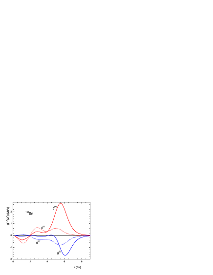
Figure 11: (Color online) The neutron anomalous transition amplitudes $g^{(1,2)}$ in ¹¹⁸Sn nucleus. Solid lines correspond to surface pairing, dotted ones, to volume pairing.

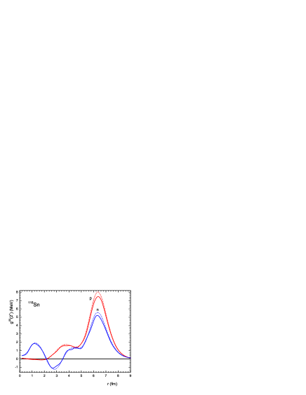
Figure 12: (Color online) The same as in Fig. 9 but for the ¹¹⁸Sn nucleus.

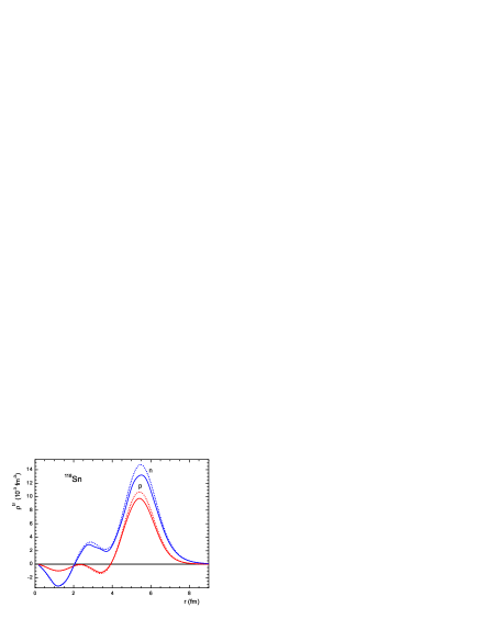
Figure 13: (Color online) The same as in Fig. 10 but for the ¹¹⁸Sn nucleus.

The issue could be naturally raised to what extent the small differences seen in the observables can be traced to the kind of pairing employed. In other words, is it possible to fine tune the interaction parameters such that the both volume and surface pairing produce indistiguishable results, while keeping the mass differences and separation energies close to the experimental data? We carried out such an analysis for the tin chain. We consider the double mass differences

$$D(N)=\frac{1}{2}\left(S_{n}(N)-\frac{1}{2}\left(S_{n}(N-1)+S_{n}(N+1)\right)\right),$$ (30)

$N$ even, which is very sensitive to the value of pairing gap. Note that the approximate relation $D(N)\simeq\bar{\Delta}$ takes place where $\bar{\Delta}$ is an average gap value. We calculate the average difference between theoretical and experimental values of this quantity,

$$\langle\delta D\rangle=\sqrt{\frac{1}{N}\sum_{N}\left(D_{\rm th}(N)-D_{\rm exp}(N)\right)^{2}},$$ (31)

$N$ even. We include into the analysis isotopes from ¹⁰⁶Sn till ¹²⁸Sn for which the developed pairing approximation seems to be reasonable. Results are presented in Table II, for the surface pairing and for three versions of the volume pairing with different values of the strength parameter $f^{\xi}$. For all of them the characteristics of the $2^{+}_{1}$-state in the example ¹¹⁸Sn nucleus are given. It is seen that with increase of $|f^{\xi}|$ from the optimal value $f^{\xi}=-0.33$ deviations from the surface version predictions grow. With decrease of $|f^{\xi}|$ they become less, but this effect is much less than the initial difference even for the value $f^{\xi}=-0.32$ for which description of the mass differences is essentially worse than for the optimal value. An additional decrease of $|f^{\xi}|$ will absolutely destroy the nuclear mass description. In other isotopes of the tin chain, influence of variation of the $f^{\xi}$ parameter to values of $\omega_{2}$ and $B(E2)$ is quite similar. Thus, the effect under discussion originates mainly due to the surface nature of pairing versus the volume one.

Table 2: Dependence of the $2^{+}_{1}$-state characteristics of the ¹¹⁸Sn nucleus on the strength of pairing force.

version	$\langle\delta D\rangle$ (MeV)	$\omega_{2}$ (MeV)	$B(E2,{\rm up)}$(${\rm e^{2}b^{2}}$)
surface	0.10	1.216	0.172
vol. $f^{\xi}=-0.33$	0.11	1.470	0.206
vol. $f^{\xi}=-0.32$	0.16	1.375	0.193
vol. $f^{\xi}=-0.34$	0.11	1.570	0.216

In conclusion of this Section we compare in Fig. 14 the charge transition density $\rho^{\rm tr}_{\rm ch}(r)$ in the ¹¹⁸Sn nucleus with the experimental transition charge density found with a model independent analysis of the elastic electron scattering in rhotr . The theoretical charge density is obtained from $\rho^{\rm tr}_{p}(r)$ and $\rho^{\rm tr}_{n}(r)$ functions displayed in Fig. 13 with taking into account relativistic corrections Friar . For both versions of pairing the agreement with the data is quite reasonable, and it is a little better in the surface case.

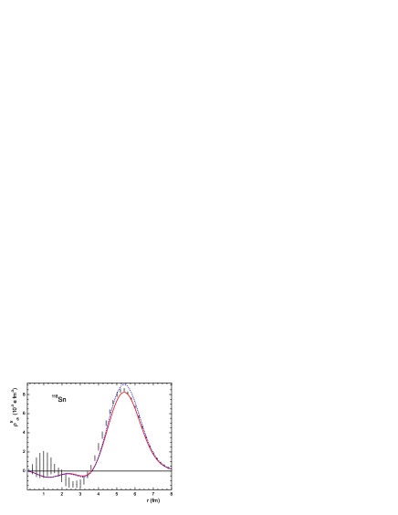
Figure 14: (Color online) The charge transition densities $\rho_{\rm ch}^{{\rm tr}(0)}$ in ¹¹⁸Sn nucleus. Solid lines correspond to surface pairing, dotted ones, to volume pairing.

IV Quadrupole moments of odd nuclei

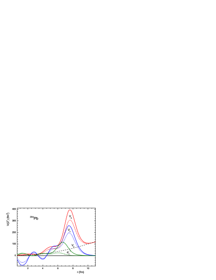
Figure 15: (Color online) Static effective fields $V_{n}$ $V_{p}$ and $d^{+}_{n}$ in ²⁰⁴Pb nucleus. Solid lines correspond to surface pairing, dotted ones, to volume pairing.

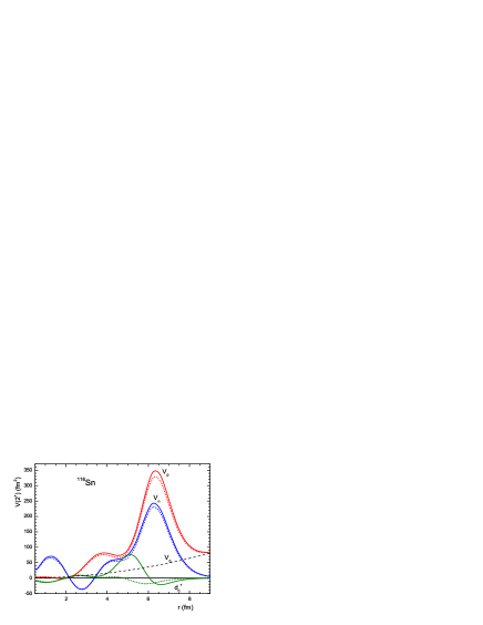
Figure 16: (Color online) Static effective fields $V_{n}$ $V_{p}$ and $d^{+}_{n}$ in ¹¹⁶Sn nucleus. Solid lines correspond to surface pairing, dotted ones, to volume pairing.

Recently magnetic moments of odd spherical nuclei have been calculated borzov2008 ; borzov2010 within the same self-consistent approach as the one used here. A reasonable description of the data for more than hundred of spherical nuclei was obtained. Especially high accuracy was reached for semi-magic nuclei considered in the “single-quasiparticle approximation” where one quasiparticle in the fixed state $\lambda=(n,l,j,m)$ with the energy $\varepsilon_{\lambda}$ is added to the even-even core. According to the TFFS, a quasiparticle differs from a particle of the single-particle model in two respects. First, it possesses the local charge $e_{q}$ (in our case, we have $e_{q}^{p}$ = 1, $e_{q}^{n}$ = 0), and, second, the core is polarized due to the interaction between the particle and the core nucleons via the LM amplitude. In other words, the quasiparticle possesses the effective charge $e_{\rm eff}$ caused by the polarizability of the core which is found by solving the above TFFS equations. In the many-particle Shell Model BABr , a similar quantity is introduced as a phenomenological parameter which describes polarizability of the core consisting of outside nucleons.

In non-magic nuclei, the term quasiparticle takes a double meaning. In addition to the initial LM concept we consider the Bogolyubov quasiparticles with occupation numbers $n_{\lambda}^{\rm B}{=}(E_{\lambda}-\varepsilon_{\lambda})/2E_{\lambda}$ and energies $E_{\lambda}=\sqrt{(\varepsilon_{\lambda}-\mu)^{2}+\Delta_{\lambda}^{2}}$ and solve the set of the QRPA equations (14) instead of one RPA equation.

The success of the single-quasiparticle approximation in describing the magnetic moments of semi-magic nuclei makes it of interest to try to use the same approach for quadrupole moments. In this article, we do such analysis limiting ourselves with odd neighbors of the even tin and lead isotopes considered in the previous Section. To our knowledge, there is no systematic calculations of quadrupole moments of these nuclei.

The static quadrupole moment of an odd nucleus in the single particle state $\lambda$ can be found in terms of the effective field (14) with the static external field $V_{0}=\sqrt{16\pi/5}r^{2}Y_{20}(\theta)$ as follows AB ; solov :

$$Q^{p,n}_{\lambda}=(u^{2}_{\lambda}-v^{2}_{\lambda})V^{p,n}_{\lambda},$$ (32)

where $u_{\lambda}$, $v_{\lambda}$ are the Bogolyubov coefficients and

$$V_{\lambda}=-\frac{2j-1}{2j+2}\int V(r)R_{nlj}^{2}(r)r^{2}dr.$$ (33)

The $j$-dependent factor in (33) appears due to the angular integral BM1 . For $j>1/2$ it is always negative. For odd neighbors of a magic nucleus the “Bogolyubov” factor in (32) reduces to 1 for a particle state and to $-1$ for a hole one.

Components of the static effective field ${\hat{V}}(\omega{=}0)$, that is $V^{n,p}(r)$ and $d_{n}^{+}(r){=}d_{n}^{(1)}(r)+d_{n}^{(2)}(r)$, are displayed in Figs. 15, 16 for ²⁰⁴Pb and ¹¹⁶Sn nuclei, correspondingly. Note that the identity $d^{-}(\omega{=}0){=}0$ takes place AB . One can see large surface maxima of the quantities $V^{n,p}(r)$ similar to those in Figs. 9, 12 for the BM-like transition amplitudes $g^{(0)}_{n,p}(r)$. In-volume (“quantum”) corrections are relatively small, therefore the integral in Eq. (33) is always positive. For protons, it is noticeably larger than the similar integral with the bare field $V^{0}$, see the discussion on the effective charges below.

Diagonal matrix elements (33) of the proton effective field are displayed in Fig. 17 for the tin isotopes and in Fig. 18, for the lead ones. As it is seen, for a major part of the tin isotopes, the difference between values of proton matrix elements $V^{p}_{\lambda}$ surface and volume pairing is quite small. Only for ^112-116Sn nuclei it reaches 10%. In the lead region, the difference is more pronounced reaching $\simeq 30\div 40$% for $9/2^{-}$ and $11/2^{-}$ states.

Corresponding quadrupole moments for nuclei with odd proton number $Z=50\pm 1$ and $Z=82\pm 1$ are presented in Table III. As it was noted above, in this case the Bogolyubov factor in (32) is trivial, equal to $\pm 1$. In order to check our approach, we selected only nuclei where there are experimental data and those which satisfy presumably the single-quasiparticle approximation. In particular, we excluded several light Tl isotopes with known quadrupole moments of low-lying excited $9/2^{-}$ states. If to suppose that they are single-quasiparticle $1h_{9/2}$ states, they should have essentially higher excitation energies than it takes place.

Table 3: Quadrupole moments $Q\;$(e b) of odd-proton nuclei.

nucl.	$\lambda_{0}$	$Q_{\rm exp}$	$Q_{\rm th}^{\rm surf}$	$Q_{\rm th}^{\rm vol}$	$Q_{0}$	$e_{\rm eff}^{\rm surf}$	$e_{\rm eff}^{\rm vol}$
105In	$1g_{9/2}$	+0.83(5)	+0.83	+0.90	+0.18	4.6	5.0
107In	$1g_{9/2}$	+0.81(5)	+0.98	+1.07	+0.18	5.4	5.9
109In	$1g_{9/2}$	+0.84(3)	+1.11	+1.14	+0.18	6.2	6.3
111In	$1g_{9/2}$	+0.80(2)	+1.16	+1.10	+0.19	6.1	5.8
113In	$1g_{9/2}$	+0.80(4)	+1.12	+1.02	+0.19	5.9	5.4
115In	$1g_{9/2}$	+0.81(5), 0.58(9)	+1.03	+0.97	+0.19	5.4	5.1
117In	$1g_{9/2}$	+0.829(10)	+0.96	+0.95	+0.19	5.1	5.0
119In	$1g_{9/2}$	+0.854(7)	+0.91	+0.92	+0.19	4.8	4.8
121In	$1g_{9/2}$	+0.814(11)	+0.83	+0.84	+0.19	4.4	4.4
123In	$1g_{9/2}$	+0.757(9)	+0.74	+0.74	+0.19	3.9	3.9
125In	$1g_{9/2}$	+0.71(4)	+0.66	+0.74	+0.19	3.8	3.9
127In	$1g_{9/2}$	+0.59(3)	+0.55	+0.49	+0.19	2.9	2.6
115Sb	$2d_{5/2}$	-0.36(6)	-0.88	-0.81	-0.14	6.3	5.8
117Sb	$2d_{5/2}$	-0(2)	-0.82	-0.77	-0.14	5.9	5.5
119Sb	$2d_{5/2}$	-0.37(6)	-0.77	-0.76	-0.14	5.5	5.4
121Sb	$2d_{5/2}$	-0.36(4), -0.45(3)	-0.72	-0.73	-0.14	5.1	5.2
	$1g_{7/2}^{\,*}$	-0.48(5)	-0.81	-0.81	-0.17	4.8	4.8
123Sb	$1g_{7/2}$	-0.49(5)	-0.74	-0.74	-0.17	4.4	4.4
205Tl	$3d_{3/2}^{\,*}$	0.74(15)	+0.23	+0.23	+0.12	1.9	1.9
203Bi	$1h_{9/2}$	-0.68(6)	-1.32	-0.91	-0.25	5.3	3.6
205Bi	$1h_{9/2}$	-0.59(4)	-0.94	-0.72	-0.25	3.8	2.9
209Bi	$1h_{9/2}$	-0.37(3), -0.55(1)	-0.34	-0.34	-0.25	1.4	1.4
		-0.77(1), -0.40(5)

Table 4: Quadrupole moments $Q\;$(e b) of odd-neutron nuclei.

nucleus	$\lambda_{0}$	$Q_{\rm exp}$	$Q_{\rm th}^{\rm surf}$	$Q_{\rm th}^{\rm vol}$	$e_{\rm eff}^{\rm surf}$	$e_{\rm eff}^{\rm vol}$
109Sn	$2d_{5/2}$	+0.31(10)	+0.25	+0.27	3.5	3.7
111Sn	$1g_{7/2}$	+0.18(9)	+0.05	+0.10	4.0	3.9
113Sn	$1h_{11/2}^{\,*}$	0.41(4), 0.48(5)	-0.78	-0.75	4.4	4.1
115Sn	$1g_{7/2}^{\,*}$	0.26(3)	+0.38	+0.38	3.9	3.6
	$1h_{11/2}^{\,*}$	0.38(6)	-0.70	-0.67	4.2	3.8
117Sn	$1h_{11/2}^{\,*}$	-0.42(5)	-0.59	-0.58	3.9	3.7
119Sn	$2d_{3/2}^{\,*}$	+0.094(11),	-0.03	-0.02	3.0	2.9
		-0.065(5),
		-0.061(3)
	$1h_{11/2}^{\,*}$	0.21(2)	-0.46	-0.45	3.6	3.5
121Sn	$2d_{3/2}$	-0.02(2)	+0.06	+0.08	2.9	2.9
	$1h_{11/2}^{\,*}$	-0.14(3)	-0.29	-0.29	3.3	3.3
123Sn	$1h_{11/2}$	+0.03(4)	-0.12	-0.10	3.0	2.9
125Sn	$1h_{11/2}$	+0.1(2)	+0.04	+0.06	2.7	2.7
191Pb	$1i_{13/2}^{\,*}$	+0.085(5)	+0.0004	+0.10	5.3	5.9
193Pb	$1i_{13/2}^{\,*}$	+0.195(10)	+0.33	+0.39	6.5	5.5
195Pb	$1i_{13/2}^{\,*}$	+0.306(15)	+0.69	+0.66	6.6	5.2
197Pb	$3p_{3/2}$	-0.08(17)	+0.19	+0.14	5.2	3.8
	$1i_{13/2}^{\,*}$	+0.38(2)	+0.98	+0.78	6.4	4.6
199Pb	$3p_{3/2}$	+0.08(9)	+0.27	+0.19	4.5	3.1
201Pb	$2f_{5/2}$	-0.01(4)	+0.14	+0.09	4.2	2.8
203Pb	$2f_{5/2}$	+0.10(5)	+0.28	+0.22	3.2	2.3
205Pb	$2f_{5/2}$	+0.23(4)	+0.34	+0.28	2.6	2.0
	$1i_{13/2}^{\,*}$	0.30(5)	+0.67	+0.56	3.0	2.2
209Pb	$2g_{9/2}$	-0.3(2)	-0.26	-0.26	0.9	0.9

Experimental data are taken from the compilation Q-data . From several cases of proton excited isomeric states we limit ourselves with only two, the $1g_{7/2}^{\,*}$ state in the ¹²¹Sb and $2d_{3/2}^{\,*}$ state in ²⁰⁵Tl nuclei, for which the hypothesis on the single-quasiparticle structure seems to us more or less safe. Again, we presented results for both the kinds of nuclear pairing (the quantities $Q_{\rm th}^{\rm surf}$ and $Q_{\rm th}^{\rm vol}$ for surface and volume pairing, correspondingly). In the 6-th column of the table, the single-particle quadrupole moment is presented which is found from Eqs. (32), (33) with substitution $V\to V_{0}$. As it follows from Fig. 17, for odd-proton neighbors of the tin isotopes, difference between values of quadrupole moments for surface and volume pairing is quite small, in limits of 10%. In the lead region, see Fig. 18, the difference is more pronounced, but here the number of the data is very small, only 4. In addition, only in the ^203,205Bi and ²⁰⁵Tl case neutron pairing exists. For these nuclei, the effect under discussion reaches $\simeq 30\div 40$%.

For the long chain of twelve In isotopes agreement with the data is quite reasonable. For five Sb isotopes (six values of the quadrupole moment) agreement is rather poor, disagreement reaching $\simeq 50\div 100$%. A similar situation takes place for two lighter Bi isotopes. For the ²⁰⁹Bi isotope where pairing is absent experimental data are contradictory. We think that the main reason of existing disagreements is neglecting the phonon coupling effects.

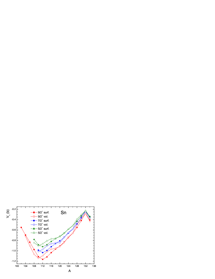
Figure 17: (Color online) Diagonal matrix elements $V^{p}_{\lambda}$ of the effective proton quadrupole field in the tin isotopes. Solid lines correspond to surface pairing, dotted ones, to volume pairing.

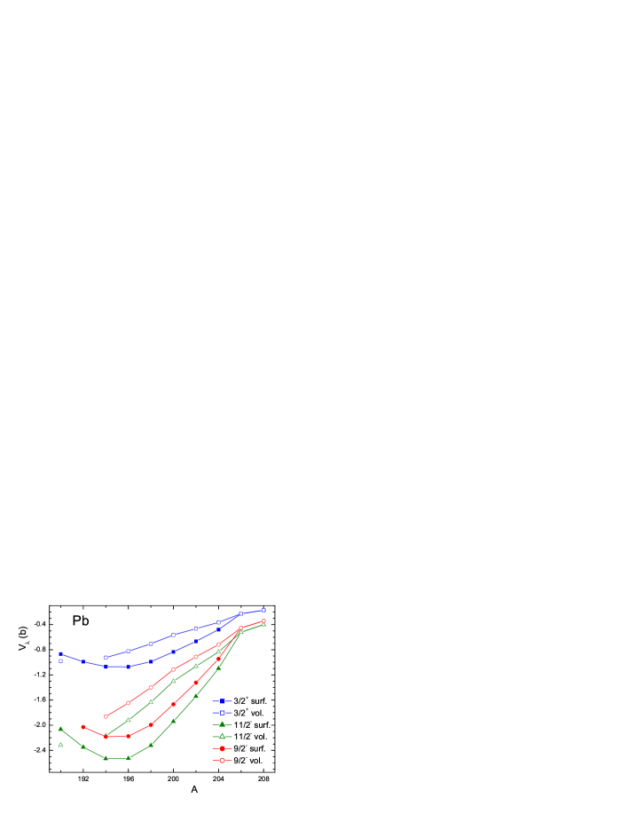
Figure 18: (Color online) The same as in Fig. 17, but for the lead isotopes.

Let us go to odd-neutron nuclei, the odd tin and lead isotopes. The results are presented in Table IV and Figs. 19,20. In selecting nuclei for the table, we used the same concept as for protons. In this case, we included into the analysis twelve excited states, in addition to the ground ones. With the only exception of the ²⁰⁹Pb nucleus, all the nuclei under consideration exhibit pairing effects and the factor $(u^{2}_{\lambda}-v^{2}_{\lambda})$ in Eq. (32) becomes non-trivial. It changes permanently depending on the state $\lambda$ and the nucleus under consideration. Note that in the case of magnetic moments the factor of $(u^{2}_{\lambda}+v^{2}_{\lambda})=1$ appears in the relation analogous to (32) solov . In our case, this factor determines the sign of the quadrupole moment. In all cases when the sign of the experimental moment is known the theoretical sign is correct. This permits to use our predictions to determine the sign when it is unknown. The factor under discussion depends essentially on values of the single-particle basis energies $\varepsilon_{\lambda}$ reckoned from the chemical potential $\mu$ as we have $(u^{2}_{\lambda}-v^{2}_{\lambda})=(\varepsilon_{\lambda}-\mu)/E_{\lambda}$. Keeping in mind such sensitivity, we found this quantity for a given odd nucleus $(Z,N+1)$, $N$ even, with taking into account the blocking effect in the pairing problem solov putting the odd neutron to the state $\lambda$ under consideration. For the $V_{\lambda}$ value in Eq. (32) we used the half-sum of these values in two neighboring even nuclei. We consider agreement with the data reasonable if we have $|Q_{\rm th}-Q_{\rm exp}|<0.1\div 0.2\;$e b. If to use such a criterion, there are 7 “bad” cases in Table IV, and 16 “good”. Several rather strong disagreements with the experimental data in Table IV for high-j levels $1h_{11/2}$ in Sn isotopes and $1i_{13/2}$ in Pb isotopes originate just from their too distant positions from the Fermi level. Thus, the $Q$ values depend strongly on the single-particle level structure. Again, as for protons, the difference between predictions of the two models under consideration is, as a rule, rather small, and only for $1i_{13/2}$-states in the lead chain it reaches $\simeq 20\div 30$%.

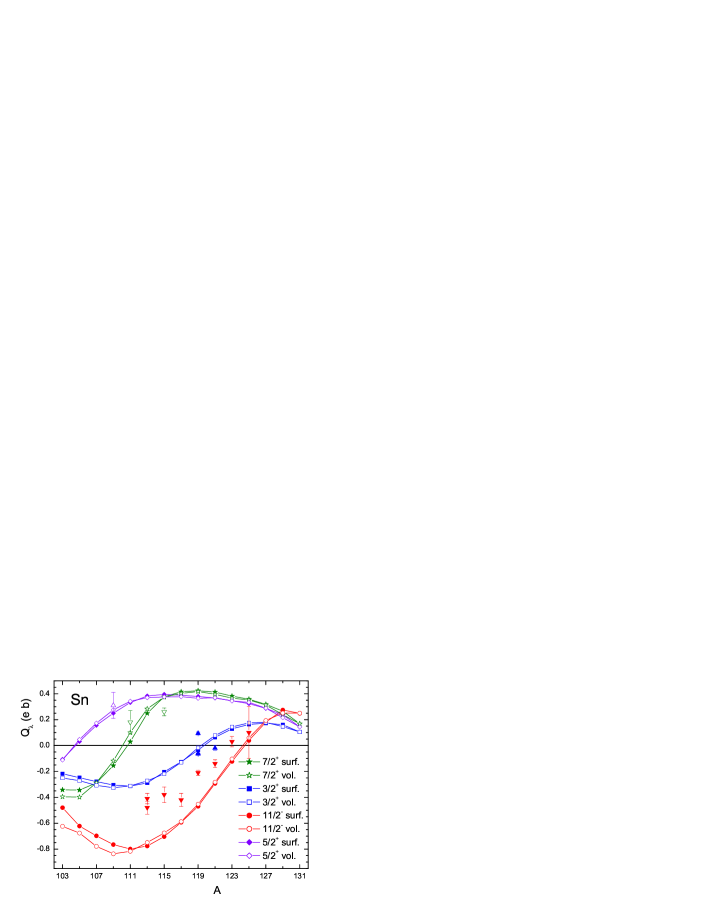
Figure 19: (Color online) Quadrupole moments of odd tin isotopes. Solid lines correspond to surface pairing, dotted ones, to volume pairing. Experimental data are shown with $\blacktriangle$ for $3/2^{+}$, $\blacktriangledown$ for $11/2^{-}$, $\vartriangle$ for $5/2^{+}$, and $\triangledown$ for $7/2^{+}$ states.

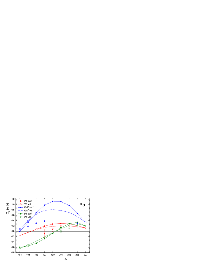
Figure 20: (Color online) Quadrupole moments of odd lead isotopes. Solid lines correspond to surface pairing, dotted ones, to volume pairing. Experimental data are shown with $\blacktriangle$ for $13/2^{+}$, $\blacktriangledown$ for $3/2^{-}$, and $\vartriangle$ for $5/2^{-}$ states.

In the last two columns of Tables III and IV, the effective charges are presented which are defined as $e_{\rm eff}^{p,n}=V^{p,n}_{\lambda}/(V_{0}^{p})_{\lambda}$. It is a direct characteristic of the core polarizability by the quadrupole external field. In these tables, there are only two nuclei, ²⁰⁹Bi and ²⁰⁹Pb, with a double-magic core, and in this case the polarizability is rather moderate, $e^{p}_{\rm eff}=1.4,e^{n}_{\rm eff}=0.9$. In nuclei with an unfilled neutron shell it becomes much stronger, $e_{\rm eff}\simeq 3\div 6$. The reason is rather obvious. Indeed, for the case of a positive parity field $V_{0}$, virtual transitions inside the unfilled shell begin to contribute and small energy denominators appear in the propagator ${\cal L}^{n}$ (18) playing the main role in the problem under consideration. It enhances the neutron response to the field $V_{0}$ and, via the strong LM neutron-proton interaction amplitude ${\cal F}^{np}$, the proton response as well. Results for the chain ^203,205,209Bi show how the polarizability grows with increase of the number of neutron holes. Keeping in mind this physics, one can represent the effective charges as $e^{p}_{\rm eff}=1+e^{p}_{\rm pol},e^{n}_{\rm eff}=e^{n}_{\rm pol}$ where $e^{p,n}_{\rm pol}$ is the pure polarizability charge. To separate contributions of the unfilled shells and core nucleons explicitly, one can divide the Hilbert space of the QRPA equations (14) to the “valent” and subsidiary ones and carry out the corresponding renormalization procedure kaevst .

V Discussion and conclusions

The effect of the density dependence of the pairing interaction to low-lying quadrupole excitations in spherical nuclei is analyzed for two isotopic chains of semi-magic nuclei. Static quadrupole moments of neighboring odd nuclei are also examined. The complete set of the QRPA-like TFFS equations for response functions is solved in a self-consistent way within the EDF approach to superfluid nuclei with previously fixed parameters of the functional. The DF3-a functional Tol-Sap is used which is a small modification of the functional DF3 Fay ; Fay5 . Specifically, spin-orbit and effective tensor terms of the initial EDF DF3 were changed. Two models for effective pairing force are considered, the surface and the volume ones, which give rise to approximately the same accuracy in reproducing mass differences. A noticeable effect in excitation energies $\omega_{2}$ is found: predictions for the volume model are systematically higher than the surface ones by $\delta\omega_{2}\simeq 200\div 300\;$keV. As to the excitation probabilities $B(E2,{\rm up})$, the effect is not so regular, however, as a rule, the volume values are also higher. Thus, the correlation between these two quantities typical for the BM model, where a higher frequency always results in a lower probability, is destroyed. On the average, both models reasonably agree with the data. In addition, they both reproduce rather well the model-independent charge density $\rho^{\rm tr}_{\rm ch}(2^{+}_{1})$ for the ¹¹⁸Sn nucleus.

Comparison with recent QRPA calculations Bertsch1 with the Skyrme force SkM* and SLy4 shows that for the lead chain they agree with the data a little better than our results but for the tin chain the situation is opposite and our predictions occur to be essentially better. The surface model is systematically better in describing the energies $\omega_{2}$ whereas the excitation probabilities are, as a rule, reproduced better with the volume model.

Whereas the charge radii study Fay and ab initio theory of paring Bald1 ; milan3 favor the surface pairing, the $\omega(2^{+}_{1})$ and $B(E2,{\rm up})$ data do not allow to prefer any of the two kinds of pairing.

A reasonable agreement with experiment for the quadrupole moments of odd neighbors of the even tin and lead isotopes has been obtained for the most part of nuclei considered. For odd-proton this confirms that the single-quasiparticle approximation works sufficiently well. For odd-neutron isotopes under consideration, validity of this approach was checked previously with the analysis of magnetic moments borzov2010 . In the case we consider, the problem is more complicated than for odd proton isotopes as the Bogolyubov factor $(u^{2}_{\lambda}-v^{2}_{\lambda})=(\varepsilon_{\lambda}-\mu)/E_{\lambda}$ comes to the quadrupole moment value, in addition to the matrix element of the effective field $V_{\lambda}$. This factor makes the quadrupole moment value very sensitive to accuracy of calculating the single-particle energy $\varepsilon_{\lambda}$ of the state under consideration, especially near the Fermi surface as the quantity $Q_{\lambda}$ vanishes at $\varepsilon_{\lambda}=\mu$. For such a situation, the influence of the coupling of single-particle degrees of freedom with phonons, see borzov2010 ; kaev2011 , should be especially important. This rather complicated problem will be considered separately.

As to the effect of the density dependence of pairing, for quadrupole moments it is, on the average, less than for quadrupole transitions. It depends on a nucleus examined and on the odd-nucleon state as well. In the tin region, it is, as a rule, of the order of $\simeq 10$%. However, in the lead region it is higher and reaches $\simeq 30\div 50$% for ^203,205Bi and ²⁰⁵Pb.

VI Acknowledgment

We thank J. Engel and J. Terasaki for kind supplying us with tables of the results of the QRPA calculations Bertsch1 with the SkM* and SLy4 force. Four of us, S. T., S. Ka., E. S., and D. V., are grateful to Institut für Kernphysik, Forschungszentrum Jülich for hospitality. The work was partly supported by the DFG and RFBR Grants Nos.436RUS113/994/0-1 and 09-02-91352NNIO-a, by the Grants NSh-7235.2010.2 and 2.1.1/4540 of the Russian Ministry for Science and Education, and by the RFBR grants 09-02-01284-a, 11-02-00467-a.

References

- (1) T. Niksic, D. Vretenar, and P. Ring, Prog. Part. Nucl. Phys. 66, 519 (2011).
- (2) J. Erler et al. Phys. Part. Nucl. 41, 851 (2010).
- (3) M. Bender, P.-H. Heenen, and P.-G. Reinhard, Rev. Mod. 75, 121 (2003).
- (4) W. Kohn and L. J. Sham, Phys. Rev. 140, A 1133 (1965).
- (5) R. O. Jones, O. Gunnarson, Rev. Mod. Phys. 61, 689 (1989).
- (6) L. N. Oliveira, E. K. U. Gross, and W. Kohn, Phys. Rev. Lett. 60, 2430 (1988).
- (7) D. N. Basov et al., Rev. Mod. Phys. 83, 473 (2011).
- (8) V. A. Khodel and E. E. Saperstein, Phys. Rep. 92, 183 (1982).
- (9) A. B. Migdal, Theory of finite Fermi systems and applications to atomic nuclei (Wiley, New York, 1967).
- (10) S. A. Fayans and V. A. Khodel, JETP Lett. 17, 633 (1973).
- (11) V. A. Khodel, E. E. Saperstein, and M. V. Zverev, Nucl. Phys. A465, 397 (1987).
- (12) A. V. Smirnov, S. V. Tolokonnikov, and S. A. Fayans, Sov. J. Nucl. Phys. 48, 995 (1988).
- (13) S. A. Fayans, JETP Letters 68, 169 (1998).
- (14) S. A. Fayans, S. V. Tolokonnikov, E. L. Trykov, and D. Zawischa, Nucl. Phys. A676, 49 (2000).
- (15) J. Erler, P. Klüpfel, and P.-G. Reinhard, Phys. Rev. C 82, 044307 (2010).
- (16) E. Epelbaum, H. -W. Hammer, U. -G. Meissner, Rev. Mod. Phys. 81, 1773-1825 (2009). [arXiv:0811.1338 [nucl-th]].
- (17) J. E. Drut, R. J. Furnstahl, L. Platter, Prog. Part. Nucl. Phys. 64, 120-168 (2010). [arXiv:0906.1463 [nucl-th]].
- (18) M. Baldo, U. Lombardo, E. E. Saperstein, and M. V. Zverev, Phys. Lett. B477, 410 (2000).
- (19) M. Baldo, U. Lombardo, E. E. Saperstein, M. V. Zverev, Phys. Rep. 391 261, (2004).
- (20) M. Baldo, U. Lombardo, S. S. Pankratov, and E. E. Saperstein, J. Phys. G: Nucl. Phys. 37, 064016 (2010).
- (21) S. S. Pankratov, M. V. Zverev, M. Baldo, U. Lombardo, and E. E. Saperstein, [arXiv:1103.4137 [nucl-th], to be published in Phys. Rev. C.
- (22) F. Barranco, R. A. Broglia, H. Esbensen, and E. Vigezzi, Phys. Lett. B390, 13 (1997).
- (23) F. Barranco, R. A. Broglia, G. Colo, et al., Eur. Phys. J. A 21, 57 (2004).
- (24) A. Pastore, F. Barranco, R. A. Broglia, and E. Vigezzi, Phys. Rev. C 78, 024315 (2008).
- (25) Aurel Bulgac and Yongle Yu, Phys. Rev. Lett. 88, 042504 (2002).
- (26) Yongle Yu and Aurel Bulgac, Phys. Rev. Lett. 90, 222501 (2003).
- (27) J. Terasaki, J. Engel, and G. F. Bertsch, Phys. Rev. C 78, 044311 (2008).
- (28) A. P. Severyukhin, V. V. Voronov, and Nguyen Van Giai, Phys. Rev. C 77, 024322 (2008).
- (29) G. F. Bertsch, M. Girod, S. Hilaire, J.-P. Delaroche, H. Goutte, and S. Péru, Phys. Rev. Lett. 99, 032502 (2007).
- (30) S. V. Tolokonnikov and E. E. Saperstein, Phys. Atom. Nucl. 73, 1684 (2010).
- (31) D. J. Horen, G. R. Satchler, S. A. Fayans, and E. L. Trykov, Nucl. Phys. A600, 193 (1996).
- (32) E. E. Saperstein and S. V. Tolokonnikov, Phys. Atom. Nucl. 73, to be published (2011).
- (33) A. B. Migdal, Theory of finite Fermi systems and applications to atomic nuclei, Second Edition (in Russian, Moscow, “Nauka”, 1982).
- (34) E. E. Saperstein and M. A. Troitsky, Sov. J. Nucl. Phys. 1, 284 (1965).
- (35) M. V. Zverev and E. E. Saperstein, Sov. J. Nucl. Phys. 42, 683 (1985).
- (36) S. Goriely, N. Chamel, and J. M. Pearson, Phys. Rev. Lett. 102, 152503 (2009).
- (37) S. T. Belyaev, A. V. Smirnov, S. V. Tolokonnikov, S. A. Fayans, Sov. J. Nucl. Phys. 48, 995 (1988).
- (38) S. Goriely, http://www-astro.ulb.ac.be/Html/masses. html
- (39) Abhishek Mukherjee, Y. Alhassid, and G. F. Bertsch, Phys. Rev. C 83, 014319 (2011).
- (40) S. Raman, C. W. Nestor Jr., and P. Tikkanen, Atom. Data Nucl. Data Tables 78, 1 (2001).
- (41) A. Bohr and B. R. Mottelson, Nuclear Structure (Benjamin, New York, Amsterdam, 1974.), Vol. 2.
- (42) D. C. Radford, et al., Nucl. Phys. A752, 264c (2005).
- (43) J. Cederkäll, et al., Phys. Rev. Lett. 98, 172501 (2007).
- (44) C. Vaman, et al., Phys. Rev. Lett. 99, 162501 (2007).
- (45) A. Ekström, et al., Phys. Rev. Lett. 101, 012502 (2008).
- (46) J. E. Wise, et al., Phys. Rev. C 45, 2701 (1992).
- (47) J. L. Friar, J. Heisenberg, and J. W. Negele, in Proceedings of the June Workshop in Intermediate Energy Electromagnetic Interactions, Ed. by A.M. Bernstein (Massachusetts Institute of Technology, 1977), p. 325.
- (48) I. N. Borzov, E. E. Saperstein, and S. V. Tolokonnikov, Phys. Atom. Nucl. 71, 469 (2008).
- (49) I. N. Borzov, E. E. Saperstein, S. V. Tolokonnikov, G. Neyens, and N. Severijns, EPJ A 45, 159 (2010).
- (50) M. Honma, T. Otsuka, B. A. Brown, T. Mizusaki, Phys. Rev. C 69, (2004) 034335.
- (51) V. G. Soloviev, Theory of Complex Niclei, (Oxford: Pergamon Press, 1976).
- (52) A. Bohr and B. R. Mottelson, Nuclear Structure (Benjamin, New York, Amsterdam, 1969.), Vol. 1.
- (53) N. J. Stone, Atom. Data Nucl. Data Tables, 90, 75 (2005).
- (54) S. P. Kamerdzhiev, Sov. Nucl. Phys. 9, 324 (1969).
- (55) S. P. Kamerdzhiev, A. V. Avdeenkov and D. A. Voitenkov, Phys. Atom. Nucl. 73, to be published (2011).