Evaluating Data Assimilation Algorithms
ABSTRACT
Data assimilation leads naturally to a Bayesian formulation in which the posterior probability distribution of the system state, given all the observations on a time window of interest, plays a central conceptual role. The aim of this paper is to use this Bayesian posterior probability distribution as a gold standard against which to evaluate various commonly used data assimilation algorithms.
A key aspect of geophysical data assimilation is the high dimensionality and limited predictability of the computational model. We study the 2D Navier-Stokes equations in a periodic geometry, which has these features and yet is tractable for explicit and accurate computation of the posterior distribution by state-of-the-art statistical sampling techniques. The commonly used algorithms that we evaluate, as quantified by the relative error in reproducing moments of the posterior, are 4DVAR and a variety of sequential filtering approximations based on 3DVAR and on extended and ensemble Kalman filters.
The primary conclusions are that under the assumption of a well-defined posterior probability distribution: (i) with appropriate parameter choices, approximate filters can perform well in reproducing the mean of the desired probability distribution; (ii) however they do not perform as well in reproducing the covariance; (iii) the error is compounded by the need to modify the covariance, in order to induce stability. Thus, filters can be a useful tool in predicting mean behavior, but should be viewed with caution as predictors of uncertainty. These conclusions are intrinsic to the algorithms when assumptions underlying them are not valid and will not change if the model complexity is increased.
1 Introduction
The positive impact of data assimilation schemes on numerical weather prediction (NWP) is unquestionable. Improvements in forecast skill over decades reflect not only the increased resolution of the computational model, but also the increasing volumes of data available, and the increasing sophistication of algorithms to incorporate this data. However, because of the huge scale of the computational model, many of the algorithms used for data assimilation employ approximations, based on both physical insight and computational expediency, whose effect can be hard to evaluate. The aim of this paper is to describe a method of evaluating some important aspects of data assimilation algorithms, by comparing them with a gold-standard: the Bayesian posterior probability distribution on the system state given observations. In so doing we will demonstrate that carefully chosen filters can perform well in predicting mean behaviour, but that they typically perform poorly when predicting uncertainty, such as covariance information.
In typical operational conditions the observed data, model initial conditions, and model equations are all subject to uncertainty. Thus we take the perspective that the gold standard, which we wish to reproduce as accurately as possible, is the (Bayesian) posterior probability distribution of the system state (possibly including parameters) given the observations. For practical weather forecasting scenarios this is not computable. The two primary competing methodologies for data assimilation that are computable, and hence are implemented in practice, are filters Kalnay (2003) and variational methods Bennett (2002). We will compare the (accurately computed, extremely expensive) Bayesian posterior distribution with the output of the (approximate, relatively cheap) filters and variational methods used in practice. Our underlying dynamical model is the 2D Navier-Stokes equations in a periodic setting. This provides a high dimensional dynamical system, which exhibits a range of complex behaviours, yet which is sufficiently small that the Bayesian posterior may be accurately computed by state-of-the-art statistical sampling in an off-line setting.
The idea behind filtering is to update the posterior distribution of the system state sequentially at each observation time. This may be performed exactly for linear systems subject to Gaussian noise, and is then known as the Kalman filter Kalman (1960); Harvey (1991). For nonlinear or non-Gaussian scenarios the particle filter Doucet et al. (2001) may be used and provably approximates the desired probability distribution as the number of particles is increased Bain and Crişan (2008). However in practice this method performs poorly in high dimensional systems Snyder et al. (2008) and, whilst there is considerable research activity aimed at overcoming this degenertation van Leeuwen (2010); Chorin et al. (2010); Bengtsson et al. (2003), it cannot currently be viewed as a practical tool within the context of geophysical data assimilation. In order to circumvent problems associated with the representation of high dimensional probability distributions some form of Gaussian approximation is typically used to create practical filters. The oldest and simplest such option is to use a nonlinear generalization of the mean update in the Kalman filter, employing a constant prior covariance operator, obtained offline through knowledge coming from the underlying model and past observations Lorenc (1986); this methodology is sometimes refered to as 3DVAR. More sophisticated approximate Gaussian filters arise from either linearizing the dynamical model, yielding the extended Kalman filter Jazwinski (1970), or utilizing ensemble statistics, leading to the ensemble Kalman filter Evensen et al. (1994); Evensen (2003). Information about the underlying local (in time) Lyapunov vectors, or bred vectors (see Kalnay (2003) for discussion) can be used to guide further approximations that are made when implementing these methods in high dimensions. We will also be interested in the use of Fourier diagonal filters, introduced in Harlim and Majda (2008); Majda et al. (2010), which approximate the dynamical model by a statistically equivalent linear dynamical system in a manner which enables the covariance operator to be mapped forward in closed form; in steady state the version we employ here reduces to a particular choice of 3DVAR, based on climatological statistics. An overview of particle filtering for geophysical systems may be found in Van Leeuwen (2009) and a quick introduction to sequential filtering may be found in Arulampalam et al. (2002).
Whilst filtering updates the system state sequentially each time when a new observation becomes available variational methods attempt to incorporate data which is distributed over an entire time-interval. This may be viewed as an optimization problem where the objective function is to choose the initial state, and possibly forcing to the physical model, in order to best match the data over the specified time-window. As such it may be viewed as a PDE-constrained optimization problem Hinze et al. (2008), and more generally as a particular class of regularized inverse problem Vogel (2002); Tarantola (2005); Banks and Kunisch (1989). This approach is referred to as 4DVAR in the geophysical literature, when the optimization is performed over just the initial state of the system Talagrand and Courtier (1987); Courtier and Talagrand (1987) and as weak constraint 4DVAR when optimization is also over forcing to the system Zupanski (1997).
From a Bayesian perspective, the solution to an inverse problem is statistical, rather than deterministic, and is hence significantly more challenging: regularization is imposed through viewing the unknown as a random variable, and the aim is to find the posterior probability distribution on the state of the system on a given time window, given the observations on that time window. With the current and growing capacity of computers it is becoming relevant and tractable to begin to explore such approaches to inverse problems in differential equations Kaipio and Somersalo (2005), even though it is currently infeasible to do so for NWP. There has, however, been some limited study of the Bayesian approach to inverse problems in fluid mechanics using path integral formulations in continuous time as introduced in Apte et al. (2007); see Apte et al. (2008a, b); Quinn and Abarbanel (2010); Cotter et al. (2011) for further developments. We will build on the algorithmic experience contained in these papers here. For a recent overview of Bayesian methodology for inverse problems in differential equations, see Stuart (2010), and for the Bayesian formulation of a variety of inverse problems arising in fluid mechanics see Cotter et al. (2009). The key take home message of this body of work on Bayesian inverse problems is that it is often possible to compute the posterior distribution of state given noisy data with high degree of accuracy, albeit at great expense: the methodology could not be used online as a practical algorithm, but provides us with a gold-standard against which we can evaluate on-line approximate methods used in practice.
There are several useful connections to make between the Bayesian posterior distribution, filtering methods and variational methods all of which serve to highlight the fact that they are all attempting to represent related quantities. The first observation is that, in the linear Gaussian setting, if backward filtering is implemented on a given time window (this is known as smoothing) after forward filtering, then the resulting mean is equivalent to 4DVAR Fisher et al. (2005). The second observation is that the Bayesian posterior distribution at the end of the time window, which is a non-Gaussian version of the Kalman smoothing distribution just described, is equal to the exact filtering distribution at that time, provided the filter is initialized with the same distribution as that chosen at the start of the time window for the Bayesian posterior model Stuart (2010). The third observation is that the 4DVAR variational method corresponds to maximizing the Bayesian posterior distribution and is known in this context as a MAP estimator Cox (1964); Kaipio and Somersalo (2005). More generally, connections between filtering and smoothing have been understood for some time Bryson and Frazier (1963).
For the filtering and variational algorithms implemented in practice, these connections may be lost, or weakened, because of the approximations made to create tractable algorithms. Hence we attempt to evaluate these algorithms by their ability to reproduce moments of the Bayesian posterior distribution since this provides an unequivocal notion of a perfect solution, given a complete model description, including sources of error; we hence refer to it as the gold standard. We emphasize that we do not claim to present optimal implementations of any method except the gold standard MCMC. Nonetheless, the phenomena we observe and the conclusions we arrive at will not change qualitatively if the algorithms are optimized. They reflect inherent properties of the approximations used to create online algorithms useable in practical online scenarios.
The ability of filters to track the signal in chaotic systems has been the object of study in data assimilation communities for some time and we point to the paper Miller et al. (1994) as an early example of this work, confined to low dimensional systems, and to the more recent Carrassi et al. (2008) for study of both low and high dimensional problems, and for further discussion of the relevant literature. As mentioned above, we develop our evaluation in the context of the 2D Navier Stokes equations in a periodic box. We work in parameter regimes in which at most Fourier modes are active. This model has several attractive features. For instance, it has a unique global attractor with a tunable parameter, the viscosity (or, equivalently the Reynolds number), which tunes between a one-dimensional stable fixed point and very high-dimensional strongly chaotic attractor Temam (2001). As the dimension of the attractor increases, many scales are present, as one would expect in a model of the atmosphere. By working with dimensions of size we have a model of significantly higher dimension than the typical toy models that one encounters in the literature Lorenz (1996, 1963). Therefore, while the 2D Navier-Stokes equations do not model atmospheric dynamics, we expect the model to exhibit similar predictability issues as arise atmospheric models, and this fact, together their high dimensionaliy, makes them a useful model with which to study aspects of atmospheric data assimilation. However we do recognize the need for follow-up studies which investigate similar issues for models such as Lorenz-96, or quasi-geostrophic models, which can mimic or model the baroclinic instabilities which drive so much of atmospheric dynamics.
The primary conclusions of our study are that: (i) with appropriate parameter choices, approximate filters can perform well in reproducing the mean of the desired probability distribution; (ii) however these filters typically perform poorly when attempting to reproduce information about covariance as the assumptions underlying them may not be valid (iii) this poor performance is compounded by the need to modify the filters, and their covariance in particular, in order to induce filter stability and avoid divergence. Thus, whilst filters can be a useful tool in predicting mean behaviour, they should be viewed with caution as predictors of uncertainty. These conclusions are intrinsic to the algorithms and will not change if the model is more complex, for example resulting from a smaller viscosity in our model. We reiterate that these conclusions are based on our assumption of well-defined initial prior, observational error, and hence Bayesian posterior distributions. Due to the computational cost of computing the latter we look only at one, initial, interval of observations, but upon our assumption, the accuracy over this first interval will limit accuracy on all subsequent intervals, and they will not become better. Under the reasonable assumption that the process has finite correlation time, the initial prior will be forgotten eventually and, in the present context, this effect would be explored by choosing different priors coming from approximation of the asymptotic distribution by some filtering algorithm and/or climatological statistics and testing the robustness of conclusions, and indeed of the filtering distribution itself, to changes in prior. The question of sensitivity of the results to choice of prior is not addressed here. We also restrict our attention here to the perfect model scenario.
Many comparisons of various versions of these methods have been carried out recently. For example, Meng and Zhang (2010); Zhang et al. (2010) compare EnKF forecast with 3DVAR and 4DVAR(without updated covariance) in the Weather Research and Forecasting (WRF) model. In their real-data experiments, they conclude that EnKF and 4DVAR perform better with respect the Root Mean Square Error (RMSE), while the EnKF forecast performs better for longer lead times. This result is consistent with ours, although it could be explained by an improved approximation of the posterior distribution at each update time. Our results indicate 4DVAR could perform better here, as long as the approximate filtering distribution of 4DVAR with the propagated Hessian is used. Of course this is too expensive in practice and often a constant covariance is used; this will limit performance in reproducing the statistical variation of the posterior filtering distribution for prior in the next cycle. This issue is addressed partially in Meng and Zhang (2010); Zhang and Zhang (2012), where EnKF is coupled to 4DVAR and the covariance comes from the former, while the mean is updated by the latter, and the resulting algorithm outperforms either of the individual ones in the RMSE sense. Two fundamental classes of EnKFs were compared theoretically in the large ensemble limit in Lei et al. (2010), and it was found that the stochastic version (the one we employ here) in which observations are perturbed is more robust to perturbations in the forecast distribution than the deterministic one. Another interesting comparison was undertaken in Hamill et al. (2000) in which several ensemble filters alternative to EnKF in operational use are compared with respect to RMSE as well as other diagnostics such as rank histograms Anderson (1996). We note that over long times the RMSE values for the algorithms we consider are in the same vicinity as the errors between the estimators and the truth that we present at the single filtering time.
The rest of the paper will be organized in the following sections. First, we introduce the model and inverse problem in section 2, then we describe the various methods used to (approximately) compute posterior smoothing and filtering distributions in section 3. Then we describe the results of the numerical simulations in two sections. The first, section 4, explores the accuracy of the filters by comparison with the posterior distribution and the truth. The second, section 5, explains the manifestation of instability in the filters, describes how they are stabilized, and studies implications for accuracy. We provide a summary and conclusions in section 6. In the Appendix 7 we describe some details of the numerical methods.
2 Statement of the Model
In this section we describe the dynamical model, and the filtering and smoothing problems which arise from assimilating data into that model. The discussion is framed prior to discretization. Details relating to numerical implementation may be found in the Appendix 7.
a Dynamical Model: Navier-Stokes Equation
The dynamical model we will consider is the two-dimensional incompressible Navier-Stokes equation in a periodic box with side of length two. By projecting into the space of divergence-free velocity fields, this may be written as a dynamical equation for the divergence-free velocity field with the form
| (1) |
Here (known as the Stokes operator) models the dissipation and acts as a (negative) Laplacian on divergence free fields, the nonlinearity arising from the convective time-derivative and the body force, all projected into divergence free functions. We also work with spatial mean-zero velocity fields as, in periodic geometries, the mean evolves independently of the other Fourier modes. See Temam (2001) for details concering the formulation of incompressible fluid mechanics in this notation. We let denote the space of square-integrable, periodic and mean-zero divergence-free functions on the box. In order that our results are self-contained apart from the particular choice of model considered, we define the map so that the solution of (1) satisfies
| (2) |
Equation (1) has a global attractor and the viscosity parameter tunes between regimes in which the attractor is a single stationary point, through periodic, quasi-periodic, chaotic, and strongly chaotic (the last two being delicate to distinguish between). These regimes are characterized by an increasing number of positive Lyapunov exponents, and hence increasing dimension of the unstable manifold. In turn, this results in a system which becomes progressively less predictable. This tunability through all predictability regimes, coupled to the possibility of high dimensional effective dynamics which can arise for certain parameter regimes of the PDE, makes this a useful model with which to examine some of the issues inherent in atmospheric data assimilation.
b Inverse Problem
The basic inverse problem which underlies data assimilation is to estimate the state of the system, given the model dynamics for the state, together with noisy observations of the state. In our setting, since the model dynamics are deterministic, this ammounts to estimating the initial condition from noisy observations at later times. This is an ill-posed problem which we regularize by adopting a Bayesian approach to the problem, imposing a prior Gaussian random field assumption on the initial condition. Throughout it will be useful to define for any covariance operator and we use this notation throughout the paper, in particular in the observation space, with and in the initial condition space with
Our prior regularization on the initial state is to assume
| (3) |
The prior mean is our best guess of the initial state, before data is aquired (background mean) and the prior covariance (background covariance) regularizes this by allowing variability with specified magnitude at different length-scales. The prior covariance is self-adjoint and positive, and is assumed to have summable eigenvalues, a condition which is necessary and sufficient for draws from this prior to be square integrable.
Now we describe the noisy observations. We observe only the velocity field, and not the pressure. Let be self-adjoint, positive operators and let
| (4) |
denote noisy observations of the state at time which, for simplicity of exposition only, we have assumed to be equally spaced. We assume independence of the observational noise: is independent of for all ; and the observational noise is assumed independent of the initial condition
For simplicity and following convention in the field, we will not distinguish notationally between the random variable and its realization, exept in the case of the truth, which will be important to distinguish by in subsequent sections in which it will be simulated and known. The inverse problem consists of estimating the posterior probability distribution of , given noisy observations , with . This is referred to as
-
•
Smoothing when ;
-
•
Filtering when ;
-
•
Predicting when .
Under the assumption that the dynamical model is deterministic, the smoothing distribution at time can be mapped forward in time to give the exact filtering distribution, which in turn can be mapped forward in time to give the exact predicting distribution (and likewise the filtering distribution mapped backward, if the forward map admits an inverse, yields the smoothing distribution). If the forward map were linear, for instance in the case of the Stokes equation (), then the posterior distribution would be Gaussian as well, and could be given in closed form via its mean and covariance. In the nonlinear case, however, the posterior cannot be summarized through a finite set of quantities such as mean and covariance and, in theory, requires infinitely many samples to represent. In the language of the previous section, as the dimension of the attractor increases with Reynolds number, the nonlinearity begins to dominate the equation, the dynamics become less predictable, and the inverse problem becomes more difficult. In particular, Gaussian approximations can become increasingly misleading. We will see that sufficient nonlinearity for these misleading effects can arise more than one way, via the dynamical model or the observational frequency.
1 Smoothing
We start by describing the Bayesian posterior distribution, and link this to variational methods. Let , , and . Furthermore, define the conditional measures for
(For notational convenience we do not distinguish between a probability distribution and its density, using and interchangably for both). The posterior distributions are completely characterized by the dynamical model in Eq. (2) and by the random inputs given in Eq. (4) and Eq. (3).
We focus on the posterior distribution since this probability distribution, once known, determines for all simply by using (2) to map the probability distribution at time into that arising at any later time . Bayes’ rule gives a characterization of via the ratio of its density with respect to that of the prior 111 Note that our observations include data at time . Because the prior is Gaussian and the observational noise is Gaussian we could alternatively redefine the prior to incorporate this data point, which can be done in closed form, and redefine the prior; the observations would then start at time .:
so that
where
The constant of proportionality is independent of and irrelevant for the algorithms that we use below to probe the probability distribution Note that here, and in what follows, denotes the random variable .
Using the fact that the prior is Gaussian it follows that the maximum a posteriori (MAP) estimator of is the minimizer of the functional
| (5) |
We let that is returns the value of at which achieves its minimum. This so-called MAP estimator is, of course, simply the solution of the 4DVAR strong constraint variational method. The mathematical formulation of various inverse problems for the Navier-Stokes equations, justifying the formal manipulations in this subsection, may be found in Cotter et al. (2009).
2 Filtering
The posterior filtering distribution at time given all observations up to time can also be given in closed form by an application of Bayes’ rule. The prior is taken as the predicting distribution:
The function appears because the dynamical model is deterministic. As we did for smoothing, we can apply Bayes rule to obtain the ratio of the density of with respect to to obtain
| (7) |
where
| (8) |
3 Overview of Methods
In this section, we provide details of the various computational methods we use to obtain information about the probability distribution on the state of the system, given observations, in both the smoothing and filtering contexts. To approximate the gold standard, the Bayesian posterior distribution, we use state-of-the-art Markov chain Monte Carlo (MCMC) sampling for the inverse problem, to obtain a large number of samples from the posterior distribution, sufficient to represent its mode and the posterior spread around it. We also decribe optimization techniques to compute the MAP estimator of the posterior density, namely 4DVAR. Both the Bayesian posterior sampling and 4DVAR are based on obtaining information from the smoothing distribtion from subsection 1. Then we describe a variety of filters, all building on the description of sequential filtering distributions introduced in subsection 2, using Gaussian approximations of one form or another. These filters are 3DVAR, the Fourier Diagonal Filter, the Extended Kalman filter, and the Ensemble Kalman filter. We will refer to these filtering algorithms collectively as approximate Gaussian filters to highlight the fact that they are all derived by imposing a Gaussian approximation in the prediction step.
a MCMC Sampling of the Posterior
We work in the setting of the Metropolis-Hastings variant of MCMC methods, employing recently developed methods which scale well with respect to system dimension; see Cotter et al. (2011) for further details and references. The resulting random walk method that we use to sample from is given as follows222w.p. denotes “with probability”:
-
•
Draw and set
-
•
Define
-
•
Draw
-
•
Let and set
-
•
and repeat.
After a burn-in period of steps, This sample is then pushed forward to yield a sample of time-dependent solutions, , where , or in particular in what follows, a sample of the filtering distribution .
b Variational Methods: 4DVAR
As described in section 2, the minimizer of defined in Eq. (5) defines the 4DVAR approximation, the basic variational method. A variety of optimization routines can be used to solve this problem. We have found Newton’s method to be effective, with an initial starting point computed by homotopy methods starting from an easily computable problem.
We now outline how the 4DVAR solution may be used to generate an approximation to the distribution of interest. The 4DVAR solution (MAP estimator) coincides with the mean for unimodal symmetric distributions. If the variance under is small then it is natural to seek a Gaussian approximation. This has the form where
Here denotes the second derivative operator. This Gaussian on the initial condition can be mapped forward under the dynamics, using linearization for the covariance, since it is assumed small, to obtain where and
Here denotes the derivative operator, and ∗ the adjoint.
c Approximate Gaussian Filters
Recall the key update formulae (2), (7). Note that the integrals are over the function space , a fact which points to the extreme computational complexity of characterizing probability distributions for problems arising from PDEs or their high dimensional approximation. We will describe various approximations, which are all Gaussian in nature, and make the update formulae tractable. We describe some generalities relating to this issue, before describing various method dependent specifics in following subsections.
If is nonlinear then Gaussian does not imply is Gaussian; this follows from (2). Thus prediction cannot be performed simply by mapping mean and covariance. However, the update equation (7) has the property that, if is Gaussian then so is If we assume that , then (7) shows that is Gaussian where is the MAP estimator given by
| (10) |
(so that minimizes ) and
Note that, using (8), we see that is a quadratic form whose minimizer is given in closed form as the solution of a linear equation with the form
| (11) |
where
| (12) |
If the output of the prediction step given by (2) is approximated by a Gaussian then this provides the basis for a sequential Gaussian approximation method. To be precise, if we have that
and we have formulae, based on an approximation of (2), which enable us to compute the map
| (13) |
then together (11), (12), (13) provide an iteration for Gaussian approximations of the filtering distribution of the form
In the next few subsections we explain a variety of such approximations, and the resulting filters.
1 Constant Gaussian filter (3DVAR)
The constant Gaussian filter, referred to as 3DVAR, consists of making the choices and in (13). It is natural, theoretically, to choose the prior covariance on the initial condition. However, as we will see, other issues may intervene and suggest or necessitate other choices.
2 Fourier Diagonal Filter (FDF)
A first step beyond 3DVAR, which employs constant covariances when updating to incorporate new data, is to use some approximate dynamics in order to make the update (13). In Harlim and Majda (2008); Majda et al. (2010) it is demonstrated that, in regimes exhibiting chaotic dynamics, linear stochastic models can be quite effective for this purpose: this is the idea of the Fourier Diagonal Filter. In this subsection we describe how this idea may be used, in both the steady and trubulent regimes of the Navier-Stokes system under consideration. For our purposes, and as observed in Harlim and Majda (2008), this approach provides a rational way of deriving the covariances in 3DVAR, based on climatological statistics.
The basic idea is, for the purposes of filtering, to replace the nonlinear map by the linear (stochastic when ) map
| (14) |
Here it is assumed that is negative definite and diagonal in the Fourier basis, has summable eigenvalues and is diagonal in the Fourier basis and is a random noise chosen from the distribution . More sophisticated linear stochastic models could (and should) be used, but we employ this simplest of models to convey our ideas.
If and , then (14) corresponds to the discrete time solution of the Ornstein-Uhlenbeck (OU) process
where is the infinitesimal Brownian motion increment with identity covariance. The stationary solution is and letting , the correlation time for mode can be computed as . We employ three models of the form (14) in this paper, labelled a), b) and c), and detailed below. Before turning to them, we describe how this linear model is incorporated into the filter.
In the case of linear dynamics such as these, the map (13) is given in closed form
This can be improved, however, in the spirit of 3DVAR, by updating only the covariance in this way and mapping the mean under the nonlinear map, to obtain the following instance of (13):
We implement the method in this form. We note that, because is negative-definite, the covariance converges to some which can be computed explicitly, and, asymptotically, the algorithm behaves like 3DVAR with a systematic choice of covariance. We now turn to the choices of and .
Model (a) is used in the stationary regime. It is found by setting and taking where . Although this does not correspond to an accurate linearization of the model in low wave numbers, it is reasonable for high wave numbers.
Model (b) is used in the strongly chaotic regime, and is based on the original idea in Harlim and Majda (2008); Majda et al. (2010). The two quantities and are matched to the statistics of the dynamical model, as follows. Let denote the solution to the Navier-Stokes equation (1) which, abusing notation, we assume to be represented in the Fourier domain, with entries Then and are given by the formulae
In practice these integrals are approximated by finite discrete sums. Furthermore, we set the off-diagonal entries of to zero to obtain a diagonal model. We set Then the are computed using the formulae
Again, finite discrete sums are used to approximate the integrals.
3 Low Rank Extended Kalman Filter (LRExKF)
The idea of the extended Kalman filter is to assume that the desired distributions are approximately Gaussian with small covariance. Then linearization may be used to show that a natural approximation of (13) is the map 333As an aside, we note a more sophisticated improved version we have not seen yet in the literature would include the higher-order drift term involving the Hessian. Although adding significant expense there could be scenarios in which this is worthwhile to attempt this.
| (15) |
Updating the covariance this way requires one forward tangent linear solve and one adjoint solve for each dimension of the system, and is therefore prohibitively expensive for high dimensional problems. To overcome this we use a low rank approximation to the covariance update.
We write this explicitly as follows. Compute the dominant eigenpairs of as defined in Eq. (15); these satisfy
Define the rank matrix and note that this captures the essence of the covariance implied by the extended Kalman filter, in the directions of the dominant eigenpairs. When the eigenvalues are well-separated, as they are here, a small number of eigenvalues capture the majority of the action and this is very efficient. We then implement the filter
| (16) |
where as above. The perturbation term prevents degeneracy.
The notion of keeping track of the unstable directions of the dynamical model is not new, although our particular implementation differs in some details. For discussions and examples of this idea see Toth and Kalnay (1997), Palmer et al. (1998), Kalnay (2003), Leutbecher (2003), Auvinen et al. (2009), and Hamill et al. (2000).
4 Ensemble Kalman Filter (EnKF)
The Ensemble Kalman Filter, introduced in Evensen et al. (1994) and overviewed in Evensen (2003, 2009), is slightly outside the framework of the previous three filters and there are many versions (see Lei et al. (2010) for a comparison between two major categories.) This is because the basic object which is updated is an ensemble of particles, not a mean and covariance. This ensemble is used to compute an empirical mean and convariance. We describe how the basic building blocks of approximate Gaussian filters, namely (11), (12) and (13), are modified to use ensemble statistics.
We start with (13). Assuming one has an ensemble , (13) is replaced by the approximations
and
| (17) |
The equation (11) is approximated via an ensemble of equations found by replacing by and replacing by independent draws from This leads to updates of the ensemble members whose sample mean yields . For infinite particles, the sample covariance yields . In the comparisons we consider the covariance to be the analytical one as in (12), rather than the ensemble sample covariance, which yields the one implicitly in the next update (13). The discrepancy between these can be large for small samples and in different situations it may have either a positive or negative effect on the filter divergence discussed in Section 5. Solutions of the ensemble of equations of form (11) are implemented in the standard Kalman filter fashion; this does not involve computing the inverse covariances which appear in (12). There are many variants on the EnKF and we have simply chosen one representative version. See, for example, Tippett et al. (2003) and Evensen (2009).
4 Filter Accuracy
In this section we describe various aspects of the accuracy of both variational methods (4DVAR) and approximate Gaussian filters, evaluating them with respect to their effectiveness in reproducing the following two quantities: (i) the posterior distribution on state given observations; (ii) the truth which gives rise to the observations. The first of these is found by means of accurate MCMC simulations, and is then characterized by three quantities: its mean, variance, and MAP estimator. It is our contention that, where quantification of uncertainty is important, the comparison of algorithms by their ability to predict (i) is central; however many algorithms are benchmarked in the literature by their ability to predict the truth (ii) and so we also include this information. A comparison of the algorithms with (iii) the observational data is also included as a useful check on the performance of the algorithms. Note that studying the error in (i) requires comparison of probability distributions; we do this primarily through comparison of mean and covariance information. In all our simulations the posterior distribution, and the distributions implied by the variational and filtering algorithms, are approximately Gaussian; for this reason studying the mean and covariance is sufficient. We note that we have not included model error in our study: uncertainty in the dynamical model comes only through the initial condition; thus attempting to match the “truth” is not unnatural in our setting. Matching the posterior distribution is, however, arguably more natural and is a concept which generalizes in a straightforward fashion to the inclusion of model error. In this section all methods are presented in their “raw” form, unmodified and not optimized. Modifications that are often used in practice are discussed in the next section.
a Nature of Approximations
In this preliminary discussion we make three observations which help to guide and understand subsequent numerical experiments. For the purposes of this discussion we assume that the MCMC method, our gold standard, provides exact samples from the desired posterior distribution. There are then two key approximations underlying the methods which we benchmark against MCMC in this section. The first is the Gaussian approximation, which is made in 3DVAR/FDF, 4DVAR (when propagating from to ), LRExKF and EnKF; the second additional approximation is sampling, which is made only in EnKF. The 3DVAR and FDF methods make a universal, steady approximation to the covariance whilst 4DVAR, LRExKF and EnKF all propagate the approximate covariance using the dynamical model. Our first observation is thus that we expect 3DVAR and FDF to underperform the other methods with regard to covariance information. The second observation arises from the following: the predicting (and hence smoothing and filtering) distribution will remain close to Gaussian as long as there is a balance between dynamics remaining close to linear and the covariance being small enough (i.e. there is an appropriate level of either of these factors which can counteract any instance of the other one). In this case the evolution of the distribution is well approximated to leading order by the non-autonomous linear system update of ExKF, and similarly for the 4DVAR update from to . Our second observation is hence that the bias in the Gaussian approximation will become significant if the dynamics is sufficiently non-linear or if the covariance becomes large enough. These two factors which destroy the Gaussian approximation will be more pronounced as the Reynolds number increases, leading to more, and larger, growing (local) Lyapunov exponents, and as the time interval between observations increases, allowing further growth or, for 4DVAR, as the total time-interval grows. The third and final observation concerns EnKF methods. In addition to making the Gaussian approximation, these rely on sampling to capture the resulting Gaussian. Hence the error in the EnKF methods will become significant if the number of samples is too small, even when the Gaussian approximation is valid. Furthermore, since the number of samples required tends to grow with both dimension and with the inverse of the size of the quantity being measured, we expect that EnKF will encounter difficulties in this high dimensional system which will be exacerbated when the covariance is small.
We will show in the following that in the stationary case, and for high frequency observations in the strongly chaotic case, the ExKF does perform well because of an appropriate balance of the level of nonlinearity of the dynamics on the scale of the time between observations and the magnitude of the covariance. Nonetheless, a reasonable sized ensemble in the EnKF is not sufficiently large for the error from that algorithm to be dominated by the ExKF error, and it is instead determined by the error in the sample statistics with which EnKF approximates the mean and covariance; this latter effect was demonstrated on a simpler model problem in Apte et al. (2008b). When the observations are sufficiently sparse in time in the strongly chaotic case the Gaussian approximation is no longer valid and even the ExKF fails to recover accurate mean and covariance.
b Illustration via Two Regimes
This section is divided into two subsections, each devoted to a dynamical regime: stationary, and strongly chaotic. The true initial condition in the case of strongly chaotic dynamics is taken as an arbitrary point on the attractor obtained by simulating an arbitrary initial condition until statistical equilibrium. The initial condition for the case of stationary dynamics is taken as a draw from the Gaussian prior, since the statistical equilibrium is the trivial one. Note that in the stationary dynamical regime the equation is dominated by the linear term and hence this regime acts as a benchmark for the approximate Kalman filters, since they are exact in the linear case. Each of these sections in turn explores the particular characteristics of the filter accuracy inherent to that regime as a function of time between observations, . The final time, , will mostly be fixed, so that decreasing will increase the density of observations of the system on a fixed time domain; however, on several occasions we study the effect of fixing and changing the final time . Studies of the effect on the posterior distribution of increasing the number of observations are undertaken for some simple inverse problems in fluid mechanics in Cotter et al. (2011) and are not undertaken here.
We now explain the basic format of the tables which follow and indicate the major features of the filters that they exhibit. The first rows each correspond to a method of assimilation, while the final two rows correspond to the truth, at the start and end of the time window studied, for completeness. Labels for these rows are given in the far left column. The posterior distribution (MCMC) and MAP estimator (4DVAR) are each obtained via the smoothing distribution, and hence comparson is made at the intial time, , and at the final time, , by mapping forward. For all other methods, the comparison is only with the filtering distribution at the final time, . The columns each indicate the relative error of the given filter with a particular diagnostic quantity of interest. The first, third, fourth and fifth columns show , where is, respectively, the mean of the posterior distribution found by MCMC and denoted , the truth , the observation , or the MAP estimator (4DVAR) at time (either or ) and is the time mean of the filtering (or smoothing) distribution obtained from each of the various methods. The norm used is the norm. The second column shows
where indicates the variance, is sampled from the posterior distribution (via MCMC), and is the Gaussian approximate state obtained from the various methods. The subscripts in the titles in the top row indicate which relative error is given in that column.
The following universal observations can be made independent of model parametric regime.
-
•
The numerical results support the three observations made in the previous subsection.
-
•
Most algorithms do a reasonably god job of reproducing the mean of the posterior distribution.
-
•
The LRExKF and 4DVAR both do a reasonably good job of reproducing the variance of the posterior distribution if the Reynolds number is sufficiently small and/or the observation frequency high; otherwise there are circumstances where the approximations underlying the ad hoc filters are not justified and they then fail to reproduce covariance information with any accuracy.
-
•
All other algorithms perform poorly when reproducing the variance of the posterior distribution.
-
•
All estimators of the mean are uniformly closer to the truth than the observations for all .
-
•
In almost all cases, the estimators of the mean are closer to the mean of the posterior distribution than to the truth.
-
•
The error of the estimators of the mean with respect to the truth tends to increase with increasing .
-
•
The error of the mean with respect to the truth decreases for increasing number of observations.
-
•
LRExKF usually has the smallest error with respect to the posterior mean and sometimes accurately recovers the variance.
-
•
The error in the variance is sometimes overestimated and sometimes underestimated, and usually this is wavenumber-dependent in the sense that the variance of certain modes is overestimated and the variance of others is under-estimated. This will be discussed further in the next section.
-
•
The posterior smoothing distribution becomes noticeably non-Gaussian although still unimodal, while the filtering distribution remains very close to Gaussian.
c Stationary Regime
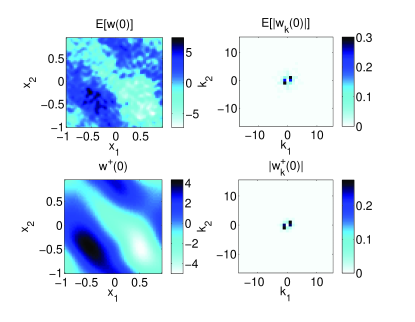
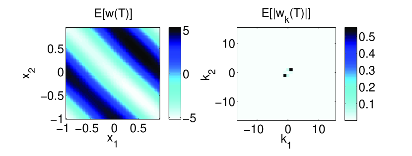
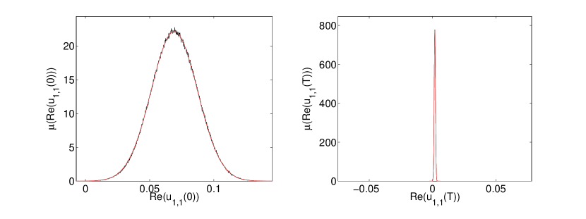
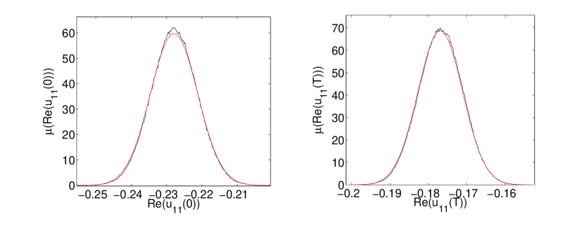
In the stationary regime, , the basic time-step used is , the smallest considered is , and we fix as the filtering time at which to make comparisons of the approximate filters with the moments of the posterior distribution via samples from MCMC, the MAP estimator from 4DVAR, the truth, and the observations. Figure 1 shows the vorticity, (left), and Fourier coefficients, (right), of the smoothing distribution at in the case that . The top panels are the mean of the posterior distribution found with MCMC, (, and the bottom panels are the truth, . The MAP estimator (minimizer of , ) is not shown because it is not discernable from the mean in this case. Notice that the mean (and MAP estimator) on the initial condition resemble the large-scale structure of the truth, but are more rough. This roughness is caused by the presence of the prior mean drawn according to the distribution . The solution operator immediately removes this roughness as it damps high wavenumbers; this effect can be seen in the images of the smoothing distribution mapped forward to time , i.e. the filtering distribution, in Figure 2 ( here only the mean is shown, as neither the truth nor the MAP estimator are distinguishable from it). This is apparent in the data in the tables discussed below, in which the distance between the truth, the posterior distribution, and the MAP estimator are all mutually much closer for the final time than the initial; this contraction of the errors in time is caused by the underlying dynamics which involves exponential attraction to a unique stationary state. This is further exihibited in Figure 3 which shows the histogram of the smoothing distribution for the real part of a sample mode, , at the initial time (left) and final time (right).
Table 1 presents data for increasing , with fixed. Notable trends, in addition to those mentioned at the start of this section, are as follows: (i) the 4DVAR smoothing distribution has much smaller error with respect to the mean at than at , with the former increasing and the latter decreasing for increasing ; the error of 4DVAR with respect to the mean and the variance at and are close to or below the threshold of accuracy of MCMC; (iii) the error of both the mean and the variance of 3DVAR tend to decrease with increasing ;
d Strongly Chaotic Regime
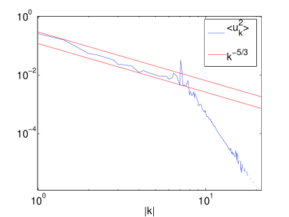
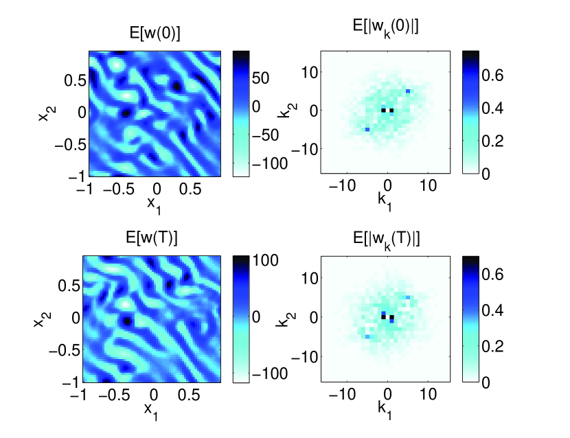
In the strongly chaotic regime, , the basic time-step used is , the smallest considered is , and we fix or as the filtering time at which to make comparisons of the approximate filters. In this regime, the dynamics are significantly more nonlinear and less predictable, with a high-dimensional attractor spanning many scales. Indeed the energy spectrum decays like for , with the magnitude of the forcing wavenumber, and much more rapidly for . See the left panel of Figure 4 for the average spectrum of the solution on the attractor and Fig. 5 for an example snapshot of the solution on the attractor. The flow is not in any of the classical regimes of cascades, but there is an upscale transfer of energy because of the forcing at intermediate scale. The viscosity is not negligible even at the largest scales, thereby allowing statistical equilibrium; this may be thought of as being generated by the empirical measure on the global attractor whose existence is assured for all . We confirmed this with simulations to times of order giving samples with which to compute the converged correlation statistics used in FDF.
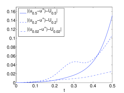
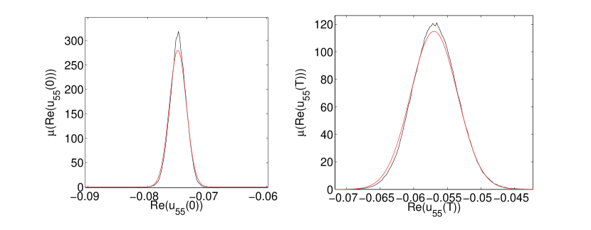
Small perturbations in the directions of maximal growth of the dynamics grow substantially over the larger times between observations we look at, while over the shorter times the dynamics remain well approximated by the linearization. See the right panel of Figure 4 for an example of the local maximal growth of perturbations. Figure 5 shows the initial and final time profiles of the mean as in Figures 1 and 2. Now that the solutions themselves are more rough, it is not possible to notice the influence of the prior mean at , and the profiles of the truth and MAP are indistinguishable from the mean throughout the interval of time. The situation in this regime is significantly different from the situation close to a stationary solution, primarily because the dimension of the attractor is very large and the dynamics on it are very unpredictable. Notice in Figure 6 (top) that the uncertainty in now barely decreases as we pass from initial time to final time . Indeed for moderately high modes, the uncertainty increases (see 6 (bottom) for the distribution of ).
Table 2 presents data for increasing , with fixed. Table 3 shows data for increasing with fixed. Notable trends, in addition to those mentioned at the start of the section, are: (i) when computable, the variance of the 4DVAR smoothing distribution has smaller error at than at ; (ii) the 4DVAR smoothing distribution error with respect to the variance cannot be computed accurately for because of accumulated error for long times in the aproximation of the adjoint of the forward operator by the discretization of the analytical adjoint; (iii) the error of 4DVAR with respect to the mean at for is below the threshold of accuracy of MCMC; (iv) the error in the variance for the FDF algorithm is very large because the is an order of magnitude larger than ; (v) the FDF algorithm is consistent in recovering the mean for increasing , while the other algorithms deteriorate; (vi) the error of FDF with respect to the variance decreases with increasing ; (vii) for and the FDF performs best and these desirable properties of the FDF variant on 3DVAR are associated with stability and will be discussed in the next section; (viii) for increasing , the error in the mean of LRExKF increases first when and and becomes close to the error in the variance which can be explained by the bias induced by neglecting the next order of the expansion of the dynamics; (ix) the error in LRExKF is substantial when and it really majorly fails when which is consistent with the time-scale on which nonlinear effects become prominent (see Fig. 4) and the linear approximation would not be expected to be valid. The error in the mean is larger, again as expected from the Ito correction term.
| MCMC() | 0 | 0 | 0.17177 | 0.819094 | 0.00153443 |
| 4DVAR() | 0.00153523 | 0.00620345 | 0.185876 | 0.740612 | 0 |
| MCMC() | 0 | 0 | 0.0164605 | 0.558026 | 5.17207e-05 |
| 4DVAR() | 5.1723e-05 | 0.00459055 | 0.0164618 | 0.558024 | 0 |
| 3DVAR | 0.138652 | 108.516 | 0.13738 | 0.54585 | 0.138646 |
| FDF | 0.00173093 | 0.423299 | 0.0153513 | 0.558228 | 0.00172455 |
| LRExKF | 6.34566e-05 | 0.00320937 | 0.0164796 | 0.558022 | 2.22202e-05 |
| EnKF | 0.00359669 | 0.119076 | 0.0158585 | 0.558032 | 0.00362309 |
| truth () | 0.17177 | - | 0 | 0.816333 | 0.156072 |
| truth () | 0.0164605 | - | 0 | 0.713754 | 0.0164342 |
| MCMC() | 0 | 0 | 0.295424 | 0.791832 | 0.00110927 |
| 4DVAR() | 0.00110969 | 0.00375462 | 0.333225 | 0.748439 | 0 |
| MCMC() | 0 | 0 | 0.028831 | 0.662342 | 0.00016539 |
| 4DVAR() | 0.000165408 | 0.00896381 | 0.0287779 | 0.662373 | 0 |
| 3DVAR | 0.128956 | 41.6646 | 0.139419 | 0.646462 | 0.128929 |
| FDF | 0.00400194 | 0.458239 | 0.031512 | 0.654203 | 0.00403853 |
| LRExKF | 0.000165666 | 0.00267976 | 0.0287787 | 0.65413 | 1.84537e-05 |
| EnKF | 0.00289635 | 0.122461 | 0.0301991 | 0.654205 | 0.00285458 |
| truth () | 0.295424 | - | 0 | 0.780891 | 0.27957 |
| truth () | 0.028831 | - | 0 | 0.77011 | 0.0287068 |
| MCMC() | 0 | 0 | 0.32043 | 0.747756 | 0.000965003 |
| 4DVAR() | 0.000965294 | 0.00384239 | 0.357404 | 0.633977 | 0 |
| MCMC() | 0 | 0 | 0.03871 | 0.68846 | 0.000208273 |
| 4DVAR() | 0.000208299 | 0.00250571 | 0.0386606 | 0.68846 | 0 |
| 3DVAR | 0.105535 | 35.9905 | 0.108918 | 0.684345 | 0.10548 |
| FDF | 0.00177839 | 0.475338 | 0.0387006 | 0.688477 | 0.00173164 |
| LRExKF | 0.0002106 | 0.00272041 | 0.0386602 | 0.68846 | 2.991e-06 |
| EnKF | 0.00319756 | 0.106976 | 0.0385305 | 0.688464 | 0.00312047 |
| truth () | 0.32043 | - | 0 | 0.771936 | 0.299957 |
| truth () | 0.03871 | - | 0 | 0.688664 | 0.038578 |
5 Filter Stability
Many of the accuracy results for the filters described in the previous section are degraded if, as is common practice in applied scenarios, modifications are made to ensure that the algorithms remain stable over longer time-intervals; that is if some form of variance inflation is performed to keep the algorithm close to the true signal, or to prevent it from suffering filter divergence (see Jazwinski (1970), Fisher et al. (2005), Evensen (2009), and references therein). In this section we describe some of the mathematics which underlies stabilization, describe numerical results illustrating it, and investigate its effect on filter accuracy. The basic conclusion of this section is that stabilization via variance inflation enables algorithms to be run for longer time windows before diverging, but may cause poorer accuracy in both the mean (before divergence) and the variance predictions. Again, we make no claims of optimal implementation of these filters, but rather aim to describe the mechanism of stabilization and the common effect, in general, as measured by ability to reproduce the gold standard posterior distribution.
We define stability in this context to mean that the distance between the truth and the estimated mean remains small. As we will demonstrate, whether or not this distance remains small depends on whether the observations made are sufficient to control any instabilities inherent in the model dynamics. To understand this issue it is instructive to consider the 3DVAR, FDF and LRExKF filters, all of which use a prediction step (13) which updates the mean using . When combined with the data incorporation step (11) we get an update equation of the form
| (18) |
where is the Kalman gain matrix. If we assume that the data is derived from a true signal satisfying and that
where the denote the observation errors, then we see that (18) has the form
| (19) |
If the observational noise is assumed to be consistent with the model used for the assimilation, then are i.i.d. random variables and we note that (19) is an inhomogenous Markov chain.
Note that
| (20) |
so that defining the error and subtracting (20) from (19) we obtain the equation
where The stability of the filter will be governed by families of products of the form
We observe that will act to induce stability, as it has norm less than one in appropriate spaces; , however, will induce some instability whenever the dynamics themeslves contain unstable growing modes. The balance between these effects – stabilization through observation and instability in the dynamics – determines whether the overall algorithm is stable.
The operator weights the relative importance of the model and the observations, according to covariance information. Therefore, this weighting must effectively stabilize the growing directions in the dynamics. Note that increasing – variance inflation – has the effect of moving towards the identity, so the mathematical mechanism of controlling the instability mechanism by variance inflation is elucidated by the discussion above. In particular, when the assimilation is proceeding in a stable fashion, the modes in which growing directions have support typically overestimate the variance to induce this stability. In unstable cases, there are at least some times at which some modes in which growing directions have support underestimate the variance, leading to instability of the filter. It is always the case that the onset of instability occurs when the distance from the estimated mean to the truth persistently exceeds the estimated standard deviation. In Brett et al. (2010) we provide the mathematical details and rigorous proofs which underpin the preceding discussion.
In the following, two observations concerning the size of the error are particularly instructive. Firstly, using the distribution assumed on the , the following lower bound on the error is immediate444Here denotes expectation with respect to the random variables .:
| (21) |
This implies that the average scale of the error of the filter, with respect to the truth, is set by the scale of the observation error, and shows that the choice of the covariance updates, and hence the Kalman gain , will affect the exact size of the average error, on this scale. The second observation follows from considering the trivial “filter” obtained by setting which corresponds to simply setting so that all weight is placed on the observations. In this case the average error is equal to
| (22) |
As we would hope that incorporation of the model itself improves errors we view (22) as providing an upper bound on any reasonable filter and we will consider the filter “unstable” if the squared error from the truth exceeds . Thus we use (22) and (21) as guiding upper and lower bounds when studying the errors in the filter means in what follows.
In cases where our basic algorithm is unstable in the sense just defined we will also implement a stabilized algorithm, by adopting the commonly used practice of variance inflation. The discussion above demonstrates how this acts to induce stability by causing the to move closer to the identity. For 3DVAR this is achieved by taking the original and redefining it via the transformation . In all the numerical computations presented in this paper which concern the stabilized version of 3DVAR we take The FDF(b) algorithm remains stable since it already has an inflated variance via the model error term. For LRExKF we achieve variance inflation by replacing the perturbation term of Equation 16 with , where is the covariance arising from FDF(b). Finally we discuss stabilization of the EnKF. This is achieved by taking the original ’s given by (17) and redefining them via the transformations , and with . The parameter prevents initial divergence, maintains stability with direct incremental inflation and provides rank correction. This is only one option out of a wide array of possible hueristically derived such transformations. For example, rank correction is often performed by some form of localization which preserves trace and eliminates long-range correlations, while our rank correction preserves long-range correlations and provides trace inflation. The point here is that our transformation captures the essential mechanism of stabilization by inflation which, again, is our objective.
We denote the stabilized versions of 3DVAR, LRExKF, and EnKF by [3DVAR], [LRExKF], and [EnKF]. Because FDF itself always remains stable we do not show results for a stabilized version of this algorithm. Note that we use ensembles in EnKF of equal size to the number of approximate eigenvectors in LRExKF, in order to ensure comparable work. This is always 100, except for large , when some of the largest 100 eigenvalues are too close to zero to maintain accuracy, and so fewer eigenvectors are used in LRExKF in these cases. Also, note again that we are looking for general features across methods and are not aiming to optimize the inflation procedure for any particular method.
Examples of an unstable instance of 3DVAR and the corresponding stabilized filter, [3DVAR], are depicted in Figures 8 and 9, respectively, with In this regime the dynamics are strongly chaotic. The first point to note is that both simulations give rise to an error which exceeds the lower bound (21); and that the unstable algorithm exceeds the desired bound (22), whilst the stabilized algorithm does not; note also that the stabilized algorithm output is plotted over a longer time-interval than the original algorithm. A second noteworthy point relates to the power of using the dynamical model: this is manifest in the bottom right panels of each figure, in which the trajectory of a high wavenumber mode, close to the forcing frequency, is shown. The assimilation performs remarkably well for the trajectory of this wavenumber relative to the observations in the stabilized case, owing to the high weight on the dynamics and stability of the dynamical model for that wavenumber. Examples of an unstable instance of LRExKF and the corresponding stabilized filter, [LRExKF], are depicted in Figures 10 and 11, respectively, with . The behaviour illustrated is very similar to that exhibited for 3DVAR and [3DVAR].
In the following tables we make a comparison between the original form of the filters and their stabilized forms, using the gold standard Bayesian posterior distribution as the desired outcome. Table 4 shows data for and with fixed. Tables 5 and 6 show data for and with fixed. We focus our discussion on the approximation of the mean. It is noteworthy that, on the shorter time horizon , the stabilized algorithms are less accurate with respect to the mean than their original counterparts, for both values of observation time ; this reflects a lack of accuracy caused by inflating the variance. As would be expected, however, this behaviour is reversed on longer time-intervals, as is shown when , relfecting enhanced stability cased by inflating the variance. Table 5 shows the case with , and the stabilized version of 3DVAR outperforms the original version, although the stabilized versions of EnKF and LRExKF are not as accurate as the original version. In Table 6, with and , the stabilized versions improve upon the original algorithms in all three cases. Furthermore, in Table 6, we also display the FDF showing that, without any stabilization, this outperforms the other three filters and their stabilized counterparts.
6 Conclusion
Incorporating noisy data into uncertain computational models presents a major challenge in many areas of the physical sciences, and in atmospheric modelling and NWP in particular. Data assimilation algorithms in NWP have had measurable positive impact on forecast skill. Nonetheless, assessing the ability of these algorithms to forecast uncertainty is more subtle. It is important to do so, however, especially as prediction is pushed to the limits of its validity in terms of time horizons considered, or physical processes modelled. In this paper we have proposed an approach to the evaluation of the ability of data assimilation algorithms to predict uncertainty. The cornerstone of our approach is to adopt a fully non-Gaussian Bayesian perspective in which the probability distribution of the system state over a time horizon, given data over that time horizon, plays a pivotal role: we contend that algorithms should be evaluated by their ability to reproduce this probability distribution, or important aspects of it, accurately.
In order to make this perspective useful it is necessary to find a model problem which admits complex behaviour reminiscent of atmospheric dynamics, whilst being sufficiently small to allow computation of the Bayesian posterior distribution, so that data assimilation algorithms can be compared against it. Although MCMC sampling of the posterior can, in principle, recover any distribution, it becomes prohibitively expensive for multi-modal distributions, depending on the energy barriers between modes. However for unimodal problems, state-of-the-art sampling techniques allow fully resolved MCMC computations to be undertaken. We have found that the 2D Navier-Stokes equations provide a model for which the posterior distribution may be accurately sampled using MCMC, in regimes where the dynamics is stationary and where it is strongly chaotic. We have confined our attention to strong constraint models, and implemented a range of variational and filtering methods, evaluating them by their ability to reproduce the Bayesian posterior distribution. The set-up is such that the Bayesian posterior is unimodal and approximately Gaussian. Thus the evaluation is undertaken by comparing the mean and covariance structure of the data assimilation algorithms against the actual Bayesian posterior mean and covariance. Similar studies were undertaken in the context of a subsurface geophysical inverse problem in Liu and Oliver (2003), although the conclusions were less definitive. It would be interesting to revisit such subsurface geophysical inverse problems using the state-of-the-art MCMC techniques adopted here, in order to compute the posterior distribution. Moreover it would be interesting to conduct a study, similar to that undertaken here, for models of atmospheric dynamics such as Lorenz-96, or a quasi-geostrophic models, which admit baroclinic instabilities.
These studies, under the assumption of a well-defined posterior probability distribution, lead to four conclusions: (i) most filtering and variational algorithms do a reasonably good job of reproducing the mean; (ii) for most of the filtering and variational algorithms studied and implemented here there are circumstances where the approximations underlying the ad hoc filters are not justified and they then fail to reproduce covariance information with any accuracy (iii) most filtering algorithms exhibit instability on longer time-intervals causing them to lose accuracy in even mean prediction; (iv) filter stabilization, via variance inflation of one sort or the other, ameliorates this instability and can improve long-term accuracy of the filters in predicting the mean, but can reduce the accuracy on short time intervals and of course makes it impossible to predict the covariance. In summary most data assimilation algorithms used in practice should be viewed with caution when using them to make claims concerning uncertainty although, when properly tuned, they will frequently track the signal mean accurately for fairly long time intervals. These conclusions are intrinsic to the algorithms, and result from the nature of the approximations made in order to create tractable online algorithms; the basic conclusions are not expected to change by use of different dynamical models, or by modifying the parameters of those algorithms.
Finally we note that we have not addressed in this paper the important but complicated issue of how to choose the prior distribution on the initial condition. We finish with some remarks concerning this. The “accuracy of the spread” of the prior is often monitored in practice with a rank histogram Anderson (1996). This can be computed even in the absence of an ensemble for any method in the class of those discussed here, by partitioning the real line in bins according to the assumed Gaussian prior density. It is important to note that uniform component-wise rank histograms in each direction guarantee that there are no directions in which the variance is consistently underestimated, and this should therefore be sufficient for stability. It is also necessary for the accurate approximation of the Bayesian posterior distribution, but by no means sufficient Hamill et al. (2000). Indeed, one can iteratively compute a constant prior with the cycled 3DVAR algorithm Hamill et al. (2000) such that the estimator from the algorithm will have statistics consistent with the constant prior used in the algorithm. The estimator produced by this algorithm is guaranteed by construction to yield uniform rank histograms of the type described above, and yet the actual prior coming from the posterior at the previous time is not constant, so this cannot be a good approximation of the actual prior. See Fig. 7 for an image of the variance which is consistent with the statistics of the estimator over iterations of 3DVAR with and , as compared with the prior, posterior, and converged FDF variance at . Notice FDF overestimates in the high-variance directions, and underestimates in the low-variance directions (which correspond in our case to the unstable and stable directions, respectively). The RMSE of 3DVAR with constant converged FDF variance is smaller than with constant variance from converged statistics, and yet the former clearly will yield component-wise rank histograms which appear to always underestimate the “spread” in the low-variance, stable directions, and overestimate in the high-variance, unstable directions. It is also noteworthy that the FDF variance accurately recovers the decay of the posterior variance, but is about an order of magnitude larger. Further investigation of how to initialize statistical forecasting algorithms clearly remains a subject presenting many conceptual and practical challenges.
| MCMC() | 0 | 0 | 0.0331468 | 0.337233 | 0.000731645 |
| 4DVAR() | 0.000731491 | 0.0932748 | 0.0331531 | 0.310411 | 0 |
| MCMC() | 0 | 0 | 0.0423943 | 0.32224 | 0.00130105 |
| 4DVAR() | 0.00130112 | 0.045048 | 0.042431 | 0.322306 | 0 |
| 3DVAR | 0.0634553 | 6.34057 | 0.063289 | 0.321959 | 0.0634026 |
| FDF | 0.165732 | 28.9155 | 0.175397 | 0.307159 | 0.165844 |
| LRExKF | 0.00599214 | 0.030054 | 0.0416529 | 0.322277 | 0.0054415 |
| EnKF | 0.035271 | 0.274428 | 0.0523566 | 0.323074 | 0.0354624 |
| truth () | 0.0331468 | - | 0 | 0.335933 | 0.0361395 |
| truth () | 0.0423943 | - | 0 | 0.339539 | 0.0429021 |
| MCMC() | 0 | 0 | 0.0496982 | 0.294743 | 0.000815864 |
| 4DVAR() | 0.000815762 | 0.0287498 | 0.0497009 | 0.280425 | 0 |
| MCMC() | 0 | 0 | 0.0698665 | 0.35798 | 0.00306996 |
| 4DVAR() | 0.00307105 | 0.0118785 | 0.06983 | 0.358094 | 0 |
| 3DVAR | 0.159393 | 2.2339 | 0.203165 | 0.374188 | 0.159658 |
| FDF | 0.200044 | 13.259 | 0.215136 | 0.308921 | 0.200045 |
| LRExKF | 0.023073 | 0.0313686 | 0.0766505 | 0.357915 | 0.0215118 |
| EnKF | 0.0539001 | 0.174878 | 0.109402 | 0.358301 | 0.0543726 |
| truth () | 0.0496982 | - | 0 | 0.303742 | 0.0541391 |
| truth () | 0.0698665 | - | 0 | 0.368335 | 0.0705546 |
| MCMC() | 0 | 0 | 0.0459125 | 0.293686 | 0.00122936 |
| 4DVAR() | 0.00183617 | 0.0231955 | 0.0462013 | 0.281137 | 0 |
| MCMC() | 0 | 0 | 0.072738 | 0.352456 | 0.00385795 |
| 4DVAR() | 0.00386162 | 0.0196227 | 0.0723178 | 0.352145 | 0 |
| 3DVAR | 0.285461 | 1.72154 | 0.300853 | 0.38443 | 0.286161 |
| FDF | 0.202274 | 10.7793 | 0.203287 | 0.316707 | 0.202862 |
| LRExKF | 0.0750908 | 0.0547417 | 0.0886932 | 0.35073 | 0.0726792 |
| EnKF | 0.0964053 | 0.0948967 | 0.113806 | 0.352625 | 0.0962341 |
| truth () | 0.0459125 | - | 0 | 0.301899 | 0.0496251 |
| truth () | 0.072738 | - | 0 | 0.368331 | 0.0720492 |
| MCMC() | 0 | 0 | 0.0322397 | 0.294722 | 0.00122667 |
|---|---|---|---|---|---|
| 4DVAR() | 0.00122657 | - | 0.0316494 | 0.280742 | 0 |
| MCMC() | 0 | 0 | 0.0480924 | 0.27997 | 0.00484999 |
| 4DVAR() | 0.0048519 | - | 0.0474821 | 0.279995 | 0 |
| 3DVAR | 0.35571 | 3.17803 | 0.357351 | 0.419614 | 0.35557 |
| FDF | 0.141426 | 19.2983 | 0.152064 | 0.260197 | 0.142169 |
| LRExKF | 0.101179 | 0.28308 | 0.0900697 | 0.291704 | 0.101287 |
| EnKF | 0.202724 | 0.230518 | 0.173947 | 0.320302 | 0.202665 |
| truth () | 0.0322397 | - | 0 | 0.303376 | 0.0272922 |
| truth () | 0.0480924 | - | 0 | 0.281553 | 0.0474964 |
| MCMC() | 0 | 0 | 0.0318531 | 0.293871 | 0.0030989 |
| 4DVAR() | 0.00309769 | - | 0.0313382 | 0.280152 | 0 |
| MCMC() | 0 | 0 | 0.0460821 | 0.288812 | 0.00831516 |
| 4DVAR() | 0.00831886 | - | 0.0448424 | 0.289043 | 0 |
| 3DVAR | 0.458527 | 1.8214 | 0.45353 | 0.487658 | 0.460144 |
| FDF | 0.189832 | 11.4573 | 0.19999 | 0.25111 | 0.191364 |
| LRExKF | 0.644427 | 0.325391 | 0.650004 | 1.22145 | 0.646233 |
| EnKF | 0.901703 | 0.554611 | 0.895878 | 0.908817 | 0.902438 |
| truth () | 0.0318531 | - | 0 | 0.303185 | 0.0269929 |
| truth () | 0.0460821 | - | 0 | 0.294524 | 0.0448046 |
Acknowledgments.
Both authors are grateful to the referees for numerous suggestions which have improved the presentation of this material; In particular, we thank Chris Snyder. KJHL is grateful to the EPSRC for funding. AMS is grateful to EPSRC, ERC and ONR for funding.
7 Appendix: Some numerical details
Here we provide some details of the numerical algorithms underlying the computations which we present in the main body of the paper. First, we will describe the numerical methods used for the dynamical model. Secondly we study the adjoint solver. Thirdly we discuss various issues related to the resulting optimization problems and large linear systems encountered. Finally we discuss the MCMC method used to compute the gold standard posterior probability distribution.
In the dynamical and observational models the forcing in Eq. 1 is taken to be , where and with the canonical skew-symmetric matrix, and for stationary () regime, while for the strongly chaotic regime in order to allow an upscale cascade of energy. Furthermore, we set the observational noise to white noise , where is chosen as 10% of the maximum standard deviation of the strongly chaotic dynamics, and we choose an initial smoothness prior , where is the Stokes operator. We notice that only the observations on the unstable manifold of the underlying solution map need to be assimilated. A similar observation was made in Chorin and Krause (2004) in the context of particle filters. Our choice of prior and observational covariance reflect this in the sense that the ratio of the prior to the observational covariance is larger for smaller wavenumbers (and greater than 1, in particular), in which the unstable manifold has support, while this ratio tends to zero as . The initial mean, or background state, is chosen as , where is the true initial condition. In the case of strongly chaotic dynamics it is taken as an arbitrary point on the attractor obtained by simulating an arbitrary initial condition until statistical equilibrium. The initial condition for the case of stationary dynamics is taken as a draw from the Gaussian prior, since the statistical equilibrium is the trivial one.
Our numerical method for the dynamical model is based on a Galerkin approximation of the velocity field in a divergence-free Fourier basis. We use a modification of a fourth-order Runge-Kutta method, ETD4RK Cox and Matthews (2002), in which the heat semi-group is used together with Duhamel’s principle to solve exactly for the diffusion term. A spectral Galerkin method Hesthaven et al. (2007) is used in which the convolutions arising from products in the nonlinear term are computed via FFTs. We use a double-sized domain in each dimension, buffered with zeros, resulting in grid-point FFTs, and only half the modes are retained when transforming back into spectral space in order to prevent de-aliasing which is avoided as long as fewer than 2/3 the modes are retained. Data assimilation in practice always contends with poor spatial resolution, particularly in the case of the atmosphere in which there are many billions of degrees of freedom. For us the important resolution consideration is that the unstable modes, which usually have long spatial scales and support in low wave-numbers, are resolved. Therefore, our objective here is not to obtain high spatial-resolution but rather to obtain high temporal-resolution in the sense of reproducibility. We would like the divergence of two close-by trajectories to be dictated by instability in the dynamical model rather than the numerical time-stepping scheme.
It is also important that we have accurate adjoint solvers, and this is strongly linked to the accuracy of the forward solver. The same time-stepper is used to solve the adjoint equation, with twice the time-step of the forward solve, since the forward solution is required at half-steps in order to implement this method for the non-autonomous adjoint solve. Many issues can arise in the implementation of adjoint, or costate methods Banks (1992); Vogel and Wade (1995) and the practitioner should be aware of these. The easiest way to ensure convergence is to test that the tangent linearized map is indeed the linearization of the solution map and then confirm that the adjoint is the adjoint to a suitable threshold. We have taken the approach of “optimize then discretize” here, and as such our adjoint model is the discretization of the analytical adjoint. This effect becomes apparent in the accuracy of the linearization for longer time intervals, and we are no longer able to compute accurate gradients and Hessians as a result.
Regarding linear algebra and optimization issues we make the following observations. A Krylov method (GMRES) is used for linear solves in the Newton method for 4DVAR, and the Arnoldi method is used for low-rank covariance approximations in LRExKF and for the filtering time covariance approximation in 4DVAR. The LRExKF always sufficiently captures more than of the full rank version as measured in Frobenius (matrix ) norm. The initial Hessian in 4DVAR and well as the ones occuring within Newton’s method are computed by finite difference. Using a gradient flow (preconditioned steepest descent) computation, we obtain an approximate minimizer close to the actual minimizer and then a preconditioned Newton-Krylov nonlinear fixed-point solver is used (nsoli Kelley (2003)). This approach is akin to the Levenburgh-Marquardt algorithm. See Trefethen and Bau (1997) and Saad (1996) for overviews of the linear algebra and Nocedal and Wright (1999) for an overview of optimization. Strong constraint 4DVAR can be computationally challenging and, although we do not do so here, it would be interesting to study weak constraint 4DVAR from a related perspective; see Bröcker (2010) for a discussion of weak constraint 4DVAR in continuous time. It is useful to employ benchmarks in order to confirm gradients are being computed properly when implementing optimizers, see for example Lawless et al. (2003).
Finally, we comment on the MCMC computations which, of all the algorithms implemented here, lead to the highest computational cost. This, of course, is because it fully resolves the posterior distribution of interest whereas the other algorithms use crude approximations, the consequences of which we study by comparison with accurate MCMC results. Each time-step requires function evaluations, and each function evaluation requires FFTs, so it costs FFTs for each time-step. We fix the lengths of paths at time-steps for most of the computations, but nonetheless, this is on the order of FFTs per evaluation of the dynamical model. If a FFT takes ms, then this amounts to s per sample. Clearly this is a hurdle as it would take on the order of days to obtain on the order of millions of samples in serial. We overcome this by using the MAP estimator (4DVAR solution) as the initial condition in order to accellerate burn-in, and then run independent batches of samples in parallel with independent seeds in the random number generator. We also minimize computional effort within the method by employing the technique of early rejection introduced by Haario (2010) which means that rejection can be detected before the forward computation required for evaluation of reaches the end of the assimilation time window; the computation can then be stopped and hence computational savings made.
It is important to recognize that we cannot rely too heavily on results of MCMC with smaller relative norm than for the mean or for the variance, because we are bound to convergence and it is already prohibitively expensive to get several million samples. More than is not tractable. Convergence is measured by a version of MSPRF Brooks and Gelman (1998), , where corresponds to sample statistics with chain and corresponds to sample statistics over chains. We find for samples in each chain. If we define , then we have .
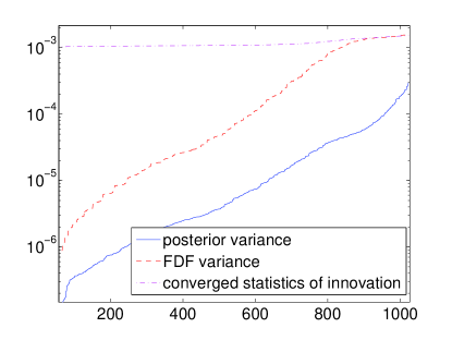
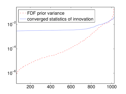
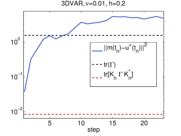
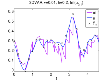
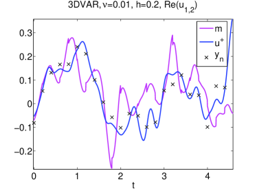
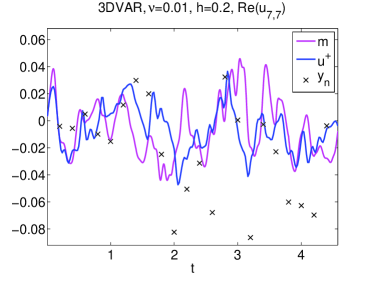
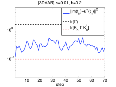
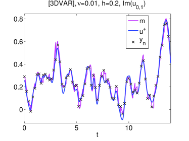
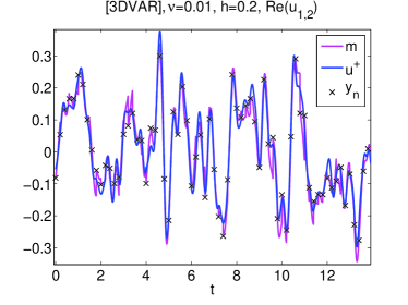
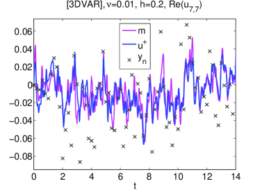
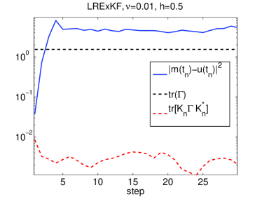
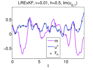
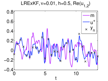
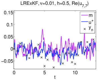
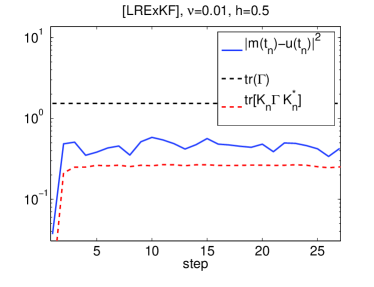
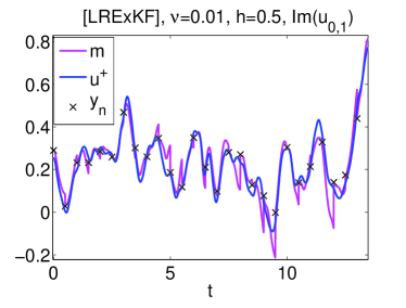
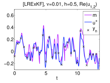
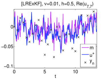
| h=0.02 | |||||
|---|---|---|---|---|---|
| 3DVAR | 0.0634553 | 6.34057 | 0.063289 | 0.321959 | 0.0634026 |
| [3DVAR] | 0.142759 | 22.2668 | 0.153141 | 0.309838 | 0.143005 |
| EnKF | 0.035271 | 0.274428 | 0.0523566 | 0.323074 | 0.0354624 |
| [EnKF] | 0.167776 | 28.1196 | 0.175359 | 0.304352 | 0.167919 |
| h=0.2 | |||||
| 3DVAR | 0.285461 | 1.72154 | 0.300853 | 0.38443 | 0.286161 |
| [3DVAR] | 0.195222 | 6.33608 | 0.204883 | 0.339108 | 0.196339 |
| LRExKF | 0.0750908 | 0.0547417 | 0.0886932 | 0.35073 | 0.0726792 |
| [LRExKF] | 0.156973 | 7.64123 | 0.169354 | 0.310298 | 0.156596 |
| EnKF | 0.137844 | 0.372259 | 0.159744 | 0.353934 | 0.137969 |
| [EnKF] | 0.248081 | 6.34903 | 0.267746 | 0.368067 | 0.249475 |
| h=0.2 | |||||
|---|---|---|---|---|---|
| 3DVAR | 0.35571 | 3.17803 | 0.357351 | 0.419614 | 0.35557 |
| [3DVAR] | 0.131964 | 11.5997 | 0.135572 | 0.277895 | 0.133265 |
| LRExKF | 0.101179 | 0.28308 | 0.0900697 | 0.291704 | 0.101287 |
| [LRExKF] | 0.12962 | 16.3692 | 0.13592 | 0.256617 | 0.129742 |
| EnKF | 0.0736613 | 0.276947 | 0.0755232 | 0.282247 | 0.0742144 |
| [EnKF] | 0.1231 | 14.8557 | 0.133171 | 0.261061 | 0.124203 |
| h=0.5 | |||||
|---|---|---|---|---|---|
| 3DVAR | 0.458527 | 1.8214 | 0.45353 | 0.487658 | 0.460144 |
| [3DVAR] | 0.27185 | 6.62328 | 0.285351 | 0.307263 | 0.274663 |
| LRExKF | 0.644427 | 0.325391 | 0.650004 | 1.22145 | 0.646233 |
| [LRExKF] | 0.201327 | 11.2449 | 0.207526 | 0.244101 | 0.201081 |
| EnKF | 0.901703 | 0.554611 | 0.895878 | 0.908817 | 0.902438 |
| [EnKF] | 0.169262 | 4.07238 | 0.17874 | 0.244571 | 0.170245 |
| FDF | 0.189832 | 11.4573 | 0.19999 | 0.25111 | 0.191364 |
REFERENCES
- Anderson (1996) Anderson, J., 1996: A method for producing and evaluating probabilistic forecasts from ensemble model integrations. Journal of Climate, 9 (7), 1518–1530.
- Apte et al. (2007) Apte, A., M. Hairer, A. Stuart, and J. Voss, 2007: Sampling the posterior: an approach to non-Gaussian data assimilation. Physica D, 230, 50–64.
- Apte et al. (2008a) Apte, A., C. Jones, and A. Stuart, 2008a: A Bayesian approach to Lagrangian data assimilation. Tellus, 60, 336–347.
- Apte et al. (2008b) Apte, A., C. Jones, A. Stuart, and J. Voss, 2008b: Data assimilation: Mathematical and statistical perspectives. International Journal for Numerical Methods in Fluids, 56 (8), 1033–1046.
- Arulampalam et al. (2002) Arulampalam, M., S. Maskell, N. Gordon, and T. Clapp, 2002: A tutorial on particle filters for online nonlinear/non-gaussian bayesian tracking. Signal Processing, IEEE Transactions on, 50 (2), 174–188.
- Auvinen et al. (2009) Auvinen, H., J. Bardsley, H. Haario, and T. Kauranne, 2009: Large-scale kalman filtering using the limited memory bfgs method. Electronic Transactions on Numerical Analysis, 35, 217–233.
- Bain and Crişan (2008) Bain, A. and D. Crişan, 2008: Fundamentals of stochastic filtering. Springer Verlag.
- Banks (1992) Banks, H., 1992: Computational issues in parameter estimation and feedback control problems for partial differential equation systems. Physica D: Nonlinear Phenomena, 60 (1-4), 226–238.
- Banks and Kunisch (1989) Banks, H. and K. Kunisch, 1989: Estimation techniques for distributed parameter systems. Birkhauser Boston.
- Bengtsson et al. (2003) Bengtsson, T., C. Snyder, and D. Nychka, 2003: Toward a nonlinear ensemble filter for high-dimensional systems. J. Geophys. Res, 108 (D24), 8775.
- Bennett (2002) Bennett, A., 2002: Inverse Modeling of the ocean and Atmosphere. Cambridge.
- Brett et al. (2010) Brett, C., A. Lam, K. Law, D. McCormick, M. Scott, and A. Stuart, 2010: Stability of filters for the navier-stokes equation. preprint.
- Bröcker (2010) Bröcker, J., 2010: On variational data assimilation in continuous time. Quarterly Journal of the Royal Meteorological Society, 136 (652), 1906–1919.
- Brooks and Gelman (1998) Brooks, S. and A. Gelman, 1998: General methods for monitoring convergence of iterative simulations. Journal of Computational and Graphical Statistics, 7 (4), 434–455.
- Bryson and Frazier (1963) Bryson, A. and M. Frazier, 1963: Smoothing for linear and nonlinear dynamic systems. Proceedings Optimum System Sythensis Conference, US Air Force Tech. Rep. AFB-TDR-63-119.
- Carrassi et al. (2008) Carrassi, A., M. Ghil, A. Trevisan, and F. Uboldi, 2008: Data assimilation as a nonlinear dynamical systems problem: Stability and convergence of the prediction-assimilation system. Chaos: An Interdisciplinary Journal of Nonlinear Science, 18, 023 112.
- Chorin and Krause (2004) Chorin, A. and P. Krause, 2004: Dimensional reduction for a bayesian filter. Proceedings of the National Academy of Sciences of the United States of America, 101 (42), 15 013.
- Chorin et al. (2010) Chorin, A., M. Morzfeld, and X. Tu, 2010: Iimplicit particle filters for data assimilation. Communications in Applied Mathematics and Computational Science, 221.
- Cotter et al. (2009) Cotter, S., M. Dashti, J. Robinson, and A. Stuart, 2009: Bayesian inverse problems for functions and applications to fluid mechanics. Inverse Problems, 25, 115 008.
- Cotter et al. (2011) Cotter, S., M. Dashti, and A. Stuart, 2011: Variational data assimilation using targetted random walks. Int. J. Num. Meth. Fluids.
- Courtier and Talagrand (1987) Courtier, P. and O. Talagrand, 1987: Variational assimilation of meteorological observations with the adjoint vorticity equation. ii: Numerical results. Quarterly Journal of the Royal Meteorological Society, 113 (478), 1329–1347.
- Cox (1964) Cox, H., 1964: On the estimation of state variables and parameters for noisy dynamic systems. Automatic Control, IEEE Transactions on, 9 (1), 5–12.
- Cox and Matthews (2002) Cox, S. and P. Matthews, 2002: Exponential time differencing for stiff systems. Journal of Computational Physics, 176 (2), 430–455.
- Doucet et al. (2001) Doucet, A., N. De Freitas, and N. Gordon, 2001: Sequential Monte Carlo methods in practice. Springer Verlag.
- Evensen (2003) Evensen, G., 2003: The ensemble kalman filter: Theoretical formulation and practical implementation. Ocean dynamics, 53 (4), 343–367.
- Evensen (2009) Evensen, G., 2009: Data assimilation: the ensemble Kalman filter. Springer Verlag.
- Evensen et al. (1994) Evensen, G., P. Van Leeuwen, et al., 1994: Assimilation of geosat altimeter data for the agulhas current using the ensemble kalman filter with a quasi-geostrophic model. Monthly Weather.
- Fisher et al. (2005) Fisher, M., M. Leutbecher, and G. Kelly, 2005: On the equivalence between kalman smoothing and weak-constraint four-dimensional variational data assimilation. Quarterly Journal of the Royal Meteorological Society, 131 (613), 3235–3246.
- Haario (2010) Haario, H., 2010: Early rejection in metropolis-hastings. Private communication.
- Hamill et al. (2000) Hamill, T., C. Snyder, and R. Morss, 2000: A comparison of probabilistic forecasts from bred, singular-vector, and perturbed observation ensembles. Monthly Weather Review, 128 (6), 1835–1851.
- Harlim and Majda (2008) Harlim, J. and A. Majda, 2008: Filtering nonlinear dynamical systems with linear stochastic models. Nonlinearity, 21, 1281.
- Harvey (1991) Harvey, A., 1991: Forecasting, structural time series models and the Kalman filter. Cambridge Univ Pr.
- Hesthaven et al. (2007) Hesthaven, J., S. Gottlieb, and D. Gottlieb, 2007: Spectral methods for time-dependent problems, Vol. 21. Cambridge Univ Pr.
- Hinze et al. (2008) Hinze, M., R. Pinnau, M. Ulbrich, and S. Ulbrich, 2008: Optimization with PDE constraints. Springer Verlag.
- Jazwinski (1970) Jazwinski, A., 1970: Stochastic processes and filtering theory. Academic Pr.
- Kaipio and Somersalo (2005) Kaipio, J. and E. Somersalo, 2005: Statistical and computational inverse problems. Springer Science+ Business Media, Inc.
- Kalman (1960) Kalman, R., 1960: A new approach to linear filtering and prediction problems. Journal of basic Engineering, 82 (Series D), 35–45.
- Kalnay (2003) Kalnay, E., 2003: Atmospheric modeling, data assimilation, and predictability. Cambridge Univ Pr.
- Kelley (2003) Kelley, C., 2003: Solving nonlinear equations with Newton’s method, Vol. 1. Society for Industrial Mathematics.
- Lawless et al. (2003) Lawless, A., N. Nichols, and S. Ballard, 2003: A comparison of two methods for developing the linearization of a shallow-water model. Quarterly Journal of the Royal Meteorological Society, 129 (589), 1237–1254.
- Lei et al. (2010) Lei, J., P. Bickel, and C. Snyder, 2010: Comparison of ensemble kalman filters under non-gaussianity. Monthly Weather Review, 138 (4), 1293–1306.
- Leutbecher (2003) Leutbecher, M., 2003: Adaptive observations, the hessian metric and singular vectors. Proc. ECMWF Seminar on Recent developments in data assimilation for atmosphere and ocean, Reading, UK, 8–12.
- Liu and Oliver (2003) Liu, N. and D. S. Oliver, 2003: Evaluation of monte carlo methods for assessing uncertainty. SPE Journal, 8 (2), 188–195.
- Lorenc (1986) Lorenc, A., 1986: Analysis methods for numerical weather prediction. Quarterly Journal of the Royal Meteorological Society, 112 (474), 1177–1194.
- Lorenz (1963) Lorenz, E., 1963: Deterministic nonperiodic flow1. Atmos J Sci, 20, 130–141.
- Lorenz (1996) Lorenz, E., 1996: Predictability: A problem partly solved. Proc. Seminar on Predictability, Vol. 1, 1–18.
- Majda et al. (2010) Majda, A., J. Harlim, and B. Gershgorin, 2010: Mathematical strategies for filtering turbulent dynamical systems. DYNAMICAL SYSTEMS, 27 (2), 441–486.
- Meng and Zhang (2010) Meng, Z. and F. Zhang, 2010: Tests of an ensemble kalman filter for mesoscale and regional-scale data assimilation. part iv: Comparison with 3dvar in a month-long experiment.
- Miller et al. (1994) Miller, R., M. Ghil, and F. Gauthiez, 1994: Advanced data assimilation in strongly nonlinear dynamical systems. Journal of the Atmospheric Sciences, 51 (8), 1037–1037.
- Nocedal and Wright (1999) Nocedal, J. and S. Wright, 1999: Numerical optimization. Springer verlag.
- Palmer et al. (1998) Palmer, T., R. Gelaro, J. Barkmeijer, and R. Buizza, 1998: Singular vectors, metrics, and adaptive observations. Journal of the atmospheric sciences, 55 (4), 633–653.
- Quinn and Abarbanel (2010) Quinn, J. and H. Abarbanel, 2010: State and parameter estimation using monte carlo evaluation of path integrals. Quarterly Journal of the Royal Meteorological Society.
- Saad (1996) Saad, Y., 1996: Iterative methods for sparse linear systems. PWS Pub. Co.
- Snyder et al. (2008) Snyder, T., T. Bengtsson, P. Bickel, and J. Anderson, 2008: Obstacles to high-dimensional particle filtering. Monthly Weather Review., 136, 4629–4640.
- Stuart (2010) Stuart, A., 2010: Inverse problems: a Bayesian perspective. Acta Numerica, 19 (-1), 451–559.
- Talagrand and Courtier (1987) Talagrand, O. and P. Courtier, 1987: Variational assimilation of meteorological observations with the adjoint vorticity equation. i: Theory. Quarterly Journal of the Royal Meteorological Society, 113 (478), 1311–1328.
- Tarantola (2005) Tarantola, A., 2005: Inverse problem theory and methods for model parameter estimation. Society for Industrial Mathematics.
- Temam (2001) Temam, R., 2001: Navier-Stokes equations: theory and numerical analysis. Amer Mathematical Society.
- Tippett et al. (2003) Tippett, M., J. Anderson, C. Bishop, T. Hamill, and J. Whitaker, 2003: Ensemble square root filters. Monthly weather review, 131 (7), 1485–1490.
- Toth and Kalnay (1997) Toth, Z. and E. Kalnay, 1997: Ensemble forecasting at ncep and the breeding method. Monthly Weather Review, 125, 3297.
- Trefethen and Bau (1997) Trefethen, L. and D. Bau, 1997: Numerical linear algebra. 50, Society for Industrial Mathematics.
- Van Leeuwen (2009) Van Leeuwen, P., 2009: Particle filtering in geophysical systems. Monthly Weather Review, 137, 4089–4114.
- van Leeuwen (2010) van Leeuwen, P., 2010: Nonlinear data assimilation in geosciences: an extremely efficient particle filter. Quarterly Journal of the Royal Meteorological Society, 136 (653), 1991–1999.
- Vogel (2002) Vogel, C., 2002: Computational methods for inverse problems. Society for Industrial Mathematics.
- Vogel and Wade (1995) Vogel, C. and J. Wade, 1995: Analysis of costate discretizations in parameter estimation for linear evolution equations. SIAM journal on control and optimization, 33 (1), 227–254.
- Zhang and Zhang (2012) Zhang, M. and F. Zhang, 2012: E4dvar: Coupling an ensemble kalman filter with four-dimensional variational data assimilation in a limited-area weather prediction model. Monthly Weather Review-Boston, 140 (2), 587.
- Zhang et al. (2010) Zhang, M., F. Zhang, X. Huang, and X. Zhang, 2010: Inter-comparison of an ensemble kalman filter with three-and four-dimensional variational data assimilation methods in a limited-area model over the month of june 2003. Monthly Weather Review.
- Zupanski (1997) Zupanski, D., 1997: A general weak constraint applicable to operational 4dvar data assimilation systems. Monthly Weather Review, 125, 2274–2292.