3-D deconvolution of hyper-spectral astronomical data

Abstract

In this paper we present a general method for multichannel image restoration based on regularized $\chi^{2}$. We introduce separable regularizations that account for the dynamic of the model and take advantage of the continuities present in the data, leaving only two hyper-parameters to tune.

We illustrate a practical implementation of this method in the context of host galaxy subtraction for the Nearby SuperNova factory. We show that the image restoration obtained fulfills the stringent requirements on bias and photometricity needed by this program. The reconstruction yields sub-percent integrated residuals in all the synthetic filters considered both on real and simulated data.

Even though our implementation is tied to the SNfactory data, the method translates to any hyper-spectral data. As such, it is of direct relevance to several new generation instruments like MUSE. Also, this technique could be applied to multi-band astronomical imaging for which image reconstruction is important, for example to increase image resolution for weak lensing surveys.

1 Introduction

Multi-channel data usually refers to images of the same scene observed at multiple wavelengths, time frames, polarizations, etc. Data of this nature is involved in a wide range of applications such as remote sensing, biological and medical imaging, and of course astronomy. Because the light is spread out on multiple channels instead of being integrated on a single image, the information content of such data is increased at the cost of a lower signal to noise or achievable resolution for the same exposure time. Extracting the maximum of information from images in which each photon is acquired at a dear cost is thus a recurring concern for multi-channel imaging. All the techniques aiming toward this purpose, for example by removing the instrumental blur in order to recover a higher quality image, fall under the denomination of image restoration.

First attempts to restore multi-channel data made use of classical 2D restoration techniques like Wiener filter or Richardson-Lucy algorithms on each individual channel. The pitfall of these method is that they ignore the natural cross-channel correlations existing in the data. The first restoration technique specifically dedicated to multichannel data was introduced by Hunt & Kubler (1984). It proposed a MMSE restoration filter (Wiener filter) based on the assumption that the signal auto-correlation is spatially and spectrally separable. This assumption was later relaxed by Galatsanos & Chin (1989). Many other multichannel linear restoration filters Katsaggelos et al. (1993) have been proposed since, using Kalman filters (Tekalp & Pavlovic, 1990), adaptive 3D Wiener filter (Gaucel et al., 2006) or regularized least square (Galatsanos et al., 1991). More recently Benazza-Benyahia & Pesquet (2006) and Duijster et al. (2009) adapted a Fourier/Wavelet restoration technique ( ForWarD, Neelamani et al. (2004)) to multispectral data.

To enhance spatial resolution of multispectral data many authors (Hardie et al., 2004; Sroubek & Flusser, 2006; Molina et al., 2007; Vega et al., 2009, 2010) have proposed to merge spatial information contained in high resolution panchromatic images with the spectral information of low resolution hyper-spectral images. Based on this approach, a technique for spectral resolution enhancement has been proposed by Akgun et al. (2005) while Bobin et al. (2009) performs spatial resolution enhancement. His technique relies on the strong assumption that the scene observed is the linear combination of only a few materials with unknown spectrum.

As illustrated by these examples, most work on restoration of hyper-spectral images is done for remote sensing and color (RGB) images. Those methods can’t directly be applied to astronomical data because of its specific features like large dynamic range and strong sharp features (for example narrow emission lines). To the best of our knowledge, restoration techniques for hyper-spectral astronomical images have been proposed for slit spectrography data (Courbin et al., 2000; Lucy & Walsh, 2003) or data composed of slit spectrography scans with Spitzer (Rodet et al., 2008) but no such technique has been proposed for 3-D spectroscopy. By 3-D spectroscopy, we mean here i.e. $(\boldsymbol{\theta},\lambda)$ data observed simultaneously via an Integral Field Spectrograph (IFS) with $\boldsymbol{\theta}=(\theta_{1},\theta_{2})$ the 2-D angular position along the slit and $\lambda$ the wavelength.

Even though Schulz (1993) and following work present techniques of blind deconvolution of multi-frame data cubes, they don’t readily apply to 3-D spectroscopy. They are developed on sequences of short exposure images of turbulence-degraded observation of still object that have their own specificity compared to astronomical IFS data cubes. Maybe closer to the technique we propose here, Schultz & Stevenson (1995) discuss a method based on maximum a posteriori (MAP) spatial regularization with Hubber function. This approach is similar to ours in that they also propose a spatio-spectral weighting of their regularization. Nevertheless, their work targets color images very different from 3-D astronomical data.

Even among other astrophysical data, Integral Field Spectroscopy needs a specific approach. For example, WMAP CMB observations are multi-spectral images with 5 disjoint spectral bands, and display relatively smooth maps. On the other hand, IFS like SAURON, SNIFS, FLAMES+GIRAFFE, KMOS, WIFES, and in the future, MUSE observe simultaneously the spectra of whole regions of the sky, yielding $(\boldsymbol{\theta},\lambda)$ data cubes with several hundreds of wavelength bins. Each wavelength “slice” of such a cube is a mono-chromatic image at the resolution of the IFU spectrograph, and can display peaked spatial structures (like galactic cores and stars), as well as narrow emission or absorption lines. Dedicated image reconstruction techniques are needed to take full advantage of the data gathered by these instruments. The method presented in this paper positions itself in this context: it is very generic and exploits all the intrinsic continuities of hyper-spectral or data in order to yield the best image reconstruction possible.

In section 2 we describe the hyper-spectral mathematical model we wish to reconstruct. In section 3 we present the inverse problem approach we propose to achieve the hyper-spectral image restoration. In section 4 we present the specific context of the SuperNova factory in which our procedure is exemplified. Section 5 summarizes the algorithm implemented. Sections 6 and 7 show the result of our procedure both on simulated and real data, and Section 8 is dedicated to the discussion of the performance of the algorithm and of possible future improvements.

2 The Direct Model

In the following we describe how the model of the observed data relates to the specific intensity of the object of interest $I_{\mathsf{obj}}(\boldsymbol{\theta},\lambda)$, with $\boldsymbol{\theta}=(\theta_{1},\theta_{2})$ the 2-D position angle. The 3-D model of the observed data is a mixture of two components, the observed object (the scene) and the background, convolved by the point spread function (PSF) of the instrument.

$$I_{\mathsf{model}}(\boldsymbol{\theta},\lambda) =\iint\Bigl{[}I_{\mathsf{obj}}(\boldsymbol{\theta}^{\prime},\lambda)+I_{\mathsf{sky}}(\lambda)\Bigr{]}\,h(\boldsymbol{\theta}-\boldsymbol{\theta}^{\prime},\lambda)\,{\mathrm{d}\boldsymbol{\theta}^{\prime}}$$ (1)

with $I_{\mathsf{sky}}(\lambda)$ the specific intensity of the sky (assumed to be spatially uniform), $h(\boldsymbol{\theta},\lambda)$ the spatial point spread function (PSF). In order to simplify the equations, we will assume in what follows that we work on post processed data, for which dark current and spectral calibration have been properly handled.

In Eq. (1), we assume that there is no cross-talk between spectral channels, or that it has been properly accounted for at the CCD extraction level. Formally, we do not work with CCD 2D images on which the pixel location corresponds to a position and a wavelength, but with data cubes where the spectra have been properly extracted from the CCD and are labeled by their 2D position in the field of view. We also assume that the PSF is stationary (shift-invariant) which is appropriate for small fields of view. The PSF is not necessarily normalized in order to account for the variable throughput (atmospherical and instrumental transmission):

$$\eta(\lambda)=\iint h(\boldsymbol{\theta},\lambda)\,{\mathrm{d}\boldsymbol{\theta}}\,.$$ (2)

Similarly, the wavelength-wise PSF’s may be centered at a location $\boldsymbol{\theta}_{\lambda}$ which depends on the wavelength so as to account for imperfect instrumental alignment and atmospherical differential refraction (ADR). Finally, to conserve the physical units of the quantities of interest, the angular area of the pixel and the effective spectral bandwidth can also be integrated in the PSF.

Introducing the specific intensity of all background sources:

$$I_{\mathsf{bg}}(\lambda) =I_{\mathsf{sky}}(\lambda)\,\iint h(\boldsymbol{\theta},\lambda)\,{\mathrm{d}\boldsymbol{\theta}}$$ (3)

$$=\eta(\lambda)\,I_{\mathsf{sky}}(\lambda)$$ (4)

our model equation simplifies to:

$$I_{\mathsf{model}}(\boldsymbol{\theta},\lambda)=\iint I_{\mathsf{obj}}(\boldsymbol{\theta}^{\prime},\lambda)\,h(\boldsymbol{\theta}-\boldsymbol{\theta}^{\prime},\lambda)\,{\mathrm{d}\boldsymbol{\theta}^{\prime}}+I_{\mathsf{bg}}(\lambda)\,.$$ (5)

After background subtraction, the available data is a cube of quasi-monochromatic images that we can model as follows:

$${y_{j,\ell}}=\left[I_{\mathsf{model}}(\boldsymbol{\theta}_{j},{\lambda_{\ell}})-I_{\mathsf{bg}}({\lambda_{\ell}})\right]\,\Delta\theta_{j}^{2}\,\Delta{\lambda_{\ell}}+{e_{j,\ell}}$$ (6)

with $\boldsymbol{\theta}_{j}$ the angular direction of $j$-th image pixel, ${\lambda_{\ell}}$ the effective wavelength in $\ell$-th spectral channel, and ${e_{j,\ell}}$ an error term due to the noise and the model approximations. Multiplication by $\Delta\theta_{j}^{2}$, the area of $j$-th pixel, and by $\Delta{\lambda_{\ell}}$, the effective bandwidth of the $\ell$-th spectral channel, approximately takes into account the integration of the signal.

Without loss of generality, the continuous 3-D spatio-spectral distribution of the object we wish to reconstruct can be parametrized by a finite number of coefficients by means of expansion onto a basis of functions, for instance:

$$I_{\mathsf{obj}}(\boldsymbol{\theta},\lambda)=\sum_{k,\ell^{\prime}}{x_{k,\ell^{\prime}}}\,b_{\mathsf{spatial}}(\boldsymbol{\theta}-{\boldsymbol{\theta}^{\prime}_{k}})\,b^{\mathsf{spectral}}_{\ell^{\prime}}(\lambda)$$ (7)

with $\mathcal{G}_{\mathsf{spatial}}=\{{\boldsymbol{\theta}^{\prime}_{k}}\}_{k=1}^{N_{\Omega}^{\prime}}$ the grid of sampled angular positions in the synthesized field of view, $b_{\mathsf{spatial}}(\boldsymbol{\theta})$ the 2-D angular interpolation (or basis) function, $\mathcal{G}_{\mathsf{spectral}}=\{{\lambda^{\prime}_{\ell^{\prime}}}\}_{\ell^{\prime}=1}^{N_{\lambda}^{\prime}}$ the grid of sampled wavelengths and $b_{\mathsf{spectral}}(\lambda)$ the spectral interpolation (or basis) function. $N_{\Omega}^{\prime}$ is the number of pixels in the synthesized field of view and $N_{\lambda}^{\prime}$ is the number of spectral channels, or wavelength bins over which the object of interest is described. While the angular grid must be evenly spaced, this is not the case for the spectral grid. This could be used by tuning the grid to a finer resolution where sharp spectral features are expected. If the spectral grid is regular (as will be the case in our examples) the spectral interpolation function in Eq. (7) becomes $b^{\mathsf{spectral}}_{\ell^{\prime}}(\lambda)=b_{\mathsf{spectral}}(\lambda-{\lambda^{\prime}_{\ell^{\prime}}})$. Note also that in order to avoid edge effects such as field aliasing, the spatial grid must be larger than the observed field of view. This point will be addressed in more detail later on.

Using the parametrization of the object brightness distribution in Eq. (7) and the image model in Eq. (5), our model of the data writes:

$${y_{j,\ell}}=\sum_{k,\ell^{\prime}}{H_{j,\ell,k,\ell^{\prime}}}\,{x_{k,\ell^{\prime}}}+{e_{j,\ell}}$$ (8)

where the coefficients of the effective PSF $\mathbf{H}$ are:

$${H_{j,\ell,k,\ell^{\prime}}} =\iint b_{\mathsf{spatial}}(\boldsymbol{\theta}-{\boldsymbol{\theta}^{\prime}_{k}})\,h(\boldsymbol{\theta}_{j}-\boldsymbol{\theta},{\lambda_{\ell}})\,{\mathrm{d}\boldsymbol{\theta}}$$

$$\quad\times b_{\mathsf{spectral}}({\lambda_{\ell}}-{\lambda^{\prime}_{\ell^{\prime}}})\,\Delta\theta_{j}^{2}\,\Delta{\lambda_{\ell}}$$

$$=(h\star b_{\mathsf{spatial}})(\boldsymbol{\theta}_{j}-{\boldsymbol{\theta}^{\prime}_{k}})\,b_{\mathsf{spectral}}({\lambda_{\ell}}-{\lambda^{\prime}_{\ell^{\prime}}})\,\Delta\theta_{j}^{2}\,\Delta{\lambda_{\ell}}$$ (9)

where $\star$ denotes 2-D convolution over the angular direction. Using a matrix notation, Eq. (8) simplifies to:

$$\boldsymbol{y}=\mathbf{H}\cdot\boldsymbol{x}+\boldsymbol{e}\,,$$ (10)

with $\boldsymbol{y}$ the data vector, $\boldsymbol{e}$ the noise vector, $\boldsymbol{x}$ the parameters describing the object of interest, and $\mathbf{H}$ the linear operator which approximates the convolution by the effective PSF and the sampling by the detectors.

The angular and spectral step sizes can be chosen to match the effective angular and spectral resolutions of the data to reduce the number of model parameters. It can also be made finer in order to increase the resolution of the reconstruction. We advocate to control the effective number of free parameters by means of regularization. For the implementation case considered in this paper, we chose to take the same angular grid as the detector pixels and the same spectral grid as the effective wavelengths of the spectral channels. In order to simplify the equations to come, we chose the cardinal sine, $\mathrm{sinc}(\ldots)$, as the basis function. In summary, under these prescriptions the model parameters simplify to the following discretization:

$${x_{k,\ell}} =I_{\mathsf{obj}}({\boldsymbol{\theta}_{k}},{\lambda_{\ell}})$$ (11)

where ${\lambda_{\ell}}$ is the effective wavelength in the $\ell$-th spectral channel of the data and ${\boldsymbol{\theta}_{k}}$ is the $k$-th angular position in an evenly spaced rectangular grid of pixels which has the same sampling step than the observed data. In the future, we could explore the use of different basis like for example Gaussians as was done by Rodet et al. (2008) or B-splines (Thévenaz et al., 2000) in order to allow for the maximum of the reconstruction to have an arbitrary location instead of being located at the center of a pixel.

Note also that the discretization presented here does not account for convolution by CCD pixel although this can be built into the PSF components. This would matter for blind deconvolution, but there is no ambiguity here, where we suppose the PSF to be known. In addition, we remind that in our model the PSF can account for all effects like differential atmospheric refraction, throughput variations and pointing variations.

As we use the same spectral sampling in the restored cube $\boldsymbol{x}$ than in the data cube $\boldsymbol{y}$, and since the cross talk was supposed either negligible or accounted for at the CCD extraction step, the matrix $\mathbf{H}$ is block diagonal along the spectral dimension. Formally, Eq. (8) and Eq. (2) become

$${y_{j,\ell}}=\sum_{k}{H_{j,k,\ell}}\,{x_{k,\ell}}+{e_{j,\ell}}\,,$$ (12)

with

$${H_{j,k,\ell}} =(h\star b_{\mathsf{spatial}})(\boldsymbol{\theta}_{j}-{\boldsymbol{\theta}^{\prime}_{k}})\,\,\Delta\theta_{j}^{2}\,\Delta{\lambda_{\ell}}\,.$$ (13)

With isoplanatic PSF, applying $\mathbf{H}$ consists in $N_{\lambda}$ discrete spatial convolutions for each spectral channels. Due to the convolution process, flux from some part of the object just outside of the field of view is measured inside data. To take correctly this fact into account, the estimated object has to be spatially larger than the observed field of view. To that end, at least half of the PSF support must be added on each side of the observed field of view to form the restored field of view. Further, as in practice the convolution is computed using FFT, the restored field of view has to be extended even more in order to avoid edge artifacts. To have a correct estimation of the object inside the restored field of view, one must work with arrays of width (height resp.) greater or equal to sum of the width (height resp.) of restored and observed fields of view. Therefore, the application of $\mathbf{H}$ requires $N_{\lambda}$ spatial FFTs of at least $N_{\Omega}^{\prime}=4\,N_{\Omega}$ pixels, corresponding to about $4\,N_{\lambda}\,N_{\Omega}\,\log_{2}(4\,N_{\Omega})$ complex multiplications.

3 Inverse Problem Approach

The problem of restoring the parameters $\boldsymbol{x}$ describing the object of interest is a deconvolution problem that we chose to solve by an inverse problem approach using the model of the data described above. Deconvolution is a well known ill-posed problem which can be solved by adding priors in a classical Maximum A Posteriori (MAP) or penalized likelihood framework (Bertero & Boccacci, 1998). This is achieved by estimating the object $\boldsymbol{x}^{+}$ that minimizes the cost function $f(\boldsymbol{x})$:

$$\boldsymbol{x}^{+}=\mathop{\mathrm{arg\,min}}\limits_{\boldsymbol{x}}f(\boldsymbol{x})\,,$$ (14)

with

$$f(\boldsymbol{x})=f_{\mathsf{data}}(\boldsymbol{x})+f_{\mathsf{prior}}(\boldsymbol{x})\,.$$ (15)

This cost function $f(\boldsymbol{x})$ is the sum of a likelihood term $f_{\mathsf{data}}(\boldsymbol{x})$ ensuring the agreement between the model $\boldsymbol{m}$ and the data $\boldsymbol{y}$, and a regularization penalty $f_{\mathsf{prior}}(\boldsymbol{x})$ introducing a priori knowledge about the object.

3.1 Likelihood and Noise Statistics

Assuming Gaussian noise, the likelihood term reads:

$$f_{\mathsf{data}}(\boldsymbol{x})=\boldsymbol{r}^{\mathrm{T}}\cdot\mathbf{W}_{\mathsf{err}}\cdot\boldsymbol{r}$$ (16)

with the residuals:

$$\boldsymbol{r}=\boldsymbol{y}-\mathbf{H}\cdot\boldsymbol{x}\,,$$ (17)

where the weighting matrix $\mathbf{W}_{\mathsf{err}}=\mathbf{C}_{\mathsf{err}}^{-1}$ is the inverse of the spatio-spectral covariance of the noise and $\boldsymbol{x}$ are the parameters.

For uncorrelated noise, $\mathbf{W}_{\mathsf{err}}$ is diagonal and Eq. (16) simplifies to:

$$f_{\mathsf{data}}(\boldsymbol{x})=\sum_{j,\ell}w_{j,\ell}\,r_{j,\ell}^{2}$$ (18)

where the statistical weight $w_{j,\ell}$ is the reciprocal of the variance of the errors at pixel $j$ and channel $\ell$. This model can cope with non-stationary noise and can be used to express confidence on measurements on each pixel of the data. Since unmeasured data can be considered as having infinite variance, we readily deal with missing or bad pixels as well as spaxels outside of the observed field of view as follows:

$$w_{j,\ell}\stackrel{{\scriptstyle\mathrm{def}}}{{=}}\left\{\begin{array}[]{ll}\operatorname{Var}(y_{j,\ell})^{-1}&\mbox{if $y_{j,\ell}$ is measured,}\\ 0&\mbox{otherwise.}\\ \end{array}\right.$$ (19)

where a spaxel denotes the spatial delimitation of a bin, while a pixel denotes the spatial and spectral delimitations of a bin. This procedure allows for proper accounting of bad pixels and synthesized field of view larger than the data support.

Except for very low detector noise (less than a few $e^{-}$ per pixel), we can approximate the total noise (Gaussian detector noise plus Poissonian signal noise) by a non stationary Gaussian noise (Mugnier et al., 2004):

$$w_{j,\ell}\stackrel{{\scriptstyle\mathrm{def}}}{{=}}\left\{\begin{array}[]{ll}\left(\gamma\max(y_{j,\ell},0)\,+\,\sigma^{2}_{j,\ell}\right)^{-1}&\mbox{if $y_{j,\ell}$ is measured,}\\ 0&\mbox{otherwise,}\\ \end{array}\right.$$ (20)

where $\gamma$ accounts for the gain of the detector and $\sigma^{2}_{j,\ell}$ is the variance of other approximately Gaussian noise (for example read-out noise) on the data spaxel $(j,\ell)$.

3.2 Regularization

Most effective regularization methods account for the continuities along the dimensions of the brightness distribution one wishes to reconstruct. To that end, it is customary to minimize the quadratic norm of finite differences. In the case of interest, our prior assumption is that the real distribution should be rather smooth, which should thus also be the case of the reconstructed 3-D image. Even for images with a peaked galaxy core this assumption holds, since a noisy image will always be less smooth than the original image we wish to reconstruct. Extending these considerations to all the dimensions of interests, we chose a regularization term that writes:

$$f_{\mathsf{prior}}(\boldsymbol{x}) =\sum_{\boldsymbol{k},\ell,\Delta{}\boldsymbol{k}}w^{\mathsf{spatial}}_{\boldsymbol{k},\ell,\Delta{}\boldsymbol{k}}\,\left(\boldsymbol{x}_{\boldsymbol{k}+\Delta{}\boldsymbol{k},\ell}-\boldsymbol{x}_{\boldsymbol{k},\ell}\right)^{2}$$

$$\quad+\sum_{\boldsymbol{k},\ell,\Delta{}\ell}w^{\mathsf{spectral}}_{\boldsymbol{k},\ell,\Delta{}\ell}\,\left(\boldsymbol{x}_{\boldsymbol{k},\ell+\Delta{}\ell}-\boldsymbol{x}_{\boldsymbol{k},\ell}\right)^{2}$$ (21)

where the sum over $\Delta{}\boldsymbol{k}$ and $\Delta{}\ell$ takes into account a given neighborhood of voxel $(\boldsymbol{k},\ell)$. The weights $w^{\mathsf{spatial}}_{\boldsymbol{k},\ell,\Delta{}\boldsymbol{k}}\geq 0$ and $w^{\mathsf{spectral}}_{\boldsymbol{k},\ell,\Delta{}\ell}\geq 0$ are used to tune the local strength of the regularization.

In a Bayesian framework this expression would have been obtained provided that the finite differences follow independent Gaussian distributions. Under these assumption, their covariance matrix is diagonal and its inversion leads to write the weights as:

$$w^{\mathsf{spatial}}_{\boldsymbol{k},\ell,\Delta{}\boldsymbol{k}} =\zeta_{\mathsf{spatial}}\,{\operatorname{E}}\!\left\{\left(\boldsymbol{x}_{\boldsymbol{k}+\Delta{}\boldsymbol{k},\ell}-\boldsymbol{x}_{\boldsymbol{k},\ell}\right)^{2}\right\}^{-1}$$ (22)

$$w^{\mathsf{spectral}}_{\boldsymbol{k},\ell,\Delta{}\ell} =\zeta_{\mathsf{spectral}}\,{\operatorname{E}}\!\left\{\left(\boldsymbol{x}_{\boldsymbol{k},\ell+\Delta{}\ell}-\boldsymbol{x}_{\boldsymbol{k},\ell}\right)^{2}\right\}^{-1}\,,$$ (23)

where ${\operatorname{E}}\!\left\{\cdots\!\,\right\}$ denotes the expectation. We introduce the fudge factors $\zeta_{\mathsf{spatial}}$ and $\zeta_{\mathsf{spectral}}$ to account for the fact that strictly speaking, the finite differences can not be independent since they derive from a smaller set of parameters ($\sim 3$ times smaller in 3D).

The theoretical regularization weights in Eq. (22) and Eq. (23) are generally unknown. For simple 2-D image restoration (e.g. deconvolution), it is customary to assume that the weight of the spatial regularization does not depend on the position. In other words, the statistics of the spatial fluctuations are expected to be stationary. Extending this prescription, one could similarly assume that the regularization weights do not depend on the wavelength. This would reduce the problem to the tuning of only two regularization hyper-parameters: the weight of the spatial regularization and that of the spectral regularization. Nevertheless, owing to the high dynamical range of astronomical images, a procedure based on average hyper-parameters could lead to over-regularization of large features or under-regularization of small features. Rather, we suggest that the regularization weights be at least chromatic and that they scale with the mean brightness of the object at a given wavelength.

Formally, this amounts to applying a stationnary regularization to the spectrally flattened object:

$$x^{\prime}_{\boldsymbol{k},\ell}=x_{\boldsymbol{k},\ell}/s_{\ell}$$ (24)

with $s_{\ell}=\langle x_{\boldsymbol{k},\ell}\rangle_{\boldsymbol{k}}$ the spatially averaged object spectrum, $\langle\cdots\,\!\rangle_{k}$ denotes averaging over pixel index $\boldsymbol{k}$. To avoid dealing with non-linear regularization, we estimate the mean object spectrum directly from the data:

$$s_{\ell}=\langle y_{j,\ell}\rangle_{j}/\eta_{\ell}$$ (25)

with $\eta_{\ell}=\eta({\lambda_{\ell}})$ the effective throughput in $\ell$-th spectral channel, cf. Eq. (2). Note that this approximation is justified because we do not attempt to perform spectral deconvolution and because we use the same wavelengths in the sought distribution and in the data.

Finally, since we do not want to artificially introduce anisotropies, we require spatial and spectral dimensions to be a priori uncorrelated and the spatial correlation to be isotropic. Thus, any spatio-spectral correlation or spatial anisotropy in the reconstructed cube will be due to real effects present in the data, not to our assumptions.

Given all those prescriptions, we write the regularization term as:

$$f_{\mathsf{prior}}(\boldsymbol{x}) =\mu_{\mathsf{spatial}}\,\sum_{k_{1},k_{2},\ell}D_{k_{1},k_{2},\ell}^{\mathsf{spatial}}(\boldsymbol{x})$$

$$+\mu_{\mathsf{spectral}}\,\sum_{k_{1},k_{2},\ell}D_{k_{1},k_{2},\ell}^{\mathsf{spectral}}(\boldsymbol{x})$$ (26)

with indices $(k_{1},k_{2},\ell)$ corresponding respectively to $(\theta_{1},\theta_{2},\lambda)$ and where, for instance:

$$D_{k_{1},k_{2},\ell}^{\mathsf{spatial}}(\boldsymbol{x}) =\left(\frac{{x_{k_{1}+1,k_{2},\ell}}-{x_{k_{1},k_{2},\ell}}}{s_{\ell}}\right)^{2}$$

$$\quad+\left(\frac{{x_{k_{1}+1,k_{2},\ell}}-{x_{k_{1},k_{2},\ell}}}{s_{\ell}}\right)^{2}$$ (27)

and

$$D_{k_{1},k_{2},\ell}^{\mathsf{spectral}}(\boldsymbol{x}) =\left(\frac{{x_{k_{1},k_{2},\ell+1}}}{s_{\ell+1}}-\frac{{x_{k_{1},k_{2},\ell}}}{s_{\ell}}\right)^{2}\,,$$ (28)

or

$$D_{k_{1},k_{2},\ell}^{\mathsf{spectral}}(\boldsymbol{x}) =\left(\frac{{x_{k_{1},k_{2},\ell+1}}-{x_{k_{1},k_{2},\ell}}}{\frac{1}{2}\,(s_{\ell}+s_{\ell+1})}\right)^{2}\,.$$ (29)

The difference between the two approaches is that Eq. (28) biasses toward the mean spectrum shape while Eq. (29) biasses toward a flat spectrum.

Compared to the regularization defined in Eq. (21), we restrict the finite differences to $\Delta{}\boldsymbol{k}\in\{(1,0),(0,1)\}$ and $\Delta{}\ell=1$ and use the weights:

$$w^{\mathsf{spatial}}_{\boldsymbol{k},\ell,\Delta{}\boldsymbol{k}} \approx\mu_{\mathsf{spatial}}/s^{2}_{\ell}$$

$$w^{\mathsf{spectral}}_{\boldsymbol{k},\ell,\Delta{}\ell} \approx\mu_{\mathsf{spectral}}/s^{2}_{\ell}\,.$$

4 3D spectroscopic image reconstruction

The method described in the previous sections is very general, and could be applied to any set of multi-wavelength data. Because of the large number of wavelength bin collected simultaneously, it is especially well suited to Integral Field Spectroscopy data, like what will be collected by MUSE, or in the case of our example, what has been observed by the SuperNova factory.

The SNfactory uses a micro-lens integral field unit named the SuperNova Integral Field Spectrograph (SNIFS, G. Aldering & et al., 2002) to observe type Ia supernovæ. SNIFS is a fully integrated instrument optimized for automated observation of point sources on a diffuse background over the full optical window at moderate spectral resolution. SNIFS is mounted on the south bent Cassegrain port of the University of Hawaii 2.2-m telescope (UH 2.2-m Mauna Kea) and is operated remotely. It consists of a high-throughput wide-band pure-lenslet integral field spectrograph (IFS, “à la TIGER,” Bacon, 1995), a multi-filter photometric channel to image the field surrounding the IFS for atmospheric transmission monitoring simultaneous with spectroscopy, and an acquisition/guiding channel. The IFU possesses a fully filled $6^{\prime\prime}\times 6^{\prime\prime}$ spectroscopic field-of-view subdivided into a grid of $15\times 15$ spatial elements (spaxels), a dual-channel spectrograph covering 3200–5200 Å and 5100-11000 Å simultaneously, and an internal calibration unit (continuum and arc lamps). Each spaxel is $0.43^{\prime\prime}\times 0.43^{\prime\prime}$, which critically samples the PSF since the average seeing is $\sim 1.1^{\prime\prime}$. To each spaxel corresponds a spectrum, obtained by dispersing the light going through each one of the micro-lenses. Each observation thus contains $15\times 15$ spectra, each one corresponding to a specific $(\theta_{1},\theta_{2})$ position in the field. Because of this 3D nature $(\theta_{1},\theta_{2},\lambda)$, each exposure is named a datacube.

Each supernova is observed on the order of 10 times over a $\sim 50$ day periods, yielding $N_{t}$ datacubes. For each epoch the signal of the datacube is that of a supernova, it’s host galaxy and the sky, convolved by the atmospheric and optics response named the Point Spread Function (PSF). The average dataset for one supernova includes final references for each spectroscopic channel. A final reference is an exposure taken when the supernova has faded away, and which contains only galactic and sky light. The background, or sky contribution for each exposure is considered to be flat on the $6^{\prime\prime}\times 6^{\prime\prime}$ field of the spectrograph. Also, due to the small size of the field, the point spread function can be considered as shift invariant.

The supernovæ and the sky have spectra that vary with time, while the galaxy spectro-spatial shape is invariant with time. The position of the supernova relative to the galaxy is also constant with time. The PSF and ADR vary with time and are calibrated from outside of the spectrograph using simultaneous exposures obtained on a wider field imager. Using field stars from the same channel and standard stars observed with the spectrograph, the datacubes we consider are wavelength and flux calibrated as well as telluric corrected following the procedure that will be described in a forthcoming collaboration paper.

Since the scientific goal of the SuperNova factory relies on the analysis of uncontaminated supernova spectra, the removal of all host galaxy contamination is mandatory. In slit spectroscopy, the background is removed by using neighboring galaxy spectra on the slit direction. Nevertheless, the amount of galaxy light injected in the spectrum by the PSF from galaxy points outside of the slit is very difficult (if not impossible) to constraint to the accuracy needed by the SuperNova factory science goals. On the other hand, using the 3D nature of the data collected with SNIFS, we can reconstruct the galaxy 3D image, and given the PSF for each supernova exposure, subtract its contribution inside of the field of view including the impact of galactic structure from outside of the field. As the Nearby Supernova Factory scientific goal relies crucially on the quality of the photometry of the SNe Ia spectra, special care has been taken in order to reconstruct the galaxy with minimal bias.

5 Algorithm summary

As discussed in 2 the specific characteristics of the galaxy reconstruction grid are that in order to allow for field extrapolation, it has to be larger than the data grid. Moreover, in order to accommodate the needs of FFT convolution, we use a grid twice as large as that of the data. Also, since for the SNfactory application we aim at a good photometric subtraction of the host galaxy, but not (for now) at increasing the spatial nor spectral resolution of the reconstructed image, we keep the same size of wavelength and spatial bins in the reconstruction and in the data. This choice of grid allows for fast calculations, even though the formalism allows for increasing the spectral or spatial resolution at the cost of an increase in computing time

Based on the model described in section 2, we implement the following algorithm in order to reconstruct the galaxy datacube that will then be used for host galaxy subtraction:

• Read in all the calibrated ingredients:

  • The flux calibrated 3D final reference.

  • The PSF grid: In order to allow for easy convolution, and in order to correctly account for the large scale impact of the PSF, the PSF grid is of the same size than the galaxy reconstruction.

• Estimation and subtraction of the spatially flat component of the data. Strong spectral features decrease locally the strength of our spatial regularization — Eq. (27), Eq. (28) and Eq. (29) — thus allowing for a larger granularity of the reconstruction around their peak wavelength. Such behavior is highly undesirable when those spectral features are due to a spatially flat source. It is thus important to subtract even a crude estimation of the flat component of the data prior to the any of the reconstruction stages, including the computation of the regularization weights. In practice, we estimate it using a classical iterative sigma clipping method. Moreover, in a non negligible fraction of our data galaxies don’t dominate over the entire spectrograph field. In this case, sky is the main contributor to the flat component we subtract. Its subtraction thus removes a large fraction of the background contamination from the galactic reconstruction that can then be better used for ancillary science.

• Estimation of $\boldsymbol{x}^{+}$: The galaxy reconstruction $\boldsymbol{x}^{+}$ is the solution of the minimization of the regularized cost function $f(\boldsymbol{x})$ presented in section 3. To solve this constrained minimization problem involving a large number of parameters ($>1\times 10^{5}$) we use the VMLM-B algorithm (Thiébaut, 2002) which is a limited memory variant of the variable metric method with BFGS updates (Nocedal & Wright, 1999). This algorithm has proved its effectiveness for image reconstruction and only requires the computation of the cost function together with its gradient. The memory requirement is a few times the size of the problem. The hyper-parameters $\mu_{\mathsf{spatial}}$ and $\mu_{\mathsf{spectral}}$ are estimated by trial and error. We first start tuning the two hyper-parameters alternatively, aiming for a value of $f_{\mathsf{data}}(\boldsymbol{x})/N_{\textrm{data}}\sim 1$. To that end, we found it helpful to use the histograms of the residuals normalized by the noise standard deviation as displayed in fig.4 . When their RMS is larger than 1, it diagnoses an over-regularization, while values smaller than one at this step are usually symptomatic of an under-regularization. Once acceptable values are found, we resort to visual inspection of the residuals, where over smoothing of narrow lines or spatially localized structures in the residuals track respectively spectral or spatial over-regularizations. Conversely, large noise propagation to the spectrum or to the spatial map correspond to under-regularizations. Note that the best hyper-parameters are found for RMS of the above histograms a few percent below 1. We checked that once that we find a set of hyper-parameters to our liking, the results are stable on a neighborhood of these values. In practice, thanks to our spectral flattening, when coping with real data from the SuperNova factory, we observe that the good values of these hyper-parameters are almost constant from one observation to another. The values used for SN2004gc presented in the following sections are $\mu_{\mathsf{spatial}}=10^{-3}$ and $\mu_{\mathsf{spectral}}=5\,10^{-3}$.

6 Results on simulated data

6.1 Simulator

In order to test the quality of our algorithm, and in an attempt to qualify and quantify its 3-D image restoration capabilities, we implemented a simulator that generates realistic SNfactory exposures. These exposures contain a sky background, a galaxy and possibly a supernova, with all these components summed and convolved by a given PSF.

The sky spectrum is generated randomly from a PCA decomposition of all the SNfactory sky backgrounds extracted from hostless SNe Ia exposures. This procedure provides a sky that varies from one exposure to the other, while displaying all the characteristic features of a real sky spectrum.

The galaxy is simulated from very finely spatially sampled models. Those models are obtained by fitting a stellar population library (Bruzual & Charlot, 2003) to real multi-color images (Frei et al., 1996). The galaxy models provided this way display realistic spectra as well as realistic spatial variations. Nevertheless, this simulator lacks for now the ability to realistically include emission lines.

If need be, a supernova can also be added, as a point source atop of the galaxy, following any spectral evolution template that one chooses to use. In our specific case, since we are interested in checking the quality of the galactic subtraction, we only simulated galaxy exposures, not including any supernova. Moreover, in order to facilitate the comparison between the reconstructed galaxy and the ground truth, we omit the sky.

Once the finely sampled model is built, including the galaxy and potentially some sky background and a supernova, it is convolved by a finely sampled PSF. It is then spatially integrated over the coarser grid of the spectrograph. The PSF used come from very finely sampled PSF models, extracted from the photometric channel of SNIFS. This insures that the PSF shape are realistic. In particular, it allows for non symmetric PSF shapes.

Finally, photon noise (with Poisson statistic) and read out noise (with Gaussian statistic) are added. The photon noise level is selected by the user, and depends on a target signal to noise ratio. The read out noise on the other hand is fixed and reproduces the statistic of SNIFS read out noise.

This procedure yields simulated SNIFS exposures that are then reconstructed by our algorithm following the exact same pipeline as used on real data.

6.2 Results

The datacube we use to test our reconstruction algorithm is a typical SuperNova factory blue cube of $15\times 15$ spaxels over $754$ wavelength bins with an average signal to noise per spaxel and per wavelength bin of $\sim 8$. Figure 1 displays from left to right the data, the galactic reconstruction and the ground truth integrated over wavelengths between 4102 Å and 5100 Å, which corresponds to a B band top-hat synthetic filter. All three plots are displayed in the same color scale, showing that the galactic core of the reconstruction is much more peaked than the one observed in the data. Even after integration over $410$ wavelength bins, almost no structure is discernible in the data. On the other hand, the galactic arm is clearly visible in the reconstruction. Moreover, the galactic arm on the top left and of the lower right of SNIFS field of view are well extrapolated up to few spaxels outside of the field. The difference of Peak Signal to Noise Ratio (PSNR) of the data and the reconstruction writes:

$$\Delta\!\mathsf{PSNR}=10\,\log\left(\frac{\langle(\boldsymbol{y}-\boldsymbol{x}_{\mathsf{true}})^{2}\rangle}{\langle(\boldsymbol{x}^{+}-\boldsymbol{x}_{\mathsf{true}})^{2}\rangle}\right)\,,$$ (30)

where $\langle\ldots\!\,\rangle$ denotes the average taken over all spaxels and wavelengths. On the wavelength region corresponding to the top-hat B filter used in Figure 1, we find an improvement of $\Delta\!\mathsf{PSNR}=5.2\,\mathrm{dB}$.

Figure 1: From left to right: data, reconstruction and ground truth, integrated over the SNf B band synthetic filter (top hat filter with a bandpass between 4102 Å and 5100 Å). The color bar is the same for all 3 figures, and is in relative units between the minimum and the maximum of the ground truth signal image. The golden box in the reconstruction and the ground truth images represent the data support region.

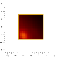
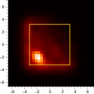
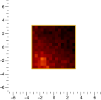
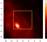
A single wavelength version of fig.1 is shown in fig.2, for $\lambda=3654$Å. The leftmost plot, which displays the data slice, shows that at this wavelength the signal to noise is very weak, as is the case for all wavelengths slices below the Balmer Break. Nevertheless, the comparison between the galaxy reconstruction and the ground truth show that for this slice the structure of the galaxy inside of the field is well reproduced. The field extrapolation also catches the large upper left galactic arm, and to some extent the lower right one. We observe that as expected the extension of the field extrapolation is similar to the PSF FWHM of $\sim 2.7$ spaxels or $\sim 1.1^{\prime\prime}$.

Figure 2: From left to right: data, reconstruction and ground truth for one single wavelength bin ($\lambda=3654$Å). The color bar is the same for all 3 figures, and is in relative units between the minimum and the maximum of the ground truth signal image. The golden box in the reconstruction and the ground truth images represent the data support region.

On the spectral side, Figure 3 displays the spectrum of the brightest galaxy spaxel for the ground truth in red and for the reconstruction in black. As stated above, we see that the galactic flux below 4000 Å is much lower than above. Nevertheless the galactic spectrum is well reconstructed at all wavelengths. The lower panel of the plot shows a zoom into the Ca H&K strong features that are reproduced with minimal bias. The spectrum of the data, displayed in dotted blue in both panels, illustrates the fact that the regularization only biases the spectrum reconstruction within the noise limits. For example the absorption trough at $\sim 4300$Å, larger than the Ca H&K lines in the lower panel of the figure, is reconstructed without bias.

Figure 3: Spectrum of the brightest spaxel of the reconstruction in black, superimposed over the same spaxel of the ground truth in red. Bottom plot is a zoom of the top plot on the region with largest spectral structure. In order to give a sense of the noise level of each spectra, we display in dotted blue the spectrum of the simulated data corresponding to the same location. Note also that in order to probe the quality of the relative reconstruction, and in order to remove the absolute differences due to variations of effective spatial resolution between the data, the truth and the reconstruction, we normalize all the spectra to the same average value

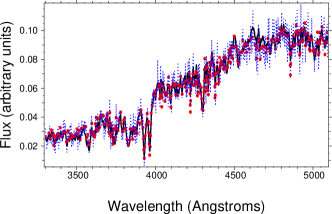
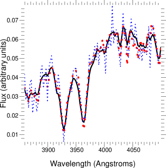
It has to be noted that if the spectral regularization slightly biases the reconstructed spectrum, it also allows for a consistent and effective reconstruction of the galaxy over the full wavelength range. Without such a regularization, each wavelength slice would be considered independently, and the noise level visible in the leftmost panel of Figure 2 would make it impossible to reconstruct the galaxy with the accuracy displayed in the middle panel of the same figure. The comparative gain of spectral regularization and spectral flattening will be addressed in more details in the next subsection (sec.6.3).

Figure 4: Residual maps of the galaxy reconstruction over 12 consecutive wavelength slices (spectral integrals on $\sim 150$Å wavelength bins). The residuals are normalized by the noise standard deviation on each pixel, giving a 2D vision of the histograms displayed in Figure 5

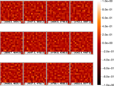
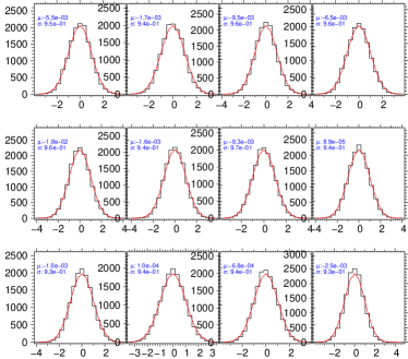
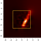
Figure 4 presents the residual map comparing the data and the model obtained once the reconstruction achieved. Its twelve thumbnails integrate the residual over $\sim 150$Å each ($\sim 50$ wavelength bins), and the residuals are normalized by the error. Figure 5 shows the histogram of these residuals normalized by the error (also called pull distribution). The mean values of the histograms, that measure the reconstruction bias, are below the 1% level for all but the slice including the two deep Ca H&K lines. For this later slice, the depth of the Ca H&K lines results in several wavelength bins with very low signal to noise. Because we don’t include the sky in this simulation, the absolute level of the signal in the Ca H&K trough is very small, leading to a small absolute value of the variance. In turn, this small value of the variance used to normalize the residual, results in a relatively large bias, even though its absolute value is very small. The RMS values, close to 1, show that the residuals are compatible with Gaussian noise. The systematic offset of 5%, between the RMS values observed and 1 tends to diagnose a slight over-fitting during the reconstruction process. This in turn will lead to some noise to be included in the reconstruction. Nevertheless the other results displayed previously show that this does not impact visibly on the quality of the reconstruction. In practice, it means that reaching minimal bias and an RMS within few percents of 1 is a good convergence criterion for trial and error estimation of the hyper-parameters.

Figure 5: Pull distribution of the residual slices displayed in fig.2. For each slice a Gauss curve of mean 0 and $\sigma=1$ is plotted in red. The mean and standard deviation of the distribution of each slice are reported in blue.

6.3 Comparison between regularization schemes

Figure 6 illustrates the relative impact of the regularizations. The left panel displays one wavelength slice of the reconstruction obtained with spectral and spatial regularization including spectral flattening, while the central panel displays the reconstruction obtained without spectral regularization, but still with spatial regularization including the spectral flattening. These plots show the same wavelength slice than Figure 2, i.e. $\lambda=3654$Å. The reconstruction without spectral regularization shows clear over fitting of the noise, apparent in the granularity of low galactic signal regions. The $\Delta\textrm{PSNR}$ of the reconstruction with both spectral and spatial regularization including spectral flattening is 5.2 dB, to compare to 0.1 dB for the reconstruction without spectral regularization.

The third plot from the left of Figure 6 displays the reconstruction obtained with both spatial and spectral regularizations but without spectral flattening. It shows a slight over fitting of the low signal regions of the galaxy compared to our best regularization, and yields a $\Delta\textrm{PSNR}$ of 4.1 dB. The rightmost panel of Figure 6 contains the true galaxy for comparison purposes.

Figure 6: From left to right: reconstruction with our better regularization, reconstruction without any spectral regularization and reconstruction with spectral regularization but with constant spatial and spectral hyper-parameters. The three images are displayed for one single wavelength bin ($\lambda=3654$Å). The color bar is the same for all 3 figures, and is in relative units between the minimum and the maximum of the ground truth signal image displayed in figure 2. The yellow box represents the data support region.

Figure 7: Spectrum of the brightest spaxel of the reconstruction in black, superimposed over the same spaxel of the ground truth in red. We display in green the spectrum of the reconstruction obtained without spectral regularization, and in dashed dark green the spectrum of the reconstruction obtained with spatial and spectral regularization but without spectral flattening. In order to probe the quality of the relative reconstruction, and in order to remove the absolute differences due to the difference of effective resolution between the data, the truth and the reconstruction, we normalize all the spectra to the same average value

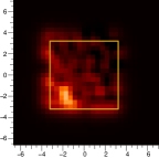
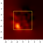
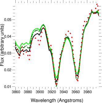
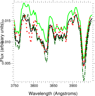
Figure 7 displays the spectra of the brightest spaxel of the reconstruction for all these three reconstruction cases plus the ground truth, zoomed on the same wavelength region than for Figure 3 bottom plot. The black curve, corresponding to our best regularization scheme is the closest to the ground truth, displayed in dotted red. The plain green curve, corresponding to the reconstruction obtained without spectral regularization, shows a consistent offset to the true spectrum: because of the lack of spectral regularization, the fit converges toward a solution that minimizes the spatial differences between the data and the model, to the detriment of the spectral reconstruction accuracy. The dashed dark green curve in turn corresponds to the reconstruction obtained without spectral flattening of the regularizations. Even though the regularization including spectral flattening does yield a more accurate reconstruction below 3910 Å, the gain is maybe less striking than in the spatial reconstruction. Figure 8 on the other hand illustrates better the gain of the procedure we propose, by showing the reconstruction accuracy of a spaxel directly outside of the field of view. The same colors are used for the different reconstructions, and the spaxel considered is the first spaxel outside of the field to the left (i.e along the $Ox$ axis) of the brightest galaxy spaxel in the reconstruction. In this case, the gain of the spectral flattening becomes more obvious: its ability to regularize more strongly the regions with low signal allows for a more accurate reconstruction of the spectral troughs.

Figure 8: Spectra of the first spaxel outside of the field of view, moving leftwards from the brightest spaxel of the reconstruction. The reconstruction using the full regularization scheme is displayed in black, superimposed over the same spaxel of the ground truth in red. We display in green the spectrum of the reconstruction obtained without spectral regularization, and in dashed dark green the spectrum of the reconstruction obtained with spatial and spectral regularization but without spectral flattening. In order to probe the quality of the relative reconstruction, and in order to remove the absolute differences due to the difference of effective resolution between the data, the truth and the reconstruction, we normalize all the spectra to the same average value

7 Results on real data

After checking the accuracy of the method on simulated data we examine the quality of the reconstruction on real data obtained with SNIFS. To that end we consider the host galaxy of the supernova SN2004gc discovered by The Lick Observatory Supernova Search and followed by the supernova factory. The exposure time of the final reference considered is 30 minutes. In order to probe the efficiency of the reconstruction of emission lines, we concentrate on the red channel, containing $\sim 1300$ wavelength bins and including H$\alpha$. The time needed for the reconstruction is $\sim 10$ minutes on a 2.4 GHz cpu.

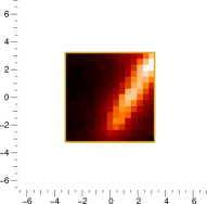
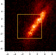
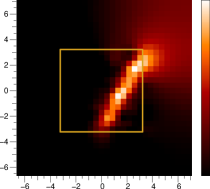
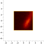
We display on the leftmost panel of Figure 9 the final reference datacube integrated over a synthetic top-hat V filter (with a throughput of 1 between 5200 and 6289 Å). The reconstruction is displayed on the middle panel, with a golden box materializing the spectrograph field of view. On the rightmost panel we display the stack of all V band acquisition images obtained by SNIFS photometric channel prior to each spectroscopic observation. This deeper image is on a slightly finer scale (pixel size: $0.28^{\prime\prime}\times 0.28^{\prime\prime}$) and observed through a V filter. In this plot also the golden box materializes SNIFS spectroscopic field of view. Comparison of the reconstruction with the acquisition image shows that the fine structure of the galaxy inside of the field is well reconstructed. Moreover the field extrapolation of both the bright core on the top right and the fainter arm on the center left of the top end of the field of view are well extrapolated.

Figure 9: SN2004gc host galaxy. The left plot displays the original data, the central one the stack of all acquisition images obtained by SNIFS imaging CCD prior to each spectral exposure, and the right plot displays the reconstructed galaxy. Both the original data and the reconstructed galaxy are integrated over a top-hat synthetic V filter. Each acquisition image is obtained through a $V$ filter, with a 2x2 binning, yielding a pixel size of $\sim 0.3^{\prime\prime}\times 0.3^{\prime\prime}$. The figure axis are labeled in arcseconds

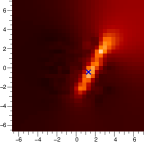
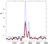
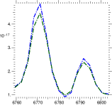
In figure 10 the same data and reconstruction are plotted on the two leftmost panels, this time integrated over $\sim 300$Å. The red cross corresponds to the position of the spectrum plotted in the third panel from the left. The spectrum of the data is displayed in black, the spectrum of the model in dotted red and the spectrum of the reconstruction in dotted blue. The bright region of the galaxy located under the red cross is spatially more localized in the reconstruction, showing the effects of the spatial deconvolution. At the same time, the flux in the data and the model at the location of the cross are in total agreement. The strong peaked lines displayed are enhanced by the reconstruction due to the spatial deconvolution. The presence of larger spectral variations in the reconstruction than in the data supports the claim that the spectral regularization we use does not induce any pathological over smoothing in the spectral direction. Moreover, the rightmost spectrum shows the comparative benefits of the regularization with spectral flattening compared to that without. The advantage of the former becomes obvious in this plot, as it yields a better reconstruction of these strong narrow lines.

Figure 10: The two first figures from the left represent respectively the data and the reconstruction integrated between 6600 Å and 6900 Å. The next figure displays the data spectrum in black, the model in dashed red, and the reconstruction spectrum in dotted blue over the same wavelength range for the location marked by a red cross in the two first figures. Finally, the rightmost spectra show in dotted blue the same reconstruction than in the previous plot, while the dotted green spectrum corresponds to the reconstruction without spectral regularization and the dashed dark green one corresponds to the reconstruction with spatial and spectral regularization but without spectral flattening

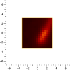
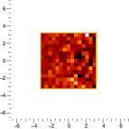
The leftmost panel of Figure 11 displays only one wavelength bin of the data, but this time corresponding to an other final reference than the one used for the reconstruction. This second final reference has been observed at a different epoch, with different seeing and different airmass. The reconstruction slice corresponding to the same wavelength is displayed on the second panel from the left. The next panel displays the model of the data obtained by reconvolution of the reconstruction by the PSF corresponding to the new exposure, and fitting of an additional flat background. The last panel to the right shows the residual of the subtraction of this model to the data displayed in the first panel. The wavelength selected for this slice corresponds to the maximum of the H$\alpha$ line displayed in the rightmost panel of Figure 10.

The residual shown at the right of Figure 11 is mainly flat. Results discussed in the next section will support the claim that these residuals are negligible with respect to the initial galactic flux. The absence of spatially structured residual concentrated at the top right corner of the residual image shows that the galactic light injected in the field of view by the PSF of this observation of the host galaxy of SN2004gc is well accounted for by the field extrapolation of our reconstruction. Moreover, the absence of structured residual in the rightmost plot of Figure 11 confirms that the reconstruction bias of strong peaked features is negligible: If that was not the case, the bright H$\alpha$ region visible at the center right of the reconstruction slice would cause a strong localized residual for an exposure observed under different conditions.

Figure 11: The leftmost panel displays a single wavelength bin of a data cube of the same host galaxy obtained at a different date, and under different conditions than the data used for the reconstruction. The second panel from the left displays the reconstruction in the same wavelength bin, corresponding to the strong H$\alpha$ emission line shown in Figure 10. Third and fourth to the right come the model of the data obtained with this reconstruction and the residual corresponding to the subtraction of this model from the data.

8 Discussion

The method we have presented shows both good spectral and spatial accuracy in the reconstruction of the 3-D image considered, both on simulated and real data. Even though the quality of the reconstruction on real data can not been checked against the ground truth, we propose here to discuss in more details the quality of the reconstruction of SN2004gc host galaxy 3-D cube.

The reason why we selected SN2004gc as study case is because 10 different final references have been observed over epochs spanning a large range of different observational conditions. This allows to select one final reference for the reconstruction and to use the 9 remaining final references to test the quality of the model obtained after reconstruction, accounting correctly for ADR. Table 1 shows in three synthetic top hat filters the flux of the data and of the residual integrated spatially over all spaxels and averaged over the 9 final references not used for the reconstruction. For convenience, it also shows in the fifth and sixth rows the relative value of the residual compared to the data for each of these synthetic filters. Based on those numbers, we see that the galactic reconstruction allows for a subtraction leaving much less than 1% of the initial flux in each spectral band. We checked that the error in color was completely negligible in both V-R, R-I and V-I. Note that the data rms is larger than the residual average because it is dominated by the sky variation from epoch to epoch, not by photon noise. Given that the final references used for this comparison have been observed under a range of observational conditions, table 1 shows that the galactic reconstruction, allows to account correctly and with negligible bias for the galactic signal in the field of view of SNIFS. Moreover, since the pointing variation between these exposures has an RMS of $\sim 0.5$ spaxels, the field extrapolation can be considered to have been tested under realistic assumptions.

Table 1: Results of the subtraction of the reconvolution of the reconstructed galaxy to 9 different other final references of SN2004gc host obtained under a large variety of observational conditions. All three filters are top hat filters with bandpasses $[$5200Å, 6289Å$]$ for V, $[$6289Å, 7607Å$]$ for R, $[$7607Å, 9200Å$]$ for I.

	V filter	R filter	I filter
Data	$9.3\,10^{{-13}}$	$1.2\,10^{{-12}}$	$1.9\,10^{{-12}}$
average
Data	$3.8\,10^{{-14}}$	$6.9\,10^{{-14}}$	$2.2\,10^{{-13}}$
RMS
Residual	$2.4\,10^{{-15}}$	$-1.9\,10^{{-15}}$	$-4.4\,10^{{-15}}$
average
Residual	$8.3\,10^{{-15}}$	$2.3\,10^{{-15}}$	$3.4\,10^{{-15}}$
RMS
Residual	0.3%	-0.2%	-0.2%
relat. avg
Residual	0.9%	0.2%	0.2%
relat. RMS

Figure 12: The three locations used to estimate the quality of the subtraction as shown in tables 2 and 3. The red cross corresponds to Position 1, the blue cross to Position 2, and the green cross to Position 3.

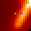
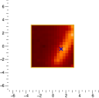
Since for a fixed PSF the extraction of a point source flux plus a flat background is a linear fit problem, it is easy to estimate the bias that an additional structured background would cause. Using the 9 final references not used for the 3-D image reconstruction allows to estimate this bias for a set of supernova positions in the field. The three locations selected, and shown in Figure 12, are the true location of SN2004gc (red cross), a bright region at the center of the host galaxy (blue cross), and a bright region on the edge of the microlens array (green cross). The average value of this bias as well as its rms for those three positions and two supernova apparent V magnitudes are shown in tables 2 and 3 under the denomination “Before”. The two magnitudes considered are $m_{V}=18.$ and $m_{V}=19.5$ in order to probe the typical dynamic scale of SNfactory supernovae.

Using the final reference reconstruction, we compute a galactic background model and subtract it to each one of the 9 additional final references considered. Using the residuals obtained, we then estimate the residual bias that this procedure would yield if it was to be used for host galaxy subtraction. The average and rms values of this bias are reported in tables 2 and 3 under the denomination “After”.

For the brighter case the bias after subtraction is well below the 1% level for the three synthetic filters considered, and for all three of the positions considered. The consistence of this bias value with zero for three positions with such a different host galactic pollution support the claim that the residual after subtraction is flat. The galactic reconstruction correctly accounts for all the spatial structure inside of the field of view, and extrapolates correctly the flux injected from outside of the field of view by the PSF, for a large variety of observational conditions. This claim is reinforced by the similar results of table 3, obtained for a much fainter supernova. The bias measured is below the 1% level on average and consistent with zero according to the error bars.

Table 2: Estimation of the bias on 9 different final references, before and after galactic subtraction in percentage of the SN flux for $m_{V,SN}=18.$. This corresponds to the apparent magnitude of SN2004gc 15 days after maximum light.

	V filter	R filter	I filter
Position 1
Before	44.6% $\pm$ 13.0%	49.8% $\pm$ 13.8%	45.7% $\pm$ 14.3%
After	-0.7% $\pm$ 0.5%	-0.2% $\pm$ 0.2%	-0.1% $\pm$ 0.2%
Position 2
Before	69.8% $\pm$ 15.7%	80.8% $\pm$ 18.0%	67.8% $\pm$ 17.6%
After	0.2% $\pm$ 0.9%	-0.2% $\pm$ 0.7%	0.3% $\pm$ 0.3%
Position 3
Before	61.4% $\pm$ 11.8%	74.1% $\pm$ 15.9%	67.7% $\pm$ 17.2%
After	0.4% $\pm$ 0.8%	0.0% $\pm$ 0.5%	1.3% $\pm$ 1.0%

Table 3: Estimation of the bias on 9 different final references, before and after galactic subtraction in percentage of the SN flux for $m_{V,SN}=19.5$. This is 0.5 magnitudes fainter than the apparent $V$ magnitude of SN2004gc 40 days after maximum light.

	V filter	R filter	I filter
Position 1
Before	177.5% $\pm$ 51.9%	198.4% $\pm$ 55.2%	181.8% $\pm$ 56.9%
After	-2.7% $\pm$ 2.0%	-0.0% $\pm$ 1.0%	-0.3% $\pm$ 0.8%
Position 2
Before	277.7% $\pm$ 62.4%	321.7% $\pm$ 71.7%	270.% $\pm$ 70.2%
After	0.9% $\pm$ 3.6%	-0.7% $\pm$ 2.9%	1.2% $\pm$ 1.3%
Position 3
Before	244.5% $\pm$ 47.0%	294.9% $\pm$ 63.4%	269.5% $\pm$ 68.5%
After	1.8% $\pm$ 3.4%	0.2% $\pm$ 2.0%	5.4% $\pm$ 3.9%

It is also to be noted that the algorithm we propose here trivially allows to calculate the galactic reconstruction using all the final references available simultaneously. Moreover, extending our approach to adjusting simultaneously all supernova exposures, even those including a supernova, opens exciting prospectives along the lines of the demixing of the supernova signal from the other components. Even though explorations we lead in this direction have yielded encouraging results, they are beyond the scope of the current paper.

Applying our algorithm to real data, we notice that the two hyper-parameters that our procedure leaves to tune are approximately the same for a range of SuperNova factory final references, with the default values $\mu_{\mathsf{spatial}}=10^{-3}$ and $\mu_{\mathsf{spectral}}=5\,10^{-3}$. This is not too surprising since the spectral variability is accounted for in the way we deal with the hyper-parameters. Also, in the redshift range considered, lots of the strong galaxies we have been concentrating on have similar spatial structures. On the other hand, more precise reconstruction can be achieved by refining the hyper-parameter values by trial and error. Further studies are needed to investigate the possibility of refining those values automatically: we still have to determine whether existing hyper-parameters setting methods (like SURE(Stein, 1981)) could be used or whether a more specific method has to be developed.

Another path of further studies worth mentioning concerns our use of quadratic regularization. In this work, we choose to enforce both spatial and spectral priors using quadratic regularization functionals in order to be able to estimate a posteriori covariance. However if scientific goals do not require such posterior covariance, a possibly better reconstruction could be achieved using non-quadratic regularization such as the edge preserving multispectral regularization proposed by Schultz & Stevenson (1995) or the total variation for vector-valued images (Sapiro & Ringach, 1996; Blomgren & Chan, 1998; Tschumperle & Deriche, 2002). These paths are currently under study.

9 Conclusion

We have seen that using the regularization scheme presented in Section 3.2 allows us to take advantage of the continuities present in the data. The reconstructions obtained allow for realistic field extrapolation and spectral reconstruction even of strong narrow lines. The field extrapolation, as well as the quality of the reconstruction inside of the field, even in spectral bins where the galactic signal is low, permit an accurate subtraction of the host galaxy of supernova observed by the SuperNova Factory. For typical SuperNova factory supernovae magnitudes, the subtraction residuals are below the percent level for all the synthetic filters considered. Given that this result is obtained on a set of final references intentionally obtained under very different observational conditions, this validates the quality of the reconstruction on real data.

Moreover, we have shown that the sharp galactic features are minimally biased in the reconstruction process both on simulations and real data. Even though the spatial and spectral regularization tend to bias the signal toward a smooth reconstruction, our use of spectrally variable hyper-parameters allows to maintain this bias below the noise level for all locations and wavelengths.

Our algorithm and the VMLM-B minimizer that we use can deal with the large number of parameters and data points needed to simultaneously adjust all final references obtained at once. Further work will expand in the direction of simultaneous demixing of the supernova signal: Encouraging results have been obtained by fitting simultaneously all exposures, including those containing the supernova. Another path worth exploring is that of the blind deconvolution. Given the strong smoothness of the wavelength dependence of the PSF, each exposure containing a supernova will yield strong constraints on the PSF shape, and could allow for a simultaneous adjustment of the PSF, demixing of the supernova signal from the others, and reconstruction of the host galaxy.

Even though changes in the data format and presentation could need non trivial implementation adjustments, the algorithm and method presented here translate directly to any data that has multiple instances of the same object in different spectral bands. As a consequence, this technique would be suitable for other projects that aim at obtaining hyper-spectral data in the future. MUSE for example (et al., 2003) will obtain images of $1^{\prime}\times 1^{\prime}$ regions of the sky from 480nm to 930nm with a spectral resolution of $3000$. This is typically a situation in which the techniques developed here could be applied. For example, even though the final goal of the technique we present is unbiased host subtraction, the image restoration method could also yield an increase in spectral and spatial resolution of the reconstructed image. This ability would be of special interests for weak lensing surveys, for which the measurement of the shape of the galaxy uncontaminated by the observational blur is of critical importance.

References

- Akgun et al. (2005) Akgun T., Altunbasak Y., Mersereau R., 2005, IEEE Trans. Image Process., 14, 1860
- Bacon (1995) Bacon e. a., 1995, Astronomy and Astrophysics Supplement Series, 113, 347
- Benazza-Benyahia & Pesquet (2006) Benazza-Benyahia A., Pesquet J.-C., 2006, in EUSIPCO Multichannel image deconvolution in the wavelet transform domain
- Bertero & Boccacci (1998) Bertero M., Boccacci P., 1998, Introduction to Inverse Problems in Imaging. Taylor & Francis
- Blomgren & Chan (1998) Blomgren P., Chan T. F., 1998, IEEE Trans. Image Process., 7, 304
- Bobin et al. (2009) Bobin J., Moudden Y., Starck J. L., Fadili J., 2009, in SPIE Conference Series Vol. 7446, Sparsity constraints for hyperspectral data analysis: linear mixture model and beyond. p. 42
- Bruzual & Charlot (2003) Bruzual G., Charlot S., 2003, Monthly Notices of the Royal Astronomical Society, 344, 1000
- Courbin et al. (2000) Courbin F., Magain P., Kirkove M., Sohy S., 2000, The Astrophysical Journal, 529, 1136
- Duijster et al. (2009) Duijster A., Scheunders P., Backer S. D., 2009, IEEE Trans. Geosci. Remote Sens., 47, 3892
- et al. (2003) et al. H., 2003, in Proceedings of SPIE Vol. 4841, MUSE, a second-generation integral-field spectrograph for the VLT. pp 1096–1107
- Frei et al. (1996) Frei Z., Guhathakurta P., Gunn J. E., Tyson J. A., 1996, The Astronomical Journal, 111, 174
- G. Aldering & et al. (2002) G. Aldering G., et al. 2002, in Tyson J. A., Wolff S., eds, Survey and Other Telescope Technologies and Discoveries Vol. 4836 of SPIE Conference, Overview of the nearby supernova factory. pp 61–72
- Galatsanos & Chin (1989) Galatsanos N., Chin R., 1989, IEEE Trans. Acoust., Speech, Signal Process., 37, 415
- Galatsanos et al. (1991) Galatsanos N., Katsaggelos A., Chin R., Hillery A., 1991, IEEE Trans. Signal Process., 39, 2222
- Gaucel et al. (2006) Gaucel J. M., Guillaume M., Bourennane S., 2006, in EUSIPCO Adaptive 3D-Wiener for hyperspectral image restoration: influence on detection strategy
- Hardie et al. (2004) Hardie R. C., Member S., Eismann M. T., Wilson G. L., 2004, IEEE Trans. Image Process., 13, 1174
- Hunt & Kubler (1984) Hunt B. R., Kubler O., 1984, IEEE Trans. Acoust., Speech, Signal Process., 32, 592
- Katsaggelos et al. (1993) Katsaggelos A., Lay K., Galatsanos N., 1993, IEEE Trans. Image Process., 2, 417
- Lucy & Walsh (2003) Lucy L. B., Walsh J. R., 2003, The Astronomical Journal, 125, 2266
- Molina et al. (2007) Molina R., Mateos J., Vega M., Katsaggelos A. K., 2007, in EUSIPCO Super resolution of multispectral images using locally adaptive models
- Mugnier et al. (2004) Mugnier L., Fusco T., Conan J.-M., 2004, J. Opt. Soc. Am. A, 21, 1841
- Neelamani et al. (2004) Neelamani R., Choi H., Baraniuk R., 2004, IEEE Trans. Signal Process., 52, 418
- Nocedal & Wright (1999) Nocedal J., Wright S., 1999, Numerical optimization. Springer
- Rodet et al. (2008) Rodet T., Orieux F., Giovannelli J.-F., Abergel A., 2008, IEEE J. Sel. Topics Signal Process., 2, 802
- Sapiro & Ringach (1996) Sapiro G., Ringach D. L., 1996, IEEE Trans. Image Process., 5, 1582
- Schultz & Stevenson (1995) Schultz R. R., Stevenson R. L., 1995, IEEE Trans. Image Process., 4, 1109
- Schulz (1993) Schulz T. J., 1993, JOSA-A, 10, 1064
- Sroubek & Flusser (2006) Sroubek F., Flusser J., 2006, Pattern Recognition Letters, 27, 287
- Stein (1981) Stein C., 1981, The Annals of Statistics, 9, 1135
- Tekalp & Pavlovic (1990) Tekalp M., Pavlovic G., 1990, Signal Processing, 19, 221
- Thiébaut (2002) Thiébaut E., 2002, in Starck J.-L., ed., Astronomical Data Analysis II. Vol. 4847, Optimization issues in blind deconvolution algorithms. pp 174–183
- Thévenaz et al. (2000) Thévenaz P., Blu T., Unser M., 2000, IEEE Transactions on Medical Imaging, 19, 739
- Tschumperle & Deriche (2002) Tschumperle D., Deriche R., 2002, IEEE Signal Process. Mag., 19, 16
- Vega et al. (2009) Vega M., Mateos J., Molina R., Katsaggelos A. K., 2009, The Computer Journal, 52, 153
- Vega et al. (2010) Vega M., Mateos J., Molina R., Katsaggelos A. K., 2010, Journal of Signal Processing Systems