Towards Completely Lifted Search-based Probabilistic Inference

Abstract

The promise of lifted probabilistic inference is to carry out probabilistic inference in a relational probabilistic model without needing to reason about each individual separately (grounding out the representation) by treating the undistinguished individuals as a block. Current exact methods still need to ground out in some cases, typically because the representation of the intermediate results is not closed under the lifted operations. We set out to answer the question as to whether there is some fundamental reason why lifted algorithms would need to ground out undifferentiated individuals. We have two main results: (1) We completely characterize the cases where grounding is polynomial in a population size, and show how we can do lifted inference in time polynomial in the logarithm of the population size for these cases. (2) For the case of no-argument and single-argument parametrized random variables where the grounding is not polynomial in a population size, we present lifted inference which is polynomial in the population size whereas grounding is exponential. Neither of these cases requires reasoning separately about the individuals that are not explicitly mentioned.

1 Introduction

The problem of lifted probabilistic inference in its general form was first explicitly proposed by Poole [2003], who formulated the problem in terms of parametrized random variables, introduced the use of splitting to complement unification, the parfactor representation of intermediate results, and an algorithm for multiplying factors in a lifted manner. de Salvo Braz et al. [2005; 2007] invented counting elimination for some cases where grounding would create a factor with size exponential in the number of individuals, but lifted inference can be done by counting the number of individuals with each assignment of values. Milch et al. [2008] proposed counting formulae as a representation of the intermediate result of counting, which allowed for more cases where counting was applicable. However, this body of research has not fulfilled the promise of lifted inference, as the algorithms still need to ground in some cases. The main problem is that the proposals are based on variable elimination [Zhang and Poole, 1994]. This is a dynamic programming approach which requires a representation of the intermediate results, and the current representations for such results are not closed under all of the operations used for inference. We sought to investigate whether there were fundamental reasons why we need to ground in some cases.

An alternative to variable elimination is to used search-based methods based on conditioning such as recursive conditioning [Darwiche, 2001] and other methods [see e.g., Bacchus et al., 2009]. The advantage of these methods is that conditioning simplifies the representations, rather than complicating them. The use of lifted search-based inference was proposed by Gogate and Domingos [2010], however to be both correct and able to do inference without grounding requires more attention to detail than given in that paper. This paper answer different questions than Jha et al. [2010].

Note that this paper is about exact inference. Lifted algorithms based on belief propagation (e.g. by Singla and Domingos [2008] and Kersting et al. [2009]) explicitly ignore the interdependence amongst the instances that exact inference needs to take into account.

In deriving an algorithm that never needs to ground, it is often the examples that demonstrate why simpler methods do not work that are most insightful. We have thus chosen to write this paper by presenting examples that exemplify the cases that need to be considered.

2 Background

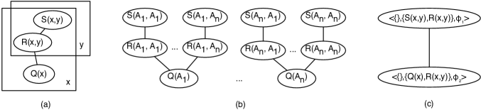
Figure 1: (a) a parametrized graphical model, (b) its grounding and (c) its parfactor graph

The problem of lifted inference arises in relational probabilistic models where there are probability distributions over random variables that represent relations which depend on individuals. Poole [2003] gives an example where the probability that a person fitting a description committed a crime depends on the population size, as this determines how many other people fit the description. We don’t want to reason about the other individuals separately. Rather, we would like to reason about them as a block considering only the number of such individuals.

A population is a set of individuals. A population corresponds to a domain in logic. The population size is the cardinality of the population which can be a finite number. For the examples below, where there is a single population, we write the population as $A_{1}\dots A_{n}$, where $n$ is the population size.

A parameter, which corresponds to a logical variable, is written in lower case. Parameters are typed with a population; if $x$ is a parameter of type $\tau$, $pop(x)$ is the population associated with $x$ and $|x|=|\tau|=|pop(x)|$. We assume that the populations are disjoint (and so the types are mutually exclusive). Constants are written starting with an upper case letter.

A parametrized random variable (PRV) is of the form $F(t_{1},\dots,t_{k})$ where $F$ is a k-ary functor (a function symbol or a predicate) and each $t_{i}$ is a parameter or a constant. Each functor has a range, which is $\{True,False\}$ for predicate symbols. A parametrized random variable represents a set of random variables, one for each assignment of an individual to a parameter. The range of the functor becomes the domain of the random variables.

A substitution is of the form $\{x_{1}/t_{1},\dots,x_{k}/t_{k}\}$ where $x_{i}$ are distinct parameters and $t_{i}$ are constants or parameters, such that $x_{i}$ and $t_{i}$ are of the same type. Given a PRV $r$ and a substitution $\theta=\{x_{1}/t_{1},\dots,x_{k}/t_{k}\}$, the application of $\theta$ on $r$, written $r\theta$ is the PRV with each $x_{i}$ replaced by $t_{i}$. A substitution $\theta=\{x_{1}/t_{1},\dots,x_{k}/t_{k}\}$ grounds parameters $x_{1}\dots x_{k}$ if $t_{1}\dots t_{k}$ are constants. A grounding substitution of $r$ is a substitution that grounds all of the parameters of $r$.

Probabilistic inference relies on knowing whether two random variables are the same. With parametrized random variables, we unify them to make them identical, but instead of just applying a substitution (as in regular theorem proving), Poole [2003] proposed to split parametrized random variables, forming the unifier and residual PRVs.

Example 1

Applying substitution $\{x/A,y/B\}$ to PRV $Foo(x,y,z)$ results in PRV that is the direct application, $Foo(A,B,z)$, and two “residual” PRVs, $Foo(x,y,z)$ with the constraint $x\neq A$ and $Foo(A,y,z)$ with the constraint $y\neq B$; these three parametrized random variables, with their associated constraints, represent the same set of random variables as $Foo(x,y,z)$.

A parametrized graphical model (Bayesian network or Markov network) is a network with parametrized random variables as nodes, and the instances of these share potentials. We need to be explicit about which instances share potentials.

Example 2

The parametrized graphical model of Figure 1 (a), is shown using parametrized random variables and plates (where the parameters correspond to plates). The plate representation represents $n$ instances of $Q(x)$ and $n^{2}$ instances of $R(x,y)$ in the grounding, shown in Figure 1 (b).

We assume the input to our algorithm is in the form of parfactors. A parametric factor or parfactor [Poole, 2003] is a triple $\langle C,V,\phi\rangle$ where $C$ is a set of inequality constraints on parameters, $V$ is a set of parametrized random variables and $\phi$ is a factor, which is a function from assignments of values to $V$ to the non-negative reals. $\phi$ is used as the potential for all instances of the parfactor that are consistent with the constraints. Milch et al. [2008] also explicitly include a set of parameters in their parfactors, but we do not. A parfactor means its grounding; the set of factors on $V\theta$ (all with table $\phi$) for each grounding substitution $\theta$ of $V$ that obeys the constraints in $C$.

2.1 Lifted Inference

Lifted variable elimination, such as in C-FOVE [Milch et al., 2008], allows for inference to work at the lifted level (doing unification and splitting at runtime or as a preprocessing step) like normal variable elimination, until we remove a PRV that contains the only instance of a free parameter or is linked to a PRV with a different set of parameters. At this stage, we need to take into account that the PRV represents a set of random variables.

Example 3

Suppose we have a factor on $S(x,y)$, $R(x,y)$ and $Q(x)$, as in Figure 1 (a). We can sum out all instances of $S(x,y)$, as all of the factors are the same, and get a new factor on $R(x,y)$; this does $n^{2}$ (identical) operations on the grounding in a single step. If we then remove $R$, we are multiplying a set of identical factors, and so can take their value to the power of the population size [Poole, 2003].

Suppose, instead, we were to first sum out $Q(x)$. In the grounding, for each individual $A_{i}$, the random variables $R(A_{i},A_{1})\dots R(A_{i},A_{n})$ are interdependent and so eliminating $Q$ results in a factor on $R(A_{i},A_{1})\dots R(A_{i},A_{n})$. The size of this factor is exponential in $n$.

de Salvo Braz et al. [2005] realized that the identity of the individuals is not important; only the number of individuals having each value of $R$. They introduced counting to solve cases such as removing $Q(x)$ first in polynomial time rather than the exponential time (and space) used for the ground case. They, however, do the counting and summing in one step, which limits its applicability. Milch et al. [2008] defined counting formulae that give a representation for the resulting lifted formula and can then be combined with other factors. This expanded the applicability of lifted inference, but it still requires grounding in some cases.

2.2 Search-based probabilistic inference

An alternative to lifting variable elimination is to lift a search-based method.

input: $Con$: a set of $variable=value$ assignments

$Fs$: set of factors

output: a number representing $\sum_{\overline{x}}\prod_{F\in Fs}F(\overline{x}|Con)$

if $vars(Con)\not\subseteq vars(Fs)$ then {Case 0}

       return $rc(\{(x=V)\in Con:x\in vars(Fs)\},Fs)$

if $\exists v$ such that $\langle\langle Con,Fs\rangle,v\rangle\in cache$ then {Case 1}

       return $v$

else if $\exists f\in Fs:vars(f)\subseteq vars(Con)$ then {Case 2}

       $F_{0}\leftarrow\{f\in Fs:vars(f)\subseteq vars(Con)\}$

       return $\left(\prod_{f\in F_{0}}eval(f,Con)\right)\times rc(Con,Fs\setminus F_{0})$

      

else if factor graph $\langle Con,Fs\rangle$ is disconnected then {Case 3}

       $\textnormal{{return}}\prod_{\mbox{connected component }cc}rc(Con,cc)$

else {Case 4}

       select variable $x\in vars(Fs)\setminus vars(Con)$

       $sum\leftarrow 0$

       for each value $v$ of $x$ do

             $sum\leftarrow sum+rc(\{x=v\}\cup Con,Fs)$

            

      $cache\leftarrow cache\cup\{\langle\langle Con,Fs\rangle,sum\rangle\}$

       return $sum$

      

Algorithm 1 Recursive Conditioning: $rc(Con,Fs)$

The classic search-based algorithm is recursive conditioning [Darwiche, 2001], a version of which is presented in Algorithm 1. This algorithm is presented in this non-traditional way, to emphasize the cases that need to be implemented for lifting. In particular, decoupling branching and the evaluation of factors is useful for developing its lifted counterpart. The correctness does not depend on the order of the cases (although efficiency does). In this algorithm $Con$ is a context, a set of $variable=value$ assignments, and $Fs$ is a set of input factors (this algorithm never creates or modifies factors; it only evaluate them when all of their variables are assigned). We separate the context from the factors; typically these are combined to give what could be called partially-assigned factors.

In case 0, if there are variables that appear in $Con$ that do not appear in $Fs$, these are removed from $Con$. This is called “forgetting” in the description below; we forget the context that is not relevant for the rest of the factors. $vars(S)$ is the set of variables that appear in $S$.

In case 1, the cache contains a set of previously computed values. If a value has already been computed it can be recalled. Initially the cache is $\{\left<\langle\{\},\{\}\rangle,1\right>\}$.

For case 2, if all of the variables that appear in a factor $f$ are assigned in $Con$, $eval(F,Con)$ returns the number that is the value of $F$ for the assignment $Con$. These numbers are multiplied.

For case 3, a factor graph on $\langle Con,Fs\rangle$ is a graph where the nodes are factors in $Fs$, and there is an arc between factors that share a random variable that isn’t assigned in $Con$. The connected components refer to the nodes that are connected in this graph. The connected components can be solved separately, and their return values multiplied.

Case 4 branches on a variable $x$ that isn’t assigned. The efficiency, but not the correctness, of the algorithm depends on which variable $x$ is selected to be branched on.

To compute $P(x|Obs)$, for each value $v$ of $x$, call $rc(\{x=v\}\cup Obs,Fs)$ where $Fs$ is the set of all factors of the model, and normalize the results.

An aspect that is important for lifted inference is that when values are assigned, the factors are simplified as they are now functions of fewer variables. This should be contrasted to variable elimination that constructs more complicated factors.

3 Search-based Lifted Inference

In this section, we develop a lifted search-based algorithm. We show its correctness with respect to a parallel ground algorithm that uses the same order for splitting. Note that, because the lifted algorithm removes multiple variables at once, this restricts the order the variables are split in the ground algorithm. A legal ordering for the lifted inference branches on all instances of a PRV at once, whereas the corresponding ground algorithm branches on all instances sequentially. We show how the complexity (as a function of the population size) of the lifted algorithm is reduced compared to the corresponding ground algorithm. Because we want our algorithm to be correct for all legal branching orderings, we ignore the selection of which variable to branch on; this can be optimized for efficiency.

We assume that we can count the number of solutions to a CSP with inequality constraints in time that is at most logarithmic in the domain size of the variables (e.g., by adapting the #VE algorithm of Dechter [2003] to not enumerate the undistinguished variables).

3.1 Intermediate Representations

The lifted analogy of a context in Algorithm 1 is a counting context which represents counts of assignments to parametrized random variables.

A counting context on $V$ is a pair $\langle V,\chi\rangle$, where $V$ is a set of PRVs (all taking a single argument of the same type), all parametrized by the same parameter, and $\chi$ is a table mapping assignments of PRVs in $V$ into non-negative integers. A counting context represents a context in the grounding. For each individual of the type, the table $\chi$ specifies how many of the individuals take on that tuple of values. We can also treat a counting context in terms of $\chi$ as a set of pairs of the assignment of values to $V$ and the corresponding count.

Example 4

A counting context for $V=\{R(x),T(x)\}$, and

$$\chi= \left\{\begin{array}[]{cc|c}R(x)&T(x)&Value\\ \hline\cr True&True&20\\ True&False&40\\ False&True&10\\ False&False&20\end{array}\right.$$

represents the assignment of values to $R$ and $T$ for $90$ ($20+40+10+20$) individuals. 20 of these have both $R(\dots)$ and $T(\dots)$ true, 40 have $R(\dots)$ true and $T(\dots)$ false, etc.

There is a separate counting context for each type. A current context is a set of pairs either of the form $\langle Var,Value\rangle$ where $Var$ is a PRV that has no parameters, or of the form $\langle\tau,CC\rangle$ where $\tau$ is a type and $CC$ is a counting context where the parameter of each of the PRVs in $CC$ is of type $\tau$. A current context can have at most one pair for each type.

A PRV $P$ is assigned in a current context $Con$ if it has no parameters and $\langle P,Val\rangle\in Con$, or if it is parametrized by a variable of type $\tau$ and if $\langle\tau,\langle V,\chi\rangle\rangle\in CC$ and $P$ unifies with an element of $V$.

A parfactor graph on $\langle Con,G\rangle$ where $Con$ is a current context and $G$ is a set of parfactors, has the elements of $G$ as nodes, and there is an arc between parfactors $\langle C_{1},V_{1},\phi_{1}\rangle$ and $\langle C_{2},V_{2},\phi_{2}\rangle$ if there is an element of $V_{1}$ that isn’t assigned in $Con$ that unifies with an element of $V_{2}$ such that the unifier does not violate any of the constraints in either parfactor.

The grounding of a parfactor graph on $\langle Con,G\rangle$ is a factor graph on $\langle Con^{\prime},G^{\prime}\rangle$, where for every counting parfactor $\langle S,F,\theta\rangle$ in $G$, and for every grounding substitution $\psi$ of all of the free parameters that does not violate $S$, $F\psi$ is in $G^{\prime}$ with table $\theta$. $Con^{\prime}$ represents all of the ground instances that are assigned in $Con$, with the corresponding counts given by the table in $Con$.

The grounding of a parfactor graph defines its semantics. We carry out lifted operations so that the lifted operations have the same result as carrying out recursive conditioning on the grounding of the parfactor graph for the same elimination ordering.

3.2 Symmetry and Exchangeability

The reason we can do lifted inference is because of symmetries. Having a symmetry between the unnamed individuals means that a derivation about some of the individuals can be equally applied to any of the other individuals.

We say that a set of individuals are exchangeable in a parfactor graph if the grounding of the parfactor graph with one consistent assignment of individuals to variables is isomorphic to the grounding of the graph with another assignment. Graph isomorphism means there is a 1-1 and onto mapping between the nodes where the factors are identical. Exchangeability means that reasoning with some of the individuals can be applied to the other individuals.

3.3 Unification, splitting and shattering

In order to determine which instances of parametrized random variables are the same random variables, Poole [2003] used unification and splitting on logical variables, which guarantees that the instances are identical or are disjoint. de Salvo Braz et al. [2005] proposed to do all of the splitting up-front in an operation called shattering (see Kisynski and Poole [2009] for analysis of splitting, shattering and related operations).

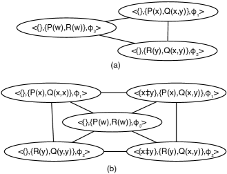
Figure 2: A parfactor graph that is problematic for shattering and its preemptively shattered counterpart

Shattering is a local operation and does not imply graphs constructed by substitutions are isomorphic as in the following example:

Example 5

Consider the network of Figure 2 (a). Although it is shattered, the instances with $x=y$ have a different grounding from the instances where $x\neq y$. This graph can be split, on $x=y$ in the right-hand parfactors, giving the network shown in Figure 2 (b).

An alternative to the local shattering is to carry out a more global preemptive shattering. A set of parfactors preemptive shattered if

• for every type, and every constant $C$ of the type that is explicitly mentioned, every parfactor that contains a variable $x$ of the type includes the constraint $x\neq C$.

• if variables $x$ and $y$ of the same type are in a parfactor, the parfactor contains the constraint $x\neq y$.

Given a set of parfactors, to construct an equivalent set of preemptively shattered set of parfactors, all logical variables in a parfactor are split with respect to all explicitly given constants, and any pairs of logical variables in a parfactor are split with respect to each other.

Preemptive shattering gives more splits than shattering, and sometimes more than needed, but it allows our proofs to work and does not prevent the asymptotic complexity results we seek. With preemptive shattering, counting the number of instances represented by a parfactor is straightforward; there are no complex interactions. For the rest of this paper, we assume that all parfactors are preemptively shattered.

Note that, as can be seen in the parfactor graph of Figure 2 (b), even after preemptive shattering, we cannot always globally rename variables so that the unifying variables are identical.

3.4 Disconnected Grounding

When the graph is disconnected, Algorithm 1 considers the connected components separately, and multiplies them. In this section, we cover all of the cases where the grounding is disconnected, and show how it corresponds to operations in the lifted case.

If the lifted network is disconnected, the ground counterpart is disconnected, and so these disconnected components can be solved separately and multiplied.

If the lifted network is connected, this does not imply that its grounding is connected. For example, the parfactor graph of Figure 1 (c) is connected yet its grounding is not connected.

Intuitively, if there is a logical variable that is in all of the counting parfactors, the instances for one individual are disconnected from the instances for another individual. Thus, we can the solve the problem for one of the individuals, and the value for the lifted case is that value to the power of the number of individuals.

This intuition needs to be refined because logical variables are local to a parfactor; renaming the variables gives exactly the same grounding. There are cases where chains of unifications cause connectedness:

Example 6

The parfactor graph

does not have disconnected ground instances, even though $x$ is in every PRV. For three individuals, $C_{1},C_{2},C_{3}$, in the grounding $R(C_{1},C_{3})$ is connected to $R(C_{2},C_{3})$ through $S(C_{3})$ in the grounding of the bottom parfactor, thus $S(C_{1})$ is connected to $S(C_{2})$ for any different $C_{1}$ and $C_{2}$, using the top parfactor.

This reasoning can be applied generally:

Suppose $x$ is a logical variable in parfactor $\langle C,V,\phi\rangle$ that appears in parfactor graph $G$. $connected(x,\langle C,V,\phi\rangle,Con,G)$ means the instances of $x$ in parfactor $\langle C,V,\phi\rangle$ are connected to each other in the grounding of $\langle Con,G\rangle$. $connected$ can be defined recursively as follows.

$connected(x,\langle C,V,\phi\rangle,Con,G)$ is true if and only if:

• $x$ appears in $V$, is not assigned in $Con$ and there is a PRV in $V$ that is not assigned in $Con$ and not parametrized by $x$ or

• there is a parfactor $\langle C^{\prime},V^{\prime},\phi^{\prime}\rangle$ in $G$, such that an element of $V$ unifies with an element of $V^{\prime}$ (in a manner consistent with $C$ and $C^{\prime}$, and that are not assigned in $Con$) and $x$ is unified with a variable $x^{\prime}$ such that $connected(x^{\prime},\langle C^{\prime},V^{\prime},\phi^{\prime}\rangle,Con,G)$ is true.

The definition of $connected$ is sound: if $connected(x,\langle C,V,\phi\rangle,Con,G)$ is true, the instances of $x$ are connected in the grounding. The proof for the soundness is a straightforward induction proof; essentially the algorithm is a constructive proof.

However, the definition is not complete: there can be instances that are connected even though $connected$ is false. It is instructive to see what a proof for completeness would look like. To prove completeness, we would prove that all instances of $x$ are disconnected if the above construction fails to derive they are connected. Suppose there are two constants $C$ and $C^{\prime}$, we need to show that the graph with $x$ replaced by $C$ is disconnected with the graph with $x$ replaced by $C^{\prime}$. The graph with $x$ replaced by $C$ has $C$ in every PRV (by construction) and the graph with $x$ replaced by $C^{\prime}$ has $C^{\prime}$ in every PRV. However, this does not imply that the graphs are disconnected as there could be a PRV that contains both $C$ and $C^{\prime}$, as in the following example:

Example 7

Consider the parfactor graph:

In the grounding, for all individuals $C_{i}\neq C_{j}$, the random variable $S(C_{i},C_{j})$ is connected to $S(C_{j},C_{i})$. However, it is disconnected from other instances of $S(x,y)$.

We use the definition of $connected$ to detect potentially disconnected components, and we can explicitly check for which instances are connected. In this way, we can ensure that the lifted algorithm detects disconnectedness whenever the ground algorithm would. The only counterexamples to the completeness of $connected$ are when there is a set of variables, all with the same domain, and all of them appear in all PRVs in the parfactor graph (possibly renamed), and there is an inequality constraint between them. Suppose there are $k$ such variables, $x_{1}\dots,x_{k}$, in a parfactor. We choose $k$ constants, $C_{1},\dots,C_{k}$, and apply the substitution $\{x_{1}/C_{1},\dots,x_{k}/C_{k}\}$ to that parfactor, and then proceed to ground out all the corresponding variables in the other factors by unifying with the factors in all ways, forming a generic connected component. We then need to count the number of copies of each PRV instance in the connected component; suppose this is $c$. For a population size of $n$, there are $n(n-1)\dots(n-k+1)$ instances of the PRV, and there are $c$ elements in each connected component, therefore there are $n(n-1)\dots(n-k+1)/c$ disconnected components. If we compute $p$ as the probability of the generic connected component, we need to take $p$ to the power $n!/((n-k)!\times c)$ to compute the probability of the lifted network.

In the above analysis, $n$ is the population size and $k$ and $c$ depend only on the structure of the graph, and not on the population size. As we assume that we can count the population size in time logarithmic in the population size, the above procedure is polynomial in the log of the population size, whereas grounding is polynomial in the population size. As we see below, this is the only case where the grounding is polynomial in the population size.

In Example 7, $k=2$ and $c=2$, and so the power is $n(n-1)/2$. In an example with $k=3$, it is possible that $c$ could be 1,2,3 or 6.

Algorithm 2 gives the lifted variant of case 3 of Algorithm 1. The main loop is the same as Algorithm 1, with the recursive call $lrc(Con,Fs)$ where $Con$ is a current context and $Fs$ is a set of counting parfactors.

if $Fs$ is disconnected then {Case 3a}

       $\textnormal{{return}}\prod_{\mbox{connected component }cc}lrc(Con,cc)$

else if $\exists x~{}\neg connected(x,F,Con,Fs)$ for $F\in Fs$ then {Case 3b}

       Select one $x$ such that $\neg connected(x,F,Con,Fs)$

       let $\tau$ be the type of $x$

       let $C=\{x\mbox{ of type }\tau:\neg connected(x,F,Con,Fs)\}\mbox{ for some }F\in Fs$

       let $k=|C|$

       replace $x_{1},\dots,x_{k}$ with $C_{1},\dots,C_{k}$ in $F$

       unify $F$ with all other factors in $Fs$

       let $c=|\{$instances of $F$ in $Fs\}|$

       let $e=n!/((n-k)!\times c)$

       return $lrc(Con,Fs)^{e}$

      

Algorithm 2 Lifted search, case 3: grounding is disconnected.

3.5 Counting

Once we have a single connected component (and there is no logical variable for which its instances are connected), we select a PRV to branch on. In describing this, as in Algorithm 1, we decouple branching on a variable, and evaluating parfactors. Typically a PRV is associated with many parfactors, and when we branch on a PRV we need to count the number of instances with various values for the PRV. We need to make sure that we branch in a way that enables us to evaluate the relavant parfactors.

For the simplest case, assume we want to sum out a Boolean PRV $F(x)$ that has one free logical variable, $x$, with domain $\{A_{1},\dots,A_{n}\}$. The idea behind counting [de Salvo Braz et al., 2007] is that only the number of exchangeable individuals that have a PRV having a particular value matters, not their identity. We present counting first considering this simple case, then more complex cases.

In counting branching, for each $i$, such that $0\leq i\leq n$, the algorithm generate the branch where there are $i$ instances of $F$ true, and so $n-i$ instances of $F$ false. This branch represents $\binom{n}{i}$ paths in the grounding, as there are this many renamings of constants that would result in the same assignment. Thus it can multiply the result of evaluating this branch by $\binom{n}{i}$. Note that the counting branching involves generating $n+1$ branches, whereas in the grounding there are $2^{n}$ assignments of values after the equivalent ground branching. The resulting counting context records the number of instances of $F$ that are true and number that are false.

We now show how to evaluate various cases of parfactors that can include $F$. The general case is a combination of these specific cases. For all of the example below, assume they are part of a larger parametrized graphical model. In particular, assume that the instances are connected, so that the case described in the previous section does not apply.

Example 8

Consider the parfactor

$$\langle\{\},\{F(x),E\},\phi_{1}\rangle$$

Suppose $|x|=n$. This parfactor represents $n$ factors. Suppose $\phi_{1}$ is:

$$\begin{array}[]{ll|l}F(x)&E&\phi_{1}\\ \hline\cr True&True&\alpha_{1}\\ True&False&\alpha_{2}\\ False&True&\alpha_{3}\\ False&False&\alpha_{4}\end{array}$$

Suppose we have split on $E$ and assigned it the value $True$,and then we split on $F(x)$ and are in the branch with $F=True$ for $i$ cases and $F=False$ for $n-i$ cases. This is represented by the current context:

$$E=true,\begin{array}[]{l|l}F(x)&\phi_{1}\\ \hline\cr True&i\\ False&n-i\\ \end{array}$$

The contribution of this parfactor in this current context is $\alpha_{1}^{i}\alpha_{3}^{n-i}$.

Example 9

Consider the parfactor

$$\langle\{\},\{F(x),G(y)\},\phi_{2}\rangle$$

Suppose $x$ and $y$ are of different types, where $|x|=n$, $|y|=m$. $\phi_{2}$ is:

$$\begin{array}[]{ll|l}F(x)&G(y)&\phi_{2}\\ \hline\cr True&True&\alpha_{1}\\ True&False&\alpha_{2}\\ False&True&\alpha_{3}\\ False&False&\alpha_{4}\end{array}$$

This parfactor represents $nm$ factors; for each combination of assignments of values to the instances of $F$ and $G$, there is a factor. In a current context with $i$ $F$’s true and $h$ $G$’s true, this parfactor has a contribution:

$$\alpha_{1}^{ih}\alpha_{2}^{i(m-h)}\alpha_{3}^{(n-i)h}\alpha_{4}^{(n-i)(m-h)}.$$

Example 10

Consider the parfactor

$$\langle\{\},\{F(x),G(x)\},\phi_{2}\rangle$$

Suppose $|x|=n$. This parfactor represents $n$ factors. Unlike the previous cases, counting branching is not adequate; we need to consider which $F$-assignments go with which $G$-assignments. We can do a counting branch on $F$ first: for each $i\in[0,n]$, consider the case where $F$ is true for $i$ individuals, and is false for $n-i$ individuals. This case represents $\binom{n}{i}$ branches in the grounding. To split on $G$ we can do a dependent branch: consider the $i$ individuals for which $F$ is true, and the $n-i$ individuals for which $F$ is false separately. For each $j\in[0,i]$, we consider the branch where $G$ is true for $j$ individuals and false for $i-j$ individuals all with $F=True$; this branch corresponds to $\binom{i}{j}$ ground branches. For each $k\in[0,n-i]$ we construct the branch where $G$ is true for $k$ individuals and is false for $i-j-k$ individuals with $F=False$. This represents $\binom{n-i}{k}$ ground cases. This branch is represented by the counting context:

$$\begin{array}[]{ll|l}F(x)&G(x)&\phi_{2}\\ \hline\cr True&True&j\\ True&False&i-j\\ False&True&k\\ False&False&n-i-k\end{array}$$

The contribution of the parfactor in this branch is:

$$\alpha_{1}^{j}\alpha_{2}^{i-j}\alpha_{3}^{k}\alpha_{4}^{n-i-k}$$

Example 11

Consider the parfactor

$$\langle\{x\neq y\},\{F(x),G(y)\},\phi_{2}\rangle$$

Suppose $x$ and $y$ are of the same type, where $|x|=|y|=n$. This parfactor represents $n(n-1)$ factors. This can be solved by a mix of the previous two examples. If we were to do the same as Example 9, we would also include the cases where $x=y$, which are explicitly excluded; but these are the cases in Example 10. So the contribution of this factor can be computed by dividing the result of Example 9 by the result of Example 10, or equivalently subtracting the exponents. As in Example 10, we consider the case where $F$ is true for $i$ individuals, and for these individuals $G$ is true for $j$ of them, and out of the individuals where $F$ is false, $G$ is true for $k$ of them. Taking the difference between the exponents Example 9 and 10, and noticing that $h$ in Example 9 corresponds to $j+k$ in Example 10, the contribution of these factors is:

$$\alpha_{1}^{i(j+k)-j}\alpha_{2}^{i(n-j-k)-i+j}\alpha_{3}^{(n-i)(j+k)-k}\alpha_{4}^{(n-i)(n-j-k)-n+i+k}$$

Example 12

Consider a mix between the previous examples. Suppose we have the parfactors:

$$\langle\{\dots\},\{F(x),G(x),\dots\}\rangle$$

$$\langle\{x\neq y,\dots\},\{H(y),G(x),\dots\}\rangle$$

where all of the variables are of the same type with $n$ individuals. Suppose the branching order is to branch on $H$, then $F$, then $G$. The split on $G$ needs to depend on both $H$ and $F$. This can be done if the splits on $H$ and $F$ are dependent; that is, we do a separate count on $F$ for the individuals for which $H$ are true and the individuals for which $H$ are false. Then we do a separate count on $G$ for the set of individuals for each combination of values to $H$ and $F$.

Counting branching needs to be expanded to cascaded counting branching. Dependent counting branching on a PRV $X$ that is parametrized by a parameter of type $\tau$, works as follows. First, we find the corresponding counting context $\langle V,\chi\rangle$ for $\tau$. Dependent Counting branching replaces this with a counting context on $\langle V\cup\{X\},\chi^{\prime}\rangle$ as follows. For each assignment $\langle t,i\rangle$ in the table $\chi$ ($i$ is the count for assignment $t$), for each $j$ in $[0,i]$, we create the table $\chi^{\prime}$ that maps $t\cup\{X=true\}$ to $i$ and $t\cup\{X=false\}$ to $i-j$. This assignment corresponds to $\binom{i}{j}$, different grounding assignments, so the grounding needs to be multiplied by $\binom{i}{j}$. This is recursively carried out for each tuple.

Example 13

Starting from the current context of Example 8, dependent counting branching on $G(x)$ produces the counting context of Example 10. This context corresponds to $\binom{i}{j}\binom{n-i}{k}$ contexts in the grounding. Note that there are $i(n-i)$ leaves that are decedents of the current context created in Example 8, whereas in the grounding there are $2^{n}$ leaves that are descendants of each corresponding ground context.

Branching is shown as Case 4 in Algorithm 3. In this algorithm $Con$ is a current context and $Fs$ is a set of input parfactors. Case 4a is the same as case 4 in Algorithm 1 (but for Boolean variables). Case 4b is for branching on a PRV with a single parameter, and sets up dependent counting branching that is presented in Algorithm 4. Note that this treats a counting context as a set of pairs of an assignment of values to a set of PRVs and a count (as described in Section 3.1).

The branching factor depends on the population, but the depth of the recursive calls depends on the structure of the counting context, and not on the population size. The depth of the recursive calls provides the power of the polynomial. If we use a sparse representation of current contexts with zeros suppressed, this is never worse than grounding. [However, whether we use a sparse or dense representation is something that can be optimized for.]

input: $Con$: current context

$Fs$: set of parfactors

output: a number representing $\sum_{\overline{x}}\prod_{F\in grounding(Fs,Con)}F(\overline{x})$

if $\exists x\in vars(Con)\setminus vars(Fs)$ then {Case 0}

       return $lrc(\sum_{X}Con,Fs)$

if $\exists v$ such that $\langle\langle Con,Fs\rangle,v\rangle\in cache$ then {Case 1}

       return $v$

else if $\exists f\in Fs:vars(f)\subseteq vars(Con)$ then {Case 2}

       return $eval\_parfactor(f,Con)\times lrc(Con,Fs\setminus\{f\})$

      

else {Case 3}

      See Algorithm 2

else {Case 4}

       select PRV $X\in vars(Fs)\setminus vars(Con)$

       if $X$ contains no parameters then {Case 4a}

             $sum\leftarrow lrc(\{X=true\}\cup Con,Fs)+lrc(\{X=false\}\cup Con,Fs)$

            

      else {Case 4b}

             suppose the parameter of $X$ is of type $\tau$

             if $\exists\chi:~{}\langle\tau,\chi\rangle\in Con$ then

                   $sum\leftarrow branch(\chi,X,\{\},Con\setminus\{\langle\tau,\chi\rangle\},Fs)$

                  

            else

                   $sum\leftarrow branch(\{\langle\langle\rangle,|\tau|\rangle\},X,\{\},Con,Fs)$

                  

      $cache\leftarrow cache\cup\{\langle\langle Con,Fs\rangle,sum\rangle\}$

       return $sum$

      

Algorithm 3 Lifted Recursive Conditioning: $lrc(Con,Fs)$

input: $\chi$: a set of tuples from a counting context

$X$: the PRV to branch on its instances

$\chi^{\prime}$: the new counting context being constructed

$Con$: the current context to be added to

$Fs$: the set of all factors

if $\chi=\{\}$ then

       Suppose $\tau$ is the type of the parameter in $V$

       return $lrc(Con\cup\{\langle\tau,\chi^{\prime}\rangle\},Fs)$

      

else

       select $\langle t,i\rangle\in\chi$

       $sum\leftarrow 0$

       for $j\in[0,i]$ do

             let $\chi^{\prime\prime}$ be $\chi^{\prime}\cup\langle t\cup\{X=true\},j\rangle\cup\langle t\cup\{X=false\},i-j\rangle$

             $sum\leftarrow sum+\binom{i}{j}branch(\chi\setminus\{\langle t,i\rangle\},\chi^{\prime\prime},Con,Fs)$

            

      return sum

      

$branch(\chi,X,\chi^{\prime},Con,Fs)$

Algorithm 4 Dependent Counting Branching:

$branch(\chi,X,\chi^{\prime},Con,Fs)$

The main remaining part of the lifted algorithm is to evaluate a parfactor $\langle C,V,\phi\rangle$ in a counting context $\langle V^{\prime},\chi\rangle$, where all of the variables in $V$ are assigned in $V^{\prime}$. There are three cases: shared parameters, different parameters of the same type and parameters of different types. One parfactor can contain all of these.

For shared parameters, as in Example 10, the parfactor provides the base, and there is a unique counting context that provides the powers. First we group all of these together and raise them to the appropriate powers, and then treat them as a block.

For parameters of different types, as in Example 9, we need to multiply the powers. We can treat the shared parameters as a block.

For different parameters of the same type, as in Example 11, we can use the other two cases: first we treat them as different types (which over-counts because it includes the equality cases), and then divide by the case when they are equal. We also have to readjust for double counting, which can be done using the coefficient of $n!/(n-k)!$ where $k$ is the number of such cases. For example, when $k=3$, this is $n(n-1)(n-2)=n^{3}-3n^{2}+2n$. The first of these corresponds to all parameters being different, the second to all pairs of parameters equal, and the third to all parameter the same.

Algorithm 5 shows how to evaluate a parfactor in a current context. It omits the last case, as it is computed from the other two cases.

input: $PF$: a parfactor

$Con$: a current context

Suppose $PF$ is $\langle C,V,\phi\rangle$

Suppose $Con$ is $\langle V^{\prime},\chi\rangle$

$prod\leftarrow 1$

foreach $\langle t,p\rangle\in\phi$ do

       if $t$ is consistent with variable assignments in $Con$ then

             $power\leftarrow 1$

             Let $\tau$ be the type of $X$

             Select $\langle\tau,\langle V^{\prime\prime},\chi\rangle\rangle\in Con$

             $RedundantVars\leftarrow vars(V^{\prime\prime})\setminus vars(V)$

             $power\leftarrow power\times\sum_{\langle t,i\rangle\in\chi:consistent(t,V)}i$

            

      $prod\leftarrow prod\times p^{power}$

return $prod$

$eval\_parfactor(PF,Con)$

Algorithm 5 Evaluating a parfactor in current context:

$eval\_parfactor(PF,Con)$

Example 12 (cont.)

Consider the branch where $H$ is true for $i$ individuals and false for $n-i$ individuals. Suppose we then branch on $F$. We then consider the branch with $F$ true for $j_{0}$ of the cases where $H$ is false and $j_{1}$ cases where $H$ is true. We thus have: $j_{1}$ individuals for which $F$ and $H$ are true; $i-j_{1}$ individuals which have $H$ true and $F$ false; $j_{0}$ individuals that have $H$ false and $F$ true; and $n-i-j_{0}$ individuals what have both $H$ and $F$ false. We can then branch on $G$, for each of the four sets of individuals. We thus know the counts of each case; Algorithm 5 computes the contribution of each factor.

The final two cases of the algorithm are caching (case 1 of Algorithm 1) and forgetting (case 0 of Algorithm 1). Caching can remain the same, we just have to ensure that the cache can find elements that are the same up to renaming of variables, which can be done easily as the current context does not depend on the name and the variable and can be stored in a canonical way (e.g., alphabetically). Forgetting is the inverse of splitting. A variable in a counting context that doesn’t appear in the parfactors can be summed out of the counting context (which is the same operation as summing out a variable in variable elimination). $\sum_{X}Con$ in Algorithm 3 means to sum out $X$ from the counting context it appears in or to remove it if it is not a parametrized variable.

This description assumed binary-valued variables, and only functors with 0 or 1 arguments. The first of these is straightforward to generalize, and the second is not.

Consider what happens when $F$ can have more than two values. Suppose $F$ is a unary $m$-valued PRV with range $\{v_{1},\dots,v_{m}\}$. That is, $F(A_{i})$ is a random variable with domain $\{v_{1},\dots,v_{m}\}$. The assignments we need to consider are when there are non-negative integers $i_{1}\dots i_{m}$ where $i_{m}$ represents the number of individuals that have value $i$. Thus for each assignment to $i_{1}\dots i_{m}$, where $i_{j}\geq 0$ for each $j$ and $i_{1}+\dots+i_{m}=n$, we consider the assignment

$$F(A_{i})=v_{1} \mbox{ for }0<i\leq i_{1}$$

$$F(A_{i})=v_{2} \mbox{ for }i_{1}<i\leq i_{1}+i_{2}$$

$$\dots$$

$$F(A_{i})=v_{m} \mbox{ for }i_{1}+i_{2}+\dots+i_{m-1}<i\leq n$$

It is a straightforward combinatorial exercise to include this in the algorithm (but complicates the description).

4 Conclusion

Lifted probabilistic reasoning has proved to be challenging. There have been many proposals to lift various algorithms, however all of the exact algorithms needed to ground out a population in some cases (and it is often difficult to tell for which cases they need to ground a population). We set out to determine if there was some fundamental reason why we would need to ground out the representation, or whether there was some case where we needed to effectively ground out. We believe that we have answered this for two cases:

• When lifted inference is polynomial in a population, which occurs when VE does not create a factor that is parametrized by a population or search can be disconnected for a population, we can solve it in time polynomial in the logarithm of the population.

• For parametrized random variables with zero or a single argument, and search-based inference (and so also variable elimination, due to their equivalent complexity) is exponential when grounding, we answer arbitrary conditional queries in time polynomial in the population.

The question of whether we can always do lifted inference in polynomial time in each population size when there are PRVs with more than one argument, is still an open problem. While we can use the algorithm in this paper for many of these cases, there are some very tricky cases. Hopefully the results in this paper will provide tools to fully solve this problem.

We have chosen to not give empirical comparisons of our results. These are much more comparisons of the low-level engineering than of the lifted algorithm. There are no published algorithms that can correctly solve all of the examples in this paper in a fully lifted form.

References

- Bacchus et al. [2009] Bacchus, F., Dalmao, S., and Pitassi, T. (2009). Solving #SAT and Bayesian inference with backtracking search. J. Artif. Intell. Res. (JAIR), 34: 391–442. URL http://dx.doi.org/10.1613/jair.2648.
- Darwiche [2001] Darwiche, A. (2001). Recursive conditioning. Artificial Intelligence, 126(1-2): 5–41.
- de Salvo Braz et al. [2005] de Salvo Braz, R., Amir, E., and Roth, D. (2005). Lifted first-order probabilistic inference. In IJCAI-05. Edinburgh. URL http://www.cs.uiuc.edu/~eyal/papers/fopl-res-ijcai05.pdf.
- de Salvo Braz et al. [2007] de Salvo Braz, R., Amir, E., and Roth, D. (2007). Lifted first-order probabilistic inference. In L. Getoor and B. Taskar (Eds.), Introduction to Statistical Relational Learning. M.I.T. Press. URL http://www.cs.uiuc.edu/~eyal/papers/BrazRothAmir_SRL07.pdf.
- Dechter [2003] Dechter, R. (2003). Constraint Processing. Morgan Kaufmann.
- Frey [2003] Frey, B.J. (2003). Extending factor graphs so as to unify directed and undirected graphical models. In Proceedings of the 19th Conference on Uncertainty in Artificial Intelligence, pp. 257–264. Morgan Kaufmann. URL http://www.psi.toronto.edu/publications/2003/dfg-uai03.pdf.
- Gogate and Domingos [2010] Gogate, V. and Domingos, P. (2010). Exploiting logical structure in lifted probabilistic inference. In AAAI 2010 Workshop on Statististical and Relational Artificial Intelligence (STAR-AI). URL http://aaai.org/ocs/index.php/WS/AAAIW10/paper/view/2049.
- Jha et al. [2010] Jha, A., Gogate, V., Meliou, A., and Suciu, D. (2010). Lifted inference from the other side: The tractable features. In Twenty-Fourth Annual Conference on Neural Information Processing Systems (NIPS).
- Kersting et al. [2009] Kersting, K., Ahmadi, B., and Natarajan, S. (2009). Counting belief propagation. In J.B. A. Ng (Ed.), Proceedings of the 25th Conference on Uncertainty in Artificial Intelligence (UAI–09). Montreal, Canada.
- Kisynski and Poole [2009] Kisynski, J. and Poole, D. (2009). Constraint processing in lifted probabilistic inference. In Proc. 25th Conference on Uncertainty in AI, (UAI-2009), pp. 293–302. Montreal, Quebec. URL http://www.cs.ubc.ca/~poole/papers/KisynskiUAI2009.pdf.
- Milch et al. [2008] Milch, B., Zettlemoyer, L.S., Kersting, K., Haimes, M., and Kaelbling, L.P. (2008). Lifted probabilistic inference with counting formulas. In Proceedings of the Twenty Third Conference on Artificial Intelligence (AAAI). URL http://people.csail.mit.edu/lpk/papers/mzkhk-aaai08.pdf.
- Poole [2003] Poole, D. (2003). First-order probabilistic inference. In Proc. Eighteenth International Joint Conference on Artificial Intelligence (IJCAI-03), pp. 985–991. Acapulco, Mexico.
- Singla and Domingos [2008] Singla, P. and Domingos, P. (2008). Lifted first-order belief propagation. In Proceedings of the Twenty-Third AAAI Conference on Artificial Intelligence, pp. 1094–1099.
- Zhang and Poole [1994] Zhang, N.L. and Poole, D. (1994). A simple approach to Bayesian network computations. In Proc. 10th Canadian Conference on AI, pp. 171–178.