Symmetry properties of orthogonal and covariant Lyapunov vectors and their exponents

Abstract

Lyapunov exponents are indicators for the chaotic properties of a classical dynamical system. They are most naturally defined in terms of the time evolution of a set of so-called covariant vectors, co-moving with the linearized flow in tangent space. Taking a simple spring pendulum and the Hénon-Heiles system as examples, we demonstrate the consequences of symplectic symmetry and of time-reversal invariance for such vectors, and study the transformation between different parameterizations of the flow.

1 Introduction

The stability of the phase-space trajectory of a dynamical system is determined by the so-called Lyapunov exponents, which are the time-averaged rate constants of a set of perturbation vectors in tangent space, which grow or shrink exponentially with time. Various such sets have been introduced in connection with the algorithms for the computation of the Lyapunov exponents. The features of these sets and of their associated exponents are well known to mathematicians and theoretical physicists [1, 2, 3, 4]. In view of an increasing number of applications to ever more sophisticated physical systems, it seems worthwhile to become familiar with the properties of these tangent-space objects for some simple models. This is the aim of the present paper.

The most familiar set of perturbation vectors spanning the tangent space is the set of orthonormal Gram Schmidt (GS) vectors $\{^{(+)}\bm{g}^{\ell}\},\;\ell\in\{1,\dots,D\}$, commonly also referred to as backward Lyapunov vectors (since they depend on the history in the past). $D$ is the dimension of phase space. For time-continuous systems they are most elegantly obtained as the forward-in-time solution (indicated here by an index (+)) of the linearized motion equations, augmented by a set of constraints, which continuously enforce the orthogonality and the norm conservation of these vectors. The latter gives rise to the GS-Lyapunov exponents along the way [5, 6]. Instead of constraints, the standard algorithms for the computation of Lyapunov exponents [7, 8, 9] employ a periodic Gram-Schmidt re-orthogonalization scheme, which may also be easily adapted for many-dimensional systems involving time-discontinuous maps such as the dynamics of hard spheres [10].

A second and less familiar set of perturbation vectors are the covariant vectors $\{^{(+)}\bm{v}^{\ell}\},\;\ell\in\{1,\dots,D\}$, which are of unit length but generally not orthogonal to each other. They evolve in tangent space according to the non-constrained linearized motion equations. Still required is a periodic re-normalization, which also generates the corresponding Lyapunov exponents. These vectors constitute a practical realization of the Oseledec splitting [1, 2, 3] of the tangent space into a hierarchy of stable and unstable subspaces at any phase-space point visited by the trajectory.

In addition to these sets connected with the tangent flow forward in time, there exist corresponding sets, if the dynamics is followed backward in time. They will be distinguished by the index (-). Their application gives rise to the orthonormal forward Gram-Schmidt Lyapunov vectors $\{^{(-)}\bm{g}^{\ell}\}$, which are conventionally called ”forward” since they depend on their history in the future. In general, they are not simply related to the set of backward Gram-Schmidt vectors. Similarly, there exists a set of time-reversed covariant vectors $\{^{(-)}\bm{v}^{\ell}\}$, which, however, for time-reversal invariant dynamics agrees with its time-forward counterpart up to a simple reversal of the indices, $\ell\to D+1-\ell$.

While the Gram-Schmidt vectors have been central to any algorithm since the pioneering days of the numerical stability analysis of dynamical systems [7, 8, 9] more than thirty years ago, the covariant vectors proved rather elusive due to the Lyapunov instability of the computational process itself. Practical schemes for the computation of covariant vectors have been developed only recently [11, 27]. A few studies of their properties for various systems have appeared since then [4, 13, 14, 15, 16, 17, 18, 19, 20]. In the following sections we shall study these properties for two simple symplectic systems, the chaotic spring pendulum and the Hénon-Heiles system. To establish our notation, we first summarize the most important relations below.

2 Definitions and notation

If ${\bf\Gamma}(t)$ denotes the state of a dynamical system of dimension $D$, its evolution equation and formal solution are given by

$$\dot{\bf\Gamma}={\bf F}({\bf\Gamma}),\;\;\;{\bf\Gamma}(t)=\phi^{t}({\bf\Gamma}(0))$$ (1)

where ${\bf F}$ is a (generally nonlinear) vector-valued function of dimension $D$, and the map $\phi^{t}$ defines the phase flow. The linearized evolution equation and the formal solution for an arbitrary perturbation vector $\delta{\bf\Gamma}(t)$ in tangent space become

$$\dot{\delta{\bf\Gamma}}={\cal J}({\bf\Gamma})\delta{\bf\Gamma},\;\;\;\delta{\bf\Gamma}(t)=D\phi^{t}|_{{\bf\Gamma}(0)}\;\delta{\bf\Gamma}(0)$$ (2)

where ${\cal J}({\bf\Gamma})=\partial{\bf F}/\partial{\bf\Gamma}$, and where $D\phi^{t}|_{{\bf\Gamma}(0)}$ denotes the flow in tangent space. As already mentioned, the covariant vectors evolve - co-rotate in particular - according to the unconstrained tangent-space flow,

$$\bm{v}^{\ell}\left({\bf\Gamma}(t)\right)=\frac{D\phi^{t}|_{{\bf\Gamma}(0)}\;\bm{v}^{\ell}\left({\bf\Gamma}(0)\right)}{\big{\|}D\phi^{t}|_{{\bf\Gamma}(0)}\;\bm{v}^{\ell}\left({\bf\Gamma}(0)\right)\big{\|}}.$$ (3)

Of course, the algorithm has to ascertain that the initial vector $\bm{v}^{\ell}\left({\bf\Gamma}(0)\right)$ is already properly oriented and normalized in order to qualify as covariant. The stretching factor in the denominator of Equ. (3) provides the general definition for the (global) Lyapunov exponents:

$${}^{(\pm)}\bar{\lambda}_{\ell}=\lim_{t\rightarrow\pm\infty}\frac{1}{|t|}\ln\big{\|}D\phi^{t}|_{{\bf\Gamma}(0)}\bm{v}^{\ell}\left({\bf\Gamma}(0)\right)\,\big{\|},\;\;\;\ell\in\{1,\cdots,D\}$$ (4)

Under very mild conditions, the multiplicative ergodic theorem of Oseledec [1, 3] asserts that the global Lyapunov exponents are dynamical invariants and do not depend on the norm and, hence, the particular parameterization in phase space.

Two other limits of Eq. (4) are of special interest:

• $\tau$ large but finite:

  $$\Lambda_{\ell}^{\makebox{cov}}(\tau)=\lim_{t\rightarrow\tau<\infty}\frac{1}{|t|}\ln\big{\|}D\phi^{t}|_{{\bf\Gamma}(0)}\bm{v}^{\ell}\left({\bf\Gamma}(0)\right)\,\big{\|},\;\;\tau\;\;\makebox{large but finite}.$$ (5)

  These objects depend on $\tau$ and are referred to as finite-time Lyapunov exponents (FTLE). For infinite time they converge to the global exponents $\bar{\lambda}_{\ell}$. For finite $\tau$ they are no dynamical invariants and depend, for example, on the coordinate system in use. However, it was recently shown by Kuptsov and Politi [20] that the fluctuations of these quantities, i.e. the linear growth rate of the covariances of the logarithmic expansion factors $\tau\Lambda_{\ell}^{\mbox{cov}}(\tau)$,

  $$D_{\ell\ell^{\prime}}^{\mbox{cov}}(\tau)=\lim_{\tau<\infty}\left[\left\langle\Lambda_{\ell}^{\makebox{cov}}(\tau)\Lambda_{\ell^{\prime}}^{\makebox{cov}}(\tau)\right\rangle-\bar{\lambda}_{\ell}\bar{\lambda}_{\ell^{\prime}}\right]\tau,$$ (6)

  is a dynamical invariant for large-enough $\tau$. Here, $\langle\dots\rangle$ denotes an average over (infinitely) many uncorrelated realizations along a trajectory. Below we shall demonstrate this property for the chaotic pendulum.

• $\tau\to 0$: The limit

  $$\Lambda_{\ell}^{\makebox{cov}}({\bf\Gamma}(0))=\lim_{\tau\rightarrow 0}\frac{1}{|\tau|}\ln\big{\|}D\phi^{\tau}|_{{\bf\Gamma}(0)}\bm{v}^{\ell}\left({\bf\Gamma}(0)\right)\,\big{\|},\;\;\;\ell\in\{1,\dots,D\}$$ (7)

  provides a definition of the so-called local Lyapunov exponents (LLE). They are point functions in phase space. Their time average over a long trajectory also converges to the global exponents $\bar{\lambda}_{\ell}$. If the covariant vector $\bm{v}^{\ell}({\bf\Gamma})$ is known at a point ${\bf\Gamma}$ the corresponding covariant LLE follows from

  $$\Lambda_{\ell}^{\mbox{cov}}({\bf\Gamma})=\left[\bm{v}^{\ell}({\bf\Gamma})\right]^{T}{\cal J}({\bf\Gamma})\;\bm{v}^{\ell}({\bf\Gamma}),$$ (8)

  where $T$ means transposition and ${\cal J}$ is the Jacobian of Eq. (2). This nicely underlines the local nature of the LLEs, which depend implicitly on time.

So far all definitions of Lyapunov exponents are in terms of covariant Lyapunov vectors. There are analogous definitions for the orthonormal Gram-Schmidt vectors both forward and backward in time, which are summarized in Ref. [16] and are not repeated here. The indices GS and cov will be used in the following to distinguish between the quantities. The GS-FTLEs also converge to the global exponents with $\tau\to\infty$, as do the GS-LLEs when time-averaged along a trajectory. It is interesting to note that the algorithm with continuously constrained orthonormality mentioned above [5, 6, 16] provides an expression for the GS-LLEs,

$$\Lambda_{\ell}^{\mbox{GS}}({\bf\Gamma})=\left[\bm{g}^{\ell}({\bf\Gamma})\right]^{T}{\cal J}({\bf\Gamma})\;{\bf g}^{\ell}({\bf\Gamma}),$$ (9)

which is analogous to Eq. (8) for the covariant case.

The classical algorithms involving GS re-orthonormalization keep track of the volume changes of $d$-dimensional volume elements in phase space ($d\leq D$). For symplectic systems, for which the phase volume is invariant, the GS-LLEs show the symplectic local pairing symmetry [21, 16, 17],

$${}^{(+)}\Lambda_{\ell}^{\mbox{GS}}(t) = -^{(+)}\Lambda_{D+1-\ell}^{\mbox{GS}}(t)$$ (10)

$${}^{(-)}\Lambda_{\ell}^{\mbox{GS}}(t) = -^{(-)}\Lambda_{D+1-\ell}^{\mbox{GS}}(t),$$ (11)

where ⁽⁺⁾ and ^(-) indicate whether the trajectory is followed forward or backward in time. Since the angle information is discarded by the GS-process, these exponents do not show time-reversal symmetry,

$${}^{(-)}\Lambda_{\ell}^{\mbox{GS}}(t)\neq-^{(+)}\Lambda_{D+1-\ell}^{\mbox{GS}}(t).$$ (12)

If the system is not symplectic, also Eqs. (10) and (11) cease to exist. On the other hand, the orientation of the covariant vectors is not affected by any process such as re-orthogonalization, and the covariant LLEs display the time reversal symmetry [2, 16]:

$${}^{(-)}\Lambda_{\ell}^{\mbox{cov}}(\Gamma(t))=-^{(+)}\Lambda_{D+1-\ell}^{\mbox{cov}}(\Gamma(t))\;;\;\;\;\ell=1,\cdots,D.$$ (13)

Similarly, the covariant vectors obey

$${}^{(-)}\bm{v}^{\ell}(\Gamma(t))=\pm^{(+)}\bm{v}^{D+1-\ell}(\Gamma(t)).$$ (14)

These relations apply whether or not the system is symplectic, as long as it is time reversible.

Another attractive property of the covariant vectors derives from the fact that they are spanning sets for the stable and unstable Oseledec subspaces associated with the respective Lyapunov exponents (one-dimensional without degeneracy, and $m$-dimensional for multiplicity $m$), and are defined without reference to a particular parameterization. This does not apply to the GS-exponents which suffer from the additional constraint of orthogonality. It has been shown recently by Yang and Radons that covariant vectors may be easily transformed from one coordinate system to another, and the same is true for the covariant finite-time and local Lyapunov exponents [4] We shall demonstrate this property for the chaotic pendulum below by transforming from the Cartesian representation to a polar coordinate system.

In the following section we consider the chaotic spring pendulum, and in Section 3 we discuss the Hénon-Heiles system. We close with a short survey of the merits and disadvantages of the covariant analysis.

3 The spring pendulum

We consider the planar chaotic motion of the spring pendulum [22, 23] as a simple example. It consists of a mass $m$ attached to a harmonic spring with spring constant $k$ and rest length $R$, which is exposed to a homogeneous gravitational force of strength $mg$ in the negative $y$ direction. The spring is attached to a pivot at the origin. The Hamiltonian in Cartesian coordinates $(x,y)$ and with the conjugate momenta $(p_{x},p_{y})=m(\dot{x},\dot{y})$ is given by

$$H_{C}=\frac{p_{x}^{2}+p_{y}^{2}}{2m}+\frac{k}{2}\left(\sqrt{x^{2}+y^{2}}-R\right)^{2}+mgy,$$ (15)

from which follow the equations of motion for the reference trajectory in phase space,

$$\begin{array}[]{rcl}\dot{x}&=&p_{x}/m\\ \dot{y}&=&p_{y}/m\\ \dot{p}_{x}&=&k[(R/r)-1]x\\ \dot{p}_{y}&=&k[(R/r)-1]y-mg,\end{array}$$ (16)

and for the perturbation vectors in tangent space.

$$\begin{array}[]{rcl}\dot{\delta x}&=&\delta p_{x}/m\\ \dot{\delta y}&=&\delta p_{y}/m\\ \dot{\delta p_{x}}&=&k[(R/r)-1]\delta x-(kRx/r^{3})(x\delta x+y\delta y)\\ \dot{\delta p_{y}}&=&k[(R/r)-1]\delta y-(kRy/r^{3})(x\delta x+y\delta y),\end{array}$$ (17)

Here, $r=\sqrt{x^{2}+y^{2}}.$

Introducing polar coordinates $(r,\phi)$ through

$$x=r\sin\phi,\;\;\;\;y=r\cos\phi,$$ (18)

the Hamiltonian becomes

$$H_{P}=\frac{p_{r}^{2}}{2m}+\frac{p_{\phi}^{2}}{2mr^{2}}+\frac{k}{2}(r-R)^{2}+mgr\cos\phi,$$ (19)

where $p_{r}=m\dot{r}$ and $p_{\phi}=mr^{2}\dot{\phi}$ are the conjugate momenta. The equations of motion in phase space now read

$$\begin{array}[]{rcl}\dot{r}&=&p_{r}/m\\ \dot{\phi}&=&p_{\phi}/(mr^{2})\\ \dot{p_{r}}&=&p_{\phi}^{2}/(mr^{3})-k(r-R)-mg\cos\phi\\ \dot{p_{\phi}}&=&mgr\sin\phi,\end{array}$$ (20)

from which the linearized motion equations for the perturbation vectors readily follow,

$$\begin{array}[]{rcl}\dot{\delta r}&=&\delta p_{r}/m\\ \dot{\delta\phi}&=&\delta p_{\phi}/(mr^{2})-2p_{\phi}\delta r/(mr^{3})\\ \dot{\delta p_{r}}&=&2p_{\phi}\delta p_{\phi}/(mr^{3})-3p_{\phi}^{2}\delta r/(mr^{4})-k\delta r+mg\sin\phi\delta\phi\\ \dot{\delta p_{\phi}}&=&mg\sin\phi\delta r+mgr\cos\phi\delta\phi.\end{array}$$ (21)

Let us consider the state point ${\bf\Gamma}_{C}=(x,y,p_{x},p_{y})$, which in the polar coordinate system becomes ${\bf\Gamma}_{P}=(r,\phi,p_{r},p_{\phi})$. This, according to Eq. (18), is accomplished by the transformation [4]

$${\bf\Gamma}_{P}\equiv{\cal P}({\bf\Gamma}_{C})=\left(\sqrt{x^{2}+y^{2}},\tan^{-1}\left(\frac{x}{y}\right),\frac{xp_{x}+yp_{y}}{\sqrt{x^{2}+y^{2}}},(p_{x}y-xp_{y})\right)^{T}.$$ (22)

Any Cartesian covariant vector $\bm{v}_{C}^{\ell}$ is transformed to the polar representation according to

$$\delta{\bf\Gamma}_{P}^{\ell}={\cal M}\;\bm{v}_{C}^{\ell},$$ (23)

where ${\cal M}=\partial{\cal P}/\partial{\bf\Gamma}_{C}$ is the Jacobian of the transformation (22). A final normalization,

$$\bm{v}_{P}^{\ell}=\pm\frac{\delta{\bf\Gamma}_{P}^{\ell}}{\big{\|}\delta{\bf\Gamma}_{P}^{\ell}\big{\|}}=\pm\frac{{\cal M}\;\bm{v}_{C}^{\ell}}{\big{\|}{\cal M}\;\bm{v}_{C}^{\ell}\big{\|}},$$ (24)

yields the covariant vector in the polar representation. Although formulated in terms of a particular coordinate transformation, the expressions (23) and (24) are completely general [4].

For our numerical work we use reduced units for which the mass $m$, the rest length $R$, and the gravitational acceleration $g$ are unity. The spring constant $k$ is set to two. For the initial condition of the reference trajectory we take $(x,y,p_{x},p_{y})=(0.00001,1,0,0)$, which determines the energy. Care must be taken that the reference trajectory in the Cartesian and polar representations coincide. Therefore, only Eqs. (16) are integrated, and the solutions of the polar equations (20) are obtained by the Cartesian-to-polar transformation (22). The computation of the covariant vectors and their associated local Lyapunov exponents has been outlined in Refs. [11, 15, 16], to which we refer for details. The integration is carried out with a 4th-order Runge-Kutta algorithm with a time step of 0.002. The global Lyapunov spectrum is found to be $\{0.0565,0,0,-0.0565\}$.

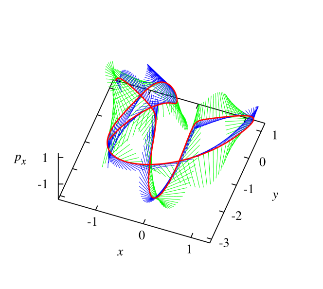
Figure 1: (Color online) Projection of a short spring-pendulum trajectory onto the $(x,y,p_{x})$-subspace. The blue and green lines represent projections of the covariant vectors $\bm{v}^{1}$ and $\bm{v}^{4}$, respectively, and give an impression of the respective unstable and stable manifolds along the trajectory. The time interval for this trajectory segment is 16 time units.

By the smooth (red) line in Fig. 1 we show a projection of a short trajectory into the three-dimensional subspace spanned by $x,y,p_{x}$. The covariant vector $\bm{v}^{1}$, which spans the unstable manifold, is indicated in green. Similarly, the covariant vector $\bm{v}^{4}$ spanning the stable manifold is shown in blue. Of course, these projected vectors are not of unit length. The figure may provide an intuitive understanding of the directions of maximum stretching or contraction of perturbations in phase space.

The time evolution of the polar components of $\bm{v}^{4}$ is depicted in Fig. 2. This vector was chosen for display since it is the most time consuming to compute and has a non-vanishing global exponent. The red lines are the results of a direct integration of Eqs. (21) within the polar environment, whereas the green lines are obtained by converting the Cartesian covariant vector $\bm{v}_{C}^{4}$ to its polar representation. As is indicated in Eq. (24), the sign is irrelevant since only the sense of direction counts. The same agreement is also obtained for the other covariant vectors (not shown).

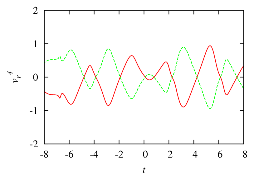
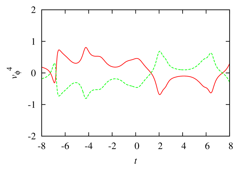
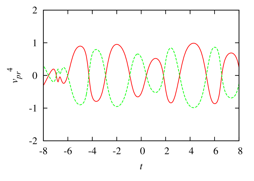
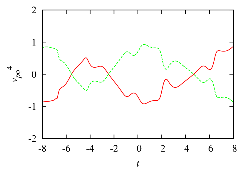
Figure 2: (Color online) Time evolution along the trajectory segment depicted in Fig. 1 of the four polar components $\delta r,\delta{\phi},\delta p_{r},\delta p_{\phi}$ (from top left to bottom right) for the covariant vector $\bm{v}_{P}^{4}$ spanning the stable manifold of the spring pendulum. The smooth (red) lines are obtained by direct integration with polar coordinates, whereas the dashed (green) curves were converted from the Cartesian representation.

The finite-time Lyapunov exponents (including the limiting case of local exponents) in the Cartesian and polar representations are also intimately connected. Let us consider a time element of duration $t_{n+1}-t_{n}=\tau$. The Cartesian covariant vector $\bm{v}_{C}^{\ell}(t_{n})$ evolves according to Eqs. (3) and (5) into a vector $\exp\left\{\Lambda_{C}^{\ell,\mbox{cov}}\tau\right\}\bm{v}_{C}^{\ell}(t_{n+1})$, which – according to Eq. (23) – may be transformed to the polar representation to give

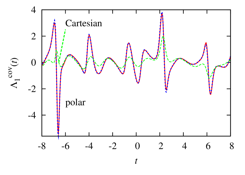
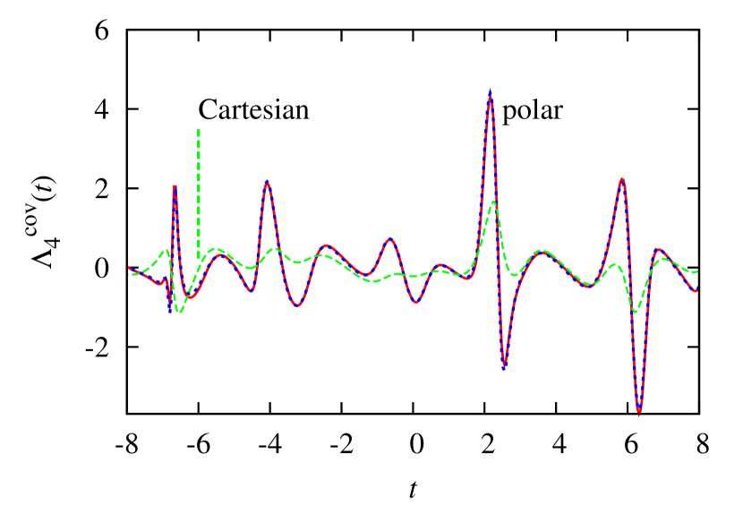
Figure 3: (Color online) Comparison of time dependent local covariant exponents for the unstable ($\ell=1$, left panel) and stable ($\ell=4$, right panel) manifolds of the spring pendulum. The smooth (red) lines are obtained by numerical integration of the polar equations of motion, the dotted (blue) lines by integration of the Cartesian equations of motion, followed by a conversion to the polar representation. The agreement is very good. For comparison, the corresponding Cartesian exponents, which are the basis of the conversion, are shown by the dotted (green) lines.

$$\exp\left(\Lambda_{C}^{\ell,\mbox{cov}}\tau\right){\cal M}(t_{n+1})\bm{v}_{C}^{\ell}(t_{n+1}).$$

Alternatively, $\bm{v}_{C}^{\ell}(t_{n})$ at $t_{n}$ may be first transformed to the polar representation, ${\cal M}(t_{n})\bm{v}_{C}^{\ell}(t_{n})$, and then be evolved in time to the end of the interval, which yields the vector

$$\exp\left(\Lambda_{P}^{\ell,\mbox{cov}}\tau\right)\big{\|}{\cal M}(t_{n})\bm{v}_{C}^{\ell}(t_{n})\big{\|}\bm{v}_{P}^{\ell}(t_{n+1}).$$

Equating these two expressions and taking the absolute value on both sides yields

$$\Lambda_{P}^{\ell,\mbox{cov}}=\Lambda_{C}^{\ell,\mbox{cov}}+\frac{1}{\tau}\ln\frac{\big{\|}{\cal M}(t_{n+1})\>\bm{v}_{C}^{\ell}(t_{n+1})\big{\|}}{\big{\|}{\cal M}(t_{n})\;\bm{v}_{C}^{\ell}(t_{n})\big{\|}}.$$ (25)

This provides the relation between the covariant local exponents in the two coordinate systems. Although expressed here in terms of the Cartesian and polar coordinates, the expressions (24) and (25) are completely general.

Eq. (25) clearly shows that the local exponents differ for different coordinate systems [4]. To test the last relation, we show by the smooth (red) lines in Fig. 3 the local (time-dependent) covariant exponents in the polar representation for the unstable manifold ($\ell=1$, left panel) and for the stable manifold ($\ell=4$, right panel) of the spring pendulum. They are obtained by direct integration of the motion equations (21) with polar coordinates. For comparison, the corresponding Cartesian exponents are plotted by the dashed (green) lines. If the latter are transformed to the polar representation, the dotted (blue) lines are obtained. The perfect match with the smooth (red) lines of the strictly polar approach asserts the validity of Eq. (25).

In Fig. 4 we show the (linear) growth rate of the covariance matrix for the logarithmic expansion $\tau\Lambda_{\ell}(\tau)$ as a function of the averaging interval $\tau$ for various representations. For the GS-vectors this rate matrix is given by [20]

$$D_{\ell\ell^{\prime}}^{\mbox{GS}}(\tau)=\lim_{\tau<\infty}\left[\left\langle\Lambda_{\ell}^{\makebox{GS}}(\tau)\Lambda_{\ell^{\prime}}^{\makebox{GS}}(\tau)\right\rangle-\bar{\lambda}_{\ell}\bar{\lambda}_{\ell^{\prime}}\right]\tau,$$ (26)

where we still have to distinguish the cases with Cartesian or polar coordinates. For covariant vectors the definition is given by Eq. (6). For clarity we restrict ourselves to matrix elements, which do not involve any of the vanishing Lyapunov exponents $\bar{\lambda}_{2}$ and $\bar{\lambda}_{3}$. The panel on the right-hand side is a magnification of the small-$\tau$ regime of the left panel. The elements for Gram-Schmidt FTLEs with Cartesian coordinates are indicated by red full points (case GS-C), those with polar coordinates by the blue full squares (case GS-P). Similarly, the elements involving covariant FTLEs with Cartesian coordinates are indicated by green crosses (case COV-C), those with polar coordinates by violet open circles (case COV-P). The following observations are made:

1. There exists the general symmetry $D_{11}(\tau)=D_{44}(\tau)$ and $D_{14}(\tau)=D_{41}(\tau)$ for any coordinate system and for any vector set used, be it Gram-Schmidt or covariant. Wheras the latter equality is trivial, the former is not in view of the fact that neither $\bm{v}^{1}$,$\bm{v}^{4}$ nor $\bm{g}^{1}$,$\bm{g}^{4}$ are simply related to each other.

2. $D_{11}(\tau)$ for GS-C and COV-C agree for all $\tau$, and similarly $D_{11}(\tau)$ for GS-P and COV-P. This is to be expected, since the covariant vector $\bm{v}_{1}$ and the GS vector ${\bm{g}_{1}}$ associated with the maximum exponent are identical by construction.

3. For small averaging intervals $\tau$, the fluctuations of the finite-time exponents as measured by $D_{11}(\tau)$ and $D_{14}(\tau)$ significantly differ for the cases GS-C and GS-P, as has been observed before [22]. A similar observation is made for the cases COV-C and COV-P. These differences gradually disappear for averaging times $\tau>10$.

4. The cross correlation $D_{14}(\tau)$ for the covariant and Gram-Schmidt vector sets differ enormously for small $\tau$, regardless what coordinate system is used. The difference is even larger between COV-P and GS-P than between COV-C and GS-C. By increasing $\tau$ these differences very slowly disappear.

5. From the left panel of Fig. 4 one infers that for $\tau>200$ all elements of the covariance matrix for the FTLEs become independent of the choice of the set of perturbation vectors and of the coordinate system. Thus, $\lim_{\tau\to\infty}D(\tau)$ becomes a dynamical invariant independent of the metric and parameterization [20]. For high-dimensional chaotic systems such a result has been interpreted as evidence for effective hyperbolicity of the dynamics and of the statistical insignificance of hyperbolic tangencies.

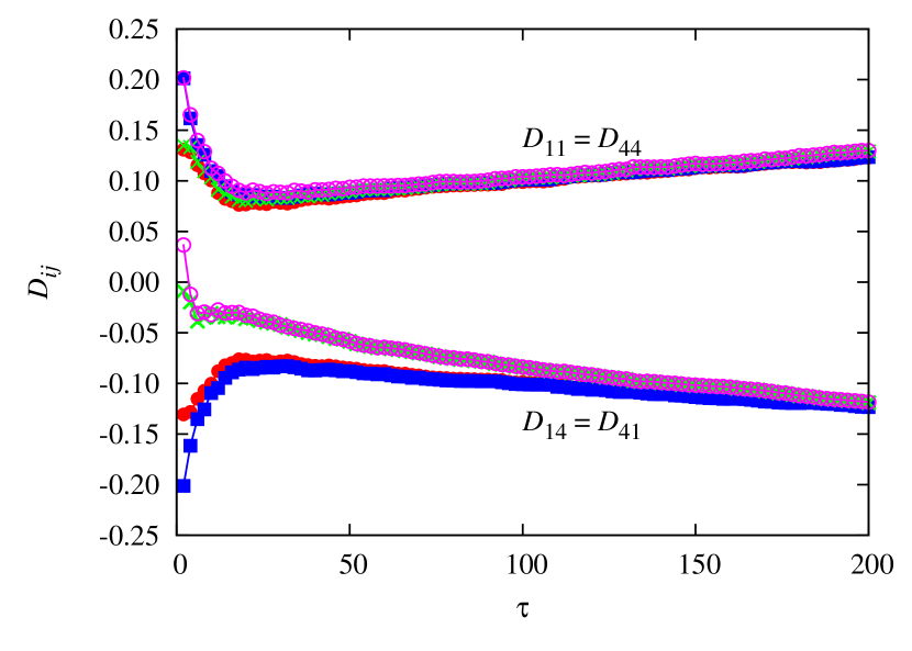
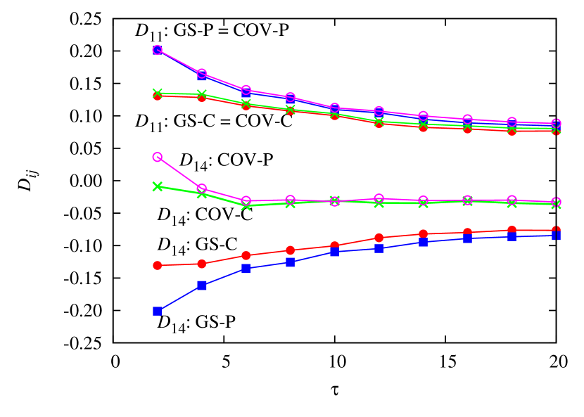
Figure 4: (Color online) Chaotic pendulum: $\tau$ dependence of the growth rate of the covariance matrix for the logarithmic expansion $\tau\Lambda_{\ell}(\tau)$. Only matrix elements not involving vanishing global exponents are shown. The panel on the right-hand side is a magnification of the small $\tau$ regime. Red full points: Cartesian coordinates and GS exponents (case GS-C); blue full squares: polar coordinates and GS exponents (case GS-P); green crosses: Cartesian coordinates and covariant exponents (case COV-C): violet open circles: polar coordinates and covariant exponents (case COV-P). In all cases the evolution is in the direction of the positive time axis.

4 The Hénon-Heiles system

As a second example, we consider the familiar Hénon-Heiles system [24] with a Hamiltonian in Cartesian coordinates

$$H_{C}=\frac{1}{2}(p_{x}^{2}+p_{y}^{2})+\frac{1}{2}(x^{2}+y^{2})+x^{2}y-\frac{1}{3}y^{3}.$$ (27)

For an energy $1/6$, the system is known to be chaotic (with a global Lyapunov spectrum $\{0.127_{7},0,0,-0.127_{7}\}$), where the trajectory visits most of the accessible phase space [25, 21]. The local Lyapunov exponents display the symplectic pairing symmetry Eq. (10-11), and the time reversal symmetry of Eq. (13), as is demonstrated in the respective left and right panels of Fig. 5.

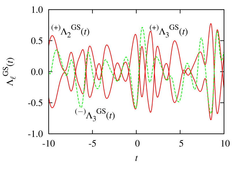
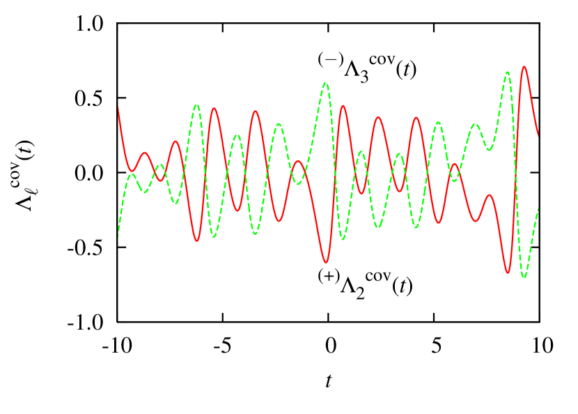
Figure 5: (Color online) Local Lyapunov exponents for the Hénon-Heiles system with energy $H=1/6$. Left panel: Illustration of the symplectic local pairing symmetry, Eq. (10-11), for the Gram-Schmidt (GS) exponents ${}^{(+)}\Lambda_{2}^{\mbox{GS}}$ and ${}^{(+)}\Lambda_{3}^{\mbox{GS}}$ (smooth red lines). The dimension of phase space $D=4$. The inequality Eq. (12) is demonstrated by the dashed green line for ${}^{(-)}\Lambda_{3}^{\mbox{GS}}$. Right panel: Verification of the time-reversal invariance property (13) for the local covariant exponents specified.

In polar coordinates defined by $x=r\cos\phi$ and $y=r\sin\phi$ the Hamiltonian becomes

$$H_{P}=\frac{p_{r}^{2}}{2}+\frac{p_{\phi}^{2}}{2r^{2}}+\frac{r^{2}}{2}+\frac{r^{3}}{3}\sin 3\phi,$$ (28)

where, as before, $p_{r}=\dot{r}$ and $p_{\phi}=r^{2}\dot{\phi}$ are the conjugate momenta. With an analysis completely analogous to that in the previous section for the spring pendulum, the covariant vectors in the polar representation may be obtained. Here, it suffices to present in Fig. 6 only results for the polar covariant vector $\bm{v}_{P}^{1}$ associated with the maximum exponent.

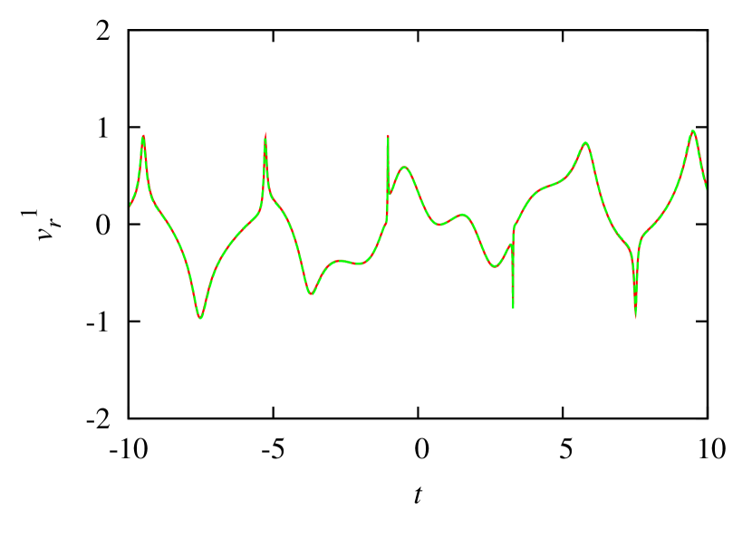
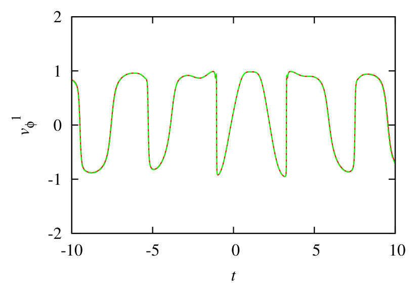
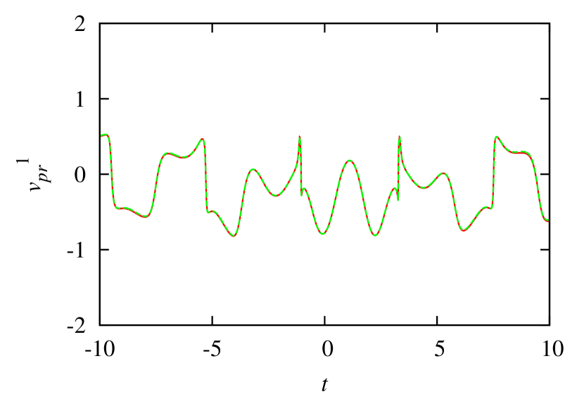
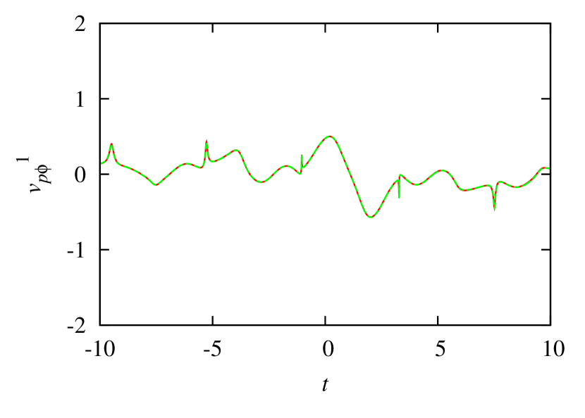
Figure 6: (Color online) Time evolution of the four polar components $\delta r,\delta{\phi},\delta p_{r},\delta p_{\phi}$ (from top left to bottom right) for the covariant vector $\bm{v}_{P}^{1}$ spanning the unstable manifold of the Hénon-Heiles system. In every panel two lines are shown. The smooth (red) lines are obtained by direct integration with polar coordinates, whereas the dashed (green) curves were converted from the Cartesian representation. Both lines agree and cannot be distinguished.

One observes that the covariant vectors are unique (up to the sign as the example in the previous section testifies), and that it does not matter what parameterization is used for their computation.

5 Résumé

There are many recent applications of Lyapunov vectors, which range from weather forecasting [28], geophysical applications [27], and studies of transport in turbulent flow [29, 30], to identifying and probing rare chaotic events by Lyapunov-weighted dynamics [31] and/or path sampling [32].

From the two sets of perturbation vectors commonly used - the orthonormal Gram-Schmidt vectors and the co-moving covariant vectors - the latter are more attractive from a physics point of view. They reflect time-reversal invariance and, as is shown here, they are unique and independent of the choice of the coordinate system. By uniqueness we mean that they are properties of the flow in tangent space, and when they are known in a particular frame, they may be easily converted to another. They provide a spanning set for the Oseledec splitting of the tangent space into a hierarchy of subspaces, each characterized by a well-defined Lyapunov exponent. In this sense, they are a property of the physical system. This is not the case for the more artificial ortho-normal Gram-Schmidt vectors, which are a mathematical device for computing volume changes of $d$-dimensional volume elements, $d\leq D$, in the $D$-dimensional phase space. Their advantage is that they are easier and faster to compute. According to the algorithm of Ginelli et al. [11], the computation of the covariant vectors at a phase-point ${\bf\Gamma}$ requires the knowledge of the Gram-Schmidt vectors for all points on the trajectory through ${\bf\Gamma}$ both in the past and the future [2]. Due to the availability of fast computers and programming techniques, rather high-dimensional systems have already been examined [4, 33, 14]

For many problems only the first Lyapunov vector associated with the maximum (global) exponent is required. Since the first Gram-Schmidt and the first covariant vectors always agree, one gets away with the fast computation of the first Gram-Schmidt vector, which is covariant. This advantage may dissolve again if the application requires the knowledge of the maximum local exponent together with its covariant vector. Due to possible exponent entanglement [13, 16] the maximum local exponent at a particular instant may belong, say, to the fifth vector. In such a case more than one covariant vectors need to be computed.

6 Acknowledgements

The author acknowledges stimulating discussions with Hadrien Bosetti [26] and William. G. Hoover and some very constructive remarks by an anonymous referee.

References

- [1] V.I. Oseledec, Trudy Moskow. Mat. Obshch. 19, 179, (1968) [Trans. Mosc. Math. Soc. 19, 197 (1968).
- [2] D. Ruelle, Publications Mathématiques de l’IHÉS 50, 27 (1979).
- [3] J.-P. Eckmann and D. Ruelle, Rev. Mod. Phys. 57, 617 (1985).
- [4] H.-l. Yang and G. Radons, Phys. Rev. E 82, 046204 (2010).
- [5] H.A. Posch and Wm. G. Hoover, Phys. Rev. A 38, 473 (1988).
- [6] I. Goldhirsch, P.-L. Sulem, and S.A. Orszag, Physica D 27, 311 (1987).
- [7] G. Benettin, L. Galgani, A. Giorgilli, and J.-M. Strelcyn, Meccanica 15, 21 (1980).
- [8] I. Shimada and T. Nagashima, Prog. Theor. Phys. 61, 1605 (1979).
- [9] A. Wolf, J.B. Swift, H.L. Swinney, and J.A. Vastano, Physica D 16, 285 (1985).
- [10] C. Dellago, H.A.Posch, and W. G. Hoover, Phys. Rev. E 53, 1485 (1996).
- [11] F. Ginelli, P. Poggi, A. Turchi, H. Chaté, R. Livi, and A. Politi, Phys. Rev. Lett. 99, 130601 (2007).
- [12] C.L. Wolfe and R.M. Samelson, Tellus 59A, 355 (2007).
- [13] H.-l. Yang and G. Radons, Phys. Rev. Lett. 100, 024101 (2008).
- [14] H.-l. Yang, K.A. Takeuchi, F. Ginelli, h. Chaté, and G. Radons, Phys. Rev. Lett., 102, 074102 (2009).
- [15] H. Bosetti and H.A. Posch, Chem. Phys. 375, 296 (2010).
- [16] H. Bosetti, H.A. Posch, C. Dellago, and Wm.G. Hoover, Phys. Rev. E 82, 046218 (2010).
- [17] H.A. Posch and H. Bosetti, ”Covariant Lyapunov vectors and local exponents”, in Non-equilibrium Statistical Physics Today, Proc. of the 11th Granada Seminar on Computational and Theoretical Physics, edited by P.L. Garrido, J. Marro, and F. de los Santos, p. 230, American Institute of Physics (AIP Conference Proceedings), Melville, New York, 2011.
- [18] Wm. G. Hoover, and C. Hoover, Commun. Nonlinear Sci. Numer. Simulat., in press (2011); arXiv 1106.2367.
- [19] K.A. Takeuchi, H.-l. Yang, F. Ginelli, G. Radons, and H. Chaté, Phys. Rev. E 84, 046214 (2011).
- [20] P.V. Kuptsov and A. Politi, Phys. Rev. Lett.107, 114101 (2011).
- [21] R. Ramaswamy, Eur. Phys. J. B 29, 339 (2002).
- [22] H.A. Posch, Wm.G. Hoover,and C.G. Hoover, Phys.Rev. A 41, 2999 (1990).
- [23] C. Dellago and Wm.G. Hoover, Phys. Lett. A 268, 330 (2000).
- [24] M. Hénon, Comm. Mathem. Phys. 50, 69 (1976).
- [25] A.J. Lichtenberg and M.A. Lieberman, Regular and Stochastic Motion, Springer, New York, 1983.
- [26] H. Bosetti, On the microscopic dynamics of particle systems in and out of thermal equilibrium, Ph.D.-thesis, University of Vienna, 2011.
- [27] Ch.L. Wolfe and R.M.Samelson, Tellus 59A, 355 (2007).
- [28] B. Legras and R Vautard, Predictability 1, European Centre for Medium-Range Weather Forecasts, 143 (1996).
- [29] E. Balkovsky and A. Fouxon, Phys. Rev. E 60, 4164 (1999).
- [30] A. Fouxon and V. Lebedev, Phys. Fluids 15, 2060 (2003).
- [31] J. Tailleur and J. Kurchan, Nature Physics, 3, 203 (2007).
- [32] P. Geiger and C. Dellago, Chem. Phys. 375, 309 (2010).
- [33] H. Bosetti and H.A. Posch, submitted (2012); arXive:1111. 5951.