Galactic S Stars: Investigations of Color, Motion, and Spectral Features
Abstract
Known bright S stars, recognized as such by their enhanced s-process abundances and C/O ratio, are typically members of the asymptotic giant branch (AGB) or the red giant branch (RGB). Few modern digital spectra for these objects have been published, from which intermediate resolution spectral indices and classifications could be derived. For published S stars we find accurate positions using the Two-Micron All Sky Survey (2MASS), and use the FAST spectrograph of the Tillinghast reflector on Mt. Hopkins to obtain the spectra of 57 objects. We make available a digital S star spectral atlas consisting of 14 spectra of S stars with diverse spectral features. We define and derive basic spectral indices that can help distinguish S stars from late-type (M) giants and carbon stars. We convolve all our spectra with the Sloan Digital Sky Survey (SDSS) bandpasses, and employ the resulting magnitudes together with 2MASS mags to investigate S star colors. These objects have colors similar to carbon and M stars, and are therefore difficult to distinguish by color alone. Using near and mid-infrared colors from IRAS and AKARI, we identify some of the stars as intrinsic (AGB) or extrinsic (with abundances enhanced by past mass-transfer). We also use band and 2MASS magnitudes to calculate a temperature index for stars in the sample. We analyze the proper motions and parallaxes of our sample stars to determine upper and lower limit absolute magnitudes and distances, and confirm that most are probably giants.
Subject headings:
Stars: abundances, AGB and post-AGB, carbon1. INTRODUCTION
When a low to intermediate mass star exhausts its core supply of hydrogen, contraction and heating of the core causes the outer layers of the star to expand and cool, whereby the star becomes a red giant (RG) with an average effective temperature of 5000 K or lower. Once the core temperature rises to about 3 K, helium burning begins, and the stellar surface contracts and heats creating the horizontal branch (for Population II) or red clump (for Population I) stars on the color-magnitude diagram. Completion of core helium burning and the start of helium shell burning returns the star to a luminous, cooler phase as it evolves onto the asymptotic giant branch (early- or E-AGB) where the star greatly expands and the hydrogen shell is (almost) extinguished. Later, as the He-burning shell approaches the H-He discontinuity, a phase of double shell burning begins. Recurrent thermal instabilities in this thermally-pulsing asymptotic giant branch (TP-AGB) phase are driven by helium shell flashes, periodic thermonuclear runaway events in the He-shell (Iben & Renzini, 1983) The energy released by these pulses expand the star, whereby the hydrogen shell is again basically extinguished during some time. A third dredge up might then occur, and afterward the hydrogen shell will re-ignite (and a new thermal pulse will occur). During these short-lived pulses, nucleosynthesis products from combined H-shell and He-shell burning are dredged up to the outer layers of the star. The complex details of the dredge-up and its outcome are strongly mass-dependent (Herwig 2005 and references therein), but generally speaking, surface abundance enhancements result in C, He, and the -process elements, including Ba, La, Zr, and Y.
S and Carbon (C) stars are traditionally thought to be members of the TP-AGB. In addition to possibly elevated C/O ratios, these stars exhibit other unique spectral characteristics as a result of the dredge-up. While M giants often exhibit titanium oxide (TiO) absorption bands, both carbon and zirconium have a higher affinity to free oxygen. Therefore, a higher C/O ratio also results in the disappearance of TiO bands and the appearance of zirconium oxide (ZrO) bands. S stars are therefore distinguished primarily by their ZrO bands, while C stars show strong C2 and CN bands. The S star spectral class is divided into three subtypes (in order of increasing carbon abundance): MS, S, and SC stars. Classification into one particular class is difficult, but is generally based on the C/O ratio and the relative strengths of TiO, ZrO, and CN molecular absorption bands. Overall, a star in the S star class is generally defined as having a C/O ratio (r) of and strong ZrO absorption features (Jorissen et al., 1993; Van Eck et al., 2010). Pure S stars are those that show only ZrO bands, and no TiO bands (Wyckoff & Clegg, 1978). Classification is complicated by the fact that increased intensity of the ZrO bands may be due to an excess of Zr, rather than being exclusively tied to the C/O ratio (Plez et al., 2003). Furthermore, many AGB S and C giants are highly variable, and since the strength of molecular bands depends on the effective temperature and surface gravity of the star, spectral type can vary significantly with time.
S stars whose spectra show lines of the short-lived element -process technetium (Tc) are known as ”intrinsic” S stars, and are most likely be members of the TP-AGB. 99Tc is only produced by the -process, while the star is on the AGB. Since the half-life of 99Tc is only 2.13 x 10⁵ years, and the average duration of the AGB phase of stellar evolution is roughly 1 Myr, stars exhibiting significant abundances of technetium are almost certainly members of the AGB (Van Eck & Jorissen, 2000). By contrast, technetium-poor S stars are known as ”extrinsic” S stars. These stars are likely to be part of binary systems and their unusual chemical abundances probably originated in a past mass-transfer episode (Van Eck & Jorissen, 2000). The present extrinsic S star likely once accreted -process rich material from its companion, a TP-AGB star at the time that has since evolved into a white dwarf. Extrinsic S stars therefore display enriched -process elements, despite having never produced these elements themselves. Most known extrinsic S stars are assumed to be members of the red giant branch (RGB). They can sometimes be distinguished from intrinsic S stars on the basis of color, because they do not necessarily show the red excess characteristic of stars on the AGB. While all currently known extrinsic S stars are thought to be giants, these definitions open up the possibility of extrinsic S stars on the main sequence (hereafter referred to as dwarf S stars) that have previously accreted -process material and carbon from a companion but whose Tc has since decayed. Analogous to the dwarf C stars (Green et al., 1991), a faint S star could be shown to be a dwarf if it has a sufficiently large parallax or proper motion; a large proper motion predicts a tangential velocity greater than the Galactic escape speed unless the object is faint and nearby.
S stars are very similar to C stars, with the major difference being a slightly lower C/O ratio. Faint high galactic latitude carbon (FHLC) stars were once assumed be giant stars at large distances. In 1977, however, G77-61 was discovered to have high proper motion and an upper limit absolute magnitude of +9.6, therefore making it the first known carbon dwarf star (Dahn et al., 1977). In this case, the term dwarf refers to a star on the main sequence. Green et al. (1991) discovered four other dwarf carbon (dC) stars using techniques that selected known carbon stars for high proper motion. Now, well over 100 dwarf carbon stars are known (Downes et al., 2004). The local space density of dCs is far higher than all types of C giants combined (Green et al., 1992). Therefore, contrary to previous assumptions, dwarf C stars are the numerically dominant type of carbon star in the Galaxy.
Since dC stars are now known to be so common, we have begun a search for dwarf S stars. There is little reason to believe that dwarf S stars should not exist. In fact, they may be more abundant than dC stars, since less carbon enhancement is required to produce an S dwarf as compared to a C dwarf. On the other hand, if the range of abundance ratios that produces the characteristic features of S stars is narrow, they may be quite rare. Furthermore, the range of C/O ratios that produces S star spectral features may be different for giants and dwarfs, given the higher gravities and larger temperature ranges in dwarfs.
We use medium-resolution digital spectra of known S stars (which are probably giants) to generate corresponding Sloan Digital Sky Survey (SDSS) colors, to see whether their colors might be sufficiently distinctive to search for additional S stars in the SDSS with reasonable efficiency. We also use the FAST spectra to investigate molecular band spectral indices for classification.
Our paper is organized as follows: in §2 we briefly review the observations and our data reduction and processing procedures. In section §3 we describe the production of a spectral atlas of S stars, and derive spectral indices from the molecular band strengths in §4. In §5 we describe the generation of SDSS colors and analyze the overall colors of the FAST sample in order to determine whether an efficient color selection for S stars exist. In §6 we discuss techniques for distinguishing intrinsic and extrinsic S stars and apply them to the FAST sample. In §8 we analyze the parallaxes and proper motions of S stars in the sample to characterize upper and lower limit magnitudes and distances. We use colors to generate approximate temperature indices for S stars in §7. In §9 we summarize our results and present our conclusions.
2. OBSERVATIONS
2.1. Sample Selection
The largest spectral catalog of S stars is Stephenson’s second edition (1984), which includes 1347 objects with poorly known positions. The stars in this catalog were originally identified from blue, red, and infrared objective prism plates. The majority of the S stars were discovered on the basis of the red system of ZrO absorption bands, with a bandhead around 6474 Å. Since the Stephenson catalog has a limiting V magnitude of approximately 11.5, most of the objects are highly saturated in the SDSS and reliable u, g, r, i, and z magnitudes have not been found for any known S stars. We assembled a sample of known S giants in order to generate likely g and r colors for S giants and dwarfs. These constraints on colors of S giants and dwarfs could allow us to search the SDSS and 2MASS catalogs for potential dwarf S star candidates.
To choose the stars making up the sample, we selected high Galactic latitude ( deg), northern ( deg) S stars from Stephenson’s catalog. This ensures that our sample is accessible from Mt. Hopkins, and also decreases problems of object confusion or reddening. We then correlated the sample from Stephenson’s catalog with 2MASS to find improved positions for most objects; accuracy of the original positions is typically , but commonly as poor as 20″. The final sample list, which includes 57 objects, can be found in Table 1. Each object is accompanied by its identification in both the Stephenson and 2MASS catalogs, as well as its position. Since many of these stars are known to be variable, we include the date of observation. We include other common identifiers for each target and a published spectral type, if available. We include our calculated temperature index for the star, which is discussed further in §7. Spectral types and temperature indices of the S stars in the sample may vary as a function of time, because the stars themselves do. When spectral types for different epochs were available, we match the magnitudes of the epochs to those listed in Table 2 to find the spectral type. Finally, we include identifications of some stars as intrinsic or extrinsic (denoted respectively by ’i’ and ’e’) from Yang et al. (2006) or from our own calculations based on AKARI magnitudes. For more information regarding the intrinsic/extrinsic identifications, see §6.
2.2. Observations and Data Reduction
Spectra were obtained using the FAST instrument on the 1.5 m Tillinghast reflector on Mt. Hopkins. FAST produces medium-resolution optical wavelength spectra, spanning a wavelength range from 3474 to 7418 Å. All data were taken using the 3” slit and a 300 lines mm-1 grating, producing a resolution of 1,000 at 6,000Å. Exposure times varied widely based on the magnitude of the star, but ranged from 3 to 300 s. The two-dimesional spectra were bias-subtracted and flat-fielded by the observatory standard data reduction procedure. After extraction, and the one-dimensional spectra were wavelength calibrated.
We used standard star spectra taken each night of the observations to produce sensitivity curves and flux calibrated spectra. An extinction correction file from Kitt Peak National Observatory was also applied to correct for major atmospheric effects. The standard calibration stars used to create the sensitivity curve are BD+26 2606, BD+33 2642, BD+17 4708, Feige 34, and HD 19445. Flux calibration and extinction corrections were performed using the onedspec package and the calibrate task in IRAF. We used a combination of observatory logs and night-to-night comparison of the sensitivity function to determine whether the calibrated target spectra were reliable enough to use in color analysis. We rejected some of the initial data sample based on concerns about non-photometric conditions and atmospheric distortion. Other nights are included in the final data for analysis because while the data may not be entirely photometric, it remains reliable enough for color analysis because of the non-wavelength dependent nature of most remaining distortions. We discuss the errors in our derived SDSS colors further in §5.1.
Many of the targets are luminous enough in red wavelengths that longer exposure times cause parts of the spectrum to saturate. The wavelengths from 6000 Å onward are of particular concern. However, shorter exposure times limited the amount of information we could derive from wavelengths below 4500 Å because of low signal-to-noise ratios. To create an S star spectral atlas, when possible we interpolated between two different exposure times: a shorter exposure time that produced accurate, unsaturated spectra at the longer wavelengths, and a longer exposure that resulted in higher signal-to-noise at shorter wavelengths. Generally, we determined by hand which spectra were reliable in a particular wavelength region by comparing multiple exposure times and examining long exposures for nonlinear behavior in areas from 6000 Å onward. For stars with only one available exposure time, we rejected a star as saturated if the counts exceeded 60,000. After interpolating between spectra to eliminate saturated regions and rejecting some data, we were left with 46 S star spectra.
3. Creating the Spectral Atlas
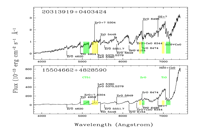
We use S star line identifications (Wyckoff & Clegg, 1978) to identify major spectral features and select objects with unique characteristics to include in the final spectral atlas, which includes 14 objects marked in Table 1. The objects were chosen to be a representative sample of the larger FAST sample, which includes many fundamentally similar objects. Two sample spectra with associated molecular line identifications are plotted in Figure 1. While the spectra display the same molecular bands, most notably those associated with ZrO, they have different overall colors, which may be due to differences in abundances and/or effective temperatures. We also note that these spectra show some TiO bands, indicating that they are not pure S stars, but instead probably belong to the MS classification. The appearance of TiO bands indicates the possibility of a C/O ratio slightly less than 0.95. The creation of a spectral atlas allows for greater investigation into the similarities and differences within the S star class. For instance, some members of the spectral atlas exhibit, in addition to prominent ZrO features, H, H, and H emission lines. The presence of these emission lines indicates that these objects are almost certainly AGB stars, e.g., Miras. The spectral atlas is made available digitally as 14 individual FITS files via this journal.
4. Spectral Indices of S Stars
We can immediately use the first digital spectral atlas of S stars to derive some medium-resolution spectral indices, potentially useful to classify stars as M, S, or C even where they may have very similar broadband colors. Apart from our own FAST spectra of 48 S stars, we use M giants from the Indo-US spectral atlas (Valdes F., et al., 2004). We use eight carbon star spectra also obtained with the FAST for a separate project (Green et al. 2011, in preparation). These latter spectra span a wide range of spectral band strengths, but are selected from the SDSS color wedge defined by Margon, B., et al. (2002).
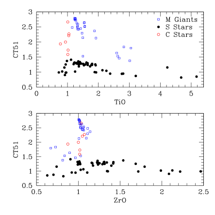
We defined three indices, one each for TiO, ZrO, and C2. We follow the basic premise of using ratios of mean flux per Ångström across key molecular bands, so that spectra of differing resolution should yield similar results. We use a neighboring comparison region for each band, so that sensitivity to broadband flux calibration is minimized. For the ZrO index, we divide the mean flux Å across 6400 – 6460Å (ZrO off-band) by that between 6475 – 6535Å (ZrO band). For the TiO index, we use mean Å-1 flux from 7065 – 7175Å (TiO band) divided by 6965 – 7028Å (TiO off-band). The C index is derived from 5025 – 5175 Å (C2 band) and 5238 – 5390Å (off-band). Thus, lower flux in the denominator caused by strong molecular bands yields a larger spectral index value. We note that the C index near 5100Å can also be substantially contaminated by TiO, so we label it “CT51” hereafter. At least within this representative sample of stars, a combination of these indices yields a preliminary S star classification, as shown in Figure 2. The objects most reliably classified as S stars would have ZrO index and C2 index .
5. Color Selection of S Stars
5.1. Generating SDSS and 2MASS Colors
To use the SDSS database to find likely candidates for both S giants and dwarfs, we need reliable colors for our objects in as many SDSS bandpasses as possible. The spectra from FAST cover the bandpasses for the and filters completely, and we are thus able to convolve our spectra with these bandpasses and generate SDSS colors. Each of the FAST spectra contains 2681 data points, with approximate wavelength separation of 1.47 Å. To convolve the spectra with the filter transmission curves, we use linear interpolation between transmission values to match a transmission constant to each data point in the spectrum. Once we find a transmission constant for each wavelength, we normalize the transmission curve and then convolve the spectrum with the transmission curve. We use the IRAF task calcphot in the synphot package of stsdas to convolve the spectra with the bandpasses and obtain SDSS colors from our spectra. The SDSS bandpass curves are taken from information made available by the SDSS consortium (Fukugita et al., 1996). As with all SDSS magnitudes, the resultant magnitudes are in the AB magnitude system. By including both SDSS and 2MASS bandpasses, we are able to calculate 10 unique colors.
We also conduct error analysis on the derived SDSS colors using the standard star spectra and the known g-r colors and r magnitudes for BD+26 2606, BD+33 2642, BD+28 4211, and BD+174708. These colors are published by the SDSS consortium, and allow us to constrain our errors in both the magnitudes and colors (Smith et al., 2002). We calculate the difference between measured and standard and magnitudes, and find a standard deviation of mag for the band and mag for the band. While these seem high and would suggest, via propagation of errors, a correspondingly high error in our colors (on the order of 0.4 mag), we find a standard deviation of only mag for the color. The value was calculated by comparing the derived colors for the standard stars to the known colors from the SDSS Data Release 5 standard star network (Smith et al., 2002). The low value in the uncertainty of our colors is probably due to the fact that while our spectra may not be absolutely photometrically calibrated, many of the remaining distortions are not wavelength dependent and therefore cancel out during color calculation. Examples of remaining distortions include slit losses, an incomplete cancellation of the telluric spectrum or a thin cloud layer that dims the overall flux at all wavelengths. So while individual magnitudes remain unreliable at best, the errors in the derived color are comparable to color errors in 2MASS and are thus reliable enough for our analysis. The 2MASS magnitude errors for our sample have a wide range dependent upon the reliability of the photometry for a particular night, but generally range from 0.02 magnitudes up to about 0.2 magnitudes. Colors calculated from 2MASS magnitudes thus have errors comparable to the derived SDSS colors.
5.2. Color Selection Analysis and Criteria
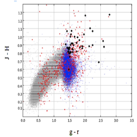
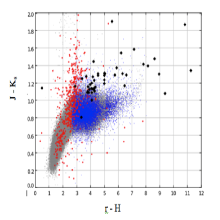
The initial aim of the project was to select for S stars based on their SDSS and 2MASS colors. To achieve this goal, we derive and magnitudes for the stars making up our sample and combine with the known 2MASS magnitudes to construct a total of 10 unique colors. The , , and 2MASS magnitudes, along with band, IRAS, and AKARI photometry where available, are presented in Table 2. Many of these colors, however, are ultimately unhelpful for analysis purposes because the colors of known S stars cover several magnitudes. Such a wide spread in magnitudes does not allow for efficient discovery of the S stars based on color. In other color combinations, the S stars are not well distinguished from the stellar locus, so selection based on color is contaminated by large numbers of stars from the main sequence. We find that the most useful color combinations are , , and because in these colors, the FAST S stars sample is well distinguished from the stellar locus. We compare these colors with those found for general SDSS stars, by overplotting some 300,000 SDSS/2MASS matches of (Covey et al., 2007), which they used to parametrize the stellar locus in terms of color. In Figure 3, we present two color-color diagrams in which the S giants from the FAST sample are best separated from the stellar locus. The first shows the comparison of color and color, while the second shows the comparison and color.
However, the S giants that comprise the FAST sample, by virtue of their location on the TP-AGB or RGB, have similar colors and effective temperatures to M giants. In Figure 3, we also examine colors for M giants and dwarfs matched in the SDSS and 2MASS surveys. While the M giants are very few in number (due to the depth of both of these surveys, many nearby M giant targets are saturated), we can immediately see that S stars and M stars lie in essentially the same area of color space. We also include C stars on the color-color diagrams, since they follow evolutionary paths similar to S stars and also have enhanced abundances. The S stars of the FAST sample, while well-distinguished from the overall stellar locus on both color-color diagrams, are particularly difficult to distinguish from C stars on the versus diagram. On the plot comparing to , S stars can be distinguished reasonably well from the bulk of the M star population using and . Given the biases in the current sample of S stars, it is difficult to determine the efficiency of this selection, but this region on the color-color plot appears to be the least contaminated by M and C stars. Spectroscopy for a sample of perhaps 100 stars in this color region could directly test the efficiency of this color selection.
6. Distinguishing Intrinsic and Extrinsic S Stars
6.1. Techniques
Distinguishing intrinsic and extrinsic S stars is difficult without high-resolution spectroscopy, where direct detection of Tc is possible. However, as presented in Van Eck and Jorrissen (2000), there are other measurements which serve to segregate the two types with reasonable statistical accuracy. Since extrinsic S stars are generally on the RGB (or early AGB), they cluster closer to the main sequence than intrinsic S stars in terms of color. Stars on the AGB generally show a red excess which is absent on the RGB. However, Van Eck and Jorissen (2000) find that blue excursions of Mira variables, which make up a significant proportion of intrinsic S stars, make the two classes difficult to distinguish based on distance from the main sequence alone. Additionally, intrinsic and extrinsic S stars have been shown to segregate well in a (, ) diagram (Groenewegen, 1993; Jorissen et al., 1993). These colors are based on IRAS photometry, which is available for many of the stars in the FAST sample. IRAS magnitudes in these bands are presented in Table 2 for 37 stars (with two bands available for 29). Identifications of many of the S stars in the FAST sample as intrinsic or extrinsic are included in Table 1. All such identifications not marked with an asterisk are from Yang et al. (2006). Classification of most of the S stars in our sample is inconclusive because of their intermediate positions in the color-color diagrams. However, this IR technique remains the most efficient photometric classification method known to determine whether S stars are intrinsic or extrinsic.
We also use results from Vanture et al. (private communication), which indicate that S stars presenting Li in their spectra are intrinsic S stars. Lithium in stars is destroyed at fairly low temperatures (Bodenheimer, 1965) but can be produced by the Cameron-Fowler mechanism, in high luminosity () TP-AGB stars via hot bottom burning. Since, as mentioned above, extrinsic S stars are often less evolved along the giant branch than intrinsic S stars, they generally lack any evidence for the resonance line Li 6707Å (Vanture et al. 2011, in preparation). We compare the list of S stars with and without Li detections to our FAST sample and analyze them for the Li 6707 Å feature. Unfortunately, we find that this line cannot be reliably detected with spectra of our resolution and S/N.
6.2. Identification Using AKARI Magnitudes
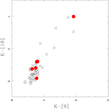
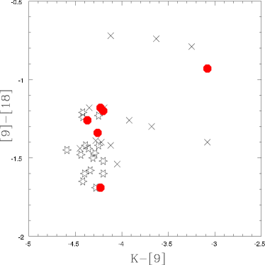
The AKARI satellite surveyed much of the sky in both near and far infrared bands. We use flux data collected by AKARI in the S9W and L18W bandpasses to find infrared magnitudes for six objects in the FAST sample without available IRAS colors (Murakami et al., 2007; Ishihara et al., 2010). The S9W and L18W bandpasses are qualitatively similar to the IRAS 12 and 25 micron bandpasses. All available AKARI magnitudes are presented in Table 2, for 52 stars (with two bands available for 35). Since the zero magnitude fluxes for these bandpasses are not well established, all magnitudes are presented on the AB system. In Figure 4, we show two color-color diagrams comparing intrinsic and extrinsic stars using , , and colors. S stars previously classified as intrinsic vs. extrinsic are shown in black, with others plotted in red.
From the AKARI magnitudes and plots, we are able to identify an additional two stars in the sample as intrinsic or extrinsic. We identify 22315839+0201206 as an extrinsic S star. This star has a value of mag and a value of mag. This places it in the extreme lower left corner of the color-color diagram comparing color to color, far away from any known intrinsic stars but close to many known extrinsic stars. Similarly, we are able to identify 19364937+5011597 as an intrinsic S star on the basis of color. This star has a value of only mag, and a value of mag. This places it in the upper right-hand corner of the plot comparing and and color, far away from the cluster of extrinsic S stars. The four other stars for which we have no classification (03505704+0654325, 10505517+0429583, 13211873+4359136, and 16370314+0722207) cluster close to the transition between intrinsic and extrinsic S stars in all three color comparisons, meaning that we cannot confidently identify these with either class of stars. We include our additional identifications in Table 1, marked with an asterisk to distinguish them from those from Yang et al. (2006).
7. Calculating Temperature Indices
7.1. Using Colors to Determine Temperature
As mentioned before, S stars cover a wide range of spectral types and effective temperatures. However, they generally have effective temperatures similar to those of M giants. The starting point for classifying the spectral type and temperatures of our S stars, therefore, is to calculate a temperature index using M-giant criteria (Gray and Corvally, 2009). Houdashelt et al. (2000) use a grid of stellar models to calibrate a relation between color and temperature index for M stars. Their analysis uses CIT/CTIO colors and . We find magnitudes for some of the FAST sample using Simbad. We also convert the 2MASS Ks magnitudes and colors using the following relations from Carpenter (2001):111Updated at http://www.astro.caltech.edu/j̃mc/2mass/v3/transformations
| (1) |
We then use the temperature index/color relation to assign a preliminary temperature index to the stars in the FAST sample. Where possible, we use the relation, since this is specified by the authors as the most temperature sensitive. When there is no magnitude available, we use the relation (Houdashelt et al., 2000).
7.2. Results of Temperature Analysis
Results of this analysis are presented in Table 1. These temperature indices should be treated with caution, since many of the stars in the FAST sample are highly variable. Furthermore, differences in C/O ratios, may lead to temperature errors up to 400 K (Van Eck et al., 2010). However, the preliminary classification gives us a rough idea of the relative effective temperatures of the S stars. We find that the average temperature index of the stars in the sample is 5, which in M giants corresponds to an effective temperature of roughly 3500 K (Houdashelt et al., 2000). In Table 1, we also present known spectral types from Keenan & Boeshaar (1980), which include temperature indices for the S stars. We find reasonably good agreement between our calculated temperature indices and those presented as part of the spectral type. Differences between our temperature index and those included as part of the published spectral types are within the range of variability of the star. We also note that since we do not have a reliable color/temperature relation for stars with a temperature index greater than 7, we present all of these classes as 7+. We also find reasonably good agreement (within one temperature index) between the values using and those derived using .
We also conduct a preliminary analysis on possible correlations between the intrinsic/extrinsic distinction and the temperature indices. We find that the average temperature index of the intrinsic stars is , while the average temperature index of extrinsic stars is . Therefore, while the mean temperature index shows some differences, this measurement alone is not statistically significant. A larger sample would be needed to determine the validity of differences between average effective temperature between intrinsic and extrinsic S stars. The temperature indices of S stars in general are insufficient to classify them as intrinsic or extrinsic, except for the reddest objects.
8. Parallax, Proper Motion, and Absolute Magnitude
8.1. Parallax Analysis
Four of the stars in the original FAST sample have reliable parallax measurements (defined as a parallax detection at the level) available from the Hipparcos survey (Perryman et al., 1997), so calculation of the absolute magnitude of these stars in the and bands is possible. We calculate the error in our absolute magnitudes using the presented error in the parallax measurements and assuming apparent magnitude error values of and . Results of this analysis are given in Table 3. We note the calculated absolute and magnitudes, as well as the associated errors. Objects are identified using the 2MASS Identifier, and the parallax and associated error as given by the Hipparcos catalog are also included. We can immediately identify each of these four objects as asympotic or red giant branch members: if they were dwarf stars of the same spectral type, we would expect magnitudes in the and of +5 or higher, as opposed to the derived values, which center around 0.
8.2. Proper Motion Analysis
We also find that some stars in the original FAST sample display significant (again, ) proper motions. The proper motions are available in the Tycho-2 catalogue (Høg et al., 1997). Of these, we have reliable and photometry for 16 objects. Given the proper motion and assuming that all objects are moving at total space velocities less than the Galactic escape velocity, we can derive an upper limit on the distance, and thus also constrain the absolute magnitudes of the objects. To derive an approximate distance (), we use the equation:
| (2) | ||||
| (3) | ||||
| (4) |
where is the proper motion of the object measured in radians per year, is the transverse velocity of the object, and is the Galactic escape velocity. We take the Galactic escape velocity to be 545 km/s (Smith et al., 2007), which is equivalent to 0.0056 parsecs per year. The distance constraint is only an upper limit because we neglect radial velocities. However, we note that our rvsao measurements generally yield small radial velocities (50 km/s) for the S star sample. We then use the same formulas presented above to derive and absolute magnitudes and associated errors. These and absolute magnitudes essentially represent the brightest the object concerned could be, considering its proper motion and assuming that all observed objects are gravitationally bound members of the Milky Way. Results of the analysis are presented in Table 4. We can immediately see from these lower bound magnitudes that these objects could be RGB or AGB stars - even considering that the actual magnitudes are probably significantly fainter. For the sample of 16 stars, we find that the average lower limit on the absolute magnitude is mag, correspondingly mag. Cool dwarf stars generally have and absolute magnitudes greater than +8 mag (Dahn et al., 1977; Vyssotsky, 1947) We conclude that all 16 objects displaying significant proper motions could be giants.
8.3. Lower Limit Distances
To further bear out this analysis, we also determine a lower limit on the distance for these objects by assuming (conversely to above) that they do have a dwarf magnitude. We take the approximate absolute -band magnitude for an M dwarf star to be = 10 mag and the absolute -band magnitude to be = 9 mag (Dahn et al., 1977; Vyssotsky, 1947). This method can be applied to the entire sample, because it does not rely on proper motion or parallax measurements. We find that most of these objects, were they to have typical dwarf magnitudes, would be within 25 pc of us. This distance would almost guarantee that these objects would have detectable parallax and proper motion. For instance, assuming extrinsic S stars are a mostly spheroid population (like dC or CH stars: see Green et al. (1994) and Bergeat et al. (2002)) with velocity of km/s relative to the Sun (Sirko et al., 2004), the typical proper motion for a star 25 pc away would be on the order of 2.25 mas/yr. Additionally, such stars would have a parallax on the order of 40 mas. Since such a parallax would be easily detectable by Hipparcos, these lower limit distances therefore also suggest that the stars of the FAST sample are likely to be giants or AGB stars.
9. Summary and Conclusions
Using a sample of 57 medium-resolution S star spectra taken with the FAST spectrograph, we create a spectral atlas of S stars comprised of 14 objects that span a range of spectral types within the MS, S, and SC classes. The atlas is published as a collection of 1-D FITS files via this journal. After generating and SDSS magnitudes from the spectra, we find that the SDSS magnitudes in the and bands, combined with , , and magnitudes from the 2MASS catalog for S stars may with further confirmation allow for reasonably efficient color selection of these objects from the SDSS and 2MASS catalogs. We use previously published data to identify some of the stars in the sample as intrinsic or extrinsic stars, and find that the fraction of extrinsic S stars in the sample is approximately . We also assign temperature indices to the stars in the sample based on the M star scale of temperature indices. We find that much of the S star sample falls at temperature index 4 or above, meaning that the effective temperatures of most of these stars are well below 5000 K. We also analyze objects in the FAST sample with detectable parallaxes and proper motions to generate absolute magnitude limits, as well as lower limit distances based on assumed dwarf magnitudes. This analysis bears out our initial assumption that the FAST sample is primarily composed of giant stars, either on the AGB or RGB.
10. Acknowledgements
Many thanks to the referee for a thorough reading. We are grateful to Kevin Covey for the use of the high-quality sample of SDSS/2MASS matches. Also, thanks to Warren Brown and Mukremin Kilic, who provided many helpful discussions and hints on color selection and the SDSS photometry. Many thanks to Doug Mink for all his invaluable help with rvsao and SDSS correlations, and to Bill Wyatt for his help with accessing SDSS DR-7 spectra, all of which we hope to use in upcoming publications. We gratefully acknowledge Bob Kurucz, Andrew Vanture and George Wallerstein for illuminating discussions. Thanks also to Verne Smith and GW for compiling an initial list of Li 6707 Å detections in S stars. I am grateful to the SAO REU program organizers - Marie Machacek, Christine Jones, and Jonathan McDowell - for all their support. Finally, This work is supported in part by the National Science Foundation Research Experiences for Undergraduates (REU) and Department of Defense Awards to Stimulate and Support Undergraduate Research Experiences (ASSURE) programs under Grant no. 0754568 and by the Smithsonian Institution.
References
- Ake (1979) Ake, T. B. 1979, ApJ, 234, 538
- Bergeat et al. (2002) Bergeat, J., Knapik, A., & Rutily, B. 2002, A&A, 385, 94
- Bodenheimer (1965) Bodenheimer, P. 1965, ApJ, 142, 451
- Carpenter (2001) Carpenter, J. M. 2001, AJ, 121, 2851
- Covey et al. (2007) Covey, K. R., et al. 2007, AJ, 134, 2398
- Dahn et al. (1977) Dahn, C. C., Liebert, J., Kron, R. G., Spinrad, H., & Hintzen, P. M. 1977, ApJ, 216, 757
- Downes et al. (2004) Downes, R. A., et al. 2004, AJ, 127, 2838
- Fukugita et al. (1996) Fukugita, M., Ichikawa, T., Gunn, J. E., Doi, M., Shimasaku, K., & Schneider, D. P. 1996, AJ, 111, 1748
- Gray and Corvally (2009) Gray, R. O., Corbally, C. J. Stellar Spectral Classification, Princeton University Press, 2009
- Green et al. (1991) Green, P. J., Margon, B., & MacConnell, D. J. 1991, ApJ, 380, L31
- Green et al. (1994) Green, P. J., Margon, B., Anderson, S. F., & Cook, K. H. 1994, ApJ, 434, 319
- Green et al. (1992) Green, P. J., Margon, B., Anderson, S. F., & MacConnell, D. J. 1992, ApJ, 400, 659
- Groenewegen (1993) Groenewegen, M. A. T. 1993, A&A, 271, 180
- Herwig (2005) Herwig, F. 2005, ARA&A, 43, 435
- Høg et al. (1997) Høg, E., et al. 1997, A&A, 323, L57
- Houdashelt et al. (2000) Houdashelt, M. L., Bell, R. A., Sweigart, A. V., & Wing, R. F. 2000, AJ, 119, 1424
- Iben & Renzini (1983) Iben, I., Jr., & Renzini, A. 1983, ARA&A, 21, 271
- Ishihara et al. (2010) Ishihara, D., et al. 2010, A&A, 514, A1
- Jorissen et al. (1993) Jorissen, A., Frayer, D. T., Johnson, H. R., Mayor, M., & Smith, V. V. 1993, A&A, 271, 463
- Keenan & Boeshaar (1980) Keenan, P. C., & Boeshaar, P. C. 1980, ApJS, 43, 379
- Keenan (1954) Keenan, P. C. 1954, ApJ, 120, 484
- Margon, B., et al. (2002) Margon, B. et al., 2002 AJ, 124, 1651
- Murakami et al. (2007) Murakami, H., et al. 2007, PASJ, 59, 369
- Perryman et al. (1997) Perryman, M. A. C., et al. 1997, A&A, 323, L49
- Plez et al. (2003) Plez, B., van Eck, S., Jorissen, A., Edvardsson, B., Eriksson, K., & Gustafsson, B. 2003, Modelling of Stellar Atmospheres, 210, 2P
- Sirko et al. (2004) Sirko, E., et al. 2004, AJ, 127, 914
- Skrutskie et al. (2006) Skrutskie, M. F., et al. 2006, AJ, 131, 1163
- Smith et al. (2002) Smith, J. A., et al. 2002, AJ, 123, 2121
- Smith et al. (2007) Smith, M. C., et al. 2007, MNRAS, 379, 755
- Stephenson (1984) Stephenson, C. B. 1984, Publications of the Warner & Swasey Observatory, 3, 1
- Valdes F., et al. (2004) Valdes F., Gupta R., Rose J.A., Singh H.P., Bell D.J. 2004, Astrophys. J. Suppl. Ser., 152, 251-259
- Van Eck & Jorissen (2000) Van Eck, S., & Jorissen, A. 2000, A&A, 360, 196
- Van Eck et al. (2010) Van Eck, S., et al. 2010, arXiv:1011.2092
- Vyssotsky (1947) Vyssotsky, A. N. 1947, Publications of the Leander McCormick Observatory, 9, 197
- Wyckoff & Clegg (1978) Wyckoff, S., & Clegg, R. E. S. 1978, MNRAS, 184, 127
- Yang et al. (2006) Yang, X., Chen, P., Wang, J., & He, J. 2006, AJ, 132, 1468
| Stephenson | RA | Dec | 2MASS Identifier | Other Identifiers | Obs. Date | Spectral Type | Temp. | Intrinsic |
|---|---|---|---|---|---|---|---|---|
| Catalog | J2000 | J2000 | Class | vs. Extrinsic | ||||
| Number | (deg) | (deg) | ||||||
| 9 | 006.008240 | +38.577049 | 00240197+3834373A | HD 1967/R And | 09/15/09 | S5e Zr5 Ti2 | 7 | i |
| 22 | 016.300978 | +19.197842 | 01051223+1911522 | HD 6409/CR Psc | 09/15/09 | 4/5 | e | |
| 32 | 021.413226 | +21.396074 | 01253917+2123458 | RX Psc | 09/15/09 | 0/1 | i | |
| 45 | 028.582236 | +21.889090 | 01541973+2153207 | BD+21 255 | 09/15/09 | S3 Zr1 Ti3 | 3/4 | e |
| 57 | 036.476487 | +38.122776 | 02255435+3807219 | BI And | 09/15/09 | S8 Zr7 Ti4 | 7 | i |
| 73 | 052.040388 | +17.679628 | 03280969+1740466 | 09/20/09 | 4/5 | |||
| 74 | 052.936921 | +04.695488 | 03314486+0441437A | 09/20/09 | 6 | |||
| 80 | 055.889249 | +22.437023 | 03433341+2226132 | BD+21 509 | 09/16/09 | 5/6 | e | |
| 83 | 057.737708 | +06.909048 | 03505704+0654325 | 09/16/09 | 6 | |||
| 94 | 066.090802 | -02.532759 | 04242179-0231579 | BD-02 891 | 09/20/09 | S2 Zr2- Ti2 | 4 | e |
| 106 | 073.937675 | +79.999931 | 04554504+7959597 | BD+79 156 | 09/20/09 | S4 Zr2- Ti3- | 4/5 | e |
| 134 | 080.836187 | -04.570626 | 05232068-0434142 | HD 35273/V535 Ori | 09/20/09 | 7+ | i | |
| 312 | 108.717017 | +68.804321 | 07145208+6848155A | HD 54587/AA Cam | 11/10/09 | M5S | 4/5 | i |
| 339 | 111.489470 | +62.591026 | 07255747+6235276A | 11/10/09 | 4 | |||
| 347 | 112.048398 | +45.990597 | 07281161+4559261 | HD 58521/Y Lyn | 11/10/09 | M6S | 7+ | i |
| 403 | 117.325749 | +23.734451 | 07491817+2344040 | HD 63334/T Gem | 11/10/09 | S3e Zr2.5 Ti2 | 4/5 | i |
| 405 | 117.681704 | +47.003967 | 07504360+4700142 | 11/10/09 | 4/5 | |||
| 413 | 118.221777 | +34.614128 | 07525322+3436508 | BD+34 1698 | 11/10/09 | 6 | i | |
| 418 | 118.369741 | +17.780506 | 07532873+1746498 | HD 64209 | 11/10/09 | 4/5 | e | |
| 431 | 119.233374 | +31.167286 | 07565600+3110022A | AO Gem | 11/10/09 | 7 | i | |
| 460 | 121.836937 | +11.321875 | 08072086+1119187 | 03/10/10 | 4/5 | |||
| 471 | 122.761565 | +08.139297 | 08110277+0808214 | 03/10/10 | 5/6 | e | ||
| 494 | 125.428453 | +17.285120 | 08214282+1717064 | HD 70276/V Cnc | 03/10/10 | S0.5e Zr0 | 1 | i |
| 589 | 137.661696 | +30.963114 | 09103880+3057472 | HD 78712/RS Cnc | 03/10/10 | M6S | 7+ | i |
| 612 | 143.901826 | +69.157043 | 09353643+6909253 | BD+69 524 | 03/11/10 | 3/4 | e | |
| 707 | 162.729912 | +04.499532 | 10505517+0429583 | 03/11/10 | 6 | |||
| 722 | 166.970132 | +68.366440 | 11075283+6821591 | HD 96360/HL UMa | 03/11/10 | 4/5 | e | |
| 803 | 190.986134 | +61.093254 | 12435667+6105357 | HD 110813/S UMa | 03/11/10 | S6e Zr6 | 5/6 | i |
| 819 | 200.328046 | +43.987118 | 13211873+4359136 | AV CVn | 03/11/10 | S3 Zr2 Ti1 | 3/4 | |
| 833 | 207.141756 | +31.999107 | 13483402+3159567 | 03/11/10 | 0 | |||
| 836 | 208.005660 | -03.480082 | 13520135-0328482 | HD 120832 | 03/11/10 | 4/5 | e | |
| 856 | 214.462975 | +83.831696 | 14175111+8349541A | HD 1272266/R Cam | 06/24/09 | S2e Zr2 | 3 | e |
| 855 | 216.950026 | -03.079711 | 14274800-0304469 | BD-02 3848 | 05/03/09 | 4 | e | |
| 892 | 232.384097 | +00.189076 | 15293218+0011206 | 05/03/09 | 2/3 | |||
| 902 | 238.100360 | -23.352097 | 15522408-2321075 | 05/03/09 | 6 | e | ||
| 903 | 237.694254 | +48.483078 | 15504662+4828590A | HD 142143/ST Her | 05/03/09 | M6.5S Zr1 Ti6+ | 5/6 | i |
| 926 | 245.401029 | +56.877048 | 16213624+5652373A | HD 147923 | 05/03/09 | 2 | e | |
| 932 | 249.263106 | +07.372439 | 16370314+0722207A | BD+07 3210 | 05/03/09 | 4/5 | ||
| 958 | 256.694247 | -02.017769 | 17064661-0201039 | 05/03/09 | 6 | |||
| 981 | 260.529640 | +23.817570 | 17220711+2349032 | BD+23 3093 | 05/03/09 | S3.5 Zr3+ Ti4 | 4/5 | e |
| 986 | 261.200788 | +33.918953 | 17244818+3355082 | 05/03/09 | 3 | |||
| 1002 | 267.252799 | +21.710087 | 17490067+2142363A | 05/03/09 | 4 | e | ||
| 1065 | 279.398924 | +43.256588 | 18373574+4315237 | 05/03/09 | 3 | e | ||
| 1087 | 282.875526 | +48.911934 | 18513012+4854429A | TU Dra | 05/03/09 | 3/4 | i | |
| 1150 | 294.205739 | +50.199917 | 19364937+5011597 | HD 185456/R Cyg | 05/03/09 | S5e Zr5 Ti0 | 7 | i* |
| 1152 | 294.345155 | +67.188873 | 19372283+6711199 | 05/03/09 | S5- Zr4.5 | 5/6 | i | |
| 1165 | 297.641369 | +32.914139 | 19503392+3254509A | HD 187796/chi Cyg | 05/03/09 | S6+e Zr2 Ti6.5 | 7+ | i |
| 1222 | 307.913302 | +04.061802 | 20313919+0403424A | 05/23/09 | 5 | |||
| 1247 | 313.355676 | +06.539369 | 20532536+0632217 | 05/23/09 | 2/3 | |||
| 1262 | 317.601674 | +01.606119 | 21102440+0136220 | 05/27/09 | 4/5 | |||
| 1264 | 318.232437 | +09.548880 | 21125578+0932559 | 07/17/09 | 3/4 | |||
| 1290 | 331.995242 | +29.665623 | 22075885+2939562 | 07/17/09 | 4/5 | e | ||
| 1299 | 337.993328 | +02.022399 | 22315839+0201206 | 07/17/09 | 5 | e* | ||
| 1304 | 340.954936 | +33.926231 | 22434918+3355344 | HD 215336 | 07/17/09 | 1/2 | e | |
| 1315 | 343.648463 | +16.941910 | 22543563+1656308 | HR Peg | 07/19/09 | S4+ Zr1.5 Ti4 | 4/5 | i |
| 1328 | 349.035110 | +28.863674 | 23160842+2851492A | 07/19/09 | 3 | e | ||
| 1340 | 356.540618 | +34.783325 | 23460974+3446599 | 07/19/09 | 3 |
Note. — The 58 S stars targeted by the FAST survey. The Stephenson Catalog number corresponds to the object’s identification in The General Catalog of S Stars, second edition (Stephenson, 1984). The 14 stars included in our digital spectral atlas are marked by an in the 2MASS Identifier. Targets were initially selected from this survey and then matched with 2MASS counterparts (Skrutskie et al., 2006) to provide the J, H, and Ks magnitudes. Spectral types are taken from Keenan & Boeshaar (1980) wherever possible. In some cases, they show types for multiple epochs, in which case we chose the epoch whose listed mag in Skiff et al. (2010) is closest to the mag we list in Table 2. If those types are not available, we list types from Keenan (1954) as and Ake (1979) as . We also present our own calculations of the effective temperature, here presented on the M giant scale, as described in §7.1. Intrinsic/extrinsic identifications denoted with an asterisk are derived using AKARI, rather than IRAS, photometry. For more discussion, see §6.2.
| 2MASS Identifier | AB | AB | ||||||||
|---|---|---|---|---|---|---|---|---|---|---|
| 00240197+3834373 | 8.40 | 6.37 | 7.39 | 2.02 | 0.77 | 0.12 | 3.17 | |||
| 01051223+1911522 | 9.38 | 7.79 | 3.67 | 2.76 | 2.48 | 6.68 | 1.75 | 8.28 | 1.63 | |
| 01253917+2123458 | 16.53 | 14.40 | 8.80 | 6.27 | 5.39 | 4.98 | 8.90 | 3.91 | 10.16 | |
| 01541973+2153207 | 10.18 | 8.60 | 9.00 | 5.29 | 4.48 | 4.29 | 8.57 | 3.59 | 10.26 | 3.61 |
| 02255435+3807219 | 11.90 | 9.63 | 3.50 | 2.43 | 1.92 | 6.14 | 1.10 | 7.54 | 0.95 | |
| 03280969+1740466 | 12.81 | 11.14 | 7.91 | 7.02 | 6.72 | 11.09 | ||||
| 03314486+0441437 | 12.68 | 11.05 | 6.93 | 6.02 | 5.65 | 9.92 | ||||
| 03433341+2226132 | 10.74 | 9.05 | 9.69 | 5.03 | 4.03 | 3.80 | 8.14 | 3.12 | 9.72 | 3.23 |
| 03505704+0654325 | 12.40 | 10.54 | 6.42 | 5.47 | 5.12 | 9.32 | 4.32 | 10.52 | ||
| 04242179-0231579 | 10.42 | 8.78 | 9.33 | 5.62 | 4.78 | 4.44 | 8.80 | 3.96 | 10.24 | 3.85 |
| 04554504+7959597 | 10.68 | 9.04 | 9.66 | 5.67 | 4.87 | 4.55 | 8.97 | 4.04 | 10.18 | 3.99 |
| 05232068-0434142 | 11.23 | 9.04 | 10.00 | 3.90 | 2.80 | 2.36 | 0.38 | 6.47 | ||
| 07145208+6848155 | 8.85 | 7.33 | 2.60 | 1.67 | 1.39 | 5.74 | 0.70 | 6.92 | 0.08 | |
| 07255747+6235276 | 12.49 | 10.92 | 7.67 | 6.83 | 6.53 | 10.79 | ||||
| 07281161+4559261 | 7.37 | 0.65 | 3.43 | 4.15 | ||||||
| 07491817+2344040 | 13.37 | 11.10 | 8.00 | 4.12 | 3.22 | 2.71 | 7.16 | 2.20 | 8.60 | 2.05 |
| 07504360+4700142 | 11.83 | 10.26 | 7.32 | 6.43 | 6.17 | 10.43 | ||||
| 07525322+3436508 | 11.34 | 9.79 | 4.99 | 3.99 | 3.71 | 7.99 | 2.95 | 9.38 | 2.81 | |
| 07532873+1746498 | 8.56 | 4.82 | 3.84 | 3.47 | 7.76 | 2.79 | 9.23 | 2.83 | ||
| 07565600+3110022 | 16.96 | 14.34 | 6.60 | 5.66 | 5.13 | 8.81 | 3.73 | 10.11 | 2.97 | |
| 08072086+1119187 | 10.93 | 9.43 | 7.37 | 6.52 | 6.22 | 10.43 | ||||
| 08110277+0808214 | 10.19 | 8.30 | 5.45 | 4.58 | 4.17 | 8.42 | 3.52 | 9.84 | 3.35 | |
| 08214282+1717064 | 7.50 | 5.08 | 4.00 | 3.59 | 6.67 | 1.46 | 8.07 | 1.46 | ||
| 09103880+3057472 | 6.88 | 4.94 | 6.08 | 2.72 | ||||||
| 09353643+6909253 | 10.24 | 8.78 | 9.30 | 5.55 | 4.69 | 4.42 | 8.84 | 3.84 | 10.08 | 3.89 |
| 10505517+0429583 | 12.65 | 10.90 | 5.36 | 4.54 | 4.05 | 8.28 | 9.46 | |||
| 11075283+6821591 | 9.13 | 7.73 | 8.10 | 4.07 | 3.17 | 2.77 | 7.36 | 2.37 | 8.81 | 2.26 |
| 12435667+6105357 | 9.69 | 7.69 | 8.87 | 4.46 | 3.43 | 3.02 | 7.21 | 2.06 | 8.39 | 1.71 |
| 13211873+4359136 | 11.00 | 9.37 | 9.78 | 6.28 | 5.43 | 5.16 | 9.53 | 10.79 | ||
| 13483402+3159567 | 13.30 | 11.80 | 9.03 | 8.43 | 8.22 | |||||
| 13520135-0328482 | 9.59 | 5.50 | 4.76 | 4.35 | 8.75 | 3.78 | 10.35 | |||
| 14274800-0304469 | 10.26 | 8.77 | 9.47 | 5.74 | 4.93 | 4.59 | 9.01 | 4.05 | 10.66 | |
| 14175111+8349541 | 10.58 | 8.81 | 6.97 | 3.82 | 2.90 | 2.46 | 6.90 | 1.83 | 8.38 | 1.66 |
| 15293218+0011206 | 7.47 | 6.70 | 6.40 | 10.77 | ||||||
| 15522408-2321075 | 6.67 | 5.76 | 5.38 | 9.68 | 4.79 | |||||
| 15504662+4828590 | 8.41 | 6.50 | 0.74 | 3.09 | 3.83 | |||||
| 16213624+5652373 | 8.50 | 7.05 | 7.59 | 4.71 | 3.65 | 3.46 | 7.66 | 2.82 | 9.18 | 2.64 |
| 16370314+0722207 | 10.50 | 8.95 | 9.53 | 5.50 | 4.71 | 4.38 | 8.64 | 9.98 | ||
| 17064661-0201039 | 12.73 | 10.94 | 7.35 | 6.36 | 6.07 | |||||
| 17220711+2349032 | 10.91 | 9.37 | 10.10 | 5.73 | 4.98 | 4.59 | 8.98 | 4.09 | 10.40 | 3.99 |
| 17244818+3355082 | 12.28 | 10.73 | 7.73 | 6.92 | 6.63 | 10.98 | ||||
| 17490067+2142363 | 12.71 | 11.22 | 7.78 | 6.94 | 6.64 | 10.95 | 5.98 | |||
| 18373574+4315237 | 12.42 | 10.93 | 7.46 | 6.61 | 6.36 | 10.61 | 5.86 | |||
| 18513012+4854429 | 17.02 | 14.59 | 10.00 | 5.82 | 5.14 | 4.74 | 7.99 | 2.52 | 8.78 | 2.01 |
| 19364937+5011597 | 12.21 | 9.58 | 8.15 | 2.25 | 1.38 | 0.86 | 3.94 | 4.87 | ||
| 19372283+6711199 | 11.18 | 9.23 | 9.70 | 5.07 | 4.19 | 3.76 | 7.88 | 2.79 | 9.30 | 2.64 |
| 19503392+3254509 | 12.55 | 9.79 | 6.80 | 0.17 | ||||||
| 20313919+0403424 | 12.43 | 10.90 | 7.48 | 6.61 | 6.25 | 10.64 | ||||
| 20532536+0632217 | 12.78 | 11.29 | 7.99 | 7.17 | 6.90 | 11.14 | ||||
| 21102440+0136220 | 7.60 | 6.79 | 6.44 | 10.71 | ||||||
| 21125578+0932559 | 7.94 | 7.09 | 6.81 | 11.15 | ||||||
| 22075885+2939562 | 6.56 | 5.71 | 5.39 | 9.64 | 4.90 | 10.87 | ||||
| 22315839+0201206 | 6.46 | 5.56 | 5.21 | 9.44 | 11.13 | |||||
| 22434918+3355344 | 7.82 | 4.98 | 4.07 | 3.79 | 8.10 | 3.18 | 9.60 | 3.02 | ||
| 22543563+1656308 | 7.02 | 5.43 | 6.47 | 2.31 | 1.24 | 1.04 | 5.09 | 6.63 | ||
| 23160842+2851492 | 13.62 | 12.10 | 9.11 | 8.32 | 8.03 | |||||
| 23460974+3446599 | 12.02 | 10.53 | 7.49 | 6.63 | 6.40 | 10.70 |
Note. — Magnitudes of the S stars in the FAST sample. We present our derived SDSS and magnitudes, as well as the 2MASS magnitudes. We include IRAS and and AKARI and magnitudes when available. Note that the AKARI magnitudes are calculated using the AB system.
| 2MASS Identifier | Parallax | Distance | abs. g | abs. r | ||||
|---|---|---|---|---|---|---|---|---|
| (mas) | (mas) | (pc) | (pc) | (mag) | (mag) | (mag) | (mag) | |
| 09103880+3057472 | 8.06 | 0.98 | 125 | 15 | 1.41 | 0.33 | 0.33 | |
| 15504662+4828590 | 3.07 | 0.75 | 326 | 80 | 0.85 | 0.56 | 0.56 | |
| 16213624+5652373 | 2.31 | 0.62 | 433 | 117 | 0.32 | 0.61 | 0.61 | |
| 22543563+1656308 | 3.31 | 0.93 | 302 | 85 | 0.02 | 0.64 | 0.64 |
Note. — Parallax, distance, and absolute magnitudes for four members of the FAST sample of S Stars with detectable (3) parallax measurements from Hipparcos.
| 2MASS Identifier | Proper Motion | Distancelim | g mag | r mag | |||
|---|---|---|---|---|---|---|---|
| (mas/yr) | (mas/yr) | (kpc) | (mag) | (mag) | (mag) | (mag) | |
| 00240197+3834373 | 35.89 | 2.46 | 3.22 | 8.4 | 6.37 | 4.14 | 6.17 |
| 01051223+1911522 | 12.65 | 0.95 | 9.13 | 9.38 | 7.79 | 5.42 | 7.01 |
| 03505704+0654325 | 10.66 | 2.50 | 10.8 | 12.4 | 10.55 | 2.77 | 4.62 |
| 04242179-0231579 | 7.50 | 1.27 | 15.4 | 10.41 | 8.78 | 5.53 | 7.16 |
| 07145208+6848155 | 18.44 | 1.07 | 6.26 | 8.85 | 7.33 | 5.13 | 6.65 |
| 09103880+3057472 | 34.22 | 0.85 | 3.38 | 6.8 | 4.94 | 5.84 | 7.70 |
| 09353643+6909253 | 8.54 | 1.67 | 13.5 | 10.24 | 8.78 | 5.42 | 6.88 |
| 11075283+6821591 | 22.65 | 1.15 | 5.10 | 9.13 | 7.73 | 4.41 | 5.81 |
| 12435667+6105357 | 13.62 | 1.31 | 8.48 | 9.69 | 7.69 | 4.95 | 6.95 |
| 13211873+4359136 | 11.31 | 2.18 | 10.2 | 10.99 | 9.37 | 4.06 | 5.68 |
| 14175111+8349541 | 7.26 | 1.62 | 15.9 | 10.58 | 8.82 | 5.43 | 7.19 |
| 14274800-0304469 | 13.18 | 1.89 | 8.77 | 10.26 | 8.77 | 4.45 | 5.94 |
| 15504662+4828590 | 22.38 | 1.11 | 5.16 | 8.41 | 6.5 | 5.15 | 7.06 |
| 16213624+5652373 | 12.32 | 1.14 | 9.37 | 8.5 | 7.05 | 6.36 | 7.81 |
| 19372283+6711199 | 9.75 | 2.35 | 11.8 | 11.18 | 9.24 | 4.19 | 6.13 |
| 22543563+1656308 | 15.75 | 0.99 | 7.33 | 7.02 | 5.43 | 7.31 | 8.90 |
Note. — Stars from the FAST sample with significant proper motions and derived quantities. Distances are upper limits, as described in § 8.2, derived by assuming km/s. Absolute magnitudes are the corresponding lower (brightest) limits. We can immediately see that these stars could all be giants. We do not present errors in the distance and magnitude calculations, since these are rough upper limits, rather than rigorous calculations of the actual expected magnitude.