New eigen-mode of spin oscillations in the triplet superfluid condensate in neutron stars

Abstract

The eigen mode of spin oscillations with $\omega\simeq\sqrt{58/35}\Delta$ is predicted to exist besides already known spin waves with $\omega\simeq\Delta/\sqrt{5}$ in the triplet superfluid neutron condensate in the inner core of neutron stars. The new mode is kinematically able to decay into neutrino pairs through neutral weak currents. The problem is considered in BCS approximation for the case of ${}^{3}P_{2}-$${}^{3}F_{2}$ pairing with a projection of the total angular momentum $m_{j}=0$ which is conventionally considered as preferable one at supernuclear densities.

A superfluidity of the inner core of neutron stars plays a crucial role in theirs cooling scenario. The energy gap $\Delta$ arising in the quasiparticle spectrum below the critical condensation temperature $T_{c}$ suppresses the most of neutrino emission mechanisms [1]. According to the minimal cooling paradigm [2, 3, 4, 5], under these conditions, the most efficient energy losses from the star volume can take place at a recombination of thermal excitations in the form of broken Cooper pairs. The neutrino emission at the pair-recombination processes occurs through neutral weak currents in the axial channel of weak interactions and can be very efficient, in the triplet superfluid neutron liquid, a few below the critical temperature [6]. However, the corresponding neutrino emissivity falls rapidly with lowering of the temperature because the number of broken pairs, having the excitation energy larger than $2\Delta$, decreases exponentially. In this case the collective excitations of the condensate can dominate in the neutrino production.

Since we assume that the condensate consist of neutron pairs in the triplet state it is natural to expect the collective modes associated with spin fluctuations of the condensate. Such collective excitations with the energy lower than $2\Delta$ might undergo the weak decay into neutrino pairs. Recently spin waves with the excitation energy $\omega=\Delta/\sqrt{5}$ was predicted to exist in the superfluid spin-triplet condensate of neutrons [8, 9, 10]. Because of a rather small excitation energy, the weak decay of such waves leads to a substantial neutrino emission at the lowest temperatures $T\ll T_{c}$, when all other mechanisms of the neutrino energy losses are killed by the superfluidity.

In Refs. [8, 9, 10], the eigen-mode of spin oscillations in the ${}^{3}P_{2}$ superfluid neutron liquid was studied in a simple model restricted to excitations of the condensate with $l=1$. In this paper we demonstrate that extending of the decomposition up to $l=1,3$ leads to a very small frequency shift of the known mode, $\omega=\Delta/\sqrt{5}$, but opens the new additional mode of spin oscillations with the finite energy gap $\omega\left(\mathbf{q}=0\right)<2\Delta$. The problem is considered for the case of ${}^{3}P_{2}-$${}^{3}F_{2}$ pairing with a projection of the total angular momentum $m_{j}=0$ which is conventionally considered as preferable one at supernuclear densities.

We will examine the spin modes within the BCS approximation. Let us remind briefly the theory of spin density excitations in the condensate. The order parameter, $\hat{D}\equiv D_{\alpha\beta}$, arising due to triplet pairing of quasiparticles, represents a $2\times 2$ symmetric matrix in spin space, $\left(\alpha,\beta=\uparrow,\downarrow\right)$. The spin-orbit interaction among quasiparticles is known to dominate in the nucleon matter of a high density. Therefore it is conventional to represent the triplet order parameter of the system as a superposition of standard spin-angle functions of the total angular momentum $\left(j,m_{j}\right)$,

$$\Phi_{\alpha\beta}^{\left(j,l,m_{j}\right)}\left(\mathbf{n}\right)\equiv\sum_{m_{s}+m_{l}=m_{j}}\left(\frac{1}{2}\frac{1}{2}\alpha\beta|sm_{s}\right)\left(slm_{s}m_{l}|jm_{j}\right)Y_{l,m_{l}}\left(\mathbf{n}\right).$$ (1)

Assuming that the pair condensation occurs into the state with a total angular momentum $j=2$ we use the vector notation which involves a set of mutually orthogonal complex vectors $\mathbf{b}_{l,m_{j}}\left(\mathbf{n}\right)$ defined as

$$\mathbf{b}_{l,m_{j}}\left(\mathbf{n}\right)=-\frac{1}{2}\mathrm{Tr}\left(\hat{g}\bm{\hat{\sigma}}\hat{\Phi}^{2,l,m_{j}}\right)~{},~{}\mathbf{b}_{l,-m_{j}}=\left(-\right)^{m_{j}}\mathbf{b}_{l,m_{j}}^{\ast},$$ (2)

where $\bm{\hat{\sigma}}=\left(\hat{\sigma}_{1},\hat{\sigma}_{2},\hat{\sigma}_{3}\right)$ are Pauli spin matrices, $\hat{g}=i\hat{\sigma}_{2}$, and the angular dependence of the order parameter is represented by the unit vector $\mathbf{n=p}/p$ which defines the polar angles $\left(\theta,\varphi\right)$ on the Fermi surface. The vectors $\mathbf{b}_{l,m_{j}}$ are mutually orthogonal and are normalized by the condition

$$\left\langle\mathbf{b}_{l^{\prime},m_{j}^{\prime}}^{\ast}\mathbf{b}_{l,m_{j}}\right\rangle=\delta_{ll^{\prime}}\delta_{m_{j}m_{j}^{\prime}}.$$ (3)

Hereafter the angle brackets denote angle averages, $\left\langle...\right\rangle\equiv\left(4\pi\right)^{-1}\int d\mathbf{n}...$.

The block of interaction diagrams irreducible in the channel of two quasiparticles, $\Gamma_{\alpha\beta,\gamma\delta}$, is usually generated by expansion over spin-angle functions. The spin-orbit interaction among quasiparticles is known to dominate at high densities. This implies that the spin $\mathbf{s}$ and orbital momentum $\mathbf{l}$ of the pair cease to be conserved separately, and the complete list of channels includes the pair states with $j=0,1,2$, and $\left|m_{j}\right|\leq j$. These nine complex states exhaust the number of independent components in the matrix order parameter arising at the $P$-wave pairing caused by the strong spin-orbit forces. The pairing in the $j=2$ channel dominates, and due to relatively small tensor components of the neutron-neutron interaction the condensation of pairs occurs in the ${}^{3}P_{2}+$${}^{3}F_{2}$ state. In this pairing model, contributions from ${}^{3}P_{2}\rightarrow$${}^{3}P_{0}$ or ${}^{3}P_{2}\rightarrow$${}^{3}P_{1}$ transitions are deemed to be unimportant. Such assumption is somewhat vulnerable especially when considering excited state of the condensate. Unfortunately the detailed information on the in-medium effective interaction between neutrons in the channels $j=0,1$ is currently unavailable and requires a special investigation. Hence we take the approximation to neglect the $j=0,1$ coupling throughout this paper. From now on we omit the suffix j everywhere by assuming that the interaction occurs in the state with $j=2$. Thus we assume $l=j\pm 1$, and

$$\varrho\Gamma_{\alpha\beta,\gamma\delta}\left(\mathbf{p,p}^{\prime}\right)=\sum_{l^{\prime}lm_{j}}\left(-1\right)^{\frac{l-l^{\prime}}{2}}V_{ll^{\prime}}\left(p,p^{\prime}\right)\left(\mathbf{b}_{lm_{j}}(\mathbf{n})\bm{\hat{\sigma}}\hat{g}\right)_{\alpha\beta}\left(\hat{g}\bm{\hat{\sigma}}\mathbf{b}_{l^{\prime}m_{j}}^{\ast}(\mathbf{n}^{\prime})\right)_{\gamma\delta},$$ (4)

where $V_{ll^{\prime}}\left(p,p^{\prime}\right)$ are the interaction amplitudes, and $l,l^{\prime}=1,3$, in the case of tensor forces; $\varrho=p_{F}M^{\ast}/\pi^{2}$ is the density of states near the Fermi surface in the normal state. The effective mass of a neutron quasiparticle is defined as $M^{\ast}=p_{F}/\upsilon_{F}$, where $\upsilon_{F}\ll 1$ is the Fermi velocity of the non-relativistic neutrons.

The order parameter is of the following general form

$$\hat{D}\left(\mathbf{n}\right)=\sum_{lm_{j}}\Delta_{l,m_{j}}\left(\bm{\hat{\sigma}}\mathbf{b}_{l,m_{j}}\right)\hat{g}.$$ (5)

The ground state occurring in neutron matter has a relatively simple structure (unitary triplet) [16, 17], where

$$\sum_{lm_{j}}\Delta_{l,m_{j}}\mathbf{b}_{l,m_{j}}\left(\mathbf{n}\right)=\Delta~{}\mathbf{\bar{b}}\left(\mathbf{n}\right).$$ (6)

On the Fermi surface, $\Delta$ is a complex constant, and $\mathbf{\bar{b}}\left(\mathbf{n}\right)$ is a real vector which we normalize by the condition

$$\left\langle\bar{b}^{2}\left(\mathbf{n}\right)\right\rangle=1.$$ (7)

The following orthogonality relations are also valid:

$$\int\frac{d\varphi}{2\pi}\mathbf{b}_{l,m_{j}}^{\ast}\mathbf{b}_{l^{\prime},m_{j}^{\prime}}=\delta_{m_{j}m_{j}^{\prime}}\mathbf{b}_{l,m_{j}}^{\ast}\mathbf{b}_{l^{\prime},m_{j}},$$ (8)

$$\int\frac{d\varphi}{2\pi}\left(\mathbf{\bar{b}b}_{l,m_{j}}^{\ast}\right)\left(\mathbf{\bar{b}b}_{l^{\prime},m_{j}^{\prime}}\right)=\delta_{m_{j}m_{j}^{\prime}}\left(\mathbf{\bar{b}b}_{l,m_{j}}^{\ast}\right)\left(\mathbf{\bar{b}b}_{l^{\prime},m_{j}}\right).$$ (9)

Thus the triplet order parameter can be written as

$$\hat{D}\left(\mathbf{n}\right)=\Delta\mathbf{\bar{b}}\bm{\hat{\sigma}}\hat{g}.$$ (10)

Making use of the adopted graphical notation for the ordinary and anomalous propagators, $\hat{G}=\parbox{28.45274pt}{\includegraphics[width=28.45274pt]{Gn.eps}}$, $\hat{G}^{-}(p)=\parbox{28.45274pt}{\includegraphics[width=28.45274pt,angle={180}]{Gn.eps}}$, $\hat{F}^{(1)}=\parbox{28.45274pt}{\includegraphics[width=28.45274pt]{F1.eps}}$ , and $\hat{F}^{(2)}=\parbox{28.45274pt}{\includegraphics[width=28.45274pt]{F2.eps}}$ , it is convenient to employ the Matsubara calculation technique for the system in thermal equilibrium. Then the analytic form of the propagators is as follows [18, 19]

$$\hat{G}\left(p_{\eta},\mathbf{p}\right) =G\left(p_{\eta},\mathbf{p}\right)\delta_{\alpha\beta}~{},\ \ \ \ \ \ \ \hat{G}^{-}\left(p_{\eta},\mathbf{p}\right)=G^{-}\left(p_{\eta},\mathbf{p}\right)\delta_{\alpha\beta},$$

$$\hat{F}^{\left(1\right)}\left(p_{\eta},\mathbf{p}\right) =F\left(p_{\eta},\mathbf{p}\right)\mathbf{\bar{b}}\bm{\hat{\sigma}}\hat{g}~{},\ \ \ \hat{F}^{\left(2\right)}\left(p_{\eta},\mathbf{p}\right)=F\left(p_{\eta},\mathbf{p}\right)\hat{g}\bm{\hat{\sigma}}\mathbf{\bar{b}},$$ (11)

where the scalar Green’s functions are of the form $G^{-}\left(p_{\eta},\mathbf{p}\right)=G\left(-p_{\eta},-\mathbf{p}\right)$ and

$$G\left(p_{\eta},\mathbf{p}\right)=\frac{-ip_{\eta}-\varepsilon_{\mathbf{p}}}{p_{\eta}^{2}+E_{\mathbf{p}}^{2}}~{},\ F\left(p_{\eta},\mathbf{p}\right)=\frac{-\Delta}{p_{\eta}^{2}+E_{\mathbf{p}}^{2}}.$$ (12)

Here $p_{\eta}\equiv i\pi\left(2\eta+1\right)T$ with $\eta=0,\pm 1,\pm 2...$ is the Matsubara’s fermion frequency, and $\varepsilon_{\mathbf{p}}=p^{2}/\left(2M^{\ast}\right)-p_{F}^{2}/\left(2M^{\ast}\right)$. The quasiparticle energy is given by $E_{\mathbf{p}}^{2}=\varepsilon_{\mathbf{p}}^{2}+\Delta^{2}\bar{b}^{2}\left(\mathbf{n}\right)$, where the (temperature-dependent) energy gap, $\Delta\bar{b}\left(\mathbf{n}\right)$, is anisotropic. In the absence of external fields, the gap amplitude $\Delta$ is real.

Finally we introduce the following notation used below. We designate as $\mathcal{I}_{XX^{\prime}}\left(\omega,\mathbf{n,q};T\right)$ the analytical continuations onto the upper-half plane of complex variable $\omega$ of the following Matsubara sums:

$$\mathcal{I}_{XX^{\prime}}\left(\omega_{\kappa},\mathbf{n,q};T\right)\equiv T\sum_{\eta}\frac{1}{2}\int_{-\infty}^{\infty}d\varepsilon_{\mathbf{p}}X\left(p_{\eta}+\omega_{\kappa},\mathbf{p+}\frac{\mathbf{q}}{2}\right)X^{\prime}\left(p_{\eta},\mathbf{p-}\frac{\mathbf{q}}{2}\right),$$ (13)

where $X,X^{\prime}\in G,F,G^{-}$, and $\omega_{\kappa}=2i\pi T\kappa$ with $\kappa=0,\pm 1,\pm 2...$.These are functions of $\omega$, $\mathbf{q}$ and the direction of the quasiparticle momentum $\mathbf{p}=p\mathbf{n}$.

We will focus on the processes with $\omega^{2}<2\Delta^{2}\bar{b}^{2}$ and with a time-like momentum transfer, $q^{2}<\omega^{2}$. In this case the key role in the response theory belongs to the loop integral $\mathcal{I}_{FF}$. A straightforward calculation yields $\mathcal{I}_{FF}\left(\mathbf{n},\omega,\mathbf{qn};T\right)=\mathcal{I}_{0}\left(\mathbf{n,}\omega;T\right)+O\left(q^{2}\upsilon_{F}^{2}/\omega^{2}\right)$, where

$$\mathcal{I}_{0}\left(\mathbf{n,}\omega;T\right)=\int_{0}^{\infty}\frac{d\varepsilon}{E}\frac{\Delta^{2}}{4E^{2}-\left(\omega+i0\right)^{2}}\tanh\frac{E}{2T}.$$ (14)

Insofar as $q^{2}\upsilon_{F}^{2}/\omega^{2}\ll 1$ and $q^{2}\upsilon_{F}^{2}/\Delta^{2}\ll 1$ we will neglect everywhere small corrections caused by a finite value of space momentum $\mathbf{q}$.

The gap equations are of the form [16, 17, 20, 21, 22, 23, 24]:

$$\Delta_{l,m_{j}}\left(p\right)=-\sum_{l^{\prime}}\frac{1}{2\varrho}\int dp^{\prime}p^{\prime 2}i^{l-l^{\prime}}V_{ll^{\prime}}\left(p,p^{\prime}\right)\Delta\left(p^{\prime}\right)\left\langle T\sum_{\eta}\frac{\mathbf{b}_{l^{\prime},m_{j}}^{\ast}(\mathbf{n}^{\prime})\mathbf{\bar{b}}(\mathbf{n}^{\prime})}{p_{\eta}^{2}+E_{\mathbf{p}^{\prime}}^{2}}\right\rangle.$$ (15)

We are interested in the processes occurring in a vicinity of the Fermi surface. To get rid of the integration over the regions far from the Fermi surface we renormalize the interaction as suggested in Refs. [25, 26]: we define

$$V_{ll^{\prime}}^{\left(r\right)}\left(p,p^{\prime};T\right)=V_{ll^{\prime}}\left(p,p^{\prime}\right)-\sum_{l^{\prime\prime}}\int\frac{dp^{\prime\prime}p^{\prime\prime 2}}{\pi^{2}}V_{ll^{\prime\prime}}\left(p,p^{\prime\prime}\right)\left(GG^{-}\right)_{N}^{\prime\prime}V_{l^{\prime\prime}l^{\prime}}^{\left(r\right)}\left(p^{\prime\prime},p^{\prime};T\right)\ ,$$ (16)

where the loop $\left(GG^{-}\right)_{n}$ is evaluated in the normal (non-superfluid) state. In terms of $V_{ll^{\prime}}^{\left(r\right)}$ the renormalized gap equations can be written in the following matrix form

$$\left(\begin{array}[]{c}\Delta_{1,m_{j}}\\ \Delta_{3,m_{j}}\end{array}\right)=-\Delta\left(\begin{array}[]{cc}V_{11}^{\left(r\right)}&-V_{13}^{\left(r\right)}\\ -V_{13}^{\left(r\right)}&V_{33}^{\left(r\right)}\end{array}\right)\left(\begin{array}[]{c}\left\langle\mathbf{\bar{b}b}_{1,m_{j}}^{\ast}A\right\rangle\\ \left\langle\mathbf{\bar{b}b}_{3,m_{j}}^{\ast}A\right\rangle\end{array}\right),$$ (17)

assuming that in the narrow vicinity of the Fermi surface the smooth functions $V_{ll^{\prime}}^{\left(r\right)}\left(p,p^{\prime}\right)$ and $\Delta\left(p^{\prime}\right)$ may be replaced with constants. In obtaining Eq. (17) the fact is used that the interaction matrix is symmetric on the Fermi surface, $V_{31}=V_{13}$. The function $A\left(\mathbf{n}\right)$ arises due to the renormalization procedure. It is given by

$$A\left(\mathbf{n}\right)=\frac{1}{2}\int_{0}^{\infty}d\varepsilon\left(\frac{1}{\sqrt{\varepsilon^{2}+\Delta^{2}\bar{b}^{2}}}\tanh\frac{\sqrt{\varepsilon^{2}+\Delta^{2}\bar{b}^{2}}}{2T}-\frac{1}{\varepsilon}\tanh\frac{\varepsilon}{2T}\right).$$ (18)

The interaction matrix can be diagonalized by unitary transformations $V^{{}^{\prime}}=UVU^{\dagger}$with $U$ being an unitary matrix

$$U=\left(U^{-1}\right)^{\dagger}=\frac{1}{\left(V_{+}+V_{-}\right)^{\frac{1}{2}}\allowbreak}\left(\begin{array}[]{cc}\sqrt{V_{+}}&\sqrt{V_{-}}\\ -\sqrt{V_{-}}&\sqrt{V_{+}}\end{array}\right),$$ (19)

where $V_{\pm}=\sqrt{\left(V_{33}^{\left(r\right)}-V_{11}^{\left(r\right)}\right)^{2}+4V_{13}^{\left(r\right)2}}\pm\left(V_{33}^{\left(r\right)}-V_{11}^{\left(r\right)}\right)$.

One has $UVU^{\dagger}=\mathrm{diag}\left(W_{-},W_{+}\right)$ with

$$W_{\pm}=\frac{1}{2}\left(V_{11}^{\left(r\right)}+V_{33}^{\left(r\right)}\pm\sqrt{\left(V_{33}^{\left(r\right)}-V_{11}^{\left(r\right)}\right)^{2}+4V_{13}^{\left(r\right)2}}\right).$$ (20)

Applying the unitary transformation $U$ to the gap equations (17) yields two coupled equations:

$$\sqrt{V_{+}}\Delta_{1,m_{j}}+\sqrt{V_{-}}\Delta_{3,m_{j}}$$ (21)

$$= -W_{-}\sum_{l}\Delta_{l,m_{j}}\left\langle\left(\sqrt{V_{+}}\mathbf{b}_{1,m_{j}}^{\ast}\mathbf{b}_{l,m_{j}}+\sqrt{V_{-}}\mathbf{b}_{3,m_{j}}^{\ast}\mathbf{b}_{l,m_{j}}\right)A\right\rangle,$$

$$\sqrt{V_{-}}\Delta_{1,m_{j}}-\sqrt{V_{+}}\Delta_{3,m_{j}}$$ (22)

$$= -W_{+}\sum_{l}\Delta_{l,m_{j}}\left\langle\left(\sqrt{V_{-}}\mathbf{b}_{1,m_{j}}^{\ast}\mathbf{b}_{l,m_{j}}-\sqrt{V_{+}}\mathbf{b}_{3,m_{j}}^{\ast}\mathbf{b}_{l,m_{j}}\right)A\right\rangle.$$

In obtaining these equations we made use of Eq. (6) and orthogonality relations (8), assuming that the energy gap $\bar{b}\left(\mathbf{n}\right)\Delta$ is azimuth-symmetric [16, 17, 20, 21, 22, 23, 24].

We are interested in the linear medium response onto the external axial-vector field. The field interaction with a superfluid should be described with the aid of two ordinary and two anomalous three-point effective vertices. In the BCS approximation, the ordinary axial-vector vertices of a particle and a hole are to be taken as $\bm{\hat{\sigma}}$ and $\bm{\hat{\sigma}}^{T}$, respectively. The anomalous effective vertices, $\mathbf{\hat{T}}^{\left(1\right)}\left(\mathbf{n;}\omega,\mathbf{q}\right)$ and $\mathbf{\hat{T}}^{\left(2\right)}\left(\mathbf{n;}\omega,\mathbf{q}\right)$ are given by the infinite sums of the diagrams taking account of the pairing interaction in the ladder approximation [27]. These $2\times 2$ vector matrices are to satisfy the Dyson’s equations symbolically depicted by graphs in Fig. 1. Analytic form of the above diagrams is derived in Refs. [8]. After some algebraic manipulations the BCS equations for anomalous vertices can be found in the following form (for brevity we omit the dependence of functions on $\omega$ and $\mathbf{q}$):

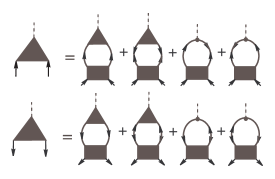
Figure 1: Dyson’s equations for the anomalous vertices. The shaded rectangle represents the pairing interaction.

$$\mathbf{\hat{T}}^{\left(1\right)}\left(\mathbf{n}\right)=\sum_{lm_{j}}\bm{\hat{\sigma}}\mathbf{b}_{lm_{j}}(\mathbf{n})\hat{g}\sum_{l^{\prime}}V_{ll^{\prime}}\frac{1}{2}\left\langle\mathcal{I}_{GG^{-}}\mathrm{Tr}\left[\hat{g}\left(\bm{\hat{\sigma}}\mathbf{b}_{l^{\prime}m_{j}}^{\ast}\right)\mathbf{\hat{T}}^{\left(1\right)}\right]\right.$$

$$\left.-\mathcal{I}_{FF}\mathrm{Tr}\left[\left(\bm{\hat{\sigma}}\mathbf{b}_{l^{\prime}m_{j}}^{\ast}\right)\left(\bm{\hat{\sigma}}\mathbf{\bar{b}}\right)\hat{g}\mathbf{\hat{T}}^{\left(2\right)}\left(\bm{\hat{\sigma}}\mathbf{\bar{b}}\right)\right]-\frac{\omega}{\Delta}\mathcal{I}_{FF}2i\left(\mathbf{b}_{l^{\prime}m_{j}}^{\ast}\mathbf{\times\bar{b}}\right)\right\rangle,$$ (23)

$$\mathbf{\hat{T}}^{\left(2\right)}\left(\mathbf{n}\right)=\sum_{lm_{j}}\hat{g}\bm{\hat{\sigma}}\mathbf{b}_{lm_{j}}^{\ast}(\mathbf{n})\sum_{l^{\prime}}V_{ll^{\prime}}\frac{1}{2}\left\langle\mathcal{I}_{G^{-}G}\mathrm{Tr}\left[\left(\bm{\hat{\sigma}}\mathbf{b}_{l^{\prime}m_{j}}\right)\hat{g}\mathbf{\hat{T}}^{\left(2\right)}\right]\right.$$

$$\left.-\mathcal{I}_{FF}\mathrm{Tr}\left[\left(\bm{\hat{\sigma}}\mathbf{b}_{l^{\prime}m_{j}}\right)\left(\bm{\hat{\sigma}}\mathbf{\bar{b}}\right)\mathbf{\hat{T}}^{\left(1\right)}\hat{g}\left(\bm{\hat{\sigma}}\mathbf{\bar{b}}\right)\right]-\frac{\omega}{\Delta}\mathcal{I}_{FF}2i\left(\mathbf{b}_{l^{\prime}m_{j}}\mathbf{\times\bar{b}}\right)\right\rangle.$$ (24)

Inspection of the equations reveals that the anomalous axial-vector vertices can be found in the following form

$$\mathbf{\hat{T}}^{\left(1\right)}\left(\mathbf{n},\omega\right)=\sum_{lm_{j}}\mathbf{B}_{l,m_{j}}\left(\omega\right)\left(\bm{\hat{\sigma}}\mathbf{b}_{l,m_{j}}\right)\hat{g},$$ (25)

$$\mathbf{\hat{T}}^{\left(2\right)}\left(\mathbf{n},\omega\right)=\sum_{lm_{j}}\mathbf{B}_{l,m_{j}}\left(\omega\right)\hat{g}\left(\bm{\hat{\sigma}}\mathbf{b}_{l,m_{j}}^{\ast}\right).$$ (26)

As explained above we are interested in solutions with $\mathbf{q}=0$. Then inserting of these forms into Eqs. (23), (24) allows to obtain the equations for $\mathbf{B}_{l,m_{j}}\left(\omega\right)$. We write the result in the matrix form (For brevity we omit the dependence on $\mathbf{n}$ and $\omega$)

$$\left(\begin{array}[]{c}\mathbf{B}_{1,m_{j}}\\ \mathbf{B}_{3,m_{j}}\end{array}\right)=-\left(\begin{array}[]{cc}V_{11}&-V_{13}\\ -V_{13}&V_{33}\end{array}\right)\left\{\left(\begin{array}[]{c}\sum_{l}\left\langle\left(A+\frac{\omega^{2}}{2\Delta^{2}}\mathcal{I}_{0}\right)\left(\mathbf{b}_{1,m_{j}}^{\ast}\mathbf{b}_{l,m_{j}}\right)\right\rangle\mathbf{B}_{l,m_{j}}\\ \sum_{l}\left\langle\left(A+\frac{\omega^{2}}{2\Delta^{2}}\mathcal{I}_{0}\right)\left(\mathbf{b}_{3,m_{j}}^{\ast}\mathbf{b}_{l,m_{j}}\right)\right\rangle\mathbf{B}_{l,m_{j}}\end{array}\right)\right.$$ (33)

$$\left.-2\left(\begin{array}[]{c}\sum_{l}\left\langle\mathcal{I}_{0}\left(\mathbf{\bar{b}b}_{1,m_{j}}^{\ast}\right)\left(\mathbf{\bar{b}b}_{l,m_{j}}\right)\right\rangle\mathbf{B}_{l,m_{j}}\\ \sum_{l}\left\langle\mathcal{I}_{0}\left(\mathbf{\bar{b}b}_{3,m_{j}}^{\ast}\right)\left(\mathbf{\bar{b}b}_{l,m_{j}}\right)\right\rangle\mathbf{B}_{l,m_{j}}\end{array}\right)+\frac{\omega}{\Delta}i\left(\begin{array}[]{c}\left\langle\mathcal{I}_{0}\left(\mathbf{b}_{1,m_{j}}^{\ast}\mathbf{\times\bar{b}}\right)\right\rangle\\ \left\langle\mathcal{I}_{0}\left(\mathbf{b}_{3,m_{j}}^{\ast}\mathbf{\times\bar{b}}\right)\right\rangle\end{array}\right)\right\}.$$ (38)

In this equation, the interaction matrix can be diagonalized by the unitary transformation (19). Further simplification is possible due to the fact that by virtue of Eqs. (21), (22) the coupling constants $W_{\pm}$ can be removed out of the equations. Explicit evaluation of equations obtained in this way for arbitrary values of $\omega$ and $T$ requires numerical computation. However, we can get a clear idea of the behavior of the vertex functions using the angle-averaged energy gap $\Delta^{2}\bar{b}^{2}\rightarrow\left\langle\Delta^{2}\bar{b}^{2}\right\rangle=\Delta^{2}$ in the quasiparticle energy $E_{\mathbf{p}}$. In this approximation, the functions $\mathcal{I}\left(\omega,T\right)$ and $A\left(T\right)$ can be moved beyond the angle integrals. Performing trivial integrations we then get a set of linear equations (two equations for each value of $m_{j})$. It is convenient to denote

$$\beta_{l,l^{\prime}}^{\left(m_{j}\right)}\equiv\left\langle\left(\mathbf{b}_{l,m_{j}}\mathbf{\bar{b}}\right)\left(\mathbf{b}_{l^{\prime},m_{j}}^{\ast}\mathbf{\bar{b}}\right)\right\rangle,$$ (39)

and

$$\Omega=\frac{\omega}{2\Delta}.$$ (40)

Then the set of equations can be written in the form

$$\mathbf{B}_{1,m_{j}}\left[\sqrt{V_{+}}\left(\Omega^{2}-\beta_{1,1}^{\left(m_{j}\right)}\right)-\sqrt{V_{-}}\beta_{1,3}^{\left(m_{j}\right)}\right]$$

$$+\mathbf{B}_{3,m_{j}}\left[\sqrt{V_{-}}\left(\Omega^{2}-\beta_{3,3}^{\left(m_{j}\right)}\right)-\sqrt{V_{+}}\beta_{3,1}^{\left(m_{j}\right)}\right]$$

$$=-i\Omega\left(\sqrt{V_{+}}\left\langle\mathbf{b}_{1,m_{j}}^{\ast}\times\mathbf{\bar{b}}\right\rangle+\sqrt{V_{-}}\left\langle\mathbf{b}_{3,m_{j}}^{\ast}\times\mathbf{\bar{b}}\right\rangle\right),$$ (41)

$$\mathbf{B}_{1,m_{j}}\left[-\sqrt{V_{-}}\left(\Omega^{2}-\beta_{1,1}^{\left(m_{j}\right)}\right)-\sqrt{V_{+}}\beta_{1,3}^{\left(m_{j}\right)}\right]$$

$$+\mathbf{B}_{3,m_{j}}\left[\sqrt{V_{+}}\left(\Omega^{2}-\beta_{3,3}^{\left(m_{j}\right)}\right)+\sqrt{V_{-}}\beta_{3,1}^{\left(m_{j}\right)}\right]$$

$$=-i\Omega\left(-\sqrt{V_{-}}\left\langle\mathbf{b}_{1,m_{j}}^{\ast}\times\mathbf{\bar{b}}\right\rangle+\sqrt{V_{+}}\left\langle\mathbf{b}_{3,m_{j}}^{\ast}\times\mathbf{\bar{b}}\right\rangle\right),$$ (42)

which can be solved to give

$$\mathbf{B}_{1,m_{j}}=\frac{-i\Omega}{\chi}\left[\left(\Omega^{2}-\beta_{3,3}^{\left(m_{j}\right)}\right)\left\langle\mathbf{b}_{1,m_{j}}^{\ast}\times\mathbf{\bar{b}}\right\rangle+\beta_{3,1}^{\left(m_{j}\right)}\left\langle\mathbf{b}_{3,m_{j}}^{\ast}\times\mathbf{\bar{b}}\right\rangle\right],$$ (43)

$$\mathbf{B}_{3,m_{j}}=\frac{-i\Omega}{\chi}\left[\left(\Omega^{2}-\beta_{1,1}^{\left(m_{j}\right)}\right)\left\langle\mathbf{b}_{3,m_{j}}^{\ast}\times\mathbf{\bar{b}}\right\rangle+\beta_{1,3}^{\left(m_{j}\right)}\left\langle\mathbf{b}_{1,m_{j}}^{\ast}\times\mathbf{\bar{b}}\right\rangle\right]~{}$$ (44)

with

$$\chi\left(\Omega\right)\equiv\Omega^{4}-\Omega^{2}\left(\beta_{1,1}^{\left(m_{j}\right)}+\beta_{3,3}^{\left(m_{j}\right)}\right)+\beta_{1,1}^{\left(m_{j}\right)}\beta_{3,3}^{\left(m_{j}\right)}-\beta_{1,3}^{\left(m_{j}\right)}\beta_{3,1}^{\left(m_{j}\right)}.$$ (45)

As is well known, poles of the vertex function correspond to collective eigen-modes of the system. Eigen- frequencies, $\Omega=\Omega^{\left(m_{j}\right)}$, of such oscillations satisfy the equation $\chi\left(\Omega^{\left(m_{j}\right)}\right)=0$. This equation gives

$$\left(\Omega_{\pm}^{\left(m_{j}\right)}\right)^{2}=\frac{1}{2}\left(\beta_{1,1}^{\left(m_{j}\right)}+\beta_{3,3}^{\left(m_{j}\right)}\pm\sqrt{\left(\beta_{1,1}^{\left(m_{j}\right)}-\beta_{3,3}^{\left(m_{j}\right)}\right)^{2}+4\beta_{1,3}^{\left(m_{j}\right)}\beta_{3,1}^{\left(m_{j}\right)}}\right).\allowbreak$$ (46)

Notice that the interaction parameters,$V_{\pm}$, drop out of the above solutions, which depend explicitly only on the partial gap amplitudes. This means that the contribution of excited bound pairs with $l=3$ into the spin oscillations is caused basically by spin-orbit interactions but not by the tensor forces.

Indeed, in Eqs. (43) - (46), the equilibrium order parameter is specified solely by means of the real vector $\mathbf{\bar{b}}$. If we switch off the interaction in the ${}^{3}F_{2}$ and ${}^{3}P_{2}-$${}^{3}F_{2}$ channels and consider pure ${}^{3}P_{2}$ pairing with $m_{j}=0$ we are then left with $\mathbf{\bar{b}=b}_{1,0}$ and $\Delta=\Delta_{1,0}$.  In this case, in Eqs. (43), (44), one has:

$$\int\frac{d\varphi}{2\pi}\left(\mathbf{b}_{1,m_{j}}^{\ast}\times\mathbf{\bar{b}}\right)=\int\frac{d\varphi}{2\pi}\left(\mathbf{b}_{3,m_{j}}^{\ast}\times\mathbf{\bar{b}}\right)=0~{}~{}\mathsf{for}~{}~{}m_{j}=0,\pm 2,$$ (47)

and the non-trivial solutions exist only for $m_{j}=\pm 1$. The explicit form of $\mathbf{b}_{l,m_{j}}$ can be obtained from Eq. (2):

$$\mathbf{b}_{1,0}=\sqrt{\frac{1}{2}}\left(\begin{array}[]{c}-n_{1}\\ -n_{2}\\ 2n_{3}\end{array}\right)\,,~{}\mathbf{b}_{1,1}=-\sqrt{\frac{3}{4}}\left(\begin{array}[]{c}n_{3}\\ in_{3}\\ n_{1}+in_{2}\end{array}\right),$$ (48)

$$\mathbf{b}_{3,0}=\sqrt{\frac{3}{4}}\left(\begin{array}[]{c}n_{1}\left(1-5n_{3}^{2}\right)\\ n_{2}\left(1-5n_{3}^{2}\right)\\ n_{3}\left(3-5n_{3}^{2}\right)\end{array}\right)\,,~{}\mathbf{b}_{3,1}=\sqrt{\frac{1}{2}}\left(\begin{array}[]{c}n_{3}\left(1-5n_{1}\left(n_{1}+in_{2}\right)\right)\\ in_{3}\left(1+5in_{2}\left(n_{1}+in_{2}\right)\right)\\ \left(n_{1}+in_{2}\right)\left(1-5n_{3}^{2}\right)\end{array}\right).$$ (49)

Making use of these expressions in Eq. (39) we find

$$\beta_{1,1}^{\left(\pm 1\right)}=\frac{1}{20}~{},~{}\beta_{3,3}^{\left(\pm 1\right)}=\frac{29}{70}~{},~{}\beta_{1,3}^{\left(\pm 1\right)}=\beta_{3,1}^{\left(\pm 1\right)}=-\frac{1}{70}\sqrt{\frac{3}{2}}.$$ (50)

Inserting these values into Eq. (46) we find $4\beta_{1,3}^{\left(\pm 1\right)}\beta_{3,1}^{\left(\pm 1\right)}\ll\left(\beta_{3,3}^{\left(\pm 1\right)}-\beta_{1,1}^{\left(\pm 1\right)}\right)^{2}$. By neglecting the small term $4\beta_{1,3}^{\left(\pm 1\right)}\beta_{3,1}^{\left(\pm 1\right)}$ under the root in Eq. (46) we obtain two (twofold) eigen-frequencies of spin oscillations in the condensate with $m_{j}=\pm 1$:

$$\omega_{-}^{\left(m_{j}\right)}~{}\simeq 2\Delta\sqrt{\beta_{1,1}^{\left(\pm 1\right)}}=\frac{1}{\sqrt{5}}\Delta,$$ (51)

$$\omega_{+}^{\left(m_{j}\right)}\simeq 2\Delta\sqrt{\beta_{3,3}^{\left(\pm 1\right)}}=\sqrt{\allowbreak\frac{58}{35}}\Delta.$$ (52)

In Refs. [9, 10], eigen-modes of spin oscillations in the ${}^{3}P_{2}$ superfluid neutron liquid was studied in a simple model restricted to excitations of the condensate with $l=1$. The spin wave energy (at $\mathbf{q}=0$) was found to be $\omega_{m_{j}}=\Delta/\sqrt{5}$. Equations (46), (51), (52) show that extending of the decomposition up to $l=1,3$ in Eqs. (25), (26) leads to a very small frequency shift of the known mode, $\omega=\omega_{-}^{\left(m_{j}\right)}\simeq\omega_{m_{j}}$, but opens the new additional mode of spin oscillations with $\omega=\omega_{+}^{\left(m_{j}\right)}$.

Neutrino decays of spin waves can play an important role in the cooling scenario of neutron stars. A simple estimate made in Ref. [10] has shown that the decays of spin waves with $\omega_{m_{j}}=\Delta/\sqrt{5}~{}$can become the dominant cooling mechanism in a wide range of low temperatures and modify the cooling trajectory of neutron stars. As well as the first mode, the second mode of spin oscillations is kinematically able to decay into neutrino pair. Therefore let us examine the wave excitation energies more accurately with taking into account the tensor forces. We will again focus on the condensation with $m_{j}=0~{}$by assuming $\Delta^{2}=\Delta_{1,0}^{2}+\Delta_{3,0}^{2}$, and

$$\mathbf{\bar{b}}\left(\mathbf{n}\right)=\frac{\Delta_{1,0}}{\Delta}\mathbf{b}_{1,0}\left(\mathbf{n}\right)+\frac{\Delta_{3,0}}{\Delta}\mathbf{b}_{3,0}\left(\mathbf{n}\right).$$ (53)

In this case Eqs. (47) are still valid and the non-trivial solutions to Eqs. (43), (44) exist only for $m_{j}=\pm 1$. Insertion of the expression (53) into Eq. (39) results in

$$\beta_{1,1}^{\left(\pm 1\right)} = \frac{1}{20}\frac{\Delta_{1}^{2}}{\Delta^{2}}\left(1-\frac{2}{7}\sqrt{6}\frac{\Delta_{3}}{\Delta_{1}}+\frac{58\Delta_{3}^{2}}{7\Delta_{1}^{2}}\right),$$

$$\beta_{3,3}^{\left(\pm 1\right)} = \frac{29}{70}\frac{\Delta_{1}^{2}}{\Delta^{2}}\left(1-\frac{32}{87}\sqrt{6}\frac{\Delta_{3}}{\Delta_{1}}+\frac{28}{87}\frac{\Delta_{3}^{2}}{\Delta_{1}^{2}}\right),$$

$$\beta_{1,3}^{\left(\pm 1\right)} = \beta_{3,1}^{\left(\pm 1\right)}=-\frac{1}{140}\sqrt{6}\frac{\Delta_{1}^{2}}{\Delta^{2}}\left(1-11\sqrt{6}\frac{\Delta_{3}}{\Delta_{1}}+\frac{32}{3}\frac{\Delta_{3}^{2}}{\Delta_{1}^{2}}\right).$$ (54)

Because $\beta_{l,l^{\prime}}^{\left(1\right)}=\beta_{l,l^{\prime}}^{\left(-1\right)}\equiv\beta_{l,l^{\prime}}$ we further omit the superscript $m_{j}=\pm 1$ by assuming that all the frequencies are twofold. Making use of Eqs. (54) we find

$$\omega_{-}^{2} =\Delta_{1,0}^{2}\left(\frac{13}{14}-\frac{1}{3}\sqrt{6}\frac{\Delta_{3}}{\Delta_{1}}+\frac{23}{21}\frac{\Delta_{3}^{2}}{\Delta_{1}^{2}}\right.$$

$$\left.-\sqrt{\frac{15}{28}-\frac{25}{49}\sqrt{6}\frac{\Delta_{3}}{\Delta_{1}}+\frac{485}{147}\frac{\Delta_{3}^{2}}{\Delta_{1}^{2}}-\allowbreak\frac{370}{441}\sqrt{6}\frac{\Delta_{3}^{3}}{\Delta_{1}^{3}}+\frac{55}{63}\frac{\Delta_{3}^{4}}{\Delta_{1}^{4}}}\right),$$ (55)

$$\omega_{+}^{2} =\Delta_{1,0}^{2}\left(\frac{13}{14}-\frac{1}{3}\sqrt{6}\frac{\Delta_{3}}{\Delta_{1}}+\frac{23}{21}\frac{\Delta_{3}^{2}}{\Delta_{1}^{2}}\right.$$

$$\left.+\sqrt{\frac{15}{28}-\frac{25}{49}\sqrt{6}\frac{\Delta_{3}}{\Delta_{1}}+\frac{485}{147}\frac{\Delta_{3}^{2}}{\Delta_{1}^{2}}-\allowbreak\frac{370}{441}\sqrt{6}\frac{\Delta_{3}^{3}}{\Delta_{1}^{3}}+\frac{55}{63}\frac{\Delta_{3}^{4}}{\Delta_{1}^{4}}}\right).$$ (56)

In Fig. 2, the energy of the collective spin excitations (at $\mathbf{q}=0$) is shown vs the ratio of the partial gaps $x=\Delta_{3,0}/\Delta_{1,0}$.

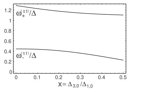
Figure 2: The energy gaps for the collective spin excitations $\omega_{-}^{\left(m_{j}\right)}$ and $\omega_{+}^{\left(m_{j}\right)}$ vs the ratio of partial gap amplitudes in the ${}^{3}F_{2}$ and ${}^{3}P_{2}$ channels. The energy gap of a neutron quasiparticle is given by $\Delta^{2}=\Delta_{1,0}^{2}+\Delta_{3,0}^{2}$.

According calculations of different authors, at the Fermi surface one has $\Delta_{3}\simeq 0.17\Delta_{1}$ (see, e.g., Ref. [20]). In this case our theoretical analysis predicts two degenerate modes with $\omega=\omega_{-}=0.42\Delta$, and two degenerate modes with $\omega=\omega_{+}=1.\,\allowbreak 19\Delta$.

Because of a rather small excitation energy the decay of the corresponding collective spin excitations into neutrino pairs should lead to an extension of the low-temperature domain where the volume neutrino emission dominates the surface gamma radiation in the star cooling. This effect was already demonstrated in Ref. [10], where only the lowest branch of the collective spin excitations $\omega=\Delta/\sqrt{5}\simeq\omega_{-}$ has been taken into account. The neutrino emissivity caused by the decay of the new spin modes predicted in this paper will be considered elsewhere.

References

• [1] O. V. Maxwell, Astrophys. J. 231 (1979) 201.
• [2] D. Page, J. M. Lattimer, M. Prakash, A. W. Steiner, Astrophys. J. Supp. 155 (2004) 623.
• [3] D. Page, J. M. Lattimer, M. Prakash, A. W. Steiner, Astrophys. J. 707 (2009) 1131.
• [4] P. S. Shternin, D. G. Yakovlev, C. O. Heinke, W. C. G. Ho, D. J. Patnaude, Mon. Not. Roy. Astron. Soc. 412 (2011) L108.
• [5] D. Page, M. Prakash, J. M. Lattimer, A. W. Steiner, Phys. Rev. Lett. 106 (2011) 081101
• [6] D. G. Yakovlev, A. D. Kaminker, and K. P. Levenfish, Astron. Astrophys. 343 (1999) 650.
• [7] L. B. Leinson and A. Pérez, Phys. Lett. B 638 114 (2006).
• [8] L. B. Leinson, Phys. Rev. C 81, 025501 (2010).
• [9] L. B. Leinson, Phys. Lett. B 689 (2010) 60.
• [10] L. B. Leinson, Phys. Rev. C 82, 065503 (2010).
• [11] K. Maki and H. Ebisawa, J.Low Temp. Phys. 15 (1974) 213.
• [12] R. Combescot, Phys. Rev. A 10 (1974) 1700.
• [13] R. Combescot, Phys. Rev. Lett. 33 (1974) 946.
• [14] P. Wölfe, Phys. Rev. Lett. 37 (1976) 1279.
• [15] P. Wölfe, Physica B 90 (1977) 96.
• [16] R. Tamagaki, Prog. Theor. Phys. 44 (1970) 905.
• [17] T. Takatsuka, Prog. Theor. Phys. 48 (1972) 1517.
• [18] A. A. Abrikosov, L. P. Gorkov, I. E. Dzyaloshinkski, Methods of quantum field theory in statistical physics, (Dover, New York, 1975).
• [19] A. B. Migdal, Theory of Finite Fermi Systems and Applications to Atomic Nuclei  (Interscience, London, 1967).
• [20] V. V. Khodel, V. A. Khodel, and J. W. Clark, Nucl. Phys. A 679 (2001) 827.
• [21] M. Baldo, J. Cugnon, A. Lejeune and U. Lombardo, Nucl. Phys. A 536 (1992) 349.
• [22] Ø. Elgarøy, L. Engvik, M. Hjorth-Jensen, E. Osnes, Nucl. Phys. A 607 (1996) 425.
• [23] M.V. Zverev, J. W. Clark, and V. A. Khodel, Nucl. Phys. A 720 (2003) 20.
• [24] A. Schwenk and B. Friman, Phys. Rev. Lett. 92, C82501 (2004).
• [25] A. J. Leggett, Phys. Rev. 140 (1965) 1869.
• [26] A. J. Leggett, Phys. Rev. 147 (1966) 119.
• [27] A. I. Larkin and A. B. Migdal, Zh. Experim. i Teor. Fiz. 44 (1963) 1703 [Sov. Phys. JETP 17 (1963) 1146].