Wavelength calibration for OSIRIS/GTC tunable filters

Abstract

OSIRIS (Optical System for Imaging and low Resolution Integrated Spectroscopy) is the first light instrument of the Gran Telescopio Canarias (GTC). It provides a flexible and competitive tunable filter (TF). Since it is based on a Fabry-Perot interferometer working in collimated beam, the TF transmission wavelength depends on the position of the target with respect to the optical axis. This effect is non-negligible and must be accounted for in the data reduction. Our paper establishes a wavelength calibration for OSIRIS TF with the accuracy required for spectrophotometric measurements using the full field of view (FOV) of the instrument. The variation of the transmission wavelength $\lambda(R)$ across the FOV is well described by $\lambda(R)=\lambda(0)/\sqrt{1+\left(R/f_{2}\right)^{2}}$, where $\lambda(0)$ is the central wavelength, $R$ represents the physical distance from the optical axis, and $f_{2}=185.70\pm 0.17\,$mm is the effective focal length of the camera lens. This new empirical calibration yields an accuracy better than $1$ Å across the entire OSIRIS FOV ($\sim$8′$\times$8′), provided that the position of the optical axis is known within 45 $\mu$m ($\equiv$ 1.5 binned pixels). We suggest a calibration protocol to grant such precision over long periods, upon re-alignment of OSIRIS optics, and in different wavelength ranges. This calibration differs from the calibration in OSIRIS manual which, nonetheless, provides an accuracy $\lesssim 1$Å  for $R\lesssim 2\arcmin$.

1 Introduction

Tunable filter (TF) instruments are becoming standard tools for mapping physical properties in extended astronomical sources. Most modern large telescopes have TFs based on Fabry-Perot interferometers (FPI; or etalons) such as the 11 m Southern African Large Telescope (SALT; Rangwala et al. 2008) or the Magellan-Baade 6.5 m telescope (Veilleux et al. 2010). The tunable imaging era began with the instrument of Atherton & Reay (1981) and many others have further developed the technique (Bland & Tully 1989; Brown et al. 1994). The current instrumental design is mainly based on the Taurus Tunable Filter (Bland-Hawthorn & Jones 1998) formerly mounted at the Anglo-Australian Telescope and afterward moved to the William Herschel Telescope at La Palma. The power of these instruments to perform spectrophotometric studies is clear. They allow for spectrophotometry with an unlimited number of wavelengths that can be scanned within a wavelength range. These etalon based TFs provide a central monochromatic field (MF). Outside the MF, and due to the use of etalons in collimated beam, there is a significant shift of wavelength that depends on the distance to the center. The instruments are designed to provide the largest possible MF, the wider possible wavelength range, and the narrower possible transmission band-pass. Besides, a proper calibration corrects the wavelength displacement with radius, thus recovering much of the field outside the MF to be used as an extended MF.

Among the large facilities hosting such instruments is the 10 m Gran Telescopio Canarias (GTC), located at the Roque de los Muchachos Observatory, that started its operations in the first semester of 2009 with OSIRIS (Cepa et al. 2005; Cepa 2010) as the first light instrument. OSIRIS stands for ”Optical System for Imaging and low Resolution Integrated Spectroscopy”. Besides conventional imaging and spectroscopy, it provides the additional capability of a TF observing mode working in the visible. It covers the wavelength range 0.365-1.0 $\mu$m with a nominal FOV of 7.8′$\times 8.5$′. Further commissioning tests establish the real un-vignetted FOV as $7.8\arcmin\times 7.8\arcmin$ (see OSIRIS commissioning webpage). OSIRIS specifications are extensively described in the manual provided by the instrument team (OSIRIS TF user manual – this document is referred to along the paper as OSIRIS manual). In particular, it provides the wavelength calibration procedure for radii outside the MF.

The OSIRIS FPI is an ideal instrument to map emission line regions in galaxies. It provides a high throughput with narrow transmission bandpass. The central wavelength is adjustable to account for the galaxy recession velocities, and the field of view (FOV) is reasonably large with a small pixel scale (0$\farcs$125). These properties together with the collecting power of a 10 m telescope, designed to get the best possible natural image quality, prompted us to design the Local Universe Survey (LUS), a research program optimized for OSIRIS. LUS aims at studying the star-formation history of a complete sample of nearby galaxies. We planned to obtain high signal-to-noise, high angular resolution, narrow band maps of all galaxies inside a volume of 3.5 Mpc radius. All irregulars and spirals inside a volume of 11 Mpc were also included, together with a sample of Virgo cluster galaxies. These observations suffice to produce a detailed unique description of the gaseous and stellar content of nearby galaxies. LUS has been defined within the ESTALLIDOS project in close collaboration with the Instituto Nacional de Astrofísica, Óptica y Electrónica in Mexico. Significant preparatory work was carried out in order to prove the feasibility of LUS; using the OSIRIS features described in the manual, we made simulations to estimate the exposure times, to choose precisely the filters (broad band and TF), and to optimize the observing procedure. Before submitting LUS as an ESO-GTC large program, we decided to test our simulations and procedures with real data.

The object selected to calibrate the photometric accuracy was M101, an extended and well-known nearby galaxy (7.38 Mpc, Rizzi et al. 2007), that exceeds the size of OSIRIS FOV. Observations were carried out to cover a large region of the southwestern part of the galaxy, containing also the well-known giant extragalactic H II  region NGC 5447. The central wavelengths of the TF were chosen to map emission lines such as H$\alpha$  or the sulphur doublet ([S II]$\lambda$$\lambda$6717, 6731), which allow to derive star-formation rates (SFRs) and electron densities of the star-forming regions. Even if not optimal, observations were made using the narrowest bandpass of FWHM 18 Å  available at the time. The precise central wavelength of the filter needed to separate [N II]$\lambda$6584  from H$\alpha$  was also tested, as distinguishing the two lines is critical to be able to use diagnostic diagrams like BPT (Baldwin et al. 1981). The basic data reduction was carried out using our own pipeline. Then, we reconstructed monochromatic emission line images taking into account the wavelength calibration provided in OSIRIS documentation. From this analysis, we found that H$\alpha$  fluxes and SFRs were globally consistent with values from the literature. However, the emission line ratios for both [N II]$\lambda$6584  over H$\alpha$ and the sulphur doublet ([S II]$\lambda$$\lambda$6717, 6731) were far from any observed value and whatever H II  region model. In an attempt to identify the problem, we started from scratch by using spectral calibration lamps to test wavelength shifts beyond the MF. The result of our calibration is the content of this paper. We have figured out that the prescriptions given in the manual suffice for the MF, while the new calibration in this paper allows for using OSIRIS in its full capability. It permits spectrophotometry in the full FOV with a wavelength accuracy as good as that in the MF. In our view OSIRIS is an extremely powerful instrument which could be seriously limited if only the MF can be used for spectrophotometry. Although our work was designed to recalibrate our fields and being able to recover reliable emission line fluxes over the entire OSIRIS FOV, it is of interest beyond the original scope, and may broaden the community of OSIRIS users.

The paper is organized as follows: in § 2 we introduce the basic optical concepts required to understand both the nature of the problem and the calibration procedure. § 3 shows how the original wavelength calibration needs refinement to provide an accuracy better than 1Å  in the full FOV. Based on the data introduced in § 4, the new calibration is worked out in § 5. In § 6 we recommend a wavelength calibration protocol that goes all the way from a detailed test of the long-term stability of the system, to a black-box recipe for urgent calibration. The conclusions of the work are summarized in § 7.

2 Basics of OSIRIS/GTC tunable filter optics

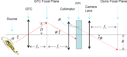
Figure 1: Schematic of the OSIRIS/GTC optical layout. A light beam, in red, crosses the system from left to right, finding the GTC telescope, the collimator, the Fabry-Perot interferometer, the camera, and OSIRIS focal plane. The different symbols are defined in the main text.

In essence, the optical layout of OSIRIS/GTC TFs is made of three lenses and a FPI, as sketched in Fig. 1. The first element, of effective focal length $f_{0}$, represents the telescope (GTC). Then a lens, of effective focal length $f_{1}$, collimates the light coming from the GTC focal plane, so that the FPI is illuminated in collimated beam. As represented in Fig. 1, a point in the focal plane of GTC, at a distance $D$ from the optical axis, enters the FPI interferometer with an angle $\theta$. Then

$$D=f_{1}\tan\theta=f_{0}\tan\alpha\simeq f_{0}\alpha,$$ (1)

where $\alpha$ represents the angular distance to the optical axis of the source on the sky. The wavelength transmitted by a FPI depends on the incidence angle as

$$\lambda(\theta)=\lambda(0)\cos\theta\,,$$ (2)

where $\lambda(0)$ is the central wavelength (e.g., Born & Wolf 1980; Beckers 1998; Veilleux et al. 2010). The final optical element, the camera, has an effective focal length $f_{2}$, so that,

$$R=f_{2}\tan\theta,$$ (3)

where $R$ is the position of the source on OSIRIS focal plane. Combining Eqs. (2) and (3), one gets the TF wavelength calibration equation in terms of the physical distance to the optical axis $R$. It is given by

$$\lambda(R)=\frac{\lambda(0)}{\sqrt{1+\left(\frac{R}{f_{2}}\right)^{2}}},$$ (4)

or equivalently, employing Eq. (1), it can be expressed in terms of the angular distance projected on the sky

$$\lambda(\alpha)=\frac{\lambda(0)}{\sqrt{1+\left(\alpha\,\frac{f_{0}}{f_{1}}\right)^{2}}}.$$ (5)

If $\alpha$ is small enough, then Eq. (5) can be expanded to first order giving rise to

$$\lambda(\alpha) \simeq \lambda(0)\,\big{(}1-C\,\alpha^{2}\big{)},$$ (6)

$$C = \frac{f_{0}^{2}}{2f_{1}^{2}},$$

and equivalently in terms of the physical distance

$$\lambda(R) \simeq \lambda(0)\,\big{(}1-C^{*}\,R^{2}\big{)},$$ (7)

$$C^{*} = \frac{1}{2f_{2}^{2}}.$$

The plate scale on OSIRIS focal plane relates the effective focal lengths of the three optical elements. Combining Eqs. (1) and (3), the plate scale $S$ turns out to be

$$S={d\alpha\over{dR}}={{f_{1}}\over{f_{0}f_{2}}},$$ (8)

which we use to link the two calibration constants,

$$C^{*}=C\,S^{2}.$$ (9)

OSIRIS manual employs Eq. (6) for wavelength calibration, therefore, it assumes the FOV to be small enough for the first order expansion to hold. In addition, the calibration is performed in angular coordinates on the sky, so that uncertainties in the plate scale affect the wavelength calibration. We propose using Eq. (4) instead. It makes the calibration sensitive only to the uncertainties of the focal length of the camera $f_{2}$, and it considers all the terms of the expansion. As we show in the next section, high order terms are needed to calibrate the field outside the MF.

Table 1: Summary of the basic optical parameters for OSIRIS/GTC wavelength calibration.

Physical Parameter	Symbol	Nominal Value	Best Estimate
GTC eff. focal length	$f_{0}$	170 m $[{\rm a}]$	165.3 $\pm$ 0.2 m $[{\rm h}]$
Collimator eff. focal length	$f_{1}$	1.240 m $[{\rm b}]$	1.275 $\pm$ 0.001 m $[{\rm i}]$
Camera eff. focal length	$f_{2}$	181 mm $[{\rm b,c}]$	185.70 $\pm$ 0.17 mm
Calibration constant	$C=f_{0}^{2}/(2\,f_{1}^{2})$	$7.9520\,\times\,10^{-4}$arcmin-2 $[{\rm d}]$	(7.517 $\pm$ 0.014)$\,\times\,10^{-4}$arcmin-2$[{\rm j}]$
Calibration constant	$C^{*}=1/(2\,f_{2}^{2})$	15.262 m-2	14.499 $\pm$ 0.027 m-2
		—	(3.2624 $\pm$ 0.0057) $\times\,10^{-9}$ pixel-2
OSIRIS pixel size (1$\times$1)		15 $\mu$m $[{\rm a,b,c,d}]$	—
OSIRIS pixel size (2$\times$2)		30 $\mu$m	—
OSIRIS plate scale (1$\times$1)	$S=f_{1}/(f_{0}f_{2})$	0$\farcs$125 pixel-1 $[{\rm a,b,d,e}]$	0$\farcs$127 pixel-1 $[{\rm k}]$
OSIRIS plate scale (2$\times$2)		0$\farcs$250 pixel-1	—
OSIRIS/GTC eff. focal length	$f_{0}f_{2}/f_{1}$	24.752 m $[{\rm b,g}]$	—
OSIRIS center position (2$\times$2)	(xc1, yc1)	(1059$\pm$ 2, 983$\pm$ 2) $[{\rm f}]$	(1053.6 $\pm$ 2.2,979.5 $\pm$ 1.8)
	(xc2, yc2)	(-1$\pm$ 2, 981$\pm$ 2) $[{\rm f}]$	(-9.8 $\pm$ 2.7,975.8 $\pm$ 1.1)

3 Motivation for an updated calibration

Inconsistencies in emission line ratios prompted us to reconsider OSIRIS wavelength calibration (§ 1). The importance of this effect can be disclosed and quantified using monochromatic images of known wavelength, as those provided by the GTC wavelength calibration unit. When the instrument is illuminated with a monochromatic beam of known wavelength $\lambda_{\rm line}$, the ring appearing in the focal plane traces where OSIRIS transmission matches $\lambda_{\rm line}$ (see Fig. 2). In principle, the position of the optical axis and the tuned central wavelength $\lambda(0)$ are given, therefore, one can easily measure the difference between the true wavelength $\lambda_{\rm line}$, and that provided by the nominal calibration in OSIRIS manual (Eq. (6)). If the ring is observed to have a radius $R$ (Fig. 2), then the error in wavelength is given by

$$\Delta\lambda=\lambda_{\rm line}-\lambda(R)=\lambda_{\rm line}-\lambda(0)\,\big{(}1-C\,S^{2}\,R^{2}\big{)},$$ (10)

where $C=7.9520\times 10^{-4}{\rm arcmin}^{-2}$ is the calibration constant appearing in the manual, and $S$ is the nominal plate scale ($0\farcs 125\,$ pixel^-1; see Table 1 with OSIRIS properties).

The black dots in Fig. 3 show $\Delta\lambda$ for a suite of 17 monochromatic images used for calibration (details are given in § 4). Note that the error in the true wavelength can be as large as 6 Å  at the FOV outskirts ($R\simeq 4$′; see Fig. 3). If rather than using the approximate Eq. (6), theoretical wavelengths are computed using the full Eq. (5), then one obtains the triangles in Fig. 3. The errors have been somewhat reduced, but they still remain as large as 4 Å  at 4′. Two main conclusions can be drawn from Fig. 3. First, the original calibration procedure does not provide correct wavelengths within 1 Å  when $R>2$′. Second, in order to achieve such an accuracy, one has to use the full Eq. (4) combined with a new calibration constant more precise than that inferred from the nominal values of the focals.

4 Data

Figure 3 and the calibration worked out in § 5 are based on a sample of 17 monochromatic images produced by arc lamps from the Instrument Calibration Module of GTC (ICM). They were obtained in two different runs and using the OSIRIS red arm. Their main properties are summarized in Table 2. The images were taken by the GTC staff who kindly provided them upon request. The OSIRIS FOV is imaged onto two CCDs that are separated by a gap. The distance between the CCDs is approximately 9$\farcs$2. The two OSIRIS science CCDs are of type E2V 44-82, back illuminated, with 2048 x 4096 pixels each when using a 1$\times$1 binning. OSIRIS was tuned to different central wavelengths in order to produce the characteristic ring for every monochromatic line (Fig. 2). They were obtained using the standard mode of operation with a binning 2$\times$2. The separation between any two consecutive orders of interference is called the free spectral range. In order to select the desired transmission order of the FP a blocking filter is required. The filters used in this study are also shown in Table 2.

In addition to the above monochromatic exposures, three images with strong sky emission rings were also requested in order to compare the wavelength calibration obtained from the ICM and from the sky. They are also listed in Table 2.

Table 2: Characteristics of the calibration data.

$\lambda(0)$	$\lambda_{\rm line}$	Species	TF FWHM	Blocking Filter	Observing
(Å)	(Å)		(Å)	(nm/nm)	Date
6598.9	6532.9	NeI	18	f657/35	10-02-2011
6630.0	6598.9	NeI	18	f657/35	10-02-2011
6650.0	6598.9	NeI	18	f657/35	10-02-2011
6950.0	6929.5	NeI	16	f694/44	03-03-2011
6975.0	6929.5	NeI	16	f694/44	03-03-2011
7000.0	6929.5	NeI	16	f694/44	03-03-2011
7020.0	6929.5	NeI	16	f694/44	03-03-2011
7050.0	7032.4	NeI	16	f694/44	03-03-2011
7070.0	7032.4	NeI	16	f709/45	03-03-2011
7090.0	7032.4	NeI	16	f709/45	03-03-2011
7100.0	7032.4	NeI	16	f709/45	03-03-2011
7120.0	7032.4	NeI	16	f709/45	03-03-2011
7650.0	7635.1	ArI	18	f770/50	03-03-2011
7680.0	7635.1	ArI	18	f770/50	03-03-2011
7700.0	7635.1	ArI	18	f770/50	03-03-2011
7720.0	7635.1	ArI	18	f770/50	03-03-2011
7740.0	7635.1	ArI	18	f770/50	03-03-2011
6900.0	6834.4-6841.9	telluric OH	12	f666/36	12-02-2011
6925.0	6871.0-6880.9	telluric OH	12	f666/36	12-02-2011
6950.0	6864.0-6871.0	telluric OH	12	f680/36	12-02-2011

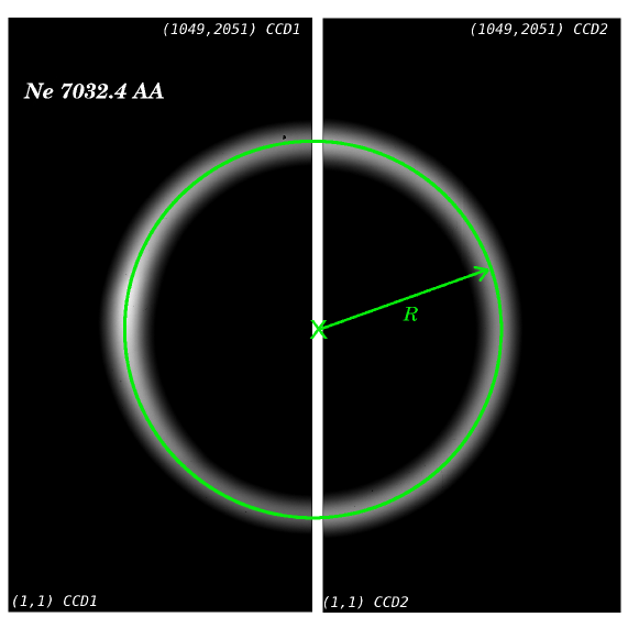
Figure 2: Image of a NeI spectral calibration lamp illuminating the OSIRIS detectors. It forms a ring which we have outlined with a green circle of radius $R$ centered at $X$. OSIRIS has been tuned to a central wavelength of 7070 Å, whereas the NeI emission occurs at 7032.4 Å. Binned coordinates (1,1) and (1049,2051) are also drawn on the image.

5 Wavelength calibration

As we argue in § 3, improving the original calibration demands both including all the terms neglected in the approximate Eq. (6) and determining the calibration constants directly from observations. We measured $C^{*}$ because it does not require knowing the plate scale $S$, therefore, we make the calibration insensitive to errors in $S$. Besides, $C$ follows directly from $C^{*}$ and $S$ via Eq. (9).

Calibrating an image is assigning a wavelength to each point of the FOV using Eq. (4). Three different unknowns must be set, namely, the position of the center, origin of distances, the calibration constant, and the central wavelength. This section describes a precise determination of the two first ingredients using the data described in § 4. The central wavelength is determined within 1 Å as part of the regular OSIRIS tuning protocol. This claim is confirmed in § 5.2 since it also affects the empirical determination of $C^{*}$. The three unknowns have uncertainties that determine the calibration accuracy. The propagation of these uncertainties into the final wavelength is studied in § 5.3.

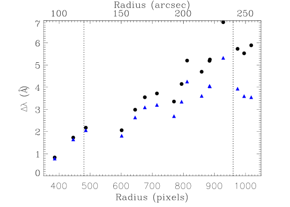
Figure 3: Differences between the true wavelengths and that derived using the nominal OSIRIS calibration procedure. Each point has been inferred from one image similar to that in Fig. 2. The discrepancies increase with distance from the optical axis $R$ ($\equiv Radius$). The black dots correspond to the nominal calibration based on the approximate Eq. (6), whereas the blue triangles used the full Eq. (5). Abscissas are given in pixels (bottom) and arcsec (top), the latter calculated using the nominal plate scale. Vertical dotted lines show the radius of the MF ($\sim$2′) and the non-vignetted FOV ($\sim$4′).

5.1 TF optical center

The nominal TF optical center is located in the pixel (2118, 1966) from the pixel (1,1) of CCD1, including the 50 pixels of overscan. Thus, assuming the nominal gap between the CCDs of 72 pixels, the center lies within the gap of the two CCDs (see Fig. 2). As pointed out before, our images have been taken with the standard 2$\times$2 binning. Therefore, we might expect a center positioned at binned pixels (1059,983) – see Table 1. Taking into account that the distance between the CCDs is $\sim$36 binned pixels, the TF optical center should be placed 1 pixel to the left of column 1 of CCD2.

We have measured the optical center for our calibration lamps using the following procedure: first we generate a grid of possible TF optical pixel centers ($x_{\rm trial}$,$y_{\rm trial}$) independently for both CCDs. Since the gap between CCDs is not constant (it varies from top to bottom due to both a rotation and a 2 pixels vertical shift of CCD2 with respect to CCD1), the solution of assuming independent centers bypasses the difficulty of knowing the relative position of the two CCDs. Then, for every trial position on each CCD, the calibration lamp image was divided in 8 regions of 45^∘ (4 in each CCD). Each region is azimuthally averaged and the distance of the ring to the assumed center is measured. Due to both possible irregularities in the optical system and the offset between the true and trial centers, the measurements of the ring radii for each region are not the same. We assign the best center from our grid of trial values looking for the value that, providing the same mean center within the errors for both CCDs, minimizes the scatter among the radii of the eight different sectors. If the monochromatic images were noiseless and the ring perfectly circular, our center-finding algorithm would provide the correct value. In practice, however, the procedure has some errors that we estimate by comparing centers obtained from different rings.

Figure 4 shows the best centers obtained for each calibration lamp image, and the mean value over our whole sample. They turn out to be

$$(x_{\rm c1},y_{\rm c1})=(1053.6\pm 2.2,979.5\pm 1.8),$$

for CCD1, and

$$(x_{\rm c2},y_{\rm c2})=(-9.8\pm 2.7,975.8\pm 1.1),$$ (11)

for CCD2, where each center refers to its own CCD. The error bars in Eq. (11) represent the standard deviation among the values obtained from the different rings, therefore, assuming the errors of the different measurements to be independent, the error bars of the average values should be scaled down by a factor of the order of the square root of the number of rings ($\sim$4, e.g., Martin 1971).

In the following we use the mean values as the centers for every calibration lamp. The nominal values of the centers are also included in Fig. 4 as triangles. The nominal center of CCD1 may be marginally in agreement with our empirical determination. However, the center of CCD2 is clearly inconsistent with its nominal value.

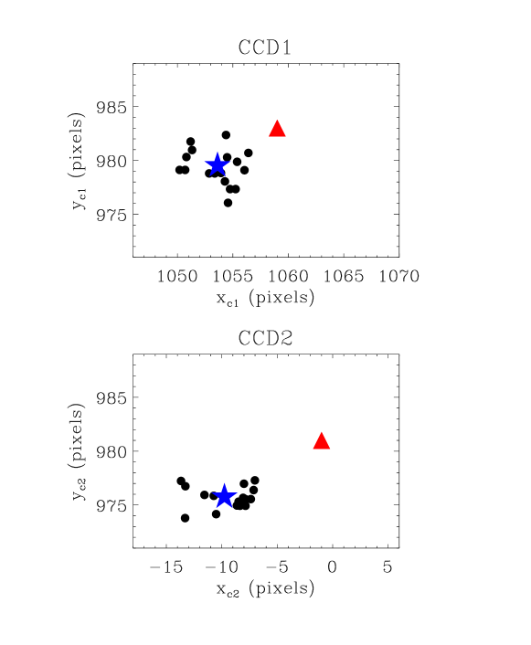
Figure 4: OSIRIS optical centers obtained using our sample of calibration lamps (black dots). The two CCDs are shown separately (CCD1, top; CCD2, bottom). The blue stars represent the average value of the centers, which we take as reference for all lamps. The red triangles show the nominal center positions. The limits of the plots correspond to the parameter space covered by the trial values used to determine the position of the centers. Positions are given in binned pixels on the chips. Abscissas larger than 1049 or negative imply centers outside the CCDs.

5.2 Calibration constants

A trivial manipulation of Eq. (4) renders

$$\Big{[}{{\lambda(0)}\over{\lambda(R)}}\Big{]}^{2}=1+f_{2}^{-2}\,R^{2},$$ (12)

thus, a straightforward linear regression allows us to derive the value of the effective focal length of the camera lens ($f_{2}$) given the positions on the image ($R$) of lines of known wavelength ($\lambda(R)=\lambda_{\rm line}$). Figure 5 shows the data and fit leading to the empirical determination of $f_{2}$. We have measured the distance from the center of the system (obtained in § 5.1) to the positions of the rings produced by the 17 different monochromatic images described in § 4. As it was done in the previous section, this distance was measured 8 times corresponding to the 8 different sectors in which each ring was divided. They are plotted in Fig. 5, showing a very small scatter that provides confidence on the procedure. The best value for $f_{2}$ was derived by fitting a straight line to the points in Fig. 5 using a standard linear least squares minimization routine. Once the slope is properly transformed assuming 1 binned pixel = 30 $\mu$m (Table 1), the best fit gives

$$f_{2}=185.70\pm 0.17~{}{\rm mm}.$$ (13)

The fit also provides the $y-$intercept. It turns out to be consistent with one ($0.99995\pm 0.00006$) supporting the use of Eq. (12) to represent the wavelength variation along OSIRIS FOV.

Note how the empirical $f_{2}$ differs from the nominal value of $181$ mm (Table 1). This difference in the effective focal length of the camera lens was not completely unexpected. From astrometry and laboratory tests we know that the actual plate scale of OSIRIS is $\sim$0$\farcs$127 pixel^-1 rather than the nominal 0$\farcs$125 pixel^-1 (Table 1). This difference can only be accounted for if the nominal focal lengths differ from the actual values (see Eq. (8)).

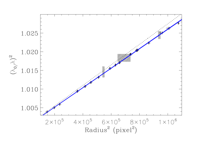
Figure 5: Fit used to derive empirically the value of the camera lens effective focal length ($f_{2}$). Black crosses represent the values measured using the calibration lamps, one for each region of every ring image. The blue line represents the best fit to our measurements. Hatched areas indicate the range of possible values for the three sky rings. The black dotted line shows the result to be expected using the nominal value for $f_{2}$, which is way off the observed values.

The hatched areas in Fig. 5 show the position of three rings from sky lines also measured in this work (§ 4). The measurements are not represented as points but as regions, since they are not single lines but series covering a fairly broad spectral range (Table 2). We have considered the wavelengths of the sky lines covered by each filter as an error in the ordinate axis. In the abscissa axis, the errors correspond to the position of the 8 different sectors in the image. It is worth pointing out that even if the chosen sky lines are not suitable to be used for wavelength calibration, their position on OSIRIS focal plane are fully consistent with the new calibration carried out in this work (Fig. 5).

Once $f_{2}$ has been obtained, and in order to compare with the nominal values, we have derived the calibration constants $C^{*}$ and $C$ using Eqs. (7) and (9),

$$C^{*}=14.499\pm 0.027{\rm~{}m}^{-2}=(3.2624\pm 0.0057)\times 10^{-9}\,{\rm pixel}^{-2},$$

$$C=(7.517\pm 0.014)\times 10^{-4}\,{\rm arcmin}^{-2}\,[S/0\farcs 125{\rm\,pixel}^{-1}]^{-2}.$$ (14)

$C$ uses $S=0\farcs 125$  pixel^-1 for the sake of comparison with the nominal values, although the wavelengths calibrated using $C$ in Eq. (5) are independent of the plate scale. The errors in $C$ and $C^{*}$ have been calculated by propagating the error of $f_{2}$ (Eq. (13)). In the same way, the ratio between the GTC and OSIRIS collimator effective focal lengths can be determined yielding $f_{1}/f_{0}=(7.5024\pm 0.0070)\times 10^{-3}$ with $S=0\farcs 125$  pixel^-1.

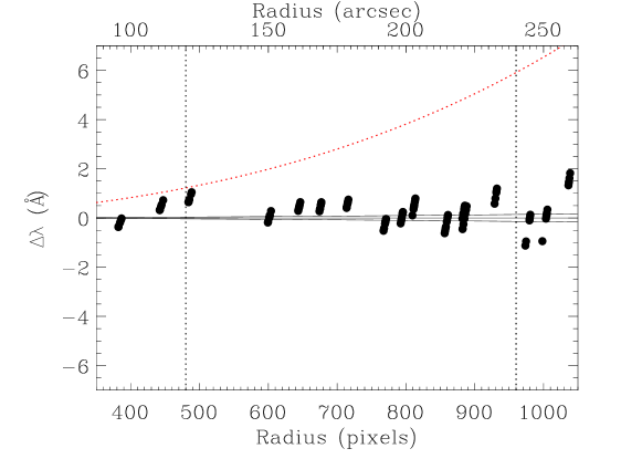
Figure 6: Wavelength difference in Å between the actual wavelength of the calibration lines and that predicted by the new calibration. Black dots represent the measurement for each ring sector of every calibration lamp. The black solid lines show the uncertainty caused by the error in $f_{2}$. The red dotted line indicates the deviation from the actual wavelength of the calibration lines given by nominal calibration. The scale on top has been calculated using the nominal plate scale. Vertical dotted lines show the radii of the MF ($\sim$2′) and the non-vignetted FOV ($\sim$4′)

Figure 6 represents the difference between the true wavelengths of the lines and that inferred using our calibration. It is equivalent to Fig. 3 but using the new calibration. The reason for including this figure is threefold. First, it shows how the systematic trend present in Fig. 3 has disappeared, meaning that the new calibration holds throughout the whole OSIRIS FOV. Second, the observed scatter provides an upper limit to the error in tuning the central wavelength of OSIRIS. As one can see from Table 2, all but one of the monochromatic images were taken with a different $\lambda(0)$. Any random error existing in setting $\lambda(0)$ would be transferred to $\Delta\lambda$ as a random fluctuation of amplitude similar to that of $\lambda(0)$ (see Eq. (10)). The scatter in Fig. 6 does not exceed 1Å, and so does the setting of $\lambda(0)$. Finally, Fig. 6 also shows $\Delta\lambda$ considering the original calibration (the red dotted line). The error remains within the acceptable limit of $\Delta\lambda<1~{}$Å when $R<2$′, which approximately coincides with OSIRIS MF.

5.3 Error budget

Three main sources of uncertainty burden the wavelength calibration, namely, errors in the central wavelength $\delta\lambda(0)$, errors in the calibration constant $\delta C^{*}$, and errors in the center position $\delta x_{\rm c}$, and $\delta y_{\rm c}$. The error in the central wavelength has not been explicitly treated before but, according to the arguments given in the previous section, it is within the nominal 1 Å  set by the procedure to tune OSIRIS (see OSIRIS manual).

Using Eq. (4), it is possible to propagate these errors onto the wavelength calibration $\delta\lambda(R)$. The result of this exercise turns out to be

$$\frac{\delta\lambda(R)}{\lambda(R)}=\frac{\delta\lambda(0)}{\lambda(0)},$$ (15)

for the central wavelength error $\delta\lambda(0)$,

$$\frac{\delta\lambda(R)}{\lambda(R)}=\frac{-\delta C^{*}}{2\,C^{*}}\,\left[1-\frac{\lambda^{2}(R)}{\lambda^{2}(0)}\right],$$ (16)

for the calibration constant error $\delta C^{*}$, and finally,

$$\frac{\delta\lambda(R)}{\lambda(R)}=\frac{\delta x_{\rm c}\cos\phi}{R}\,\left[1-\frac{\lambda^{2}(R)}{\lambda^{2}(0)}\right],$$ (17)

for the error of the center in the $x$-axis ($\delta x_{\rm c}$). The variable $\phi$ stands for the azimuth of the point relative to the center, and it has been introduced for convenience since using $|\cos\phi|=1$ in Eq. (17) grants an upper limit to $\delta\lambda$. The error due to uncertainties in the vertical direction is formally identical to that for the horizontal direction replacing $\delta x_{\rm c}\cos\phi$ with $\delta y_{\rm c}\sin\phi$.

In order to illustrate the relative importance of the various sources of error, Fig. 7 shows the typical $\delta\lambda(R)$ to be expected with our calibration, assuming the central wavelength to be tuned to H$\alpha$ (6563 Å). The dotted line corresponds to the effect of 1Å  uncertainty in the determination of the central wavelength. It sets a minimum threshold to the calibration error in the full OSIRIS FOV. The dashed line considers $\delta C^{*}=0.027$ m^-2, which corresponds to the error in $f_{2}$ derived in our calibration (see § 5 and Table 1). The calibration constant seems to be precise enough and does not limit the wavelength calibration. Finally, the solid line corresponds to a center uncertainty given by $\delta x_{\rm c}\,\cos\phi=3$ pixels. It produces an error in the wavelength scale that is almost 2 Å in the outer parts of the FOV, exceeding the threshold set by the central wavelength. Three pixels represent a significant overestimate of the uncertainties we expect for the centers; if we consider a more realistic $\delta x_{c}\,\cos\phi\leq 1.5$ pixels, then $\delta\lambda(R)\leq 1$Å, and the error in the center position does not limit the calibration. We use this overestimated value to illustrate that the precision in the center turns out to be the critical point of the wavelength calibration.

Figure 7: Wavelength errors in the calibration ($\delta\lambda$) as a function of the distance to the center of the FOV. As indicated in the inset, the curves represent a mis-tuning of the central wavelength ($\delta\lambda(0)\not=0$, dotted line), errors in calibration constant ($\delta C^{*}\not=0$, dashed line), and uncertainties locating the center of the FOV ($\delta x_{c}\not=0$, solid line). The errors we consider are realistic, except perhaps for an overestimate of $\delta x_{c}$ (see main text). The central wavelength was assumed to be tuned to H$\alpha$. Vertical dotted lines show the radius of the MF ($\sim$2′) and the non-vignetted FOV ($\sim$4′).

The question arises as to whether $\delta\lambda(R)\leq 1\,$Å suffices to compute the line fluxes that triggered our work (§ 1). We address the problem assuming the TF bandpass to behave as expected (e.g., Born & Wolf 1980; Beckers 1998),

$$\tau=\left[1+\left[\frac{2\,\left(\lambda_{s}-\lambda(R)\right)}{\sigma_{\lambda}}\right]^{2}\right]^{-1},$$ (18)

with $\sigma_{\lambda}$ the FWHM of the TF transmission bandpass, and $\lambda(R)$ the wavelength calibrated above. Consider a spectral line of wavelength $\lambda_{s}$ and integrated flux $F$. Then, the flux measured in a given point of the focal plane $R$, $F_{m}(R)$, turns out to be

$$F_{m}(R)=\tau\,F,$$ (19)

where we have assumed the line to be much narrower than the TF transmission (as it is indeed the case for the emission lines in typical H II  regions). Equation (19) provides the recipe to retrieve the true flux from the observed one knowing the transmission. If $\lambda(R)$ is uncertain then $\tau$ is uncertain as well, producing the error on $F$ that we try to evaluate. The error in the retrieved flux $\delta F$ due to the error in the central wavelength $\delta\lambda(R)$ was derived by applying the law of propagation of errors (e.g., Martin 1971) to Eq. (19), and it is given by

$$\frac{\delta F}{F}\simeq-\frac{d\ln\tau}{d\lambda(R)}\delta\lambda(R).$$ (20)

After some trivial manipulations, the previous equation becomes

$$\frac{\delta F}{F}\simeq-4\,\big{[}(1-\tau)\,\tau\big{]}^{1/2}\,\frac{\delta\lambda(R)}{\sigma_{\lambda}}.$$ (21)

Since $0\leq\tau\leq 1$, then $\big{[}(1-\tau)\,\tau\big{]}^{1/2}\leq 0.5$, and so

$$\Big{|}\frac{\delta F}{F}\Big{|}\leq 2\Big{|}\frac{\delta\lambda(R)}{\sigma_{\lambda}}\Big{|}.$$ (22)

For $\delta\lambda(R)\leq 1\,$Å  and a TF FWHM of $\sigma_{\lambda}\simeq 20$ Å, Eq. (22) yields $|\delta F/F|\leq 0.1$. This error is small enough for most applications, including those mentioned in § 1 – e.g., it provides SFRs within 10 % using the customary recipes (e.g., Kennicutt 1998), and it is much smaller than the intrinsic scatter of the sulphur doublet ([SII]$\lambda\lambda$6717, 6731) used to determine electron densities (e.g., Bresolin & Kennicutt 2002). Three final comments are in order. First, a scaling factor $\tau$ does not affect our error estimate, which is the reason why the peak transmission in Eq. (18) was set to one. Second, Eq. (19) implicitly assumes the observed spectrum to have no continuum. If there is continuum, then the arguments remain valid replacing $F_{m}(R)$ with the difference between the fluxes measured in line and in continuum. Finally, the upper limit in Eq. (22) significantly overestimates the true error when the wavelength setting is close to the peak transmission (see Eq. (21) with $\tau\simeq 1$).

6 Wavelength calibration protocol

Based in our previous experience, this section puts forward a set of guidelines to carry out an accurate wavelength calibration of the upcoming scientific data. It involves routine observations of calibration lamps together with the astronomical images. Since no extensive tests on the stability of the OSIRIS TF center and calibration constant have been performed yet, they are needed to ensure the accuracy presented in this work and to identify other possible errors. The protocol will also allow to study and quantify the wavelength dependence of the calibration parameters.

In general, the calibration process should consist of the following four steps:

1. Obtain a number of calibration lamp images during the observation run covering the full FOV. Preferably, select a monochromatic emission line from a lamp with a wavelength near to the scientific observation. Then, map its positions along the OSIRIS FOV by changing the central wavelength of the TF.

2. Calculate the center of the system using the rings corresponding to the monochromatic lines. Check that it is the same for all rings within a reasonable error (a few pixels; see Fig. 4).

3. Calculate the value of the effective focal length of the camera lens ($f_{2}$) by fitting linearly Eq. (12). This equation should be fitted in pixels or in a physical length (mm) to avoid crosstalk with errors in the plate scale.

4. Calibrate the scientific images by assigning the wavelength given by Eq. (4) to every pixel. Use the empirically derived $f_{2}$ and optical center.

We recommend to apply the calibration described here to each CCD independently, and before applying astrometric corrections to avoid other error sources. Eventually, if the instrument turns out to be stable, the calibration will consist only of step 4 with $f_{2}$ and the center derived in this paper.

For observations already in hand using the full OSIRIS FOV, we suggest to recalibrate the images using the prescriptions and constants given in this paper (Eqs. (4), (11), and (13)). Whenever a calibration ring is available as ancillary data, we recommend computing the center and compare its value with our estimate (Eq. (11)). A remainder is important: as we explained in §5.1, the trials for determining the best center have been carried out on the raw data. If the data to be re-calibrated have already been processed (e.g., overscan removed), then the values of the best center have to be shifted accordingly.

Existing observations using only OSIRIS MF do not need re-calibration. The approximate original prescriptions in OSIRIS manual suffice.

7 Conclusions

OSIRIS TF and GTC represent a unique combination to study the physical properties of extended astronomical sources. They are capable of providing high S/N, narrow band images, over a relatively large field with an excellent spatial sampling. The OSIRIS TF is based on a conventional FPI mounted in collimated beam. FPI based instruments provide an area of the FOV, the MF, where the wavelength can be considered constant within the band-pass of the TF. However, outside the MF there is a significant shift in wavelength which depends on the distance to the optical axis. Therefore, in order to benefit from OSIRIS large FOV, an accurate wavelength calibration is needed.

Motivated by inconsistencies in the measurements of line ratios during an observational campaign, we decided to re-calibrate empirically the equation which describes the shift in wavelength with position on the FOV. Using spectral calibration lamps, we found that the proposed nominal calibration suffices only in the central 2′of the FOV, but fails elsewhere. The approximate equation originally given to describe the wavelength shift with radius is not correct for large radii, and the exact equation must be used instead (Eq. (4)).

We identify three different sources of error in the wavelength calibration, namely, errors in the central wavelength $\delta\lambda(0)$, errors in the calibration constant $\delta C^{*}$, and errors in the center position $\delta x_{\rm c}$ and $\delta y_{\rm c}$. The error in the central wavelength is intrinsic to the procedure used to tune the instrument at the telescope. We confirm that the errors introduced in this process are $\lesssim 1$Å, as stated in the instrument manual. The calibration constant in the procedure proposed here only depends on the effective focal length of the camera lens. It has been empirically determined with a small error (Eq. (13)), good enough to discard the calibration constant as a source of uncertainty. We have also found a new optical center defined independently for the two OSIRIS CCDs (Eq. (11)) which improves significantly the calibration. Actually, the position of the center seems to be the factor limiting the final accuracy. Considering all uncertainties, the updated calibration provides an accuracy of $\Delta\lambda\lesssim 1$Å  in the entire OSIRIS FOV.

The use of the new calibration makes OSIRIS ideal for studies involving spectrophotometric measurement of large galaxies covering the full FOV, such as those that triggered the present work (see § 1). However, it is of broader interest. Whatever study using the entire FOV will benefit from the new calibration (e.g., extended planetary nebulae, clusters of stars or galaxies distributed in a large area, etc).

Based in our previous experience, a wavelength calibration protocol is proposed in § 6. It will allow to check the stability of both OSIRIS center and the calibration constant, i.e., to see whether they vary over long periods, when OSIRIS optics is re-aligned, or if different wavelength ranges are used. In particular, when the blue etalon will be at work, a similar study on the wavelength calibration must be done.

References

- Atherton & Reay (1981) Atherton, P. D., & Reay, N. K. 1981, MNRAS, 197, 507
- Baldwin et al. (1981) Baldwin, A., Phillips, M. M., & Terlevich, R. 1981, PASP, 93, 817
- Beckers (1998) Beckers, J. M., 1998, A&AS, 129, 191
- Bland & Tully (1989) Bland, J., & Tully, R. B. 1989, AJ, 98, 723
- Bland-Hawthorn & Jones (1998) Bland-Hawthorn, J., & Jones, D. H. 1998, PASA, 15, 44
- Born & Wolf (1980) Born, M., Wolf., E., 1980, Principles of Optics, Pergamon Press
- Bresolin & Kennicutt (2002) Bresolin, F. & Kennicutt, Jr., R. C. 2002, ApJ, 572, 838
- Brown et al. (1994) Brown, L. W., Woodgate, B. E., Ziegler, M. M., Kenny, P. J., & Oliversen, R. J. 1994, Review of Scientific Instruments, 65, 3611
- Cepa (2010) Cepa, J. 2010, Highlights of Spanish Astrophysics V, 15
- Cepa et al. (2005) Cepa, J., et al. 2005, Revista Mexicana de Astronomia y Astrofisica Conference Series, 24, 1
- Cobos et al. (2002) Cobos, F., González , J. J., Tejada, C. et al., 2002, International Optical Design Conference, OSA Technical Digest Series, paper ITuB5
- Kennicutt (1998) Kennicutt, Jr., R. C. 1998, ARA&A, 36, 189
- Martin (1971) Martin, B. R. ,1971, Statistics for Physicist, Accademic Press Inc., London
- Rangwala et al. (2008) Rangwala, N., Williams, T. B., Pietraszewski, C., & Joseph, C. L. 2008, AJ, 135, 1825
- Rizzi et al. (2007) Rizzi, L., Tully, R. B., Makarov, D. et al., 2007, ApJ, 661, 815
- Veilleux et al. (2010) Veilleux, S., Weiner, B. J., Rupke, D. S. N. et al., 2010, AJ, 139, 145