Estimates of Densities and Filling Factors from a Cooling Time Analysis of Solar Microflares Observed with RHESSI

Abstract

We use more than 4,500 microflares from the Reuven Ramaty High Energy Solar Spectroscopic Imager (RHESSI) microflare data set (Christe et al., 2008, Ap. J., 677, 1385) to estimate electron densities and volumetric filling factors of microflare loops using a cooling time analysis. We show that if the filling factor is assumed to be unity, the calculated conductive cooling times are much shorter than the observed flare decay times, which in turn are much shorter than the calculated radiative cooling times. This is likely unphysical, but the contradiction can be resolved by assuming the radiative and conductive cooling times are comparable, which is valid when the flare loop temperature is a maximum and when external heating can be ignored. We find that resultant radiative and conductive cooling times are comparable to observed decay times, which has been used as an assumption in some previous studies. The inferred electron densities have a mean value of $10^{11.6}\ {\rm cm}^{-3}$ and filling factors have a mean of $10^{-3.7}$. The filling factors are lower and densities are higher than previous estimates for large flares, but are similar to those found for two microflares by Moore et al. (Ap. J., 526, 505, 1999).

1 INTRODUCTION

Energy release in flares in solar active regions occurs over many orders of magnitude, from large flares to microflares with as low as a millionth the energy content of large flares. The latter are A and B GOES class events, which occur more frequently than large flares with a negative power law distribution in number of flares as a function of energy release extending over many decades in energy (Lin et al., 1984; Dennis, 1985; Crosby et al., 1993; Feldman et al., 1997; Wheatland, 2000; Nita et al., 2002; Paczuski et al., 2005), which suggests a common energy release mechanism. There are some features in common among flares of all sizes, such as radiation in multiple wavelength bands and similar X-ray light curves [see, e.g., Fletcher et al. (in press) for a review]. However, observational differences also exist between small and large flares. Large flares are associated with higher temperatures than small flares (Feldman et al., 1995; Caspi & Lin, 2010). Also, weaker hard X-ray flares may have steeper spectra than more energetic ones (Christe et al., 2008; Hannah et al., 2008).

Statistical studies of hard X-ray microflares have become more comprehensive since the launch of the Reuven Ramaty High Energy Solar Spectroscopic Imager (RHESSI) satellite (Lin et al., 2002). RHESSI achieves a lower energy cutoff in the X-ray spectrum than previous detectors. By using removable shutters, RHESSI allows observation of both large and small flares [see, e.g., Hannah et al. (2010) for a description]. A recent study (Christe et al., 2008) used a new flare-finding technique to identify over 24,000 microflares from March 2002 - March 2007. Statistical analyses of the microflare properties were carried out by Christe et al. (2008) and Hannah et al. (2008). This large data set allows for unprecedented studies of flare properties.

Here, we use this large data set to infer the electron density and the volumetric filling factor of the microflare loops in the RHESSI data set. The volumetric filling factor is the fraction of the flare loop volume from which radiation is detected. While the filling factor is often thought of as a robust parameter for flare loops, it should be noted that its determination is potentially instrument- and resolution-dependent. A previous estimate of the density assumed the filling factor was unity (Hannah et al., 2008). We use a cooling-time analysis [see, e.g., Moore et al. (1980)], to argue that the volumetric filling factors of microflare loops may be considerably smaller than unity, implying densities considerably higher than the estimates from Hannah et al. (2008). The filling factors and densities we find are consistent with a previous study of two microflares observed with Yohkoh (Moore et al., 1999).

The RHESSI microflare data set is described in Sec. 2. The analytical technique is reviewed and critiqued in Sec. 3. Results and uncertainty estimates are presented in Sec. 4. Finally, conclusions are discussed in Sec. 5.

2 OBSERVATIONAL DATA

A thorough description of the observational data is given by Christe et al. (2008) and Hannah et al. (2008); the details most salient for the present study are summarized here. The data set consists of all microflares observed with RHESSI between March 2002 and March 2007. The microflares were found to exclusively occur in active regions. The events were identified as local maxima in the count rate of 6-12 keV photons having the appropriate sign of the time rate of change of the count rate on either side of the maxima with signal-to-noise ratio sufficiently large. A total of 24,097 events were identified. Of these, spectral fitting and imaging analysis was possible for 4,567 events, which allowed for a determination of the plasma parameters required for the present analysis, namely the microflare decay time $\tau_{D}$, the emission measure $EM$, the temperature $T$, and the loop length $L$ and width $w$.

Histograms showing distributions of the parameters used in the present study are given in Fig. 1. These and all distributions use 45 equally sized bins. The decay time $\tau_{D}$ of the flare is determined from the flare finding algorithm (Christe et al., 2008), which employs a condition on the time derivative of the count rate to determine the end of the event. Their distribution is shown in panel (a); the median value is 192 sec. The minimum decay time of any microflare in the present study is 4 sec.

The emission measure $EM$ (assumed isothermal) and temperature $T$ are determined from spectral fitting of RHESSI hard X-ray data to a model assuming an isothermal plasma with a power law tail above 10 keV (Hannah et al., 2008). The logarithm of $EM$ is plotted in (b), with the temperature in (c). Median values of 13.0 MK and $2.38\times 10^{46}$ cm^-3. The uncertainty in $EM$ was estimated as $1-10\%$ and the estimated (statistical) uncertainty in $T$ is less than $1\%$ (Hannah et al., 2008).

Finally, the physical size of the flare loops was estimated using visibility forward fitting, described by Hannah et al. (2008), which fits several Gaussian sources along the curved loop to estimate the full-length $L$ and a central Gaussian FWHM to provide a measure of the full-width $w$ of the flare loops. The volume is estimated as $V=\pi(w/2)^{2}L$. Distributions of $L,w,$ and the logarithm of $V$ are plotted in panels (d), (e), and (f), respectively, with median values of $2.09\times 10^{9}$ cm, $0.665\times 10^{9}$ cm, and $7.38\times 10^{26}$ cm³. The estimated (statistical) uncertainty in $L$ and $w$ is $\simeq 20\%$, which is the standard deviation of repeated (100) fit attempts with the visibility amplitudes randomized within their statistical error each time (Hannah et al., 2008). There are also systematic errors such as projection effects and the assumption of a circular cross-section of the loops which are not included in the estimate. Another possible source of systematic error is that the observations are from particles which have considerably higher energy than the thermal background, so the determination of $L$ may be an underestimate of the overall size of the loop because of the absence of thermal particles in the data.

3 DATA ANALYSIS

The loop electron density $n_{e}$ was not measured, but can be estimated using the definition of the isothermal emission measure $EM$,

$$EM=\int_{V}n_{e}^{2}dV,$$ (1)

where $dV$ is a differential volume element and $V$ is the total volume of a flare loop. The simplest and most common way to estimate $n_{e}$ is to assume it is uniform over the volume, which implies

$$n_{e}=\sqrt{\frac{EM}{V}}.$$ (2)

This expression is correct if radiation can be detected from all electrons which are present in the loop, i.e., the loop is assumed to be optically thin. If finite optical depth effects are present in a particular loop, then the observed X-ray flux from that loop does not include direct contributions from all electrons, so the actual density would be higher than the estimate in Eq. (2). Therefore, Eq. (2) provides a lower bound on $n_{e}$.

An improvement on this technique comes from defining the so-called filling factor $\phi$. In terms of the filling factor, the characteristic loop electron density $n_{e}$ is

$$n_{e}=\sqrt{\frac{EM}{\phi V}}.$$ (3)

Since Eq. (2) gives a lower bound on $n_{e}$, $\phi$ is a positive number between 0 and 1.

Here, estimates of the density will be tested using a cooling time analysis. Similar analyses have been performed previously in many contexts (Moore et al., 1980; Haisch, 1983; Stern et al., 1983; Lin et al., 1992; Cargill, 1993; Moore et al., 1999; Shibata & Yokoyama, 1999; Aschwanden et al., 2000; Cargill & Klimchuk, 2004; Mullan et al., 2006; Jiang et al., 2006; Vrsnak et al., 2006; Tsiropoula et al., 2007; Cassak et al., 2008; Aschwanden et al., 2008). Cooling time scales are estimated using a scaling analysis (replacing derivatives by finite differences of characteristic scales) of the hydrodynamic temperature equation for a compressible optically-thin plasma,

$$\frac{nk_{B}}{\gamma-1}\frac{dT}{dt}=-nk_{B}T\nabla\cdot{\bf v}+\kappa\nabla^{2}T-n_{e}^{2}\Lambda(T)+\dot{Q}_{ext},$$ (4)

where $T$ is the temperature, $n$ is the total plasma density, $\gamma$ is the ratio of specific heats, ${\bf v}$ is the bulk flow velocity, $k_{B}$ is Boltzmann’s constant, $\kappa(T)$ is the coefficient of thermal conductivity, $\Lambda(T)$ is the radiative loss function for an optically thin plasma, and $\dot{Q}_{ext}$ is the volumetric heating rate from external sources. Here, we assume quasi-neutrality so that $n\simeq 2n_{e}$ and that the plasma is an ideal gas with $\gamma=5/3$. Comparing the left hand side to the radiative loss term gives a radiative decay time scale $\tau_{R}$ of

$$\tau_{R}\sim\frac{3k_{B}T}{n_{e}\Lambda(T)}.$$ (5)

Comparing the left hand side to the conduction term gives a conductive decay time $\tau_{C}$ of

$$\tau_{C}\sim\frac{3n_{e}k_{B}(L/2)^{2}}{\kappa(T)},$$ (6)

where $L/2$ is half the length of the flare loop which is the distance from loop top to the solar surface.

The radiative loss function is usually taken as a piecewise continuous function controlled by different physics at different temperatures. For the temperatures of the flare plasmas in the present study [$T\sim$ 8-20 MK from Fig. 1(c)], the functional form of the radiative loss function is $\Lambda(T)\simeq 5.49\times 10^{-16}/T$ (Klimchuk et al., 2008). For the thermal conductivity $\kappa(T)$, we employ the temperature-dependent parallel Spitzer thermal conductivity of $\kappa(T)=\kappa_{0}T^{5/2}/\ln\lambda$ (Spitzer & Härm, 1953), where the coefficient $\kappa_{0}=1.84\times 10^{-5}{\rm\ erg\ cm}^{-1}{\rm\ s}^{-1}{\rm\ K}^{-7/2}$, the temperature is in Kelvin, and $\ln\lambda$ is the Coulomb logarithm with $\lambda=(3/2e^{3})(k_{B}^{3}T^{3}/\pi n_{e})^{1/2}$ for a pure hydrogen plasma.

This type of scaling analysis has been used previously to estimate cooling times of flare loops and determine which mechanism dominates the cooling, typically for large flares. Early studies (Antiochos & Sturrock, 1976) suggested conductive cooling is more efficient, but the effects of chromospheric evaporation slow it down (Antiochos & Sturrock, 1978). The role of radiation was studied (Antiochos, 1980), and for a while it was believed that radiation and conduction act comparably to cool flare loops (Moore et al., 1980) because the predicted times from the scaling analysis were comparable to observed flare loop decay times $\tau_{D}$. From the theoretical perspective, it is reasonable that these time scales are comparable due to the function of the chromosphere as a reservoir for the corona (Sturrock, 1980; Moore et al., 1980).

The observational and theoretical result that $\tau_{C}\sim\tau_{R}\sim\tau_{D}$ prompted authors to assume this relation to estimate parameters for stellar flares for which well-resolved optical data were not available (Haisch, 1983; Stern et al., 1983). A recent study comparing predictions using this model to independently derived parameters ($n,L,T$) of stellar loops found good agreement (Mullan et al., 2006), lending credence to the validity of this assumption.

However, caution must be used in interpreting the scaling analysis time scales as genuinely representative of the decay of flare loops. Doschek et al. (1982) used simulations to suggest that conduction dominates early in time when the temperature is highest, followed by comparable contributions from radiation and conduction. Cargill (1993) used a model in which strictly conductive cooling occurred at early times before transitioning to radiative cooling at flare maximum because of chromospheric evaporation enhancing radiative cooling at late times. Therefore, there need not be a single dominant mechanism throughout the duration of the event.

Another important issue is that the parameters that go into Eqs. (5) and (6) are tacitly assumed to be constant and uniform, but the temperature changes as the loop cools and thus the scaling results are not applicable to finding the time it takes to cool from one temperature to another (Cargill et al., 1995). Taking into account the change in temperature would require time integration (Culhane et al., 1970; Svestka, 1987; Aschwanden & Tsiklauri, 2009). Since the difference between actual cooling times and the scaling result can be significant, the scaling analysis time scales only indicate instantaneous time scales of cooling (Cargill et al., 1995).

The scaling analysis is on firmer theoretical footing at peak flare temperature. At peak temperature, the loop goes from being heated to cooling, so the left hand side of Eq. (4) is zero instantaneously (Aschwanden, 2007). Ignoring the expansion term (which is safe when flow speeds are subsonic) and assuming that there is no external heating, the right-hand side implies that conduction balances radiation instantaneously at the temperature peak, i.e.,

$$\tau_{C}\sim\tau_{R}.$$ (7)

This is the same relation as before, but with a very different interpretation. For the purposes of the present study, we subscribe to the latter interpretation of expecting equality only at peak flare temperature rather than interpreting the scaling results as predictions for the actual decay time. (However, a relation to the decay time will be discussed in the following section.) Thus, the cooling times are evaluated at the beginning of the cooling process.

It is important to point out aspects left out of the present model that have been discussed in previous studies. The scaling analysis ignores pressure variation along the tube (Serio et al., 1981), radiative cooling at loop footpoints (Antiochos & Sturrock, 1982), chromospheric evaporation (Cargill et al., 1995), shrinkage of loops (Svestka et al., 1987; Forbes & Acton, 1996), spatial nonuniformity (Antiochos et al., 2000), and the effect of multiple loops (Reeves & Warren, 2002). See Aschwanden & Aschwanden (2008) for an approach incorporating fractal dimensional filling of flare loops. A recent study emphasizes the role of enthalpy flux in flare loops (Bradshaw & Cargill, 2010). If any of these aspects of solar flare evolution play a significant role in determining the time-scales of flare decay, the results of the present paper could change in detail.

4 RESULTS

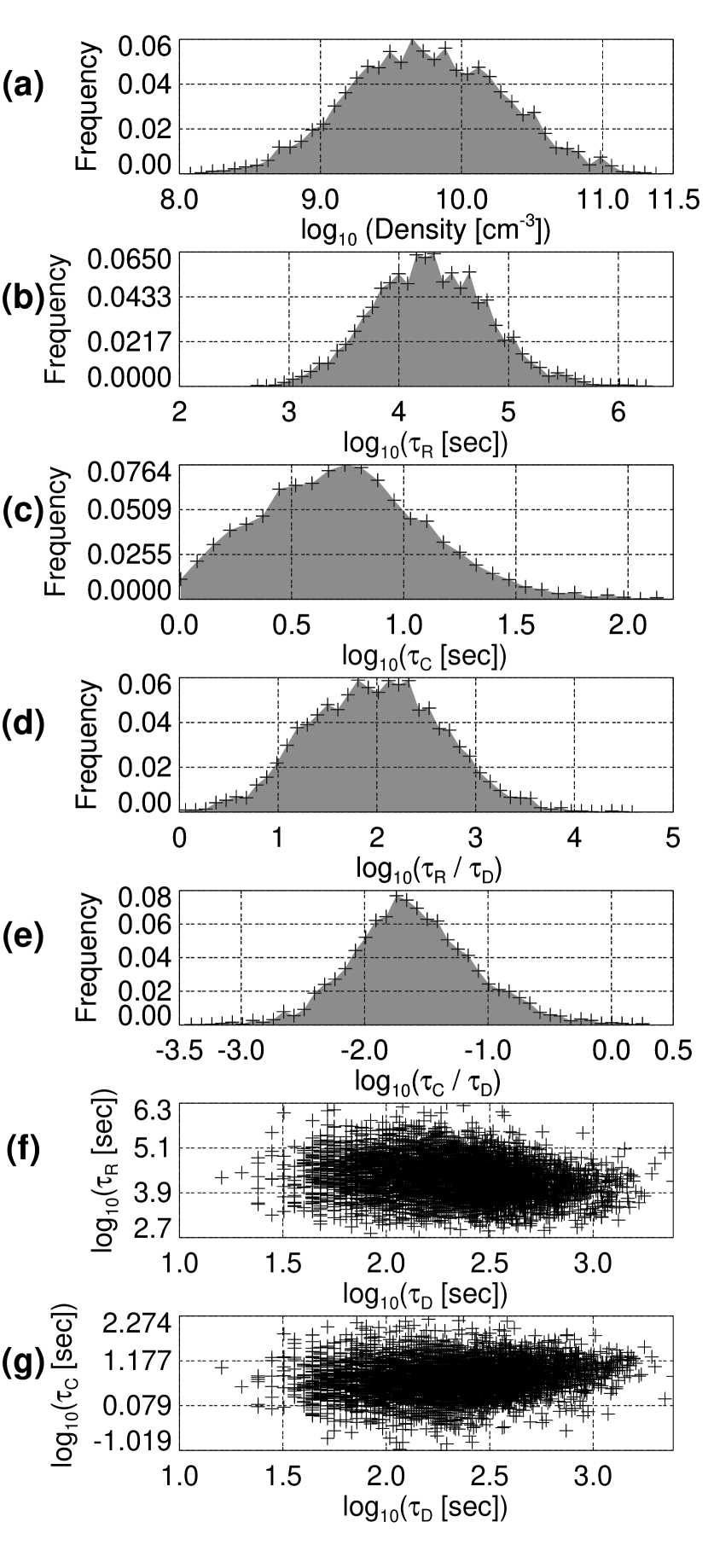
Figure 2: Flare parameters assuming a filling factor $\phi$ of unity. Plotted are distributions of the logarithms of (a) electron density $n_{e}$, (b) calculated values of the resistive cooling time $\tau_{R}$ and (c) the conductive cooling time $\tau_{C}$, (d) the ratio of radiative to flare decay times $\tau_{R}/\tau_{D}$, and (e) the ratio of conductive cooling times to flare decay times $\tau_{C}/\tau_{D}$. Panels (f) and (g) are scatter plots of the logarithms of $\tau_{R}$ vs. $\tau_{D}$ and $\tau_{C}$ vs. $\tau_{D}$, respectively.

The density estimates presented in Hannah et al. (2008) employed Eq. (2) which assumes a filling factor of unity. The distribution of the logarithm of $n_{e}$ under this assumption for the data in the present study is plotted in Fig. 2(a). The mean electron density of the distribution in Fig. 2(a) is $n_{e}\simeq 10^{9.8}\ {\rm cm}^{-3}$. As noted earlier, this mean density is a lower bound on the true mean density of the flares in the present study.

Using the density derived for each individual event, we estimate the radiative and conductive cooling times using Eqs. (5) and (6) for each microflare. The raw values for the distributions of the logarithms of the resultant radiative and conductive cooling times are plotted in Figs. 2(b) and (c), respectively. The median values of the calculated $\tau_{R}$ and $\tau_{C}$ are $2.06\times 10^{4}$ sec and 5.43 sec, respectively. Figs. 2(d) and (e) show the same values normalized to the flare’s observed decay times $\tau_{D}$. Panels (f) and (g) show a scatter plot of the logarithm of the calculated cooling times compared to the logarithm of their decay times, showing that the time scales are essentially uncorrelated. Panel (d) shows that the radiative cooling times are distributed around a peak about 100 times longer than $\tau_{D}$, while panel (e) shows that the conductive cooling times are distributed around a peak almost 100 times smaller than $\tau_{D}$, i.e., $\tau_{C}\ll\tau_{D}\ll\tau_{R}$. This strongly contradicts the hypothesis in Eq. (7). Note, this assessment assumes that it is reasonable to compare the measured decay time to instantaneous e-folding times from the scaling. Since they may differ, this could introduce systematic errors in the comparison. However, we suspect that it is not enough to account for the large separation in scales inferred here.

Assuming the plasma parameters we use (including the density) are correct, it is difficult to envision a physical explanation which could justify the disparity in time scales because one expects a flare to decay on a time-scale determined by the shortest available dissipation time. From this perspective, it is difficult to understand how, in the presence of strong conductive cooling, the actual decay time can be much longer than the conductive time-scale. A likely cause is the assumption that $\phi=1$, which we now relax.

In order to address the four orders of magnitude disparity which appears to exist between the conductive and radiative decay times, we assume Eq. (7) holds and use it to solve for the density and filling factor. We then check to see if this assumption helps us arrive at an internally consistent set of flare decay time scales. Equating Eqs. (5) and (6) and solving for $n_{e}$ gives

$$n_{e}=\sqrt{\frac{4\kappa(T)T}{L^{2}\Lambda(T)}}.$$ (8)

This is equivalent to the classical analysis of Rosner et al. (1978). Since $\kappa$ is a (weak) function of density due to the Coulomb logarithm, we employ an iterative technique to self-consistently solve for the density. The procedure is to assume $\phi=1$ to obtain a zeroth order estimate $n_{0}$ which is used to calculate the zeroth order $\kappa_{0}$. The next order of density $n_{1}$ is then determined from the previous $\kappa_{0}$. This is continued until convergence. We find $n_{e}$ is determined to eight significant figures after ten iterations and that the iterative procedure changes $\Lambda(T)$ by only 10%. Using this value of the density, the filling factor is obtained from Eq. (3) and cooling times are obtained from Eqs. (5) and (6).

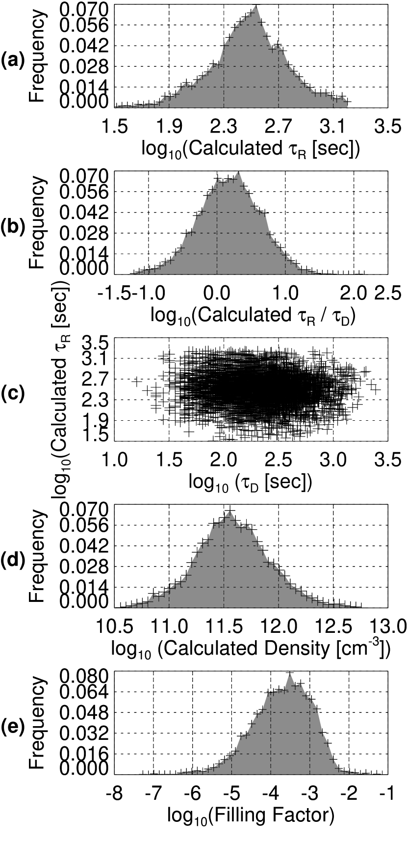
Figure 3: Flare parameters assuming radiative and conductive cooling times are equal. Plotted are distributions of the logarithms of (a) the radiative cooling time $\tau_{R}$ and (b) the ratio of radiative to flare decay times $\tau_{R}/\tau_{D}$. The conductive cooling time is equivalent to the radiative cooling time by construction. Panel (c) shows a scatter plot of the logarithms of $\tau_{R}$ vs. $\tau_{D}$. Also plotted are the logarithms of (d) the electron density $n_{e}$, and (e) the filling factor $\phi$.

The results of this analysis are displayed in Fig. 3. Panel (a) shows the distribution of the logarithm of the radiative cooling time $\tau_{R}$, while (b) shows the distribution for the logarithm of $\tau_{R}$ normalized to the flare decay time $\tau_{D}$. The conductive cooling times $\tau_{C}$ are equal to $\tau_{R}$ by construction. The median value of $\tau_{R}$ is 325 sec, which is within a factor of 1.7 of the median value of $\tau_{D}$. This is reiterated in panel (c), which is a scatter plot of $\tau_{R}$ and $\tau_{D}$. The values do not appear to be correlated, but they are clearly of the same order. It is surprising that the scales of the cooling times are essentially equal to a key empirical time scale, $\tau_{D}$; nothing in the model requires that such a similarity should emerge from the analysis. Of course, there are uncertainties associated with the comparison of observed decay times and predicted e-folding scaling times, but the present results lend observational support that a model with $\tau_{C}\sim\tau_{R}\sim\tau_{D}$ (as has been often assumed before) is consistent, at least for the present data set.

Panel (d) shows the logarithm of the resultant values for the calculated densities from Eq. (8). The distribution has a mean of $n_{e}\sim 10^{11.6}\ {\rm cm}^{-3}$, which is nearly two orders of magnitude higher than the reported values in Hannah et al. (2008) and plotted in Fig. 2(a). The inferred filling factors, the logarithm of which is shown in panel (e), have a mean of $\phi\sim 10^{-3.7}$. We discuss these results further in the following section.

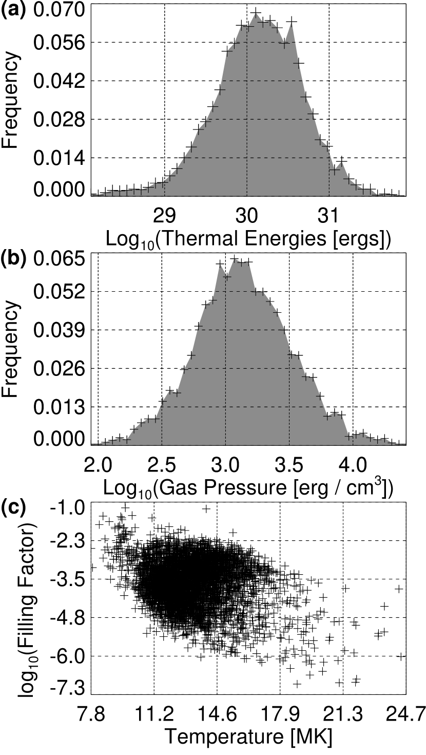
Figure 4: Distributions of the logarithms of (a) the calculated thermal energy $W_{T}=3n_{e}k_{B}T_{e}V$ and (b) gas pressure $P=2n_{e}k_{B}T_{e}$ using the values of density from Fig. 3(a). (c) Scatter plot of the logarithm of the filling factor $\phi$ against electron temperature $T_{e}$.

Using the calculated densities, one can calculate other properties of the flare loops. The logarithm of the total thermal energy $W_{T}=3n_{e}k_{B}T_{e}V$ in the flare loops is shown in Fig. 4(a), with a median value of $1.57\times 10^{30}$ erg. The distribution of the logarithm of the calculated gas pressures $P=2n_{e}k_{B}T_{e}$ is shown in Fig. 4(b), with a median value of $1.43\times 10^{3}$ erg cm^-1. Figure 4(c) is a scatter plot of the logarithm of the calculated filling factor $\phi$ against the electron temperature $T_{e}$. The filling factor is smaller for higher temperature loops, which is a consequence of Eqs. (3) and (8).

We now discuss the effect of uncertainties in the present analysis. As discussed in Sec. 2, the statistical errors in the length $L$, emission measure $EM$, and temperature $T$ are approximately $20\%,10\%$, and $1\%$ (Christe et al., 2008; Hannah et al., 2008). Standard error propagation techniques imply uncertainties for calculated cooling times of $40\%$, densities $20\%$, and filling factors $40\%$, which are sizable but not unreasonably large.

A few potential sources of systematic errors have been noted. They include assuming that the measured decay time $\tau_{D}$ corresponds to an e-folding decay time from a scaling analysis, that the representative loop length is assumed to be equal to the values obtained by Hannah et al. (2008) determined from particles at energies far above thermal energies, and that there is no external heating at the time of peak flare temperature.

5 DISCUSSION

In this paper, RHESSI microflare data are used to estimate the volumetric filling factor and the electron density of microflare loops using an analysis of cooling times. If the filling factor is assumed to be unity, then the conductive cooling time of the loop is much smaller than the observed decay time, which itself is much smaller than the radiative decay time. This is difficult to justify physically. Alternately, if one invokes the hypothesis that the radiative and conductive cooling times are comparable at the moment when the flare temperature passes through its maximum value (and that cooling due to expansion and flare heating are negligible at that time), one can solve for the filling factor and density. Mean values for the whole distribution are $\phi\sim 10^{-3.7}$ and $n_{e}\sim 10^{11.6}\ {\rm cm}^{-3}$. Our weakest assumption is that flare heating stops at the peak time of hard X-rays. Since the hard X-ray time profile is a convolution of heating and cooling, heating does not necessarily stop at the hard X-ray peak time. If heating is present during the decay, even at a low level, the cooling times could be longer than derived for the case without heating, and the filling factor could be larger than derived here.

Our estimate of mean densities are higher than those reported by Hannah et al. (2008). The authors are aware of only one other systematic study of microflare loop densities or filling factors (Moore et al., 1999), who used Yohkoh to study two microflare strands. Using an identical analytical technique as the present study, they found densities between $n_{e}\sim 10^{10}\ {\rm cm}^{-3}$ and $10^{11.6}\ {\rm cm}^{-3}$, with filling factors between $10^{-3.2}$ and $10^{-2.8}$. Thus, the values in the two microflares studied by (Moore et al., 1999) from Yohkoh are in good agreement with results from the large RHESSI data set studied here.

We now compare the present results with observations of large flares. Culhane et al. (1994) found $\phi\sim 1$ and $n_{e}\sim 3\times 10^{11}\ {\rm cm}^{-3}$ for an M-class flare, Varady et al. (2000) found $\phi\sim 0.01-0.2$ and $n_{e}\sim 7\times 10^{9}-1.5\times 10^{10}\ {\rm cm}^{-3}$ for a C-class flare, Aschwanden & Alexander (2001) found $\phi\sim 1$ and $n_{e}\sim 1.5\times 10^{10}\ {\rm cm}^{-3}$ for the Bastille Day flare, Teriaca et al. (2006) found $\phi\sim 0.2-0.5$ and $n_{e}\sim 10^{10}\ {\rm cm}^{-3}$ for a C-class flare, and Raymond et al. (2007) found $\phi\geq 0.01$ and $n_{e}\sim 10^{11}\ {\rm cm}^{-3}$ for X-class flares. Other examples of filling factors include 0.3 in active region loops (Landi et al., 2009), 0.04-0.07 in coronal holes (Abramenko et al., 2009), and near unity in many coronal hole jets (Doschek et al., 2010) but 0.03 in another study (Chifor et al., 2008). As noted earlier, the determination of filling factors can depend on detector resolution and wavelength. Nonetheless, the filling factors obtained here for microflares are at least 10 times smaller than those reported for large flares, which is likely statistically significant. Densities are slightly higher for microflares in the present study than for larger flares in previous studies.

Given the characteristics of the microflare data set considered here compared to large flares, it is perhaps not surprising that the filling factors are small. The microflare loops in the present study occur in active regions, just as large flares do. The mean sizes of the loops in the present study are comparable to those of larger flares. The loops have energies of $n_{e}k_{B}TV\sim 10^{28}{\rm\ ergs}$ deposited into them by the flare (using characteristic values from Fig. 1), which is about $10^{4}$ times smaller than large flares. Thus, the loops are of similar size but acquire less energy, which could lead to a smaller filling factor. To estimate the size of the region for which radiation is detected, we note the radiating volume is $V_{*}=\phi V$. Assuming that the length of the radiating plasma is $L$, the effective width $w_{*}$ of the radiating plasma is given by $V_{*}\sim\pi(w_{*}/2)^{2}L$. For the present parameters, this implies loops with total thickness $w_{*}\sim\phi^{1/2}w\simeq w/100\simeq 4\times 10^{6}\ {\rm cm}$, which would imply there is an unseen substructure of thin strands within the flare loops.

Various lines of evidence indicate that there are smaller-scale structures in the corona, e.g. Mullan (1990). Radio polarization data point to the existence of structures in the corona which are $\sim~{}100$ km in size (Melrose, 1975). The possibility that 100 km structures are associated with collapsing magnetic reconnection sites in the corona was discussed by Mullan (1980): using constraints on the collapse time-scales and coronal Alfvén speeds, transverse dimensions of order 100 km were found to be typical of reconnection sites in the corona. More recently, there is evidence that X-class flare loops are composed of thin threads from high resolution observations, with structure at scales of a few arcseconds ($1^{\prime\prime}\simeq 10^{8}{\rm\ cm}$) and below (Dennis & Pernak, 2009; Kontar et al., 2010; Krucker et al., 2010). There is also abundant evidence from the footpoints of flaring loops that most of the emission is spatially unresolved, such as in TRACE white-light flares (Hudson et al., 2006). Xu et al. (2006) found a core region within a halo region in two X-class white-light flares, reporting a ratio of the area of the core to the halo of 4% and 25%, respectively. Also, simulations of loops comprised of many small scale filaments were able to reproduce cooling characteristics of large flare loops observed with TRACE (Warren et al., 2003). Thus, the conclusion that there is small substructure of flare loops is not without precedent.

The prediction of small scale loops has implications for the heating mechanism of the flare loops. Hannah et al. (2008) estimated that the non-thermal power in accelerated electrons during the time of peak emission in the RHESSI microflares is $10^{26}\ {\rm erg\ s}^{-1}$. For loops of area $10^{14}{\rm\ cm}^{2}$ as predicted by the present results, the energy deposition rate per unit area would be $10^{12}{\rm\ erg\ s}^{-1}{\rm\ cm}^{-2}$. This is an enormous value, as discussed in Krucker et al. (2010). Hence, if the filling factor is indeed $\sim 10^{-4}$, then microflares are unlikely heated by electron beams. A recent model that the flare energy is transported by Alfvén waves (Fletcher & Hudson, 2008) would not be ruled out by the data.

An interesting result of the present study is that the conductive and radiative cooling times derived by assuming their equality at the time of maximum temperature are comparable to the observed microflare decay times. A possible ramification of this result is that it lends credence to the assumption that the conductive and radiative times are comparable to the decay time, $\tau_{R}\sim\tau_{C}\sim\tau_{D}$. This is relevant to stellar flare studies in which plasma parameters were obtained under such assumptions (Haisch, 1983; Stern et al., 1983). In addition, a previous study of stellar flares (Mullan et al., 2006) found results of this model are largely consistent with independently determined plasma parameters. If one believes that the scaling analysis cooling times actually represent physical cooling times for loops, the result suggests that conductive and radiative cooling act at comparable levels to cool flare loops, at least for the microflares in the present study.

Future work could include efforts to incorporate physical effects left out of the model as summarized at the end of Sec. 3. Also, future studies could further try to minimize the systematic errors discussed in Sec. 4. These can be addressed both with observations and with numerical modeling. Also, the study of the cooling times of individual events will help determine the validity of the cooling time analysis.

The authors thank G. Holman and B. Dennis for helpful conversations. RNB and PAC gratefully acknowledge support by NSF grant PHY-0902479, NASA’s EPSCoR Research Infrastructure Development Program and the West Virginia University Faculty Senate Research Grant program. DJM is supported in part by the Delaware Space Grant. IGH is supported by a STFC rolling grant and by the European Commission through the SOLAIRE Network (MTRN-CT-2006-035484). RPL is supported in part by the WCU grant (No. R31-10016) funded by the Korean Ministry of Education, Science and Technology. HSH, RPL, and SK are supported through NASA contract NAS 5-98033 for RHESSI.

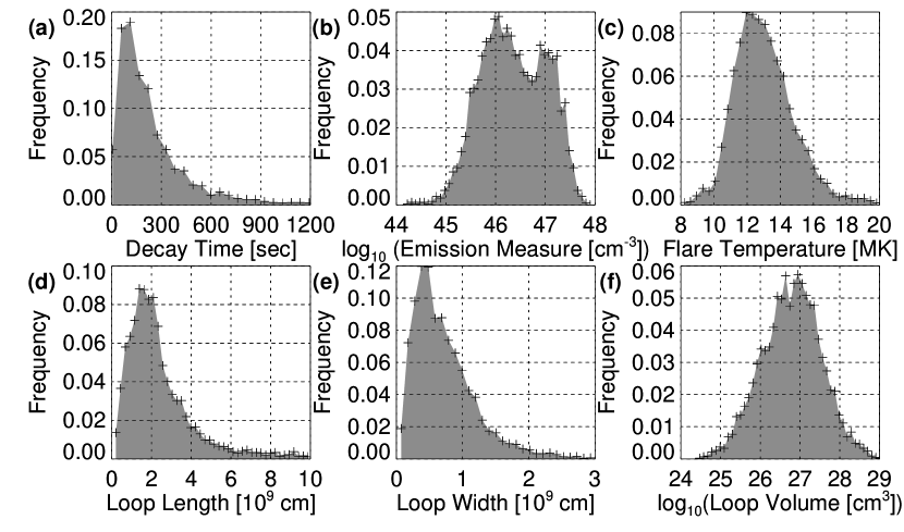
Figure 1: Distributions of raw data used in the present study using the methods described by Christe et al. (2008) and Hannah et al. (2008). Plotted are (a) flare decay time $\tau_{D}$, (b) the logarithm of the emission measure $EM$, (c) the logarithm of the temperature $T$, (d) flare loop full-length $L$, (e) flare loop full-width $w$, and (f) the logarithm of the flare loop volume $V$.

References

- Abramenko et al. (2009) Abramenko, V., Yurchyshyn, V., & Watanabe, H. 2009, Solar Phys., 260, 43
- Antiochos (1980) Antiochos, S. K. 1980, Ap. J., 241, 385
- Antiochos et al. (2000) Antiochos, S. K., DeLuca, E. E., Golub, L., & McMullen, R. A. 2000, Ap. J., 542, L151
- Antiochos & Sturrock (1976) Antiochos, S. K. & Sturrock, P. A. 1976, Solar Phys., 49, 359
- Antiochos & Sturrock (1978) —. 1978, Ap. J., 220, 1137
- Antiochos & Sturrock (1982) —. 1982, Ap. J., 254, 343
- Aschwanden (2007) Aschwanden, M. J. 2007, Adv. Space Res., 39, 1867
- Aschwanden & Alexander (2001) Aschwanden, M. J. & Alexander, D. 2001, Solar Phys., 204, 93
- Aschwanden & Aschwanden (2008) Aschwanden, M. J. & Aschwanden, P. D. 2008, Ap. J., 674, 544
- Aschwanden et al. (2008) Aschwanden, M. J., Stern, R. A., & Gudel, M. 2008, Ap. J., 672, 659
- Aschwanden et al. (2000) Aschwanden, M. J., Tarbell, T. D., Nightingale, R. W., Schrijver, C. J., Title, A., Kankelborg, C. C., Martens, P., & Warren, H. P. 2000, Ap. J., 535, 1047
- Aschwanden & Tsiklauri (2009) Aschwanden, M. J. & Tsiklauri, D. 2009, Ap. J. Supp. Ser., 185, 171
- Bradshaw & Cargill (2010) Bradshaw, S. J. & Cargill, P. J. 2010, Ap. J., 710, L39
- Cargill (1993) Cargill, P. J. 1993, Sol. Phys., 147, 263
- Cargill & Klimchuk (2004) Cargill, P. J. & Klimchuk, J. A. 2004, Ap. J., 605, 911
- Cargill et al. (1995) Cargill, P. J., Mariska, J. T., & Antiochos, S. K. 1995, Ap. J., 439, 1034
- Caspi & Lin (2010) Caspi, A. & Lin, R. P. 2010, Ap. J. Lett., submitted
- Cassak et al. (2008) Cassak, P. A., Mullan, D. J., & Shay, M. A. 2008, Ap. J. Lett., 676, L69
- Chifor et al. (2008) Chifor, C., Young, P. R., Isobe, H., Mason, H. E., Tripathi, D., Hara, H., & Yokoyama, T. 2008, Astron. Astrophys., 481, L57
- Christe et al. (2008) Christe, S., Hannah, I. G., Krucker, S., McTiernan, J., & Lin, R. P. 2008, Ap. J., 677, 1385
- Crosby et al. (1993) Crosby, N. B., Aschwanden, M. J., & Dennis, B. R. 1993, Solar Phys., 143, 275
- Culhane et al. (1994) Culhane, J. L., Phillips, A. T., Indakoide, M., Kosugi, T., Fludra, A., Kurokawa, H., Makishima, K., Pike, C. D., Sakao, T., Sakurai, T., Doschek, G. A., & Bentley, R. D. 1994, Solar Phys., 153, 307
- Culhane et al. (1970) Culhane, J. L., Vesecky, J. F., & Phillips, K. J. H. 1970, Solar Phys., 15, 394
- Dennis (1985) Dennis, B. R. 1985, Solar Phys., 100, 465
- Dennis & Pernak (2009) Dennis, B. R. & Pernak, R. L. 2009, Ap. J., 698, 2131
- Doschek et al. (1982) Doschek, G. A., Boris, J. P., Cheng, C.-C., Mariska, J. T., & Oran, E. S. 1982, Ap. J., 258, 373
- Doschek et al. (2010) Doschek, G. A., Landi, E., Warren, H. P., & Harra, L. K. 2010, Ap. J., 710, 1806
- Feldman et al. (1997) Feldman, U., Doschek, G. A., & Klimchuk, J. A. 1997, Ap. J., 474, 511
- Feldman et al. (1995) Feldman, U., Laming, J. M., & Doschek, G. A. 1995, Ap. J., 451, L79
- Fletcher et al. (in press) Fletcher, L., Dennis, B. R., Hudson, H. S., Krucker, S., Phillips, K., Veronig, A., Battaglia, M., Bone, L., Chen, Q., Gallagher, P., Grigis, P. T., Ji, H., Liu, W., Milligan, R. O., & Temmer, M. 2011, Space Sci. Rev., in press
- Fletcher & Hudson (2008) Fletcher, L. & Hudson, H. S. 2008, Ap. J., 675, 1645
- Forbes & Acton (1996) Forbes, T. G. & Acton, L. W. 1996, Ap. J., 459, 330
- Haisch (1983) Haisch, B. M. 1983, in IAU Colloq. 71, Activity in Red-Dwarf Stars, ed. P. B. Byrne & M. Rodono (Dordrecht: Reidel), 255
- Hannah et al. (2008) Hannah, I. G., Christe, S., Krucker, S., Hurford, G. J., Hudson, H. S., & Lin, R. P. 2008, Ap. J., 677, 704
- Hannah et al. (2010) Hannah, I. G., Hudson, H. S., Battaglia, M., Christe, S., Kasparova, J., Kundu, M., Krucker, S., & Veronig, A. 2011, Space Sci. Rev., in press
- Hudson et al. (2006) Hudson, H. S., Wolfson, C. J., & Metcalf, T. R. 2006, Solar Phys., 234, 79
- Jiang et al. (2006) Jiang, Y. W., Liu, S., Liu, W., & Petrosian, V. 2006, Ap. J., 638, 1140
- Klimchuk et al. (2008) Klimchuk, J. A., Patsourakos, S., & Cargill, P. J. 2008, The Astrophysical Journal, 682, 1351
- Kontar et al. (2010) Kontar, E. P., Hannah, I. G., Jeffrey, N. L. S., & Battaglia, M. 2010, Ap. J., 717, 250
- Krucker et al. (2010) Krucker, S., Hudson, H. S., Benz, A. O., Csillaghy, A., & Lin, R. P. 2010, Ap. J., submitted
- Landi et al. (2009) Landi, E., Miralles, M. P., Curdt, W., & Hara, H. 2009, Ap. J., 695, 221
- Lin et al. (1992) Lin, J., Zhang, Z., Wang, Z., & Smartt, R. N. 1992, Astron. Astrophys., 253, 557
- Lin et al. (2002) Lin, R. P., Dennis, B. R., Hurford, G. J., Smith, D. M., Zehnder, A., Harvey, P. R., Curtis, D. W., Pankow, D., Turin, P., Bester, M., Csillaghy, A., Lewis, M., Madden, N., van Beek, H. F., Appleby, M., Raudorf, T., McTiernan, J., Ramaty, R., Schmahl, E., Schwartz, R., Krucker, S., Abiad, R., Quinn, T., Berg, P., Hashii, M., Sterling, R., Jackson, R., Pratt, R., Campbell, R. D., Malone, D., Landis, D., Barrington-Leigh, C. P., Slassi-Sennou, S., Cork, C., Clark, D., Amato, D., Orwig, L., Boyle, R., Banks, I. S., Shirey, K., Tolbert, A. K., Zarro, D., Snow, F., Thomsen, K., Henneck, R., Mchedlishvili, A., Ming, P., Fivian, M., Jordan, J., Wanner, R., Crubb, J., Preble, J., Matranga, M., Benz, A., Hudson, H., Canfield, R. C., Holman, G. D., Crannell, C., Kosugi, T., Emslie, A. G., Vilmer, N., Brown, J. C., Johns-Krull, C., Aschwanden, M., Metcalf, T., & Conway, A. 2002, Solar Phys., 210, 3
- Lin et al. (1984) Lin, R. P., Schwartz, R. A., Kane, S. R., Pelling, R. M., & Hurley, K. C. 1984, Ap. J., 283, 421
- Melrose (1975) Melrose, D. B. 1975, Solar Phys., 43, 79
- Moore et al. (1980) Moore, R., McKenzie, D. L., Svestka, Z., Widing, K. G., Antiochos, S. K., Dere, K. P., Dodson-Prince, H. W., Hiei, E., Krall, K. R., Krieger, A. S., Mason, H. E., Petrasso, R. D., Pneuman, G. W., Silk, J. K., Vorpahl, J. A., & Withbroe, G. L. Solar Flares (Colorado Associated University Press)
- Moore et al. (1999) Moore, R. L., Falconer, D. A., Porter, J. G., & Suess, S. T. 1999, Ap. J., 526, 505
- Mullan (1980) Mullan, D. J. 1980, Ap. J., 237, 244
- Mullan (1990) —. 1990, Astron. Astrophys., 232, 520
- Mullan et al. (2006) Mullan, D. J., Mathioudakis, M., Bloomfield, D. S., & Christian, D. J. 2006, Ap. J. Supp. Ser., 164, 173
- Nita et al. (2002) Nita, G. M., Gary, D. E., Lanzerotti, L. J., & Thomson, D. J. 2002, Ap. J., 570, 423
- Paczuski et al. (2005) Paczuski, M., Boettcher, S., & Baiesi, M. 2005, Phys. Rev. Lett., 95, 181102
- Raymond et al. (2007) Raymond, J. C., Holman, G., Ciaravella, A., Panasyuk, A., Ko, Y.-K., & Kohl, J. 2007, Ap. J., 659, 750
- Reeves & Warren (2002) Reeves, K. K. & Warren, H. P. 2002, Ap. J., 578, 590
- Rosner et al. (1978) Rosner, R., Tucker, W. H., & Vaiana, G. S. 1978, Ap. J., 220, 643
- Serio et al. (1981) Serio, S., Peres, G., Vaiana, G. S., Golub, L., & Rosner, R. 1981, Ap. J., 243, 288
- Shibata & Yokoyama (1999) Shibata, K. & Yokoyama, T. 1999, Ap. J., 526, L49
- Spitzer & Härm (1953) Spitzer, L. & Härm, R. 1953, Phys. Rev., 89, 977
- Stern et al. (1983) Stern, R. A., Underwood, J. H., & Antiochos, S. K. 1983, Ap. J., 264, L55
- Sturrock (1980) Sturrock, P. A. 1980, Solar flares: A monograph from SKYLAB Solar Workshop II (Colorado Associated University Press)
- Svestka (1987) Svestka, Z. 1987, Solar Phys., 108, 411
- Svestka et al. (1987) Svestka, Z. F., Fontenla, J. M., Machado, M. E., Martin, S. F., & Neidig, D. F. 1987, Solar Phys., 108, 237
- Teriaca et al. (2006) Teriaca, L., Falchi, A., Falciani, R., Cauzzi, G., & Maltagliati, L. 2006, Astron. Astrophys., 455, 1123
- Tsiropoula et al. (2007) Tsiropoula, G., Tziotziou, K., Wiegelmann, T., Zachariadis, T., Gontikakis, C., & Dara, H. 2007, Solar Phys., 240, 37
- Varady et al. (2000) Varady, M., Fludra, A., & Heinzel, P. 2000, Astron. Astrophys., 355, 769
- Vrsnak et al. (2006) Vrsnak, B., Temmer, M., Veronig, A., & Karlicky, M. 2006, Solar Phys., 234, 273
- Warren et al. (2003) Warren, H. P., Winebarger, A. R., & Mariska, J. T. 2003, Ap. J., 593, 1174
- Wheatland (2000) Wheatland, M. S. 2000, Ap. J., 536, L109
- Xu et al. (2006) Xu, Y., Cao, W., Liu, C., Yang, G., Jing, J., Denker, C., Emslie, A. G., & Wang, H. 2006, Ap. J., 641, 1210