Timing and spectral study of XB 1254–690 using new RXTE PCA data

Abstract

We have analyzed the new Rossi X-ray Timing Explorer Proportional Counter Array data of the atoll neutron star (NS) low-mass X-ray binary (LMXB) system XB 1254–690. The colour-colour diagram shows that the source was in the high-intensity banana state. We have found two low-frequency candidate peaks with single trial significances of $\approx 2.65\times 10^{-8}$ and $\approx 7.39\times 10^{-8}$ in the power spectra. After taking into account the number of trials, the joint probability of appearance of these two peaks in the data set only by chance is $\sim 4.5\times 10^{-4}$, and hence a low-frequency QPO can be considered to be detected with a significance of $\sim 4.5\times 10^{-4}$, or, $\sim 3.5\sigma$ for the first time from this source. We have also done the first systematic X-ray spectral study of XB 1254–690, and found that, while one-component models are inadequate, three-component models are not required by the data. We have concluded that a combined broken-powerlaw and Comptonization model best describes the source continuum spectrum among 19 two-component models. The plasma temperature ($\sim 3$ keV) and the optical depth ($\sim 7$) of the Comptonization component are consistent with the previously reported values for other sources. However, the use of a broken-powerlaw component to describe NS LMXB spectra has recently been started, and we have used this component for XB 1254–690 for the first time. We have attempted to determine the relative energy budgets of the accretion disc and the boundary layer using the best-fit spectral model, and concluded that a reliable estimation of these budgets requires correlations among time variations of spectral properties in different wavelengths.

1 Introduction

The persistent neutron star low mass X–ray binary (LMXB) system XB 1254–690 exhibits energy dependent intensity dips with the binary orbital period ($\sim 3.88$ hr), thermonuclear X-ray bursts, and flares (Griffiths et al., 1978; Courvoisier et al., 1986; Mason et al., 1980; Smale et al., 2002). This is a so-called “atoll” source (Bhattacharyya, 2007). An atoll source typically traces a ‘C’-like curve in its colour-colour diagram or CCD (van der Klis, 2006). The high-intensity lower part of this curve is known as the banana state (van der Klis, 2006). XB 1254–690 has always been found in the banana state, and has never been observed in the spectrally hard low-intensity island state (Bhattacharyya, 2007). Note that the position of a source on the CCD is usually correlated with the timing features observed from the source (van der Klis, 2006). Therefore, CCDs are useful to determine the source state, and hence to understand the related physics.

Fast brightness oscillations, i.e., burst oscillations, have been observed from thermonuclear bursts from several neutron star LMXBs (Strohmayer and Bildsten (2006); Bhattacharyya (2010) and references therein). This timing feature provides one of the two ways to measure neutron star spin frequencies for LMXB systems (Chakrabarty et al., 2003; Bhattacharyya, 2010). Bhattacharyya (2007) reported a suggestive evidence of 95 Hz oscillations from a thermonuclear burst from XB 1254–690. This indicates that the neutron star in this source spins with a frequency of 95 Hz, although further confirmation is required to establish this.

Various types of quasi-periodic oscillations (QPOs) are observed from neutron star LMXBs (van der Klis, 2006). Their frequencies are roughly between millihertz (mHz) and kilohertz (kHz). Properties of one type of QPOs are sometimes correlated with those of another, and typically these properties are correlated with the spectral state inferred from CCD. Therefore, the QPOs can be very useful to understand the accretion process around a neutron star. In addition, kHz QPOs can be useful to probe the strong gravity regime, and to measure the neutron star parameters (van der Klis, 2006; Bhattacharyya, 2010). However, any detection of a QPO from XB 1254–690 was never reported before this paper.

The continuum spectrum of a neutron star LMXB is typically well described with various models, giving different physical interpretations (Lin et al., 2007). For example, two classical spectral models, Eastern and Western, have been proposed for the high-intensity states (Mitsuda et al., 1989; White et al., 1988). The Eastern model consists of a multicolour blackbody from the disc and a Comptonized component from the boundary layer (the contact layer between the neutron star and the disc inner edge), while the Western model has a Comptonized emission from the disc and a single temperature blackbody from the boundary layer. Although further detailed studies have been done with more sources (e.g., Church & Balucińska-Church (2001); Christian & Swank (1997); Maccarone & Coppi (2003); Maitra & Bailyn (2004); Gilfanov et al. (2003); Olive et al. (2003); Wijnands (2001); Barret (2001)), a general consensus on the appropriate X-ray spectral model has not been achieved. It is therefore essential to do systematic spectral studies of neutron star LMXBs using all the reasonable physical models. Even before going into the details, the first aim of such a study will be to identify which spectral component originates from the boundary layer, and which one comes from the disc, and hence to find out the relative energy budgets of these two X-ray emitting components. These relative budgets not only will be useful to understand the accretion process and components, but also will be helpful to constrain the neutron star parameters and equation of state (EoS) models (Bhattacharyya et al., 2000; Bhattacharyya, 2002, 2010). Recently, Lin et al. (2007) have done such a systematic study for two neutron star LMXBs (Aql X–1 and 4U 1608–52). However, such a study has never been done for XB 1254–690.

In this paper, we report the first evidence of a QPO from XB 1254–690. Moreover, we give the results and interpretations of the first systematic X-ray spectral study of this source. In § 2, we mention the spectral and timing analysis methods, and report the results. In § 3, we discuss the interpretation and importance of the observational results.

2 Data Analysis and Results

The neutron star LMXB system XB 1254–690 was observed with Rossi X-ray Timing Explorer (RXTE) between Jan 16, 2008 (start time: 13:27:50; proposal no. P93062) and Mar 13, 2008 (end time: 19:42:08) for a total observation time of 283.42 ks (total 60 observations; good-time after excluding bursts, dips, flares, datagaps, etc. is 257.39 ks). We have used the corresponding Proportional Counter Array (PCA) data set for our analysis. We have searched for quasi-periodic oscillations (QPOs) in this data set, computed a CCD and a hardness-intensity diagram (HID), and fitted the continuum spectra with various models extensively. We have used Good Xenon data files for the timing analysis, and Standard2 (Std2) data files to perform spectral analysis and to compute the CCD and the HID.

2.1 Colour-Colour and Hardness-Intensity Diagram

We have shown a CCD and an HID of XB 1254–690 in Fig. 1. A CCD is a plot of a hard-colour vs a soft-colour. We have defined the soft-colour as the ratio of the background subtracted counts in the energy range 5.7–7.5 keV to that in 4.4–5.7 keV. Similarly, the hard-colour has been defined as the ratio of the background subtracted counts in 11.4–20.7 keV to that in 7.5–11.4 keV. An HID is a plot of hard-colour vs intensity. The intensity has been defined as the total background subtracted counts in the energy range 4.4–20.7 keV. These photon-counts have been calculated from the Std2 data of the RXTE PCA instrument. We have used only the PCU2 data, because this Proportional Counter Unit (PCU) operated during all the observations. Furthermore, we have used only the upper layers of PCU2 in order to get a better signal-to-noise ratio.

Fig. 1 shows that the source was in the banana state during all the observations. This is consistent with the earlier results (§ 1; see Bhattacharyya (2007)). We have detected two thermonuclear X-ray bursts, and several flares and dips in the lower banana state. The bursts have not exhibited signatures of photospheric radius expansion. In addition, we have not detected burst oscillations from these bursts.

2.2 Timing Analysis

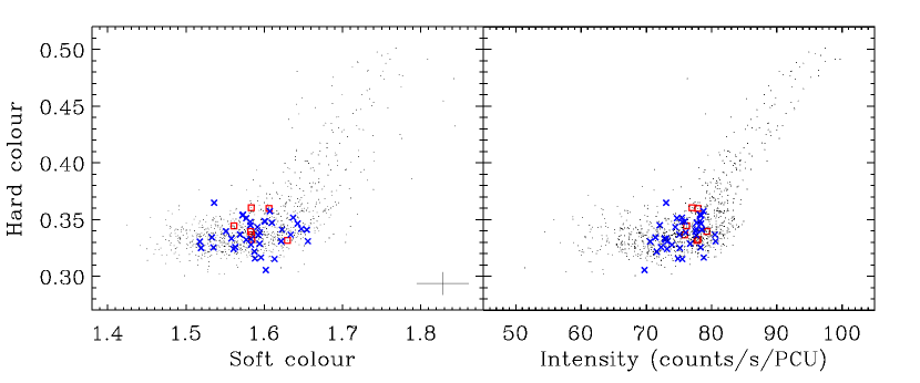
Figure 3: Colour-colour diagram (CCD; left panel) and hardness-intensity diagram (HID; right panel) of the neutron star LMXB XB 1254–690 (same as Fig. 1). The data corresponding to the 64.01 Hz candidate QPO and 48.63 Hz candidate QPO are marked with blue cross signs and red square signs respectively. This figure shows that both the candidate QPOs have appeared in the lower-banana (LB) state (§ 2.2).

We have not found any significant kHz QPO in the entire RXTE PCA data set. In order to search for low-frequency QPOs, we have calculated power spectra (for the entire PCA energy range) with a Nyquist frequency of 128 Hz for 250 s intervals, using the Good Xenon data from PCU2. We have found two candidate peaks around the frequency $\sim 50$ Hz. The stronger one has appeared at 64.01 Hz in the power spectrum corresponding to the observation done on Jan 21, 2008 (time: 10:44:08 to 14:49:08). We have got a peak power of 2.983, after averaging over forty 250 s intervals and merging four consecutive frequency bins (see Fig. 2, left panel). The latter has made the frequency resolution 0.016 Hz. The probability of obtaining a power this high in a single trial from the expected $\chi^{2}$ noise distribution (320 dof) is $\approx 2.65\times 10^{-8}$. In order to find this peak, we have searched 60 power spectra, each with 8000 frequencies. Therefore, multiplying with a number of trials of 480000, we have found a significance of $1.27\times 10^{-2}$, or $\approx 2.5\sigma$. The rms amplitude of this candidate QPO is $\approx 0.83$%. The other candidate peak of same frequency-width and of $\approx 7.39\times 10^{-8}$ single trial significance has been found at 48.63 Hz from the observations on Jan 17-18, 2008 (time: between 22:47:28 to 00:02:10). Its rms amplitude is $\approx 1.3$% (Fig. 2, right panel), and significance is $3.55\times 10^{-2}$ after multiplying with the number of trials of 480000. In Fig. 3, we have marked the data corresponding to the two candidate QPOs in the CCD and the HID. This figure shows that both the candidate QPOs have appeared in the lower-banana (LB) state.

With these two candidate peaks, next we ask the question what would be the probability of having two such peaks simultaneously in our data set containing 60 power spectra only by chance. The 480000 powers mentioned in the previous paragraph are expected to be independent of each other, otherwise the significance of each peak would increase by the decrease of the number of trials. Therefore, naively the probability that the two candidate peaks would appear simultaneously in our data set only by chance is $1.27\times 10^{-2}\times 3.55\times 10^{-2}=4.5\times 10^{-4}$. However, this number is expected to be an upper limit, i.e., this significance is expected to be better for the following reason. Suppose, there are $10^{5}$ data sets like ours. Then, on average, the first peak should appear in 1270 data sets, and the second peak should appear in 3550 data sets. Now we ask the question: in how many data sets at least one power would exceed the first candidate peak power (i.e., the larger power) and at least two powers would exceed the second candidate peak power (i.e., the smaller power). This number will be less than 45, which is the above mentioned naively expected value, because there would be a chance that in some of the data sets more than one power would exceed the first candidate peak power and/or more than two powers would exceed the second candidate peak power. If this is true then the $4.5\times 10^{-4}$ would be the conservative value of the significance of simultaneous appearence of the two candidate peaks in our data set. We have verified this logical conclusion using simulated data with a pure Poisson process in the next paragraph.

Our simulated time series and power spectra have been rigorously tested, and have passed the following tests among others: (1) the counts in 1/4096 s bins of the time series follow the Poisson statistics extremely well; (2) when the simulated Leahy power spectra are fitted with a constant, the best-fit value is consistent with 2 (an example value is $1.9995\pm 0.0014$ for a 1 ks time series with the observed count rate); (3) the cumulative power distribution of the simulated power spectra matches well with $\chi^{2}$ distribution with the appropriate degrees of freedom. We have generated 10 Ms of simulated data with the observed count rate, which has been divided into 10 groups, each with 1000 time series of 1 ks. Note that, while counting within one group gives a random value, the sample of 10 groups gives the mean and the standard deviation. We have assumed two values of power: $p_{1}$ and $p_{2}$ ($p_{1}>p_{2}$), and estimated the number ($N$) of 1 ks time series (within one group) with at least one power above $p_{1}$ and at least two powers above $p_{2}$ in the three following ways. (1) In the first way we have used the conservative significance mentioned in the previous paragraph. We have calculated the significance ($S1_{p1}$ and $S1_{p2}$ respectively) of $p_{1}$ and $p_{2}$ in a 1 ks time series. Then with $S1_{\rm joint}=S1_{p1}\times S1_{p2}$, the number $N$ would be $N_{\rm conservative}=1000S1_{\rm joint}$. (2) In the second way, we have taken into account the fact (mentioned in the previous paragraph) that $p_{1}$ may be exceeded more than once, and/or $p_{2}$ may be exceeded more than twice in a 1 ks time series. Therefore we have counted the number of 1 ks time series in which $p_{1}$ is exceeded, and divided this number with 1000 to estimate the significance $S2_{p1}$ of $p_{1}$. Similarly we have estimated the significance $S2_{p2}$ of $p_{2}$. Then with $S2_{\rm joint}=S2_{p1}\times S2_{p2}$, the number $N$ would be $N_{\rm realistic}=1000S2_{\rm joint}$. (3) In the third way, we have simply counted the number $N=N_{\rm counted}$. For various combinations of $p_{1}$ and $p_{2}$ values, we have found that $N_{\rm counted}$ is always consistent with $N_{\rm realistic}$, but always significantly less than $N_{\rm conservative}$. This verifies the logical conclusion of the previous paragraph, that $4.5\times 10^{-4}$ is the conservative value of the significance of simultaneous appearence of the two candidate peaks in our data set.

Note that the single trial significances (typically, say, $1.25\times 10^{-5}$ and $5.0\times 10^{-5}$) of our assumed $p_{1}$ and $p_{2}$ values are much worse than those of the candidate peaks. We have assumed such powers, because, (1) much larger powers would not change our conclusions; and (2) a similar simulation with the significances of the candidate peaks would need $\sim 3\times 10^{6}$ Ms simulated data, which would require $\sim 10^{8}$ GB of computer disc space and an unrealistic amount of time. Therefore, since the probability of the appearence of both the candidate peaks in our data set only by chance is less than $4.5\times 10^{-4}$, one of them can be a signal with the significance of $\sim 4.5\times 10^{-4}$. Since both of them are of low-frequency, a low-frequency QPO can be considered to be detected from XB 1254-690 with a significance of $\sim 4.5\times 10^{-4}$, or, $\sim 3.5\sigma$.

2.3 Spectral Analysis

The neutron star LMXB XB 1254–690 was observed with several X-ray observatories, e.g., BeppoSAX, Chandra (HETGS), XMM-Newton, RXTE (PCA) (Iaria et al., 2001, 2007; Díaz Trigo et al., 2006; Smale et al., 2002). In order to fit the continuum spectra, these papers reported the usage of a few XSPEC models, such as diskbb + comptt (or compst), powerlaw + bbody, cutoffpl + bbody. But a systematic analysis of the XB 1254–690 continuum spectra using all the reasonable XSPEC models was previously not done. As mentioned in §1, Lin et al. (2007) have recently performed a systematic analysis using various continuum spectral models for two neutron star LMXBs. In this spirit, we have done the first systematic continuum spectral analysis for XB 1254–690.

Let us first discuss the currently understood X-ray components of neutron star LMXBs. Such a source plausibly has two primary X-ray emitting regions: a geometrically thin accretion disc, and a boundary layer. Each of the disc and the boundary layer is expected to be optically thick, and hence to emit like a blackbody. However, note that the disc blackbody should be a multicolour blackbody, as the blackbody temperature should be a function of the radial distance from the centre of the neutron star (Bhattacharyya et al., 2000). In addition, the disc and/or the boundary layer may be covered by one or more coronae (hot electron-gas), which may reprocess (Comptonize) the emitted radiation. Therefore, depending on the nature of the cover (e.g., partial versus full, optical depth), the observed spectrum of each of the disc and the boundary layer may be a blackbody, or Comptonized, or a combination of both. In this paper, we have studied these various possibilities systematically, in order to identify the nature of the X-ray emitting components.

We have used the Std2 data of the upper layers of PCU2 in order to do the continuum spectral analysis. We have made two spectral files (one for the LB state, another for the UB state) corresponding to the largest uninterrupted observational “good time” data sets after filtering out the bursts, dips and flares. Since the LB data set (20.7 ks) is much larger than the UB data set (1.1 ks; see Fig. 4), we have first modelled the LB spectrum, which has helped us to decide on the procedure. Then we have modelled the UB spectrum following this procedure. We have done the fitting in the energy range of 2.5–18.0 keV using XSPEC, including 1% systematic instrumental error.

We have used the XSPEC models bbody, diskbb and comptt for a blackbody, a multicolour blackbody and a Comptonized radiation respectively. In addition, we have used powerlaw, cutoffpl and bknpower for the phenomenological models powerlaw, cut-off-powerlaw and broken-powerlaw respectively. We have used the last model following the work of Lin et al. (2007). Note that, while the first two models can represent the Comptonized radiation (Rybicki & Lightman, 1979), the broken-powerlaw model can be an approximation for Comptonization under complex conditions or in combination with another radiation process, such as synchrotron radiation (Lin et al., 2007).

First, we have checked whether a single component can fit the LB spectrum well. We have found that cutoffpl, multiplied with XSPEC Galactic neutral hydrogen absorption model wabs, gives the best fit among all the single components, and the corresponding $\chi^{2}_{\nu}$ (dof) is $\approx$ 3.23 (33). This clearly suggests that at least two model components are required to fit the continuum spectrum. In the two-component scenario, there can be the following possibilities: (1) both the accretion disc and the boundary layer are purely thermal (diskbb, bbody); (2) the disc emission is thermal, but the boundary layer emission is Comptonized; (3) the boundary layer emission is thermal, but the disc emission is Comptonized; and (4) both of them are Comptonized. Therefore, for the six XSPEC model components, which we have considered, there can be 19 two-component models (see Table 1). We have fitted the LB continuum spectrum with each of these 19 models, multiplied with wabs model. Note that we have frozen the neutral hydrogen column density $N_{\rm H}$ of wabs to $0.29\times 10^{22}$ cm^-2 (estimated with NASA’s HEASARC nH tool; see also Smale et al. (2002)) for every model fitting reported in this paper. This is because the RXTE PCA cannot reliably measure $N_{\rm H}$, which affects the X-ray spectrum mostly at lower energies. Among these 19 models only six models have given good fits ($\chi^{2}_{\nu}\leq 1$), while for all other models $\chi^{2}_{\nu}\geq 1.5$ (see Table 1). Therefore, we will consider only these six models (bknpower + diskbb, comptt + comptt, comptt + powerlaw, comptt + cutoffpl, bknpower + comptt, bknpower + cutoffpl) for further discussion. Note that, since several two-component models fit the LB spectrum well, we have not considered more complex models involving partially thermal and partially Comptonized emission from each of the disc and the boundary layer. Moreover, addition of an iron line to the spectral model does not improve the fitting significantly, and does not change the best-fit parameter values substantially.

Table 2 and Fig. 5 suggest that the six best models can be divided into two groups: the first group consists of bknpower + diskbb, bknpower + cutoffpl and bknpower + comptt, while the second group consists of comptt + cutoffpl, comptt + comptt and comptt + powerlaw. This is because, Table 2 shows that the flux-ratios of the components are close to 2 for all the models of group-I, with bknpower as the dominant model, while those are greater than 5.5 for all the models of group-II, with comptt as the dominant model. Moreover, Fig. 5 clearly shows that the normalizations and the shapes of the two component-curves of a model are very similar within a group, but differ significantly between the groups. Is it now possible to determine which group is preferred? We have found that the best-fit optical depth ($\approx 10^{-2}$) of a comptt component of the comptt + comptt model is unphysically small (discussed with Lev Titarchuk), and we propose to rule out this model on this ground. Moreover, the cutoffpl and powerlaw components of the comptt + cutoffpl and comptt + powerlaw models are likely to represent the “unphysical” comptt component (see Fig. 5). Therefore, we argue that each of the three models of group-II probably represent the same physical scenario, and hence the entire group is not preferred. As a result, we tentatively support the group-I models, and give the best-fit model parameter values in Table 3.

Can we now differentiate the three models of group-I? The normalization parameter of diskbb component is given by $(R_{\rm in}/D)^{2}\cos\theta$, where $R_{\rm in}$ is the apparent inner edge radius of the disc in km, $D$ is the distance in 10 kpc and $\theta$ is the observer’s inclination angle. We have assumed $D=10$ kpc (Díaz Trigo et al., 2006), and $\theta=60^{\rm o}-75^{\rm o}$ from the observed dips, and lack of eclipses (Motch et al., 1987; Courvoisier et al., 1986; Frank et al., 1987). The best-fit normalization of the diskbb component of bknpower + diskbb model is 0.27 (Table 3). Therefore, even with a conservative value of the colour factor ($f=2.0$), the maximum value of actual disc inner edge radius comes out to be $\approx 4$ km. This is less than any realistic value of a neutron star radius, and hence is unphysical. We therefore propose to rule out the bknpower + diskbb model. However, this does not necessarily rule out the bknpower + cutoffpl and bknpower + comptt models, because while diskbb is a thermal component, comptt, as well as cutoffpl (which probably is a phenomenological representation of comptt; see Fig. 5) are Comptonized components. Therefore, we suggest that bknpower + comptt is the preferred model of LB continuum spectrum of XB 1254–690 in the energy range of 2.5–18.0 keV.

We have then repeated the above-mentioned procedure for the UB continuum spectrum. Even for this spectrum, the single component models do not give a good fit, and among the 19 two-component models, the group-I models give the best reduced $\chi^{2}$: $\chi^{2}_{\nu}=1.31$ for bknpower + diskbb, $\chi^{2}_{\nu}=1.36$ for bknpower + cutoffpl and $\chi^{2}_{\nu}=1.39$ for bknpower + comptt. In comparison, the physical model comptt + comptt of group-II gives $\chi^{2}_{\nu}=1.83$. However, in case of UB spectrum, the $\chi^{2}_{\nu}$ values for several other two-component models are not very different from those for group-I models. Therefore, it is difficult to identify the correct UB spectral model from the current data set. Nevertheless, following the results of LB spectrum, and keeping in mind that the group-I models do give the best $\chi^{2}_{\nu}$ values, we suggest that the group-I models are the preferred models even for UB spectrum. Note that, unlike the LB spectrum, the bknpower component of the group-I models of UB spectrum is not the dominant component (see Fig. 6). The diskbb component of bknpower + diskbb model suggests an unphysically small disc inner edge radius ($<5.4$ km) even for the UB spectrum. Therefore, we propose that bknpower + comptt is the most suitable model to describe the UB continuum spectrum of XB 1254–690 in the energy range of 2.5–18.0 keV. The corresponding best-fit model parameter values are given in Table 4. Note that addition of an absorption line or edge to the UB spectral model does not affect our conclusions substantially.

3 Discussion

In this paper, we have studied the timing and spectral properties of the neutron star LMXB XB 1254–690. This atoll source was in the banana state during all the RXTE observations. We have not detected burst oscillations from the two bursts in the analyzed data set. This is not surprising, as only a fraction of bursts from burst oscillation sources show oscillations (Galloway et al., 2008). However, this somewhat reduces the significance of the plausible burst oscillation feature reported in Bhattacharyya (2007) by increasing the number of trials. We report the first evidence of QPOs from this source, with frequencies consistent with the $\sim 30-80$ Hz QPOs typically observed from atoll sources in intermediate to high states (van der Klis, 2006).

We have also done the first systematic study of X-ray continuum spectrum from XB 1254–690. We have fitted an LB spectrum and a UB spectrum with 19 models (see § 2.3 and Table 1). In both cases, a broken-powerlaw plus a Comptonization model (bknpower + comptt) is favoured, and the plasma temperature and the optical depth of the Comptonization component are consistent with the previously reported values for other sources (Lin et al., 2007). A broken-powerlaw component was never used to fit the XB 1254–690 continuum spectrum, although it has been recently successfully used for the spectral fitting of Aql X–1 and 4U 1608–52. This component can represent Comptonization, either under complex conditions or in combination with another radiation process (e.g., synchrotron; see § 2.3). These imply that the blackbody radiations from the disc and the boundary layer are entirely processed before reaching the observer. Note that the classical models Eastern and Western give a much worse fit than the bknpower + comptt model. For example, $\chi_{\nu}^{2}$ (dof) values for Eastern, Western and bknpower + comptt models are 1.96 (30), 1.50 (30) and 0.54 (28) respectively for the LB spectrum. Besides, the cutoffpl + bbody and diskbb + powerlaw models, which were previously used for XB 1254–690 (Smale et al., 2002; Iaria et al., 2007), give much worse fits ($\chi_{\nu}^{2}$ (dof): 1.65 (31) and 1.95 (32) respectively for LB). However, although a broken-powerlaw component gives the best fit, note that it is only a phenomenological model, and should be replaced with a physical model in the future in order to clearly understand the meaning of the best-fit parameter values. A physical model will also be necessary to interpret the high $\Gamma_{2}$ of the UB broken-powerlaw (Table 4), which indicates a quick cut-off after the first powerlaw component.

With the best-fit model in hand, we have attempted to determine the relative energy budgets of the disc and the boundary layer. For the LB spectrum, the flux from the bknpower component is about 2.1 times larger than the comptt component (Table 2). Therefore, assuming one component entirely originates from the disc and the other component fully comes out of the boundary layer, we can make the following conclusions using the Fig. 5 of Bhattacharyya et al. (2000). (1) The spin frequency depends on the chosen EoS model of the neutron star, with larger frequencies for softer EoS models. Therefore, an independent measurement of the stellar spin frequency can be useful to constrain the EoS models. (2) If the bknpower component originates from the disc, then the neutron star is spinning with a frequency close to the break-up frequency (irrespective of the EoS model). However, these simple conclusions may not be reliable for one or more of the following reasons. (1) Each of the spectral components may originate partially from the disc, and partially from the boundary layer. (2) Disc emission and/or boundary layer emission may be partially obscured. (3) Boundary layer emission (and also the inner disc emission) may be partially reprocessed by the disc. Besides, the bknpower flux is smaller than the comptt flux for the lower quality UB spectrum, although the spectral shapes and parameters of these two components are very similar to those of the LB spectrum (see Tables 3 and 4; Figs. 5 and 6). This difference in the normalization ratio of the two components may be due to one or more of the above three reasons. One main problem in identifying and understanding the emissions from various source components is the lack of simultaneous broadband (optical, UV and X-ray) data. The optical and UV emissions are expected to originate by the reprocessing of the X-ray photons at the outer disc, and hence the correlations among time variations of spectral properties (e.g., Balucinska et al. (2004)), especially in different wavelengths will significantly contribute to the understanding of the neutron star LMXB components. The proposed Astrosat satellite will be useful for such a study in the near future.

Table 1: A list of two-component models used to fit the RXTE PCA continuum spectra of the neutron star LMXB XB 1254–690 (§ 2.3).

Sr. No.	Fitting models	$\chi^{2}_{\nu}$ (dof)	Number of
			free parameters
1	diskbb + comptt	1.95 (30)	6
2	diskbb + powerlaw	1.95 (32)	4
3	diskbb + cutoffpl	1.97 (31)	5
4	diskbb + bknpower	0.52 (30)	6
5	comptt + bbody	1.50 (30)	6
6	powerlaw + bbody	2.24 (32)	4
7	cutoffpl + bbody	1.65 (31)	5
8	bknpower + bbody	2.39 (30)	6
9	diskbb + bbody	2.75 (32)	4
10	comptt + comptt	0.91 (28)	8
11	powerlaw + comptt	0.95 (30)	6
12	cutoffpl + comptt	0.91 (29)	7
13	bknpower + comptt	0.54 (28)	8
14	powerlaw + powerlaw	32.31 (32)	4
15	cutoffpl + powerlaw	2.33 (31)	5
16	bknpower + powerlaw	3.47 (30)	6
17	cutoffpl + cutoffpl	1.54 (30)	6
18	bknpower + cutoffpl	0.53 (29)	7
19	bknpower + bknpower	3.73 (28)	8

⁰All models have been multiplied with the wabs absorption model of XSPEC, with the fixed $N_{\rm H}=0.29\times 10^{22}$cm^-2.

¹Reduced $\chi^{2}$ (degrees of freedom) for the LB spectrum

²Multicolour blackbody model of XSPEC.

³A powerlaw model with high energy exponential cut off.

⁴A broken power law with break energy $E_{\rm break}$.

⁵A Comptonization model in XSPEC.

⁶Blackbody model in XSPEC.

Table 2: Flux values of XB 1254–690 from fitting of the LB continuum spectrum with the six two-component models, which give $\chi^{2}_{\nu}\leq 1$.

. Model Group-I Model Group-II Models bknpower bknpower bknpower comptt comptt comptt +diskbb +cutoffpl +comptt +cutoffpl +comptt +powerlaw $\chi^{2}_{\nu}$ (dof) 0.52(30) 0.53(29) 0.54(28) 0.91(29) 0.91(28) 0.95(30) Absorbed total flux 7.88 7.88 7.90 7.96 8.00 7.96 Unabsorbed total flux 8.02 8.02 8.04 8.11 8.15 8.11 Flux of the first component 5.28 5.60 5.44 7.25 7.27 6.88 Flux of the second component 2.74 2.42 2.60 0.86 0.87 1.23 Ratio of the two fluxes 1.92 2.31 2.09 8.42 8.45 5.59

¹In the range 2.5–18.0 keV and in unit of $10^{-10}$ ergs cm^-2 s^-1.

Table 3: Spectral fitting parameters of the LB state of XB 1254–690 for the three two-component models (see Table 2 and § 2.3). Best-fit values are accompanied with 90% errors.

Sr. No.	Model	Component	Parmeters	Best-fit values	Component	Parmeters	Best-fit values
1	bknpower+diskbb	bknpower	$\Gamma_{1}$	$2.40_{-0.091}^{+0.17}$	diskbb	Tin	$2.82_{-0.34}^{+0.20}$
			$E_{\rm break}$	$6.29_{-0.18}^{+0.18}$		norm	$0.27_{-0.062}^{+0.16}$
			$\Gamma_{2}$	$3.85_{-0.39}^{+0.83}$
			norm	$0.43_{-0.042}^{+0.057}$
2	bknpower+cutoffpl	bknpower	$\Gamma_{1}$	$2.43_{-0.10}^{+0.33}$	cutoffpl	$\alpha$	$-0.36_{-0.36}^{+1.1}$
			$E_{\rm break}$	$6.25_{-0.22}^{+0.31}$		$\beta$	$3.00_{-1.2}^{+1.4}$
			$\Gamma_{2}$	$3.83_{-0.36}^{+1.6}$		norm	$0.011_{-0.011}^{+0.025}$
			norm	$0.48_{-0.14}^{+0.066}$
3	bknpower+comptt	bknpower	$\Gamma_{1}$	$2.52_{-2.2}^{+0.80}$	comptt	T0	$1.12_{-1.1}^{+1.1}$
			$E_{\rm break}$	$6.26_{-0.26}^{+0.56}$		kT	$3.00_{-2.6}^{+7.7}$
			$\Gamma_{2}$	$3.89_{-0.45}^{+5.3}$		taup	$6.82_{-6.8}^{+183}$
			norm	$0.48_{-0.38}^{+1.2}$		norm	$0.02_{-0.013}^{+0.023}$

¹A broken power law:

$$A(E)=KE^{-\Gamma_{1}}\;\;\mathtt{for}\;\;E\leq E_{\rm break};$$

$$=KE_{\rm break}^{\Gamma_{2}-\Gamma_{1}}\times(E/1keV)^{-\Gamma_{2}}\;\;\mathtt{for}\;\;E\geq E_{\rm break}.$$

$E_{\rm break}$ is in keV.

²Temperature at inner disc radius (in keV).

³A power law with high energy exponential cut off:

$$A(E)=KE^{-\alpha}exp{(-E/\beta)}.$$

$\beta$ is in keV.

⁴Input soft photon (Wien) temperature (in keV).

⁵Plasma temperature (in keV).

⁶Optical depth of the corona.

Table 4: Spectral fitting parameters of the UB state of XB 1254–690 for a two-component model (see § 2.3). Best-fit values are accompanied with 90% errors.

Model	Component	Parmeters	Best-fit values	Component	Parmeters	Best-fit values
bknpower+comptt	bknpower	$\Gamma_{1}$	$2.32_{-0.32}^{+0.35}$	comptt	T0	$0.67_{-0.06}^{+0.07}$
		$E_{\rm break}$	$7.22_{-0.97}^{+0.40}$		kT	$2.79_{-0.12}^{+0.18}$
		$\Gamma_{2}$	$9.99_{-0.1}^{+0.008}$		taup	$7.78_{-1.7}^{+2.2}$
		norm	$0.12_{-0.07}^{+0.22}$		norm	$1.08_{-0.4}^{+0.1}$

¹Definitions and units of parameters are same as in Table 3.

²The large value of the photon index indicates a quick cut-off after the first powerlaw component (see § 3).

Figure 1: Colour-colour diagram (CCD; left panel) and hardness-intensity diagram (HID; right panel) of the neutron star LMXB XB 1254–690. Here the soft-colour is defined as the ratio of the background subtracted counts in the energy range 5.7–7.5 keV to that in 4.4–5.7 keV, and the hard-colour is defined as the ratio of the background subtracted counts in 11.4–20.7 keV to that in 7.5–11.4 keV. An HID is a plot of hard-colour vs intensity. The intensity is defined as the total background subtracted counts in the energy range 4.4–20.7 keV. These photon-counts are calculated from the Std2 data of the PCU2 unit of RXTE PCA. Typical error bars on a soft-colour and a hard-colour are shown. This figure shows that the source was in the banana state during all the observations (§ 2.1; see van der Klis (2006)).

Figure 2: Power spectra with frequency resolution of 0.016 Hz from RXTE PCA data of the neutron star LMXB XB 1254–690. Left panel: this spectrum corresponds to the observation done on Jan 21, 2008 (time: 10:44:08 to 14:49:08). A candidate peak at 64.01 Hz is clearly seen. Right panel: this spectrum corresponds to the observation done on Jan 17-18, 2008 (time: 22:47:28 to 00:02:10). A candidate peak at 48.63 Hz is clearly seen. The probability of appearence of these two peaks in our data set only by chance is $\sim 4.5\times 10^{-4}$, and hence a low-frequency QPO can be considered to be detected with a significance of $\sim 3.5\sigma$. (§ 2.2).

Figure 4: Colour-colour diagram (CCD; left panel) and hardness-intensity diagram (HID; right panel) of the neutron star LMXB XB 1254–690 (same as Fig. 1). The diamond signs (20.7 ks) and the cross signs (1.1 ks) mark the continuous data sets which were used to extract the LB spectrum and the UB spectrum respectively (§ 2.3).

Figure 5: RXTE PCA continuum spectrum of the LB state of the neutron star LMXB XB 1254–690. Fitting with six two-component models (see § 2.3) are shown in various panels: (a) bknpower + diskbb; (b) bknpower + cutoffpl; (c) bknpower + comptt; (d) comptt + cutoffpl; (e) comptt + comptt, (f) comptt + powerlaw. “kT” is the plasma temperature of a comptt component. In each panel, the upper sub-panel shows the data points with error bars, two model component curves and the total model curve, while the lower sub-panel shows the residuals. The normalizations and shapes of the model curves suggest that the panels a, b and c (model group-I) may represent a particular physical picture of the source, while the panels d, e and f (model group-II) may represent a different physical picture (see § 2.3 and Table 2).

Figure 6: RXTE PCA continuum spectrum of the UB state of the neutron star LMXB XB 1254–690 (similar to Fig. 5). Fitting with three two-component models (see § 2.3) are shown in various panels: (a) bknpower + diskbb; (b) bknpower + cutoffpl; (c) bknpower + comptt. The normalizations and shapes of the model curves suggest that these panels may represent the similar physical pictures of the source (see § 2.3).

References

- Balucinska et al. (2004) Balucińska-Church M., Church M.J., Szostek A., 2004, NuPhS, 132, 576
- Barret (2001) Barret D., 2001, Advances in Space Research, 28, 307
- Bhattacharyya (2002) Bhattacharyya S., 2002, A&A, 383, 524
- Bhattacharyya (2007) Bhattacharyya S., 2007, MNRAS, 377, 198
- Bhattacharyya (2010) Bhattacharyya S., 2010, Advances in Space Research, 45, 949
- Bhattacharyya et al. (2000) Bhattacharyya S., Thampan A.V., Misra R., Datta, B., 2000, ApJ, 542, 473
- Chakrabarty et al. (2003) Chakrabarty D., Morgan E.H., Muno M.P., Galloway D.K., Wijnands R., van der Klis M., Markwardt C.B., 2003, Nature, 424, 42
- Christian & Swank (1997) Christian D.J., Swank J.H., 1997, ApJS, 109, 177
- Church & Balucińska-Church (2001) Church M.J., Balucińska-Church M., 2001, A&A, 369, 915
- Courvoisier et al. (1986) Courvoisier T.J.-L., Parmar A.N., Peacock A., Pakull M., 1986, ApJ, 309, 265
- Díaz Trigo et al. (2006) Díaz Trigo M., Parmar A.N., Boirin L., Méndez M., Kaastra J.S., 2006, A&A, 445, 179
- Frank et al. (1987) Frank J., King A.R., Lasota J.-P., 1987, A&A, 178, 137
- Galloway et al. (2008) Galloway D.K., Muno M.P., Hartman J.M., Psaltis D., Chakrabarty D., 2008, ApJSS, 179, 360
- Gilfanov et al. (2003) Gilfanov M., Revnivtsev M., Molkov S., 2003, A&A, 410, 217
- Griffiths et al. (1978) Griffiths R.E., Gursky H., Schwartz D.A., Schwarz J., Bradt H., Doxsey R.E., Charles P.A., Thorstensen J.R., 1978, Nature, 276, 247
- Iaria et al. (2001) Iaria R., Di Salvo T., Burderi L., Robba N.R., 2001, ApJ, 548, 883
- Iaria et al. (2007) Iaria R., Di Salvo T., Lavagetto G., D’Aí, A., Robba N.R., 2007, A&A, 464, 291
- Lin et al. (2007) Lin D., Remillard R.A., Homan, J., 2007, ApJ, 667, 1073
- Maccarone & Coppi (2003) Maccarone T.J., Coppi P.S., 2003, A&A, 399, 1151
- Maitra & Bailyn (2004) Maitra D., Bailyn C.D., 2004, ApJ, 608, 444
- Mason et al. (1980) Mason K.O., Middleditch J., Nelson J.E., White N.E., 1980, Nature, 287, 516
- Mitsuda et al. (1989) Mitsuda K., Inoue H., Nakamura N., Tanaka Y., 1989, PASJ, 41, 97
- Motch et al. (1987) Motch C., Pedersen H., Beuermann H., Pakull M.W., Courvoisier T.J.-L., 1987, ApJ, 313, 792
- Olive et al. (2003) Olive J.-F., Barret D., Gierliński, M., 2003, ApJ, 583, 416
- Rybicki & Lightman (1979) Rybicki G.B., Lightman A.P. 1979, Radiative Processes in Astrophysics, John Wiley & Sons, New York
- Smale et al. (2002) Smale A.P., Church M.J., Balucińska-Church M., 2002, ApJ, 581, 1286
- Strohmayer and Bildsten (2006) Strohmayer T.E., Bildsten L., 2006, in Compact Stellar X-ray Sources, eds. Lewin W.H.G., van der Klis M., Cambridge Univ. Press, 39, 113
- van der Klis (2006) van der Klis M., 2006, in Compact Stellar X-ray Sources, eds. Lewin W.H.G., van der Klis M., Cambridge Univ. Press, 39, 39
- White et al. (1988) White N.E., Stella L., Parmar A.N., 1988, ApJ, 324, 363
- Wijnands (2001) Wijnands R., 2001, Advances in Space Research, 28, 469