Unitarized Chiral Perturbation Theory in a finite volume:
scalar meson sector

Abstract

We develop a scheme for the extraction of the properties of the scalar mesons $f_{0}(600)$, $f_{0}(980)$, and $a_{0}(980)$ from lattice QCD data. This scheme is based on a two-channel chiral unitary approach with fully relativistic propagators in a finite volume. In order to discuss the feasibility of finding the mass and width of the scalar resonances, we analyze synthetic lattice data with a fixed error assigned, and show that the framework can be indeed used for an accurate determination of resonance pole positions in the multi-channel scattering.

1 Introduction

The application of lattice QCD techniques to obtain hadronic spectra and resonances is catching up and looks very promising for the near future Nakahara:1999vy ; sasaki ; Mathur:2006bs ; Basak:2007kj ; Bulava:2010yg ; Dudek:2011tt ; Morningstar:2010ae ; Foley:2010te ; Baron:2009wt ; Alford:2000mm ; Kunihiro:2003yj ; Suganuma:2005ds ; Suganuma2 ; Suganuma3 ; Hart:2006ps ; Hart2 ; Wada:2007cp ; Prelovsek:2010gm ; Prelovsek2 ; Prelovsek:2010kg . However, as it is well known, resonances do not correspond to isolated energy levels in the (discrete) spectrum of the QCD Hamiltonian measured on the lattice, and an additional effort is needed to extract the parameters of a resonance (its mass and width) from the “raw” lattice data. In case of elastic scattering, the pertinent procedure is well known under the name of Lüscher framework luscher ; Luscher:1990ux . In this framework, for a system described by a given quantum-mechanical Hamiltonian, one relates the measured discrete value of the energy in a finite volume to the scattering phase shift at the same energy, for the same system in the infinite volume. Consequently, studying the volume-dependence of the discrete spectrum of the lattice QCD gives the energy dependence of the elastic scattering phase shift and eventually enables one to locate the resonance pole positions.

Recently, the Lüscher approach has been generalized to the case of multi-channel scattering. This was done in Refs. Liu:2005kr on the basis of potential scattering theory, while the Refs. Lage:2009zv ; akaki use non-relativistic effective field theory (EFT) for this purpose. As discussed in Ref. akaki , there is a fundamental difference between Lüscher approaches in the elastic and the inelastic cases: whereas in the former, one aims at the extraction of a single quantity (the scattering phase shift) from the single measurement of the energy level, there will be, e.g., three different observables at a single energy in case of two-channel scattering (conventionally, the two-channel $S$-matrix is parameterized by two scattering phases and the inelasticity parameter). In order to circumvent the above problem, in Ref. akaki it has been proposed to impose twisted boundary conditions (b.c.). Performing the measurements of the spectrum at different values of the twisting angle provides one with data, which are in principle sufficient to determine all $S$-matrix elements in the multi-channel scattering independently. Alternative proposals, e.g., using asymmetric lattices, will be briefly considered in the present paper.

In this paper we consider a framework for the extraction of the scalar resonance parameters, based on unitarized Chiral Perturbation Theory (UCHPT). In the infinite volume, this model is very successful, and reproduces well the $\pi\pi/\pi\eta$ and $K\bar{K}$ data up to 1200 MeV. The resonances $f_{0}(600),f_{0}(980),a_{0}(980)$ are generated dynamically from the coupled channel interaction npa ; Pelaez:2003dy ; Kaiser:1998fi ; Locher:1997gr . In this paper, we consider the same model in a finite volume to produce the volume-dependent discrete energy spectrum. Reversing the argument, one may fit the parameters of the chiral potential to the measured energy spectrum on the lattice and, at the next step, determine the resonance locations by solving the scattering equations in the infinite volume.

In this work we address two main issues. The first one is the use of fully relativistic propagators in the effective field theory framework in a finite volume. It is demonstrated that this allows one to avoid the sub-threshold singularities which are inherent to the Lüscher approach. In case of the multi-channel scattering, these sub-threshold singularities may come dangerously close to the physical region or even sneak into it. We also study the numerical effect of the use of relativistic propagators on the finite-volume spectra and on the extraction of the physical observables from the lattice data.

Second, we discuss in detail the analysis of “raw” lattice data for the multi-channel scattering. To this end, we supplement lattice data by a piece of the well-established prior phenomenological knowledge that stems from UCHPT, in order to facilitate the extraction of the resonance parameters. In particular, it will be shown that, with such prior input, e.g., the extraction of the pole position from the data corresponding only to the periodic b.c., is indeed possible.

In the present paper, in order to verify the above statements, we shall analyze “synthetic” lattice data. To this end, we produce energy levels by using UCHPT in a finite volume, assume Gaussian errors for each data point, and then consider these as the lattice data, forgetting how they were produced (e.g., forgetting the parameters of the effective chiral potential and the value of the cutoff). In the analysis of such synthetic data, we shall test our approach, trying to establish resonance masses and widths from the fit to the data. Note that our procedure is similar to the one used previously in Ref. Bernard:2008ax for the case of the $\Delta$-resonance in $\pi N$ elastic scattering. Recently, the problem of extracting continuum quantities from synthetic lattice data has also been also discussed in Ref. Torres:2011pr in the context of meson-meson interaction with charm and the $D_{s*0}(2317)$ resonance. The extraction of continuum quantities, at higher energies, may also be performed using dynamical coupled-channels approaches as shown in Ref. Doring:2011ip .

The paper is organized as follows. In Sec. 2 we develop the relativistic effective field theory formalism in a finite volume. In section 3 we elaborate our method in coupled channels and discuss the use of twisted b.c. and asymmetric lattices for the extraction of the multi-channel resonances. Finally, in section 4 we give a detailed discussion of the fit by using UCHPT language in a finite volume. Section 5 contains our conclusions.

2 Formalism

2.1 General setting

Below, we briefly present our approach to the finite volume problem within the setting of UCHPT. Unless stated otherwise, we shall restrict ourselves to the case with total isospin $I=0$ (the case with $I=1$ can be considered analogously and is briefly discussed in section 4.5). We thus start by using the chiral unitary approach in two channels, $\pi\pi$ and $K\bar{K}$, with the potential obtained from the lowest order chiral Lagrangians gasser . We follow the approach of Ref. npa using the coupled channel Bethe-Salpeter (BS) equation. As shown in Refs. npa ; angels using a certain renormalization procedure, or in Refs. nsd ; ollerulf using dispersion relations, in a certain partial wave one can write the BS equations in a factorized form, where the on shell potential and scattering amplitudes are factorized out of the $VGT$ integral term of the BS equations and, as a consequence, the integral coupled equations become simple algebraic equations. These BS equations are written as npa

$$T=[1-VG]^{-1}V$$ (1)

where $V$ is a $2\times 2$ matrix accounting for the S-wave $\pi\pi\to\pi\pi$, $K\bar{K}\to K\bar{K}$ and $\pi\pi\to K\bar{K}$ potentials and $G={\rm diag}\,(G_{1},G_{2})$ is a diagonal matrix that accounts for the loop function of the two-meson propagators in the intermediate states, given by

$$G_{j} = \int\limits^{|\vec{q}|<q_{\rm max}}\frac{d^{3}\vec{q}}{(2\pi)^{3}}\frac{1}{2\omega_{1}(\vec{q})\,\omega_{2}(\vec{q})}$$

$$\times \frac{\omega_{1}(\vec{q})+\omega_{2}(\vec{q})}{E^{2}-(\omega_{1}(\vec{q})+\omega_{2}(\vec{q}))^{2}+i\epsilon},$$

$$\omega_{1,2}(\vec{q}) = \sqrt{m_{1,2}^{2}+\vec{q}^{2}}\,,$$ (2)

with meson masses $m_{1},\,m_{2}$ in channel $j$ (in our particular case, $I=0$, the masses $m_{1}$ and $m_{2}$ are equal. To ease notations, below we suppress the index $j$ in the masses, etc.). We call $K\bar{K}$ channel 1 and $\pi\pi$ channel 2, and $E=\sqrt{s}$ is the center-of-mass (CM) energy. The function $G$ requires regularization and we use, as in npa , a cutoff regularization with a natural-size cutoff $q_{\rm max}=904$ MeV npa , though it is also customary to use dimensional regularization with a subtraction constant to regularize the loops ollerulf . The choice of a particular regularization scheme does not, of course, affect our argumentation. Eq. (2) is just the relativistic generalization, consistent also with the meson statistics, of the integral of the ordinary non-relativistic Green’s function $1/(E-H_{0})$ in the Lippmann Schwinger equation. By using the above cutoff, one obtains very good results for the $\pi\pi$ and $K\bar{K}$ scattering amplitudes up to about $\sqrt{s}\sim 1200$ MeV npa .

We put now the same model in a finite cubic box of side length $L$ and predict the discrete spectrum that emerges in such a box. Neglecting all partial waves except the S-wave , the only change to be made is to substitute the function $G$ in Eq. (1) by $\tilde{G}={\rm diag}\,(\tilde{G}_{1},\tilde{G}_{2})$, where

$$\tilde{G}_{j} = \frac{1}{L^{3}}\sum_{\vec{q}}^{|\vec{q}|<q_{\rm max}}\frac{1}{2\omega_{1}(\vec{q})\,\omega_{2}(\vec{q})}\,\,\frac{\omega_{1}(\vec{q})+\omega_{2}(\vec{q})}{E^{2}-(\omega_{1}(\vec{q})+\omega_{2}(\vec{q}))^{2}},$$

$$\vec{q} = \frac{2\pi}{L}\,\vec{n},\quad\vec{n}\in\mathds{Z}^{3}\ ,$$ (3)

and again, $\omega_{1,2}(\vec{q})=\sqrt{m_{1,2}^{2}+\vec{q}^{2}}$. In other words, the only change is to replace the integral over the continuous variable $\vec{q}$ in Eq. (2) by a sum over the discrete values, corresponding to periodic b.c. .

The discrete spectrum of the system is given by the poles of the scattering $T$-matrix $\tilde{T}(E)$ in a finite volume. It is interesting to show the relation of the present approach to the one of Lüscher for the case of one channel. To this end, assume first that the energy $E$ is above threshold, and take into account the fact that the potential $V$ is the same in a finite and in the infinite volume, up to exponentially suppressed terms. The poles emerge at the energies $\tilde{T}^{-1}(E)=0$, i.e.,

$$V^{-1}(E)-\tilde{G}(E)=0\,.$$ (4)

It can be easily seen that the above equation produces an infinite tower of discrete levels.

Further, using Eq. (4), the scattering matrix in the infinite volume can be rewritten, for the discrete eigenenergies satisfying Eq. (4), as

$$T(E)=\left(V^{-1}(E)-G(E)\right)^{-1}=\left(\tilde{G}(E)-G(E)\right)^{-1}\ .$$ (5)

Below, we shall use the normalization of Ref. npa . In this normalization, the infinite-volume scattering matrix $T(E)$ is related to the phase shift by

$$T(E)=\frac{-8\pi E}{p\cot\delta(p)-i\,p}\,,$$ (6)

where $p=\lambda^{1/2}(E^{2},m_{1}^{2},m_{2}^{2})/(2E)$ and $\lambda(x,y,z)$ stands for the Källén triangle function. Substituting this into Eq. (5), we arrive at

$$p\cot\delta(p)=-8\pi E\biggl{\{}\tilde{G}(E)-\biggl{(}G(E)+\frac{ip}{8\pi E}\biggr{)}\biggr{\}}$$

$$\mbox{[ above threshold ]}\,.$$ (7)

Here, we suppressed the index “$j$” in the Green function, because the one-channel problem is considered. Note also that, for $E$ above threshold, we get $G(E)+ip/(8\pi E)={\rm Re}\,G(E)$, and the r.h.s. of Eq. (2.1) is real, as it should.

Finally, we perform the analytic continuation of Eq. (2.1) below threshold. The l.h.s. of this equation is defined only above threshold. However, it is known that the l.h.s. obeys the effective-range expansion near threshold

$$p\cot\delta(p)=-\frac{1}{a}+\frac{1}{2}\,rp^{2}+O(p^{4})\,,$$ (8)

where $a$ and $r$ denote the scattering length and the effective range, respectively. Note also that this is an expansion in the variable $p^{2}$ and hence the threshold is a regular point in this expansion. Performing now the analytic continuation below threshold, where $p=i\gamma$, we get

$$-\frac{1}{a}-\frac{1}{2}\,r\gamma^{2}+\cdots=-8\pi E\biggl{\{}\tilde{G}(E)-\biggl{(}G(E)-\frac{\gamma}{8\pi E}\biggr{)}\biggr{\}}\\ \mbox{[ below threshold ]}\,.$$ (9)

2.2 Relation to the Lüscher equation

Next, we wish to demonstrate that Eqs. (2.1) and (9) are nothing but the ordinary Lüscher equation in regions of energy and $L$ where the Lüscher approach is a good approximation (see also Ref. luscher ). To this end, let us use the identity

$$\frac{1}{2\,\omega_{1}\,\omega_{2}}\,\frac{\omega_{1}+\omega_{2}}{E^{2}-(\omega_{1}+\omega_{2})^{2}+i\epsilon}\\ =\frac{1}{2E}\,\frac{1}{p^{2}-\vec{q}^{2}+i\epsilon}-\frac{1}{2\omega_{1}\,\omega_{2}}\,\frac{1}{\omega_{1}+\omega_{2}+E}\\ -\frac{1}{4\,\omega_{1}\,\omega_{2}}\,\frac{1}{\omega_{1}-\omega_{2}-E}-\frac{1}{4\,\omega_{1}\,\omega_{2}}\,\frac{1}{\omega_{2}-\omega_{1}-E}$$ (10)

(below threshold, the $i\epsilon$ prescription should be omitted). This identity should be used both in $\tilde{G}(E)$ and $G(E)$.

Let us now take into account the fact that the singularities of the last three terms in the r.h.s. of Eq. (10) are not located in the scattering region ($E$ above threshold) and are separated from the threshold by a distance of the order of the particle masses $m_{1,2}$. According to the regular summation theorem luscher ; Luscher:1990ux for such functions, the difference between the sum and the integral is exponentially suppressed at large volumes. Consequently, the contribution from the last three terms is exponentially suppressed in the difference $\tilde{G}(E)-G(E)$ and can be neglected. This difference above threshold takes the form

$$\tilde{G}(E)-G(E)=\biggl{\{}\frac{1}{L^{3}}\sum_{\vec{q}}^{|\vec{q}|<q_{\rm max}}-\int^{|\vec{q}|<q_{\rm max}}\frac{d^{3}\vec{q}}{(2\pi)^{3}}\,\biggr{\}}\\ \times\,\frac{1}{2E}\frac{1}{p^{2}-\vec{q}^{2}+i\epsilon}+\cdots=\frac{1}{2E}\,\frac{1}{L^{3}}\sum_{\vec{q}}^{|\vec{q}|<q_{\rm max}}\frac{1}{p^{2}-\vec{q}^{2}}\\ +\frac{1}{4\pi^{2}E}\,\left(q_{\rm max}+\frac{p}{2}\log\frac{q_{\rm max}-p}{q_{\rm max}+p}\right)+\frac{ip}{8\pi\,E}+\cdots\,,$$ (11)

where the ellipses stand for the exponentially suppressed terms. Below threshold, the last term in the r.h.s. gets replaced by $-\gamma/(8\pi E)$.

Moreover, as seen from Eq. (11), one may in fact remove here the cutoff, sending $q_{\rm max}\to\infty$. Indeed, one should obviously take a $q_{\rm max}$ such that $p^{2}<q_{\rm max}^{2}$ in the whole region of interest to us. If we sum and integrate from $q_{\rm max}$ to $q_{\rm max}^{\prime}$, with $q_{\rm max}^{\prime}>q_{\rm max}$, the denominator $p^{2}-\vec{q}^{2}$ is not singular and, according to the regular summation theorem, only exponentially suppressed corrections may arise. Finally, noting that (see, e.g., Ref. beane )

$$\lim_{q_{\rm max}\to\infty}\biggl{\{}\frac{1}{L^{3}}\sum_{\vec{q}}^{|\vec{q}|<q_{\rm max}}\frac{1}{p^{2}-\vec{q}^{2}}-\frac{q_{\rm max}}{2\pi^{2}}\biggr{\}}\\ =-\frac{1}{2\pi^{3/2}L}\,{\cal Z}_{00}(1,\hat{p}^{2})\,,\quad\quad\hat{p}=\frac{pL}{2\pi}\,,$$ (12)

where ${\cal Z}_{00}$ stands for the Lüscher zeta-function, we can directly verify that Eq. (2.1) (or its extrapolation below threshold, Eq. (9)) indeed coincides with the Lüscher equation

$$p\cot\delta(p)=\frac{2\pi}{L}\,\pi^{-3/2}\,{\cal Z}_{00}(1,\hat{p}^{2})$$ (13)

and is cutoff-independent up to exponentially small corrections.

Equation (12) can be used for practical purposes to evaluate the Lüscher function, if one wishes, and as noticed in Ref. beane its finiteness is explicitly shown. However, for practical purposes it is more convenient to keep the $\log$ terms in Eq. (11), which guarantees a faster convergence, and we obtain ($\Lambda=q_{\rm max}L/(2\pi)$)

$${\cal Z}_{00}(1,\hat{p}^{2})=\lim_{\Lambda\to\infty}\left(\frac{1}{\sqrt{4\pi}}\sum_{\vec{n}}^{\Lambda}\frac{1}{\vec{n}^{2}-\hat{p}^{\,2}}-F(\hat{p}^{\,2},\Lambda)\right)\ ,$$

$$F(\hat{p}^{\,2},\Lambda)=\sqrt{4\pi}\,\Lambda$$

$$\times \begin{cases}\left(1+\frac{\hat{p}_{\Lambda}}{2}\log\frac{1-\hat{p}_{\Lambda}}{1+\hat{p}_{\Lambda}}\right),&\hat{p}_{\Lambda}=\hat{p}/\Lambda\text{ for }\hat{p}^{\,2}>0\\ \left(1+\pi\kappa/2-\kappa\,\text{atan}\,1/\kappa\right),&\kappa=\sqrt{-\hat{p}^{\,2}}/\Lambda\text{ else. }\end{cases}$$

Below threshold, we have subtracted from $G$ the analytic extrapolation of $i\,{\rm Im}\,G$. The convergence in practice is found for values of the dimensionless $\Lambda$ as low as $\Lambda\sim\hat{p}+3$. The convergence is mostly limited by the artefacts introduced by the sharp cut-off $\Lambda$. It can be improved by averaging over several values of $\Lambda>\hat{p}+3$. If one omits the log term in Eq. (LABEL:easyzoo) like in Ref. beane , the same level of convergence is only reached for larger values of $\Lambda>\hat{p}+6$.

We further comment on the question, whether the finite-volume corrections, stemming from the last three terms in Eq. (10), are uniformly suppressed by an exponential factor in the whole energy region measured on the lattice. From Eq. (10) it is seen that, e.g., in the equal-mass case, the third and the fourth terms on the r.h.s. have a pole at $E=0$, so the convergence is not uniform in the vicinity of this point (note that the left-hand side of Eq. (10) shows no singularity at $E=0$). The singularity of the second term of the right-hand side is located further left in the energy plane. In general, for the case of non-equal masses, the singularities arise for the energies $E<|m_{1}-m_{2}|$. Of course, in case of one-channel scattering, this point lies below threshold, in the unphysical region. If the energy is taken larger, one may safely use the regular summation theorem and show that the contribution of the last three terms to the difference $G-\tilde{G}$ is uniformly suppressed by an exponential factor. For smaller energies, this is no more true. Yet, for a case like $\pi\Sigma$, the singularity at $|m_{1}-m_{2}|$ is situated $2M_{\pi}$ below threshold and corrections due to the neglected terms show up much before the pole. One should also note that at energies above threshold, even if these neglected terms are exponentially suppressed, one still finds a contribution from those terms and their numerical relevance must be checked. This is done in appendix A.

In addition to this, one can readily see that there is a potential problem if one considers the multi-channel Lüscher equation. Let $m_{1},m_{2}$ and $m_{1}^{\prime},m_{2}^{\prime}$ be the masses in the “heavy” and “light” channels, respectively, so that $m_{1}+m_{2}>m_{1}^{\prime}+m_{2}^{\prime}$. If $|m_{1}-m_{2}|>m_{1}^{\prime}+m_{2}^{\prime}$, the singularity from the “heavy” channel comes into the physical region of the light channel and using the decomposition (10) can not be justified any more. Fortunately, it does not happen in the case of $\pi\pi-K\bar{K}$ and $\pi\eta-K\bar{K}$ coupled-channel scattering, which is considered in the present paper.

Even if in the particular case of interest the redundant poles, which stem from the decomposition given in Eq. (10), do not sneak into the physical region, it is still legitimate to ask, whether the presence of such nearby singularities may affect the numerical accuracy of the method (even above threshold, as we pointed out above). We would like to stress the following once more: the difference which we are trying to estimate, is exponentially suppressed at large $L$ and thus beyond the accuracy claimed by the Lüscher approach. However, as we can see in Fig. 1 below, the volumes for which the energies of the low-lying levels are of order of 1 GeV or less, are indeed not that large.

2.3 Cutoff effects

Finally, we wish to comment on the artifacts coming from the finite cutoff $q_{\rm max}$. Keeping the sharp cutoff of natural size yields small unphysical discontinuities in the predicted energy levels. These discontinuities disappear if we use a smooth cutoff instead,

$$\tilde{G}_{j} \to \tilde{G}_{S,j}+(G_{j}-G_{S,j})$$

$$G_{S,j} = \int\frac{d^{3}\vec{q}}{(2\pi)^{3}}\frac{F(|\vec{q}|)}{2\omega_{1}(\vec{q})\,\omega_{2}(\vec{q})}\,\,\frac{\omega_{1}(\vec{q})+\omega_{2}(\vec{q})}{E^{2}-(\omega_{1}(\vec{q})+\omega_{2}(\vec{q}))^{2}+i\epsilon}\,,$$

$$\tilde{G}_{S,j} = \frac{1}{L^{3}}\sum_{\vec{q}}\frac{F(|\vec{q}|)}{2\omega_{1}(\vec{q})\,\omega_{2}(\vec{q})}\,\,\frac{\omega_{1}(\vec{q})+\omega_{2}(\vec{q})}{E^{2}-(\omega_{1}(\vec{q})+\omega_{2}(\vec{q}))^{2}}\,.$$ (15)

Here,

$$F(q)=\frac{a^{m}}{a^{m}+q^{m}}\,.$$ (16)

We choose $a=1.2$ GeV, $m=12$. This form factor is almost equal to one up to approximately $q\simeq 800$ MeV and then drops smoothly to zero at around $q\simeq 1.7$ GeV.

The only caveat in this procedure is that the form factor $F$ must be equal to one for the on-shell value of the momentum $q$, in order to obey unitarity exactly. In choosing $F$, we have demanded that it is different from one by less than $1\permil$ for all energies considered here.

3 Two-channel formalism

3.1 General setting

The generalization of the Lüscher formalism to coupled-channel scattering is straightforward. The secular equation that determines the spectrum is given by

$$\det(\mathds{1}-V\tilde{G})=1-V_{11}\tilde{G}_{1}-V_{22}\tilde{G}_{2}+(V_{11}V_{22}-V_{12}^{2})\tilde{G}_{1}\tilde{G}_{2}=0\,.$$ (17)

The energy levels which have been determined from this equation, using the input potentials $V_{ij}$ from Ref. npa , are shown in Fig. 1.

Figure 1: Energy levels as functions of the cubic box size $L$, derived from the chiral unitary approach of Ref. npa and using $\,\tilde{G}$ from Eq. (15).

In Refs. Lage:2009zv ; akaki , we have introduced a very useful quantity called pseudophase. We shall often refer to this quantity below, because it is convenient in the discussion of the Lüscher equation. By definition, the pseudophase is the phase extracted from a given energy level, using the one-channel Lüscher equation (2.1) (i.e., neglecting the channel with a higher threshold). From the definition, it is clear that, well below the inelastic threshold, the pseudophase coincides with the usually defined scattering phase, up to the exponentially suppressed finite-volume corrections. Above the inelastic threshold, a tower of resonances emerges in the pseudophase, which reflect the opening of the second channel.

In Fig. 2 we show the $\pi\pi$ pseudophase, extracted from the energy levels in Fig. 1. It is seen that, below 900 MeV, the pseudophase is very close to the $\pi\pi$ scattering phase $\delta_{0}^{0}$. Above 900 MeV, the pseudophase rises faster than $\delta_{0}^{0}$, owing to the presence of the $K\bar{K}$ threshold.

Figure 2: Solid line: The original $\pi\pi$ scattering S-wave phase shift $\delta_{0}^{0}$ from the chiral unitary amplitude of Ref. npa ; Dashed line: the pseudophase extracted from the spectrum of Fig. 1, using the one-channel equation (2.1) for the level 2.

3.2 Multi-channel approach

Next, we turn to the central problem for the two-channel (generally, the multi-channel) approach. As mentioned already, unlike the one-channel case, a single measurement of a value of the energy $E(L)$ at a given $L$ can not provide the full information about three independent quantities $V_{ij}(E(L))$ at the same energy. The variation of $L$ does not help, because the energy also changes. In order to determine all $V_{ij}$ independently (and, thus, the pole positions, which are eventually determined by the $V_{ij}$), there are several options:

• In Ref. akaki we have proposed to use twisted b.c. for the $s$-quark. If $\vec{\theta}$ with $0<\theta_{i}<2\pi,~{}i=1,2,3$ denotes the twisting angle, imposing the twisted b.c. is equivalent to adding $\pm\vec{\theta}/L$ to the relative three-momentum of a kaon (anti-kaon) in the CM frame, whereas the relative momenta in the $\pi\pi$ intermediate state do not change (Below, for simplicity, we shall always use the symmetric choice $\theta_{i}=\theta$). Consequently, the expression of the $\pi\pi$ loop function does not change, whereas the $K\bar{K}$ loop function becomes $\theta$-dependent (the pertinent expressions can be found in Ref. akaki ). Such a procedure is very convenient, because it allows to move the $K\bar{K}$ threshold and thus perform a detailed scan of the region around 1 GeV, where the $f_{0}(980)$ is located.

  The idea behind using twisted b.c. is that in this case one has two “external” parameters $L$ and $\theta$, which can be varied without changing the dynamics of the system. In particular, one may adjust these so that a given energy level does not move. On the other hand, since the loop functions, entering the secular equation (17), depend on $L$ and $\theta$, for different values of these parameters one gets a (non-degenerate) system of equations that allow the determination of the individual matrix elements $V_{ij}$ at a given energy.

  For illustrative purposes, in Fig. 3 we display the $\theta$-dependent spectrum for $\theta=0$ (periodic b.c.), $\theta=\pi/2$ and $\theta=\pi$ (antiperiodic b.c.), obtained by using UCHPT in a finite volume. It is seen that the spectrum is strongly sensitive to twisting at the energies around 1 GeV, which is exactly the energy region we are interested in.

  We realize that it could be quite challenging to implement this idea (with a complete twisting, including the sea quarks) in present-day lattice simulations. A partial twisting (of only the valence quarks) can be performed more easily. The question, whether such a partial twisting will still enable one to extract useful information about the properties of the multi-channel resonances, is still open. We plan to address this (very interesting) question within the EFT framework in the future.

  

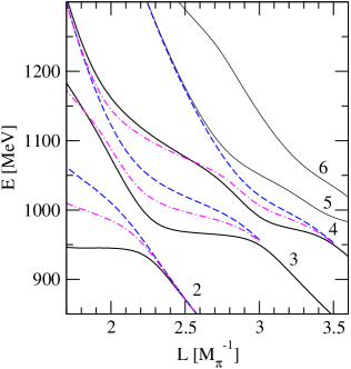
  Figure 3: Solid lines: Spectrum $E(L)$ as in Fig. 1; Dashed lines: Applying twisted b.c. $\theta=\pi$ as in Ref. akaki , only for the $K\bar{K}$ channel and for the levels 2,3, and 4; Dashed dotted lines: with $\theta=\pi/2$.

• Introducing the twisting angle $\theta$ gives us an additional adjustable parameter that allows one to determine the individual matrix elements $V_{ij}$. The same goal can be achieved without twisting, performing the calculations on the asymmetric lattices $L_{x}\times L_{y}\times L_{z}$ where, generally, $L_{x,y,z}$ are not all equal . Note that scattering in an asymmetric box has already been studied on the lattice, see Refs. Li:2007ey ; Liu:2007qq ; Liu2 ; Ishii .

  Suppose $L_{x,y,z}$ have been adjusted so that the value of the energy $E(L_{x,y,z})=E$ stays put. In practice one evaluates the trajectories of the levels, and cuts them by the line of $E=\text{const}$ to determine the $L_{i}$. The loop functions $\tilde{G}_{j}$ depend both on the energy $E$ and the box configuration given by $L_{x,y,z}$. Note that $L^{3}$ in Eq. (15) is now replaced by $L_{x}L_{y}L_{z}$ and $q_{i}=2\pi n_{i}/L_{i}$, $i=1,2,3$, $n_{i}\in\mathds{Z}$. We label the different configurations with the same energy by an index $a=1,2,\cdots$, and denote the pertinent values of the loop functions by $\tilde{G}^{(a)}(E)$. Performing the measurement for three different configurations and solving the secular equation, one can determine the matrix elements of the potential separately,

  $$\left(\begin{array}[]{l}V_{11}\\ V_{22}\\ V_{12}^{2}-V_{11}V_{22}\end{array}\right)=\tilde{G}_{L}^{-1}\left(\begin{array}[]{l}1\\ 1\\ 1\end{array}\right),$$ (24)

  where

  $$\tilde{G}_{L}=\left(\begin{array}[]{lll}\tilde{G}_{1}^{(1)}&\tilde{G}_{2}^{(1)}&\tilde{G}_{1}^{(1)}\tilde{G}_{2}^{(1)}\\ \tilde{G}_{1}^{(2)}&\tilde{G}_{2}^{(2)}&\tilde{G}_{1}^{(2)}\tilde{G}_{2}^{(2)}\\ \tilde{G}_{1}^{(3)}&\tilde{G}_{2}^{(3)}&\tilde{G}_{1}^{(3)}\tilde{G}_{2}^{(3)}\end{array}\right).$$ (28)

  In Fig. 4 we show a particular energy level in the vicinity of 1 GeV, calculated for different configurations of the asymmetric box. It is seen that the level is not very sensitive to the configuration. For this reason, a larger error bar is a priori expected, if observables are extracted from these data.

  

  Figure 4: Energy level 3 in an asymmetric box of dimensions $(L_{x}=L,L_{y}=L,L_{z}=x\,L)$, where $x=0.6$ (solid lines), $x=1.0$ (dashed lines), $x=1.4$ (dash-dotted lines).

  For illustrative purposes, in Fig. 5 we display different physical observables in the $\pi\pi$ and $K\bar{K}$ scattering, that can be extracted from the energy levels by using the above-mentioned methods, no errors yet assigned. As seen, both methods have in principle the capability to address the problem.

  

  

  

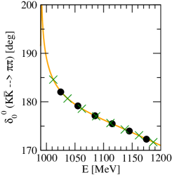
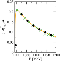
  Figure 5: Left: $\pi\pi\to\pi\pi$ phase shift. Center and right: $K\bar{K}\to\pi\pi$ phase shift and inelasticity. Solid line: infinite-volume phase shift from which the lattice spectrum $E(L)$ is calculated; Crosses (X): Reconstructed phase shift using the twisted b.c. with $\theta=0,\,\pi/2,\,\pi$ of Fig. 3; Solid circles: Using the 3 asymmetric lattice levels of Fig. 4.

For completeness, one should mention that measuring at least 3 different excited levels at the same energy but different values of $L$ could, in principle, also achieve the goal. Such a proposal, however, looks quite unrealistic in the view of the present state of art in the scalar meson sector.

3.3 Threshold effects

At this place, we would like to comment on the threshold effects, which have a capability to seriously complicate the search of the near-threshold resonances – exactly the task we are after. The resonances on the lattice reveal themselves in the form of a peculiar behavior of the volume-dependent energy levels near the resonance energy called “avoided level crossing” Wiese:1988qy . For example, in Fig. 3, the solid curves (levels, corresponding to the periodic b.c.), display a perfect avoided level crossing slightly below 1 GeV. Does this signal the presence of the $f_{0}(980)$?

In order to answer this question, it suffices to change the parameters of the potential slightly, making the $f_{0}(980)$ disappear. This can be achieved, for example, by merely reducing the strength of the potential $V_{11}$ that describes the scattering in the $K\bar{K}\to K\bar{K}$ channel. Namely, replacing $V_{11}\to\eta V_{11}$ and varying $\eta$ between 1 and 0, it is seen that the $f_{0}(980)$ disappears already at $\eta\simeq 0.8$ (the pole moves to a hidden sheet). Below, we shall study the dependence of the energy levels on the parameter $\eta$.

Let us first stick to the periodic b.c. . In the left panel of Fig. 6 one immediately sees that the avoided level crossing in the energy levels persists even for vanishing $\eta$, when there is no trace of the $f_{0}(980)$ any more in the scattering phase (see Fig. 7). This shows very clearly that the avoided level crossing in this case has nothing to do with the $f_{0}(980)$ and is due to the presence of the $K\bar{K}$ threshold. The modified problem has memory of the $K\bar{K}$ channel because the $V_{12}$ term is still kept and connects the two channels.

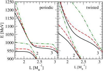
Figure 6: Energy levels, different values of $\eta$. Left panel corresponds to periodic b.c. $\theta=0$, right panel to twisted b.c. $\theta=\pi$. Solid lines: $\eta=1$; Dashed lines: $\eta=0.8$, Dash-dotted lines: $\eta=0$.

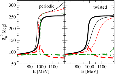
Figure 7: Thick lines: true $\pi\pi$ scattering phases, different values of $\eta$; Thin lines: pseudophases, different values of $\eta$. Left panel corresponds to periodic b.c. $\theta=0$, right panel to twisted b.c. $\theta=\pi$. Solid lines: $\eta=1$; Dashed lines: $\eta=0.8$, Dash-dotted lines: $\eta=0$.

The pseudophase which is displayed in the left panel of Fig. 7 also demonstrates this statement. We see that it barely changes with $\eta\to 0$, whereas the true scattering phase is subject to dramatic changes. A rapid change of the pseudophase by $\pi$ around 1 GeV is related to the presence of the $K\bar{K}$ threshold and not to the $f_{0}(980)$.

Now, the essence of the problem becomes clear. It seems that the presence of the threshold masks the presence of the resonance, and the energy levels become largely insensitive to the latter. How accurate the lattice data should be in order to provide a reliable extraction of the resonance parameters in the vicinity of a threshold?

It should be pointed out that the use of twisted b.c. gives one possible solution to the above problem. Namely, as already mentioned above, as the twisting angle $\theta$ increases, the $K\bar{K}$ threshold moves up, whereas the $f_{0}(980)$ stays put. Consequently, for larger values of $\theta$, these two are well separated, and the pseudophase reveals a larger dependence on the parameter $\eta$. This is demonstrated in the right panels of Figs. 6 and 7.

It remains to be seen, whether the use of twisted b.c. could be advantageous for resolving near-threshold resonances. Below, we address this issue by means of fits to synthetic lattice data.

3.4 The framework based on UCHPT

Finally, we would like to turn to the framework of UCHPT in a finite volume, which is a central issue considered in the present paper. In section 3.2, we did not assume any specific ansatz for the potential $V_{ij}$ which is being extracted from the data. It is clear, however, that, changing the box geometry and/or the twisting angle, we can not arrive exactly to the same energy, and some kind of an interpolation procedure will be needed. This could be achieved by evaluating many points belonging to the same level for different values of $L$ and performing a best fit to the data which will return an accurate trajectory with smaller errors than the individual ones (see, e.g., Refs. Bayes ; Bayes2 ; Chen ) .

Alternatively, one may choose the parameterization of the potential $V_{ij}(E)$ as in UCHPT (e.g., as in Eq. (30) below), and then fitting the parameters of $V_{ij}$ to the data on the lattice introduces certain model-dependence, but provides a fair input based on the successful UCHPT that allows the interpolation of the lattice data. With more lattice data available, $V_{ij}$ as functions of the energy can be fitted more accurately, making the initial ansatz for it less relevant. We would like to stress that the present ansatz for the potential, in our opinion, is simple, rather general and theoretically solid. As mentioned above, it has been successfully used in the past to accurately describe the scattering in the $\pi\pi/\pi\eta$ and $K\bar{K}$ systems (at physical values of the quark masses), see Refs. npa ; Pelaez:2003dy ; Kaiser:1998fi ; Locher:1997gr . This means that the effect of the higher-order terms in the potential should be small. Of course, this assumption could be checked by incorporating such higher order terms as it has been done e.g. in the case of $K^{-}p$ scattering Borasoy:2006sr . It can be expected that, in the first approximation, the functional form of the potential stays intact when we go to higher quark masses that are used in present lattice simulations (the numerical values of the parameters may depend on the quark masses).

Below, performing the fits to the synthetic lattice data with errors, we shall explicitly demonstrate how the approach works.

4 Fit to the energy levels

4.1 Twisted boundary conditions versus asymmetric boxes

Below, we shall carry out a preliminary numerical estimate of the efficiency of the two different schemes which were discussed above. To this end, first we produce the energy levels by using UCHPT in a finite volume. Then we assume that each data point $E(L)$ is produced with some uncertainty $\Delta E(L)$. Reversing the dependence on $L$, one obtains $L(E)$ and $\Delta L(E)$ (in case of an asymmetric box we have taken $L_{i}=\alpha_{i}\,L$ for three different choices of $\alpha_{i}$ and we take the same $\Delta L$ as in the symmetric case). In general, for a given $E(L)$ and $\Delta E(L)$, the inverse $\Delta L(E)$ is a very complicated function of energy, depending on the tangent of the curve. Since we are making only a rough estimate here, we simplify our task by assuming a constant error $\Delta L=0.02M_{\pi}^{-1}$. Further, using the von Neumann rejection method, we generate a Gaussian distribution for the variable $L$ centered around the exact solution $a=L(E)$

$$f(L)=\frac{1}{\Delta L\sqrt{2\pi}}\exp\left\{-\frac{(L-a)^{2}}{2(\Delta L)^{2}}\right\}\,.$$ (29)

We perform the calculations of the infinite-volume phase shifts for each value of $L$ and determine the average value and uncertainty, using Eq. (24). The results for two different methods are shown in Fig. 8.

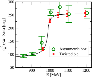
Figure 8: Error estimates for two different extraction schemes.

Below and above the $K\bar{K}$ threshold, both methods deliver very similar phase shifts with a comparable error. Around the $K\bar{K}$ threshold, as expected, the use of twisted b.c. produces phase shifts with an error smaller than in the other method.

4.2 Extraction of the $f_{0}(980)$ pole position from the data

After the preliminary study of the different schemes carried out in the previous subsection, we turn to the main topic of our paper and perform the fit of the data by using UCHPT in a finite volume. To this end, we consider the procedure for producing various synthetic data sets and the strategy of the fit.

The central values $E_{n}(L),~{}n=0,1,\cdots$ are produced by solving the secular equation (17) with the potentials from UCHPT, by using periodic/antiperiodic b.c. (below, we do not study the case of the asymmetric boxes). At the next step, a constant error $\Delta E=10~{}\mbox{MeV}$ is assigned to each of the data points. We consider three different data sets in the vicinity of the $f_{0}(980)$, each of them containing 13 data points (see Fig: 9):

1. The data set from the levels 2 and 3, using periodic b.c.

2. The level 2, using both periodic and antiperiodic b.c. As we shall see, the use of the twisted b.c. enables one to achieve a better accuracy than in set 1.

3. The levels 2 and 3, periodic b.c., modified input (the parameter $\eta=0.6$, so the $f_{0}(980)$ pole is absent). As seen from Fig. 9, there is no qualitative change of behavior of the energy levels in sets 1 and 3. It is important to check, whether the method is capable to distinguish between these two cases.

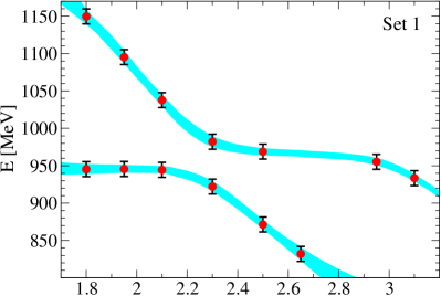
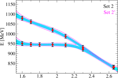
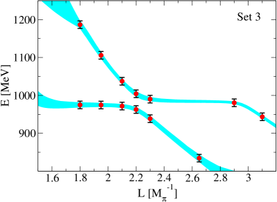
Figure 9: Generated data points (10 MeV error, 13 points for each set). Upper figure: using levels 2 and 3 with periodic b.c.; Central figure: using level 2 with periodic and antiperiodic b.c.; Lower figure: case without $f_{0}(980)$ (using levels 2,3 with periodic b.c.). Fits that fulfill the $\chi_{\rm best}^{2}+1$ criterion are also shown in all figures [solid (cyan) bands]. The set $2^{\prime}$ corresponds to data with displaced centroids (see Sec. 4.3 for more details). In the central figure, the fits to set $2^{\prime}$ are shown by dashed lines and the hatched (magenta) bands.

Further, for each set the data $E_{i}(L)$ shown in Fig. 9 are fitted by using linear functions in the potential $V_{ij}$,

$$V_{ij}=a_{ij}+b_{ij}(s-4M_{K}^{2})\,$$ (30)

which is used to calculate $E^{\rm(theory)}_{i}(L)$ by using Eq. (17). The six parameters of the potential $a_{ij}$ and $b_{ij}$ are assumed to be free and are determined from the fit to the spectrum. Note that, since the input potential which was used to produce the data points is also linear in $s$, the $\chi^{2}$-value of the best fit is equal to 0.

To obtain the error on the extracted quantities (phase shifts and pole positions), random $a_{ij},\,b_{ij}$ are generated within the limits given by the parameter errors, that are determined by the previous fit. Of these combinations, only those are accepted for which the resulting $\chi^{2}$ is smaller than $\chi_{\rm best}^{2}+1$. For each such event, the $\pi\pi$ phase is evaluated and the pole position in the complex energy plane is determined. The resulting bands for the phase shifts and extracted pole positions are shown in Figs. 10 and 11.

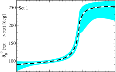
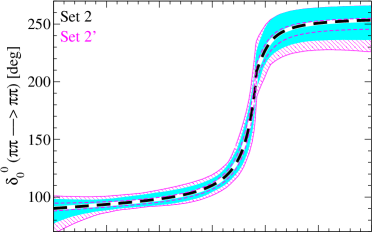
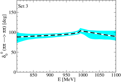
Figure 10: Extracted phase shifts corresponding to the three sets shown in Fig. 9. Dashed lines: The calculated phase shifts by using the approach of Ref. npa ; Filled (cyan) bands: Reconstruction of these phase shifts.

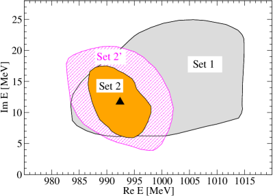
Figure 11: Extracted pole positions. Filled triangle: original pole position npa ; Shapes: Pole positions reconstructed from the data sets 1, 2, and $2^{\prime}$, see Fig. 9. For the data set 3, the poles are found either on the hidden sheets, or very far from the $K\bar{K}$ threshold.

From these figures one observes that, for all fits to the synthetic data with $f_{0}(980)$ (sets 1,2), which obey the $\chi_{\rm best}^{2}+1$ criterion, the phase shift shows a resonant behavior and a pole is found in the complex plane on the first $K\bar{K}$ sheet (second sheet for the $\pi\pi$ channel). Also, in all fits to data without $f_{0}(980)$ (set 3), the phase shifts show no resonant behavior, and no pole is found in the vicinity of the $K\bar{K}$ threshold — the poles are in this case on a hidden sheet far from the physical region. Thus, with the method proposed here, it is indeed possible to distinguish clearly the presence or absence of a resonance at the $K\bar{K}$ threshold.

Moreover, as the figures 10 and 11 show, using 13 data points with a 10 MeV error, the pole position of the $f_{0}(980)$ can be determined quite precisely. As seen in Fig. 11, the data set 2 gives a more precise determination of the pole position than the data set 1: it is advantageous to use data from a lower level but with different boundary conditions, than to use the data from higher excited levels.

If fewer lattice data are included in the analysis than those of Fig. 9, the six-parameter fit is less constrained. Then, the spread in extracted pole positions and phase shifts can increase. This is reflected in a blow-up of the bands shown in Fig. 9, in regions without data. Then, adding a data point precisely in this region helps constrain the fit. In an actual lattice calculation, such observations could help to guide the selection of lattice sizes $L$ for which the levels are calculated.

4.3 Statistical scattering of the data (Set $2^{\prime}$)

In an actual lattice simulation the finite statistics will not only contribute to the error bar of a data point but also lead to a displacement of its centroid. To study this effects, we concentrate on data set 2 and choose a Gaussian distribution with $\sigma=5$ MeV for the displacement of the centroids. Using Eq. (29) for every data point, 13 new points for Set 2 are generated and then fitted. The resulting fit leads to a slightly modified pole position and phase shift. To obtain, however, reliable results, this procedure has to be repeated multiple times. The multiple generated data sets are called Set $2^{\prime}$ in the following. To obtain confidence regions for levels and phase shifts, the multiple fits to Set $2^{\prime}$ are analyzed. For example, for the resulting phase shifts, at every energy $E$ the mean value and standard deviation for all fits are calculated. The resulting band is indicated with the dashed lines in Fig. 10. The same can be made for the levels themselves as indicated with the dashes lines in Fig. 9.

To estimate the combined effect of uncertainty from the previously discussed $\chi_{\rm best}^{2}+1$-criterion and displaced centroids, we calculate the average $\chi_{\rm ave}^{2}$ from the multiple fits to set $2^{\prime}$, with the result $\chi_{\rm ave}^{2}\sim 1.7$. The overall uncertainty is then estimated from applying a $\chi_{\rm best}^{2}+\chi_{\rm ave}^{2}+1$-test on set 2, i.e. the data set without displaced centroids. The resulting bands are indicated with the hatched areas in Figs. 9 and 10. As expected, their widths is approximately given by the sum of widths from the $\chi_{\rm best}^{2}+1$-criterion [solid (cyan) areas] plus the 1-$\sigma$ region of the multiple fits to set $2^{\prime}$ [dashed lines]. In Fig. 11, the combined uncertainty for the pole position is shown [hatched area]. In summary, we observe that the scattering of the centroids leads to a moderate increase of the uncertainties for levels, phases and pole positions. With a Gaussian distribution of 5 MeV width for the displacement of the centroids, the uncertainties induced by 10 MeV error bars are increased by maximally 50 %.

4.4 Systematic uncertainties

A comprehensive treatment of systematic uncertainties would require to address the actual lattice action that generates the levels, but that is far beyond of what can be possibly done in the present framework. What can be studied, however, is the scenario when the chosen fit potential cannot achieve a perfect fit of the lattice data. As mentioned above, the choice of the potential of Eq. (30) replicates the lowest-order chiral interaction that has been used to generate the synthetic data. To test the more realistic situation, in which the lattice data can not be perfectly fitted, apart from the statistical scattering of the data discussed in the previous section, we introduce a small term $\sim c_{ij}\,(s-4M_{K}^{2})^{2}$ in the potential that is used to generate the synthetic data. The constants $c_{ij}$ are chosen to be $c_{11}=c_{22}=-c,~{}c_{12}=c_{21}=+c$ where $c=310.8~{}\mbox{GeV}^{-4}$. The effect of introducing this term on the phase $\delta_{0}^{0}$ and on the energy spectrum (periodic b.c.) is seen in Fig. 12. The fit to the modified data points (squares in Fig. 12) and subsequent analysis are then performed using the same potential as before, i.e. Eq. (30).

 

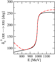
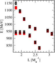
Figure 12: The effect of introducing the quadratic term proportional to $c_{ij}$, on the scattering phase $\delta_{0}^{0}$ (left panel), and on the energy spectrum (right panel). The solid curve and the circles correspond to $c_{ij}=0$. The dashed line on the left-hand side and the squares on the right-hand side correspond to $c_{ij}\neq 0$ (small quadratic term in the potential, see text).

The resulting $\chi^{2}_{\rm best}$ does not vanish any more, and the extracted pole positions and phases are systematically shifted as shown in Fig. 13, case (a) and (b) (the latter correspond to data sets 1 and 2 in Fig. 9. In addition, to make these areas distinguishable, we have assigned an error $\Delta E=5~{}\mbox{MeV}$ in case (a), instead of 10 MeV.).

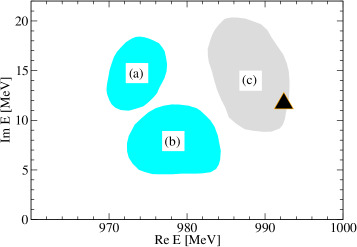
Figure 13: Systematic errors. Large triangle: Actual pole position; (a), (b): effect of slightly shifted lattice data points (cf. Fig. 12) on the reconstructed pole position, for the data sets 1 and 2 shown in Fig. 9; (c): Cut-off-dependence ($q_{\rm max}=755$ MeV instead of $904$ MeV as used in the generation of the data).

This kind of systematic error is inherently tied to the assumption made on the functional form of the potential (cf. Eq. (30)): one could, of course, introduce higher order terms in the potential to extract phase shifts and pole positions. Then, $\chi^{2}_{\rm best}$ would be close to zero again, but the fit would be much less constrained given the higher number of free parameters. The spread of pole positions and extracted phases would then immediately increase as compared to the present results. Still, it would be worth to quantify the effects of the higher order terms on the accuracy of these determinations in future studies.

Apart from the discussed higher order terms for the potential $V$, another source of uncertainty is given by the cutoff $q_{\rm max}$ that is used to determine phase shifts and pole positions once the $V_{ij}$ are fitted: the term $\tilde{G}$ of Eq. (17) depends on this $q_{\rm max}$. To test the dependence, we have extracted the pole positions with $q_{\rm max}=755$ MeV instead of using the standard value of $904$ MeV that has been used to generate the synthetic data. The result is shown as case (c) in Fig. 13. Obviously, the functional form of Eq. (30) in $V_{ij}$ is flexible enough to compensate for this large change in $q_{\rm max}$ and as a result the pole position is shifted by just a few MeV. Systematic effects from the cut-off dependence are, thus, very small.

We have made another test which can be of use if one could make a rough estimate of the size of the systematic uncertainties of the lattice results. Systematic uncertainties would most likely produce deviations of the energy levels in the same direction. We have assumed a constant shift of the energy levels, increasing them by 5 MeV, and we have found a decrease of about 5% in the phase shifts, and viceversa.

To summarize, a careful examination of all kind of errors has been carried out in this subsection, illustrating the limitations of the proposed method. Given only a few lattice data with large error, UCHPT in finite volume is certainly a useful tool to make reliable statements on the presence or absence of resonances, and even to give a good first estimate on phases and pole positions.

4.5 The $a_{0}(980)$

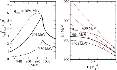
Figure 14: Left: lineshapes in $\pi\eta\to\pi\eta$. Note that the $a_{0}$ shows a true resonance pole for $q_{\rm max}=1094$ MeV, while for $q_{\rm max}=904$ and $630$ MeV, it is rather a cusp at the $K\bar{K}$ threshold than a resonance (in this case, the pole is on a hidden sheet); Right: Level 1 for three different cutoffs $q_{\rm max}=1094,\,904,\,630,$ MeV, with periodic (solid, dashed, dash-dotted) and antiperiodic (dotted) b.c.

The situation concerning the $a_{0}(980)$ in UCHPT is intriguing. For example, in Ref. npa , the $a_{0}(980)$ is generated from the lowest order chiral Lagrangian in the $\pi\eta$ and $K\bar{K}$ channels. At present, there exists no consensus about its nature and exact location. For example, changing the cutoff $q_{\rm max}$ in the approach of Ref. npa , one may easily move the pole below/above the $K\bar{K}$ threshold. Namely, for $q_{\rm max}=1094$ MeV, the pole of the $a_{0}$ is below the $K\bar{K}$ threshold and one observes the full resonance shape (see the left panel of Fig. 14). For lower cut-offs, say $q_{\rm max}=904$ MeV and $q_{\rm max}=630$ MeV, the pole disappears from the second Riemann sheet and instead of a resonance shape, a pronounced threshold cusp structure is visible. This was already observed in Refs. npa ; Oller:1998hw .

This is an interesting situation, because there are several examples in the literature where it is not clear if an observed structure is a resonance or rather a cusp (example: a disputed pentaquark in $\gamma n\to\eta N$ Kuznetsov:2007gr ; Shklyar:2006xw ; Doring:2009qr ; Anisovich:2008wd ). Using UCHPT in a finite volume, one may predict the dependence of the energy levels on the cutoff parameters and see, whether there is a clear-cut distinction between the situations with a resonance or a cusp.

In order to show how the different scenarios influence the energy levels in the box, we carry out the calculation and show the results in Fig. 14. In the left panel of this figure we show the lineshapes in $\pi\eta\to\pi\eta$ for three different cutoffs. In the right panel, we display the energy level 1 for the same values of the cutoff, both for periodic and antiperiodic b.c. As one observes from this plot, the level is quite sensitive to the value of the cutoff. Consequently, it is expected that the extraction of the pole position from future lattice data can be performed accurately, resulting in a clear-cut resolution of the resonance/cusp scenario.

4.6 The $f_{0}(600)$

  

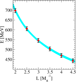
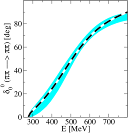
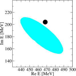
Figure 15: Left: Synthetic lattice data (with errors) for the energy level 1; Center: The extracted phase shift vs the original $\delta_{0}^{0}$ phase shift (dashed line); Right: The spread in the pole positions. The filled circle shows the original pole position.

It comes rather as a surprise that the procedure seems to work even in case of the $f_{0}(600)$. In order to do this, we have resorted to the 1-channel Lüscher formalism, because the energy is well below the $K\bar{K}$ threshold. Only the level 1 with periodic b.c. was fitted (see Fig. 15, left panel). The fit resulted in the phase shifts shown in the center panel and in the pole positions displayed in the right panel of the same figure. As seen from the figure, the spread in pole positions is larger than in case of $f_{0}(980)$, but, in our opinion, it is remarkable that one is able to address the question of the extraction of the $f_{0}(600)$ on the lattice at all. Note also that, as seen from Fig. 15, the small effect of the sub-threshold $K\bar{K}$ channel is visible in the extracted phase for the highest energies above 600 MeV. Also, for the same reason, there is an off-set between the true pole position (dark circle, right-hand panel) and the extracted ones (large shaded area). To verify this, we have generated pseudo data using only the $\pi\pi$-channel in the hadronic model npa . Then, extracting pole positions with the one-channel formalism, the resulting ellipse should have the true pole position (of the $\pi\pi$-reduced hadronic model) in its center. This is indeed the case as has been checked.

The $f_{0}(600)$ (or $\sigma$) has been predicted in most UCHPT approaches (see, e.g., Refs. npa ; Locher:1997gr ; Oller:1998hw ). Recently, its existence has been rigorously proved by using ChPT combined with Roy equations Caprini:2005zr . It would be intriguing, if the already existing lattice studies of the lowest scalar resonance in QCD Mathur:2006bs ; Kunihiro:2003yj ; Prelovsek:2010gm could be supplemented by the novel method of the analysis based on UCHPT, in order to facilitate the extraction of the pole position in the complex plane.

5 Conclusions

In this paper, we discuss the extraction of the parameters of the $f_{0}(600)$, $f_{0}(980)$ and $a_{0}(980)$ resonances from lattice data. In order to facilitate this extraction, we use UCHPT in a finite volume in the fit. Fitting synthetic data, we have demonstrated that the approach works, and the pole position for the above resonances can indeed be extracted by analyzing the volume-dependent energy spectrum in the vicinity of the resonance energy, provided sufficiently many volumes are simulated. The different sources of errors are analyzed in detail. The key point is that the use of the phenomenological input from UCHPT stabilizes the fit. It is, thus, very challenging to apply these results to present and forthcoming lattice data in order to extract valuable information concerning hadronic resonances. From the theoretical point of view one should also keep in mind that in field theory there are parts of the kernel of the Bethe-Salpeter equation which are volume dependent, although exponentially suppressed. Quantitative studies of these terms and the extent of the large $L$ suppression would be a very good complement to the work we have carried out here.

Appendix A Quantitative comparison to the Lüscher approach

As we have seen in Sec. 2.2, the connection of our approach with the Lüscher approach comes through the replacement $\tilde{G}_{j}(E)\to\tilde{G}_{jA}(E)$, where

$$\tilde{G}_{jA}(E)-G_{j}(E) = -\frac{1}{4\pi^{3/2}EL}\,{\cal Z}_{00}(1;\hat{p}^{2})$$ (31)

$$+ \frac{i}{16\pi E^{2}}\,\lambda^{1/2}(E^{2},m_{1}^{2},m_{2}^{2})\,.$$

It is straightforward to see that, substituting $G$ in Eq. (1) by $\tilde{G}_{jA}$ of Eq. (31), one arrives at the two-channel Lüscher equation from Ref. akaki , which is written in terms of the $K$-matrix.

Next we discuss the differences of the functions $\tilde{G}_{j}(E)$ of Eq. (15) and $\tilde{G}_{jA}(E)$. In Fig. 16 we show the results for two different values of $L$ for the $\pi\pi$ and the $K\bar{K}$ channels.

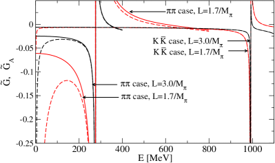
Figure 16: Comparison of $\tilde{G}_{j}(E)$ of Eq. (15) [solid lines] and $\tilde{G}_{jA}(E)$ of Eq. (31) [dashed lines], for the $\pi\pi$ and $K\bar{K}$ channels. Two cases for $L=1.7/M_{\pi}$ and $L=3.0/M_{\pi}$ are shown.

We can see that for the $\pi\pi$ channel the differences for $L=1.7\,M_{\pi}^{-1}$ are rather large for energies below 250 MeV, which is already below the $\pi\pi$ threshold. Even above threshold, the differences are sizable. These differences are smaller for a bigger $L$, $L=3.0\,M_{\pi}^{-1}$, as expected for exponentially suppressed terms. In both cases the function $\tilde{G}_{jA}(E)$ has a pole at $E=0$, while $\tilde{G}_{j}(E)$ is finite there. For the case of the $K\bar{K}$ channel, the trend is similar to the $\pi\pi$ channel, but the region where $\tilde{G}_{jA}(E)$ and $\tilde{G}_{j}(E)$ are practically equal is larger than in the $\pi\pi$ case.

It is interesting to see, how big the effect of this difference is on the energy levels in the box. This is seen in Fig. 17, left panel.

  

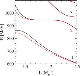
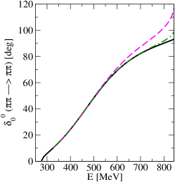
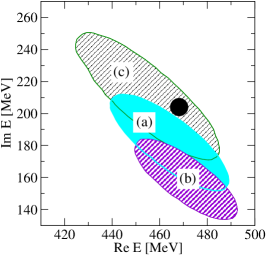
Figure 17: Left panel: Levels obtained with $\tilde{G}_{j}(E)$ of Eq. (15) [solid lines, identical to Fig. 1] and with $\tilde{G}_{jA}(E)$ of Eq. (31) [dashed lines]. Center panel, dashed and dash-dotted lines: Pseudophases (one-channel formalism) obtained from the levels shown in the left panel [see text], using Eq. (2.1). Solid line: Original phase. Right panel: Pole positions for $f_{0}(600)$, extracted by using the method of section 4.6. For cases (a), (b), (c), see text.

As we see from Fig. 17, left panel, if $L\geq 1.6\,M_{\pi}^{-1}$, the corrections to the energy levels 2,3,…are completely negligible. Therefore, we concentrate on level 1 where the difference between the solid and dashed curves can not be neglected. We calculate the $\pi\pi$ pseudophases, see Fig. 17, central panel, and the position of the poles of the $f_{0}(600)$ corresponding to these two curves, see Fig. 17, right panel .

As one sees from Fig. 17, the pseudophases are fairly the same until 500 MeV, from where they start diverging. At $L=2\,M_{\pi}^{-1}$ that corresponds to $E\simeq 700~{}\mbox{MeV}$, the difference between two pseudophases is around 5 degrees. If the energy grows (the volume decreases), the difference between the two pseudophases becomes, as expected, bigger.

In Fig. 17, right panel, we display the shift of the pole positions due to the effect of using the relativistic propagator. The same method as in section 4.6 was used to produce the ellipses. Case (a) shows the pole positions extracted from levels generated using the relativistic propagator (identical case to the one shown in Fig. 15). In case (b) the pole positions have been extracted from the level generated with $\tilde{G}_{jA}(E)$ of Eq. (31), i.e. from the dashed curve shown in the left panel. As we see, the real part of the pole undergoes a shift of order of 10 MeV, whereas the width (twice the imaginary part of the pole position) changes by approx. 40 MeV.

As we see, the uncertainty of the method which stems from the error of 10 MeV in energy attached to each data point, is still larger than the change induced by the use of the relativistic propagators. Should one aim at an accuracy of better than 40 MeV in the width, first, the errors in the lattice data should improve beyond 10 MeV and, second, from our study it follows that the standard Lüscher approach is not accurate enough in this case.

So far, we were concerned how a shift in the level translates into a shift of the pseudophase and pole position; one may also ask what happens if $\tilde{G}_{jA}(E)$ of Eq. (31) is used to extract the pole position from a given level, instead of using the relativistic propagator $\tilde{G}_{j}(E)$ of Eq. (15) as done before. The effect is shown as case (c) in the right-hand panel of Fig. 17. Compared to case (a), one observes a systematic shift of the results, which is of similar size as the previously discussed case (b).

References

- (1) Y. Nakahara, M. Asakawa, T. Hatsuda, Phys. Rev. D60 (1999) 091503 [arXiv:hep-lat/9905034].
- (2) K. Sasaki, S. Sasaki and T. Hatsuda, Phys. Lett. B 623 (2005) 208 [arXiv:hep-lat/0504020].
- (3) N. Mathur, A. Alexandru, Y. Chen et al., Phys. Rev. D76 (2007) 114505 [arXiv:hep-ph/0607110].
- (4) S. Basak, R. G. Edwards, G. T. Fleming et al., Phys. Rev. D76 (2007) 074504 [arXiv:0709.0008 [hep-lat]].
- (5) J. Bulava, R. G. Edwards, E. Engelson et al., Phys. Rev. D82 (2010) 014507 [arXiv:1004.5072 [hep-lat]].
- (6) J. J. Dudek, R. G. Edwards, B. Joo, M. J. Peardon, D. G. Richards, C. E. Thomas, Phys. Rev. D83 (2011) 111502 [arXiv:1102.4299 [hep-lat]].
- (7) C. Morningstar, A. Bell, J. Bulava et al., AIP Conf. Proc. 1257 (2010) 779 [arXiv:1002.0818 [hep-lat]].
- (8) J. Foley, J. Bulava, K. J. Juge et al., AIP Conf. Proc. 1257 (2010) 789 [arXiv:1003.2154 [hep-lat]].
- (9) R. Baron et al. [ ETM Collaboration ], JHEP 1008 (2010) 097 [arXiv:0911.5061 [hep-lat]].
- (10) M. G. Alford and R. L. Jaffe, Nucl. Phys. B 578 (2000) 367 [arXiv:hep-lat/0001023].
- (11) T. Kunihiro, S. Muroya, A. Nakamura, C. Nonaka, M. Sekiguchi and H. Wada [SCALAR Collaboration], Phys. Rev. D 70 (2004) 034504 [arXiv:hep-ph/0310312].
- (12) F. Okiharu et al., arXiv:hep-ph/0507187.
- (13) H. Suganuma, K. Tsumura, N. Ishii and F. Okiharu, PoS LAT2005 (2006) 070 [arXiv:hep-lat/0509121].
- (14) H. Suganuma, K. Tsumura, N. Ishii and F. Okiharu, Prog. Theor. Phys. Suppl. 168 (2007) 168 [arXiv:0707.3309 [hep-lat]].
- (15) C. McNeile and C. Michael [UKQCD Collaboration], Phys. Rev. D 74 (2006) 014508 [arXiv:hep-lat/0604009].
- (16) A. Hart, C. McNeile, C. Michael and J. Pickavance [UKQCD Collaboration], Phys. Rev. D 74 (2006) 114504 [arXiv:hep-lat/0608026].
- (17) H. Wada, T. Kunihiro, S. Muroya, A. Nakamura, C. Nonaka and M. Sekiguchi, Phys. Lett. B 652 (2007) 250 [arXiv:hep-lat/0702023].
- (18) S. Prelovsek, C. Dawson, T. Izubuchi, K. Orginos and A. Soni, Phys. Rev. D 70 (2004) 094503 [arXiv:hep-lat/0407037].
- (19) S. Prelovsek, T. Draper, C. B. Lang, M. Limmer, K. F. Liu, N. Mathur and D. Mohler, arXiv:1002.0193 [hep-ph].
- (20) S. Prelovsek, T. Draper, C. B. Lang, M. Limmer, K. F. Liu, N. Mathur and D. Mohler, arXiv:1005.0948 [hep-lat].
- (21) M. Lüscher, Commun. Math. Phys. 105 (1986) 153 (1986).
- (22) M. Lüscher, Nucl. Phys. B 354 (1991) 531.
- (23) C. Liu, X. Feng and S. He, Int. J. Mod. Phys. A 21 (2006) 847 [arXiv:hep-lat/0508022].
- (24) M. Lage, U.-G. Meißner and A. Rusetsky, Phys. Lett. B 681 (2009) 439 [arXiv:0905.0069 [hep-lat]].
- (25) V. Bernard, M. Lage, U.-G. Meißner and A. Rusetsky, JHEP 1101 (2011) 019 [arXiv:1010.6018 [hep-lat]].
- (26) J. A. Oller, E. Oset, Nucl. Phys. A620 (1997) 438 [Erratum-ibid. A 652 (1999) 407] [arXiv:hep-ph/9702314].
- (27) J. R. Pelaez, Phys. Rev. Lett. 92 (2004) 102001 [arXiv:hep-ph/0309292].
- (28) N. Kaiser, Eur. Phys. J. A3 (1998) 307.
- (29) M. P. Locher, V. E. Markushin, H. Q. Zheng, Eur. Phys. J. C4 (1998) 317 [arXiv:hep-ph/9705230].
- (30) V. Bernard, M. Lage, U.-G. Meißner and A. Rusetsky, JHEP 0808 (2008) 024 [arXiv:0806.4495 [hep-lat]].
- (31) A. M. Torres, L. R. Dai, C. Koren, D. Jido, E. Oset, [arXiv:1109.0396 [hep-lat]].
- (32) M. Döring, J. Haidenbauer, U.-G. Meißner, A. Rusetsky, [arXiv:1108.0676 [hep-lat]].
- (33) J. Gasser and H. Leutwyler, Annals Phys. 158 (1984) 142.
- (34) E. Oset and A. Ramos, Nucl. Phys. A 635 (1998) 99 [arXiv:nucl-th/9711022].
- (35) J. A. Oller and E. Oset, Phys. Rev. D 60 (1999) 074023 [arXiv:hep-ph/9809337].
- (36) J. A. Oller and U.-G. Meißner, Phys. Lett. B 500 (2001) 263 [arXiv:hep-ph/0011146].
- (37) S. R. Beane, P. F. Bedaque, A. Parreno et al., Nucl. Phys. A747 (2005) 55 [arXiv:nucl-th/0311027].
- (38) J. Yamagata-Sekihara, J. Nieves, E. Oset, Phys. Rev. D 83 (2011) 014003 [arXiv:1007.3923 [hep-ph]].
- (39) D. Gamermann, J. Nieves, E. Oset and E. Ruiz Arriola, Phys. Rev. D 81 (2010) 014029 [arXiv:0911.4407 [hep-ph]].
- (40) X. Li et al. [CLQCD Collaboration], JHEP 0706 (2007) 053 [arXiv:hep-lat/0703015].
- (41) C. Liu, X. Feng and S. He, Int. J. Mod. Phys. A 21 (2006) 847 [arXiv:hep-lat/0508022].
- (42) C. Liu et al., PoS LAT2007 (2007) 121 [arXiv:0710.1464 [hep-lat]].
- (43) N. Ishii and HAL QCD Collaboration, arXiv:1102.5408 [hep-lat].
- (44) U. J. Wiese, Nucl. Phys. Proc. Suppl. 9 (1989) 609.
- (45) M. Asakawa, T. Hatsuda and Y. Nakahara, Prog. Part. Nucl. Phys. 46 (2001) 459 [arXiv:hep-lat/0011040].
- (46) G. P. Lepage, B. Clark, C. T. H. Davies, K. Hornbostel, P. B. Mackenzie, C. Morningstar and H. Trottier, Nucl. Phys. Proc. Suppl. 106 (2002) 12 [arXiv:hep-lat/0110175].
- (47) Y. Chen et al., arXiv:hep-lat/0405001.
- (48) B. Borasoy, U.-G. Meißner and R. Nissler, Phys. Rev. C 74 (2006) 055201 [arXiv:hep-ph/0606108].
- (49) J. A. Oller, E. Oset, J. R. Pelaez, Phys. Rev. D59 (1999) 074001 [arXiv:hep-ph/9804209].
- (50) V. Kuznetsov et al. [GRAAL Collaboration], Phys. Lett. B 647 (2007) 23 [arXiv:hep-ex/0606065].
- (51) V. Shklyar, H. Lenske and U. Mosel, Phys. Lett. B 650 (2007) 172 [arXiv:nucl-th/0611036].
- (52) M. Döring and K. Nakayama, Phys. Lett. B 683 (2010) 145 [arXiv:0909.3538 [nucl-th]].
- (53) A. V. Anisovich, I. Jaegle, E. Klempt, B. Krusche, V. A. Nikonov, A. V. Sarantsev and U. Thoma, Eur. Phys. J. A 41 (2009) 13 [arXiv:0809.3340 [hep-ph]].
- (54) I. Caprini, G. Colangelo and H. Leutwyler, Phys. Rev. Lett. 96 (2006) 132001 [arXiv:hep-ph/0512364].