Searching for dark matter isocurvature initial conditions with N-body Simulations

Abstract

Small fraction of isocurvature perturbations may exist and correlate with adiabatic perturbations in the primordial perturbations. Naively switching off isocurvature perturbations may lead to biased results. We study the effect of dark matter isocurvature on the structure formation through N-body simulations. From the best fit values, we run four sets of simulation with different initial conditions and different box sizes. We find that, if the fraction of dark matter isocurvature is small, we can not detect its signal through matter power spectrum and two point correlation function with large scale survey. However, the halo mass function can give an obvious signal. Compared to $5\%$ difference on matter power spectrum, it can get $37\%$ at $z=3$ on halo mass function. This indicates that future high precise cluster count experiment can give stringent constraints on dark matter isocurvature perturbations.

I introduction

Recent high accuracy observations, such as cosmic microwave background radiation (CMB)wmap7 , and the large scale structure (LSS)sdss , provide us wealthy information on the universe. Currently, so called concordance cosmological model, in which approximately scale-invariant, Gaussian, adiabatic primordial perturbations seed the structure of our universe, is mostly favored. However, there exist some models which predict non-negligible isocurvature perturbations, such as multiple scalar fields inflationLiddle:1998jc ; Kanti:1999vt ; Copeland:1999cs ; Langlois:1999dw ; Wands:2002bn ; Piao:2002vf ; Dimopoulos:2005ac ; Langlois:2008wt ; Cai:2009hw ; Cai:2008if ; Cai:2010wt and curvatonLyth:2001nq ; Moroi:2001ct ; Lyth:2002my models. The primordial isocurvature perturbations then can induce the cosmological matter perturbations such as cold dark matter (CDM), baryons, dark energy and neutrinoSeckel:1985tj ; Linde:1991km ; Linde:1996gt ; Liu:2010ba in the radiation era.

Although the pure isocurvature perturbations have already been ruled out by the observation of Boomerang and MAXIMA-1Enqvist:2000hp , models with primordial perturbations comprised of dominate adiabatic and a small fraction of isocurvature modesGordon:2002gv ; Crotty:2003rz ; Bucher:2004an ; Moodley:2004nz ; KurkiSuonio:2004mn ; Beltran:2005xd ; Bean:2006qz ; Trotta:2006ww ; Sollom:2009vd ; Valiviita:2009bp ; Beltran:2005gr ; Mangilli:2010ut ; Li:2010yb still survive. Due to the quality of data, we still can not confirm the destiny of the isocurvature perturbation. Moreover, if we switch off the isocurvature perturbations naively, the result would be misleadingZunckel:2010mm ; Liu:2010ba . So, it is important to seek a way to detect the isocurvature perturbations and give stringent constraints on isocurvature perturbations parameters.

In Ref. Li:2010yb , we have given constraints on parameters of two different cosmological models with latest astronomical data. One is with pure adiabatic initial condition (IC) and the other is with mixed IC in which small fraction of isocurvature mode is correlated with dominating adiabatic mode through $\cos\Delta$. We found that compared to adiabatic mode, the isocurvature perturbations have smaller amplitude ($A_{s}^{iso}/A_{s}^{adi}\sim 10^{-2}$) and bluer tilt ($n_{s}^{iso}\sim 2$). That is to say the isocurvature modes is pronounced on small scales ($k>1~{}\text{h}~{}\text{Mpc}^{-1}$). However, on these scales, the structure grows non-linearly, so we can not study the details of evolution in a full analytical way and then test them against future high-precision observations.

On the other way, N-body simulations plays more and more important role in cosmology nowadays, especially in the study of nonlinearity. It can make predictions and compare with observations for a specific model. It can also be used to check the validity of a particular method Bagla:2004au .

In this work, we study the effects of CDM isocurvature perturbations on LSS by implementing N-body simulations. Given the best fit parameters in Ref. Li:2010yb , we carry out four sets of simulations with different ICs in different boxes. We find that, unlike the power spectrum and two point correlation function, mass function is sensitive to dark matter isocurvature perturbations. This indicates that, we can give stringent constraints on dark matter isocurvature perturbations with future high precision cluster counts experiment.

The structure of this paper is organized as follows. In Sec. II, we briefly introduce the CDM isocurvature perturbation and set the ICs for N-body simulation. In Sec. III, we describe the details of our N-body simulation and present the result. We give summary in Sec. IV.

II Correlated adiabatic and isocurvature perturbations

Generally, to calculate matter power spectra $P(k)$ numerically, one start from the time $t_{ic}$ deep in the radiation dominated era, when all interesting scales of perturbations are outside the horizon. However, $t_{ic}$ is different from the time $t_{*}$ when the corresponding mode $k$ exits horizon during inflation. Therefore, One need transfer function $T_{ij}$ to transform perturbations from $t_{*}$ to $t_{ic}$.

As we know, in the absence of isocurvature perturbations, the adiabatic perturbations $\mathcal{R}$ are conserved on superhorizon scales. On the contrary, the isocurvature perturbations $\mathcal{S}$ can evolve on superhorizon scale and can also seed adiabatic perturbations. Thus, the transfer function $T_{ij}$ can be written asAmendola:2001ni

$$\begin{bmatrix}\mathcal{R}(t_{ic})\\ \mathcal{S}(t_{ic})\end{bmatrix}=\begin{bmatrix}1&T_{\mathcal{RS}}\\ 0&T_{\mathcal{SS}}\end{bmatrix}\begin{bmatrix}\mathcal{R}(t_{*})\\ \mathcal{S}(t_{*})\end{bmatrix},$$ (1)

where $T_{ij}$ is model dependent. To investigate isocurvature perturbation without making use of any specific model, one often parametrizes the transfer function in the simple form of power law.

For the Gaussian statistics, which is predicted by inflation, the power spectra characterize all the information.

$$\mathcal{P}_{ij}\equiv\frac{k^{3}}{2\pi^{2}}\langle\mathcal{X}_{i}({\bf k})\mathcal{X}_{j}({\bf k}^{\prime})\rangle\delta({\bf k}-{\bf k}^{\prime}),$$ (2)

where $\mathcal{X}_{1}=\mathcal{R}$ and $\mathcal{X}_{2}=\mathcal{S}$. We can parametrize primordial power spectra $\mathcal{P}(k)$ at $t_{ic}$ as

$$\mathcal{P}^{ij}(k)=A^{ij}_{s}(\frac{k}{k_{0}})^{n^{ij}_{s}-1},$$ (3)

where $k_{0}$ is pivot scale, and both $A_{s}^{ij}$ and $n^{ij}_{s}$ are $2$ dimensional symmetric matrices which denote the amplitude and power index, respectively. The amplitude of the spectra $A_{s}^{ij}$ can be written as

$$A_{s}^{ij}=\begin{pmatrix}A_{s}^{\rm adi}&\sqrt{A_{s}^{\rm adi}A_{s}^{\rm iso}}\cos\Delta\\ \sqrt{A_{s}^{\rm adi}A_{s}^{\rm iso}}\cos\Delta&A_{s}^{\rm iso}\end{pmatrix},$$ (4)

where $\cos\Delta=A_{s}^{\rm adi,iso}/\sqrt{A_{s}^{\rm adi}A_{s}^{\rm iso}}$ describes the correlation between adiabatic mode and isocurvature mode Langlois:1999dw , $A_{s}^{\rm adi}$ and $A_{s}^{\rm iso}$ stand for the amplitude of adiabatic and isocurvature modes, respectively. The spectra index $n^{ij}_{s}$ is

$$n_{s}^{ij}=\begin{pmatrix}n_{s}^{\rm adi}&n^{\rm cor}_{s}\\ n^{\rm cor}_{s}&n_{s}^{\rm iso}\end{pmatrix},$$ (5)

with $n^{\rm adi}_{s}$ and $n^{\rm iso}_{s}$ being the spectra indices for adiabatic and isocurvaure modes. Here, we have used the approximation $n^{\rm cor}_{s}=\frac{n_{s}^{11}+n_{s}^{22}}{2}$KurkiSuonio:2004mn for simplicity.

Since both adiabatic and isocurvature perturbations seed the large scale structure as

$$\delta=\delta_{adi}+\delta_{iso}$$ (6)

Then besides the normal adiabatic term, two other terms, isocurvature and cross-correlation terms, emerge in the expression of matter power spectrum,

$$P(k) = A_{s}^{\rm adi}\hat{P}^{\rm adi}(k)+A_{s}^{\rm iso}\hat{P}^{\rm iso}(k)$$ (7)

$$+2\sqrt{A_{s}^{\rm adi}A_{s}^{\rm iso}}\cos\Delta\hat{P}^{\rm adi,iso}(k),$$

where $\hat{P}^{\rm i}(k)$ can be described as

$$\hat{P^{ij}}(k)=(\frac{k}{k_{0}})^{n_{s}^{ij}-1}T^{i}(k)T^{j}(k),$$ (8)

with $T^{i}(k)$ being transfer function of matter for IC $i$.

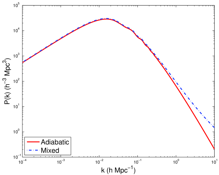
We have given constraints on these parameters with latest observations in Ref. Li:2010yb . The the best fit values are listed in Table 1. Using CAMBcamb , We also sketch the power spectra in Fig. 1 with best fit values.

Table 1: The best fit value for models with different initial conditions.

Parameters	Aidabatic	Mixed
$\Omega_{b}$	$0.046$	$0.044$
$\Omega_{m}$	$0.280$	$0.267$
$\Omega_{\Lambda}$	$0.720$	$0.733$
$h$	$0.700$	$0.714$
$10^{9}A_{s}^{adi}$	$2.176$	$2.420$
$n_{s}^{adi}$	$0.960$	$0.965$
$10^{10}A_{s}^{iso}$	$-$	$0.081$
$n_{s}^{iso}$	$-$	$2.716$
$\cos\Delta$	$-$	$0.173$
$\sigma_{8}$	$0.820$	$0.865$

Figure 1: Linear matter power spectra for the models in Table 1. The red solid line corresponds to standard ${\Lambda}CDM$ model with adiabatic initial condition while the blue dash-dotted line is given by mixed initial condition.

III N-body Simulation

We perform our simulations with GADGET-2gadget , a massively parallel TreePM-SPH (Tree Particle Mesh-Smoothed Particle Hydrodynamics) code. For collisionless particles, the gravitational field is calculated with a low-resolution particle-mesh(PM) algorithm on large scales, while forces are delivered by tree on small scales. We do not use the SPH part since only cold dark matter particles are considered in this work.

III.1 Initial Conditions

With power spectrum plotted in Fig. 1, we can generate positions and velocity ICs for particles at cosmic time $\tau$ using the Zel’dovich Approximations(ZA).

$${\bf x}({\bf q},\tau) = {\bf q}+D^{+}(\tau){\bf\Psi}({\bf q}),$$ (9)

$${\bf v}({\bf q},\tau) = \dot{D}^{+}(\tau){\bf\Psi}({\bf q}),$$ (10)

where ${\bf x}$ is the perturbed comoving coordinates and ${\bf v}\equiv\frac{d{\bf x}}{d{\bf\tau}}$ is the proper peculiar velocity. q, the lagrangian coordinates generated from glass configurationWhite:1994bn , denote the unperturbed comoving position. $D^{+}(\tau)$ is the linear growth factor normalized to $z=0$. ${\bf\Psi}({\bf q})$ is displacement field calculated from the density fluctuation field which is the convolution of a random white noise with the square root of the linear power spectrumSirko:2005uz .

The ICs are set at $z=49$ when the second order Lagrangian perturbations correction can be ignored safely. we run four sets of simulations with different box sizes to explore the differences between two initial conditions on different scales. The larger boxes whose length is $1000~{}\text{h}^{-1}~{}\text{Mpc}$ provide good statistics on large scales from $k\sim 10^{-3}~{}\text{h}~{}\text{Mpc}^{-1}$ to $k\sim 1~{}\text{h}~{}\text{Mpc}^{-1}$, while the smaller boxes with $L=100~{}\text{h}^{-1}~{}\text{Mpc}$ can give high resolution extending to $k\sim 10~{}\text{h}~{}\text{Mpc}^{-1}$. In Set I, the mass resolution is $5.8\times 10^{11}~{}{\text{h}}^{-1}M_{\odot}$ with $N_{p}=512^{3}$ while in Set II the mass resolution is about $2.4\times 10^{9}~{}{\text{h}}^{-1}M_{\odot}$. The force resolution is taken as $\sim 0.5\%$ of the mean particle interval (Tab. LABEL:tab:sim).

Because we can get only one value of $\sigma_{8}$ for a specific survey and to cease the effect of different choices of cosmological parameters, we renormalize the power spectra in Fig. 1 to the same $\sigma_{8}=0.8$. This setting may make results present below not so obvious, however, what we are interested in is the relative difference, which is independent on the renormalization.

Table 2: Simulation details for adiabatic and mixed initial conditions.

	Set I		Set II
Initial Condition	adiabatic	Mixed	adiabatic	Mixed
$L_{box}(h^{-1}Mpc)$	$1000$	$1000$	$100$	$100$
$N_{part}$	$512^{3}$	$512^{3}$	$320^{3}$	$320^{3}$
$L_{soft}(h^{-1}kpc)$	$10$	$10$	$5$	$5$
$z_{start}$	$49$	$49$	$49$	$49$

III.2 Numerical Results

III.2.1 Correlation Function

The baryon acoustic oscillation (BAO), as a standard ruler, is a powerful tool to study the dark energy. It is also a useful tool to detect the dark matter isocurvature perturbation. The presence of dark matter isocurvature perturbation would alter the position of first peak in the CMB angular power spectrum, which is the right scale of BAO. The peak in the two point correlation function and the wiggles in the power spectrum are the useful tools to track the behavior of BAOEisenstein:2005su .

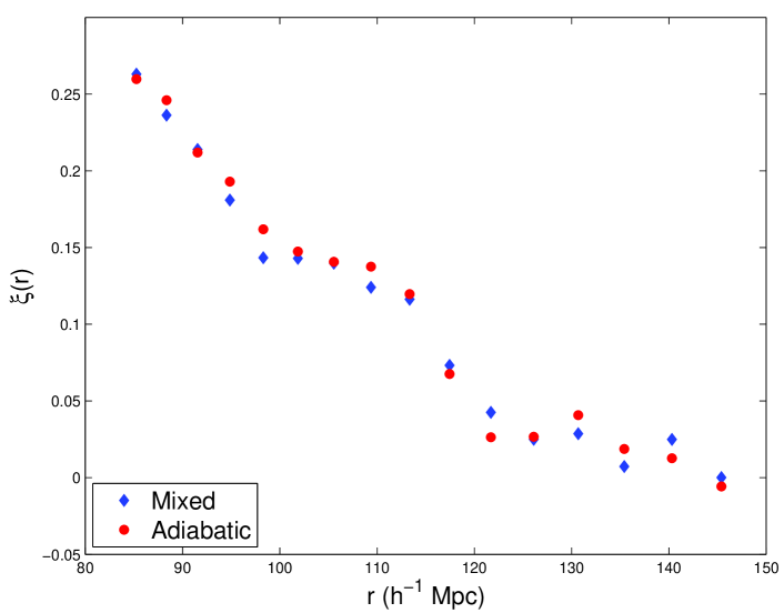
We calculate the 2-point correlation function for Set I at $z=0$ with the pair-count estimator proposed by Landy $\&$ SzalayLandy:1993yu :

$$\xi(r)=\frac{DD-2DR+RR}{RR},$$ (11)

where $DD$ and $RR$ are the autocorrelation function of the simulation particles and randomly sampled points respectively, $DR$ is the cross-correlation between the data and random points. From Fig. 2, we can find that, the position and width of BAO from which $H(z)$ and $D_{A}(Z)$ are extracted, are almost the same for the two different simulations. This result is reasonable in two aspects. Firstly, the BAO observation mainly depends on the background parameter, while has little to do with the origin of the perturbations; secondly, we set ICs with best fit parameters. The behavior on large scales ($k<0.2~{}\text{h}~{}\text{Mpc}^{-1}$) is well constrainedsdssdr7 , especially the position of first peak in the CMB angular power spectrumwmap7 . It implies that, if the isocurvature fraction is small enough, we can not discriminate two initial conditions from BAO observation. This is an important systematic error in constraining dark energy from BAO dataMangilli:2010ut ; Zunckel:2010mm .

Figure 2: The 2-point correlation function for two simulations in the large box at $z=0$. The blue stars denote mixed case while the red points are for adiabatic IC.

III.2.2 Power Spectra

Power spectrum, defined as the Fourier transformation of two point correlation function, is the key physical quantity in understanding clustering properties. With a Gaussian initial condition as selected in this paper, power spectrum gives a complete statistical description of fluctuations.

‘POWMES’ is a power spectrum estimator based on the Taylor expansion of the trigonometric functionsColombi:2008dw . The further ‘foldings’ scheme makes it possible to give an accuracy measurement of power spectrum up to a scale

$$k_{max}=k_{ny}\times 2^{n_{fold}-1},$$ (12)

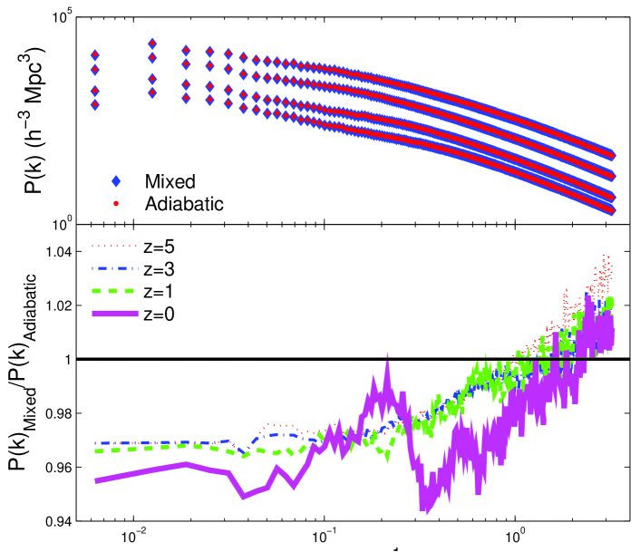
where $k_{ny}=\frac{2\pi}{L_{box}}\frac{N_{p}}{2}$ is the Nyquist frequency and $n_{fold}$ is the number of foldings which is set as $2$ in this work. We plot the power spectra at different redshifts as well as their ratios of Set I in Fig. 3.

Figure 3: Top panel:The power spectrum of simulation Set I. From bottom to top: $z=5$, $z=3$, $z=1$, $z=0$; The blue stars stand for mixed initial condition while red points denote adiabatic $\Lambda$CDM. Bottom panel: the ratio of matter power spectrum between two initial conditions. The thickness is proportional to the scale factor.

From Fig. 3, we can find that power spectra of simulation with mixed IC is smaller than the one in adiabatic case on large scales (small $k$). $r$, the ratio of $P_{mixed}$ to $P_{adiabatic}$, grows as a function of time on large scales, $k>2~{}\text{h}~{}\text{Mpc}^{-1}$ and decreases on small scales, $k<2~{}\text{h}~{}\text{Mpc}^{-1}$. For $k\sim 0.02~{}\text{h}~{}\text{Mpc}^{-1}$, $r$ reaches about $0.95$ at $z=0$. That is to say, the largest discrepancy in power spectrum is about $5\%$.

What we have to keep in mind is that we have renormalized the initial power spectra to the same $\sigma_{8}$ and the weight $k^{2}(\frac{\sin(kr)}{kr^{3}}-\frac{\cos(kr)}{kr^{2}})^{2}$ peaks around $k\sim 0.3~{}\text{h}~{}\text{Mpc}^{-1}$. So, the power spectra we got from N-body simulations with mixed IC should be similar to the one with adiabatic IC on large scales while be larger on small scales without renormalization.

III.2.3 Halo Mass Function

Mass function is defined as the abundance of dark matter haloes in a specific mass ranges. It is a key quantity to describe the large scale structure in the nonlinear regime. Press and Schechter firstly provided the theoretical description in a simple spherical collapse modelPress:1973iz . Subsequently, people made some improvements on this simple modelling and introduced more complex ellipsoidal collapse modelsSheth:1999su . Meanwhile, a lot of literatures try to fit the halo mass function in the manner of N-body simulationSheth:1999mn ; Jenkins:2000bv ; Warren:2005ey ; Tinker:2008ff .

We identify haloes with AHF (Amiga’s Halo Find)AHF , an adaptive mesh based finder. After placing grid across the box and further refinement, AHF assigns each particle to a grid with cloud-in-cell (CIC) interpolation. Then, AHF probes the halo at each density peak using spherical overdensity (SO) algorithm. The radius of sphere is grown until the interior density reaches a specific value

$$\Delta\equiv\frac{M_{\Delta}}{4/3\pi R_{\Delta}^{3}\rho_{bkg}},$$ (13)

where $\rho_{bkg}\equiv\Omega_{m}\rho_{crit}(1+z)^{3}$ is the mean density of whole box. To compare mass functions of these two different models, we set $\Delta$ as $200$ in this paper. With these scheme, AHF can find all structures and substructures simultaneously. Moreover, we only keep haloes with at least 20 dark matter particles, i.e. the mimimum mass of haloes is around $4\times 10^{10}h^{-1}M_{\odot}$.

We introduce the cumulative mass function which is defined as mean number densities of haloes with mass larger than a specific mass,

$$n(>M)=\frac{N(>M)}{L_{box}^{3}},$$ (14)

where $N(>M)$ is the number of haloes with mass greater than M. This is related to the mass function $f(\sigma)$ through

$$n(>m) = \int_{M}^{\infty}\frac{dn}{dM}dM$$ (15)

$$= \int_{M}^{\infty}f(\sigma)\frac{\bar{\rho}_{m}(z=0)}{M}\frac{d\ln\sigma^{-1}}{dM}dM$$

Figure 4: Cumulative mass function as well as the ratio of two situations for simulation Set II. Top left are for $z=3$, top right $z=1$ and bottom left $z=0$. The bottom right is the plot of discrepancy evolvement at $M=5\times 10^{10}M_{\odot}$.

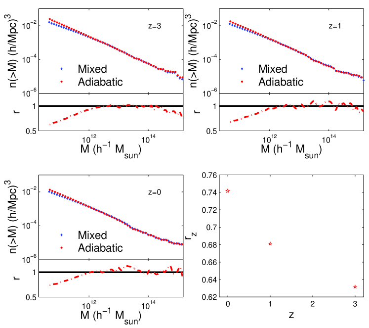
The cumulative mass function as well as the ratio $r\equiv{n_{mixed}}/{n_{adia}}$ for Simulation Set II at redshifts $z=3$, $1$, $0$ are sketched in Fig. 4. We can find that the mass function is almost the same on large mass scale, from $10^{12}M_{\odot}$ to $10^{15}M_{\odot}$. However, there are more haloes for adiabatic IC than for mixed IC on small mass scale ( $M<10^{12}M_{\odot}$ ). Moreover, the discrepancy increases as the mass gets smaller. For $M\sim 5\times 10^{11}M_{\odot}$, the difference is about $26\%$ at $z=0$. We also plot the ratio $r$ against redshift $z$ for $M=5\times 10^{10}h^{-1}M_{\odot}$ in the bottom right of Fig. 4. We find that the ratio decreases as time evolves. Compared to $r=74\%$ at $z=0$, the ratio at $z=3$ is only $63\%$. This behavior can be ascribed to the late-time non-linear evolution. That is to say, a high-redshift survey is helpful to seek the DM isocurvature perturbations signal.

Since we have renormalized to the same $\sigma_{8}$, the power on large scales for mixed IC is less than for adiabatic IC (Fig. 3), and there should be more haloes for mixed IC than for the adiabatic one without renormalization.

IV Summary

Isocurvature perturbations, inevitably generated from multi-field inflation or curvaton models, can be used to test these models. Although pure isocurvature perturbation models have already been ruled out, there still exists possibility that a small fraction of isocurvature mode is correlated to the dominating adiabatic perturbation. This is important to the parameter estimation, since rough ignorance would lead to biased result.

With the best fit values obtained in Ref.Li:2010yb , we perform four sets of N-body simulations to seek a best way to detect the isocurvature perturbations. We find that, if the fraction is small enough($A_{iso}/A_{adia}\sim 3\%$) we can not peek it in the BAO observation. The position and the width of the bump in two-point correlation function, which mainly depend on the background parameter, are almost the same. There are some differences in matter power spectrum and halo mass function. However, the $5\%$ difference in matter power spectra makes it hard to be observed. On the contrary, the deviation in the halo mass function is obvious. The difference is getting larger as we go to higher redshift. For $M\sim 5\times 10^{10}M_{\odot}$ the discrepancy can get $37\%$ at $z=3$. This implies that, with future precise cluster number count observations, we can detect the initial condition of dark matter isocurvature and give stringent constraints.

References

- (1) E. Komatsu et al. [WMAP Collaboration], Astrophys. J. Suppl. 192, 18 (2011).
- (2) B. A. Reid et al., Mon. Not. Roy. Astron. Soc. 404, 60 (2010).
- (3) A. R. Liddle, A. Mazumdar, F. E. Schunck, Phys. Rev. D58, 061301 (1998).
- (4) P. Kanti, K. A. Olive, Phys. Rev. D60, 043502 (1999).
- (5) E. J. Copeland, A. Mazumdar, N. J. Nunes, Phys. Rev. D60, 083506 (1999).
- (6) D. Langlois, Phys. Rev. D59, 123512 (1999).
- (7) D. Wands, N. Bartolo, S. Matarrese and A. Riotto, Phys. Rev. D 66, 043520 (2002).
- (8) Y. S. Piao, R. G. Cai, X. m. Zhang and Y. Z. Zhang, Phys. Rev. D 66, 121301 (2002).
- (9) S. Dimopoulos, S. Kachru, J. McGreevy and J. G. Wacker, JCAP 0808, 003 (2008).
- (10) D. Langlois, S. Renaux-Petel, D. A. Steer and T. Tanaka, Phys. Rev. Lett. 101, 061301 (2008).
- (11) Y. -F. Cai, H. -Y. Xia, Phys. Lett. B677, 226-234 (2009).
- (12) Y. -F. Cai, W. Xue, Phys. Lett. B680, 395-398 (2009).
- (13) Y. -F. Cai, J. B. Dent, D. A. Easson, [arXiv:1011.4074 [hep-th]].
- (14) D. H. Lyth and D. Wands, Phys. Lett. B 524, 5 (2002).
- (15) T. Moroi and T. Takahashi, Phys. Lett. B 522, 215 (2001) [Erratum-ibid. B 539, 303 (2002)].
- (16) D. H. Lyth, C. Ungarelli and D. Wands, Phys. Rev. D 67 (2003) 023503.
- (17) D. Seckel and M. S. Turner, Phys. Rev. D 32, 3178 (1985).
- (18) A. D. Linde, Phys. Lett. B 259, 38 (1991).
- (19) A. D. Linde and V. F. Mukhanov, Phys. Rev. D 56, 535 (1997).
- (20) J. Liu, M. Li and X. Zhang, arXiv:1011.6146 [astro-ph.CO].
- (21) K. Enqvist, H. Kurki-Suonio and J. Valiviita, Phys. Rev. D 62, 103003 (2000).
- (22) C. Gordon, A. Lewis, Phys. Rev. D67, 123513 (2003).
- (23) P. Crotty, J. Garcia-Bellido, J. Lesgourgues et al., Phys. Rev. Lett. 91, 171301 (2003).
- (24) M. Bucher, J. Dunkley, P. G. Ferreira et al., Phys. Rev. Lett. 93, 081301 (2004).
- (25) K. Moodley, M. Bucher, J. Dunkley et al., Phys. Rev. D70, 103520 (2004).
- (26) H. Kurki-Suonio, V. Muhonen, J. Valiviita, Phys. Rev. D71, 063005 (2005).
- (27) M. Beltran, J. Garcia-Bellido, J. Lesgourgues et al., Phys. Rev. D71, 063532 (2005).
- (28) R. Bean, J. Dunkley, E. Pierpaoli, Phys. Rev. D74, 063503 (2006).
- (29) R. Trotta, Mon. Not. Roy. Astron. Soc. 375, L26 (2007).
- (30) I. Sollom, A. Challinor and M. P. Hobson, Phys. Rev. D 79, 123521 (2009).
- (31) J. Valiviita and T. Giannantonio, Phys. Rev. D 80, 123516 (2009).
- (32) M. Beltran, J. Garcia-Bellido, J. Lesgourgues and M. Viel, Phys. Rev. D 72, 103515 (2005).
- (33) A. Mangilli, L. Verde and M. Beltran, JCAP 1010, 009 (2010).
- (34) H. Li, J. Liu, J. Q. Xia and Y. F. Cai, arXiv:1012.2511 [astro-ph.CO].
- (35) C. Zunckel, P. Okouma, S. M. Kasanda, K. Moodley and B. A. Bassett, Phys. Lett. B 696, 433 (2011).
- (36) J. S. Bagla, Curr. Sci. 88, 1088 (2005).
- (37) L. Amendola, C. Gordon, D. Wands and M. Sasaki, Phys. Rev. Lett. 88, 211302 (2002).
- (38) A. Lewis and S. Bridle, Phys. Rev. D 66, 103511 (2002).
- (39) V. Springel, Mon. Not. Roy. Astron. Soc. 364, 1105 (2005).
- (40) S. D. M. White, arXiv:astro-ph/9410043.
- (41) E. Sirko, Astrophys. J. 634, 728 (2005).
- (42) D. J. Eisenstein et al. [SDSS Collaboration], Astrophys. J. 633, 560 (2005).
- (43) S. D. Landy and A. S. Szalay, Astrophys. J. 412, 64 (1993).
- (44) B. A. Reid et al., Mon. Not. Roy. Astron. Soc. 404, 60 (2010).
- (45) S. Colombi, A. H. Jaffe, D. Novikov and C. Pichon, arXiv:0811.0313 [astro-ph].
- (46) S. R. Knollmann and A. Knebe, Astrophys. J. Suppl. 182, 608 (2009).
- (47) W. H. Press and P. Schechter, Astrophys. J. 187 (1974) 425.
- (48) R. K. Sheth, H. J. Mo and G. Tormen, Mon. Not. Roy. Astron. Soc. 323, 1 (2001).
- (49) R. K. Sheth and G. Tormen, Mon. Not. Roy. Astron. Soc. 308, 119 (1999).
- (50) A. Jenkins et al., Mon. Not. Roy. Astron. Soc. 321, 372 (2001).
- (51) M. S. Warren, K. Abazajian, D. E. Holz and L. Teodoro, Astrophys. J. 646, 881 (2006).
- (52) J. L. Tinker et al., Astrophys. J. 688, 709 (2008).