Causal diffusion and its backwards diffusion problem

Abstract

In this article we consider the backwards diffusion problem for a causal diffusion model developed in [25]. Here causality means that the speed of propagation of the concentration is finite. For the investigation of this inverse problem, we derive an analytic representation of the Green function of the causal diffusion model in the $\mathbf{k}-t-$domain (wave vector-time domain). We perform a theoretical and numerical comparison between standard (and noncausal) diffusion with our diffusion model in the $\mathbf{k}-t-$domain and in the $\mathbf{x}-t-$domain. Moreover, we prove that the backwards diffusion problem of the causal diffusion model is ill-posed, but not exponentially ill-posed. In contrast to the classical backwards diffusion problem, the forward operator of the causal direct problem is not compact if the space dimension is $1$. The paper is concluded with numerical simulations of the backwards diffusion problem via the Landweber method.

1 Introduction

The standard model of the backwards diffusion problem is a case example of an exponentially ill-posed problem and it is related to several problems in tomography and image processing. For example, such problems have been studied in the articles [9, 8, 7, 23, 29, 13, 2, 18, 33, 1] and books [21, 10, 24, 22, 34, 26, 28, 14, 30, 31, 31] to name but a few.

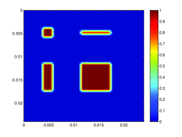
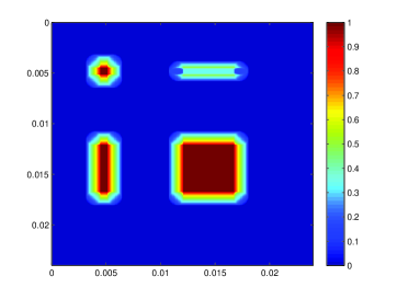
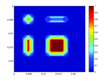
Figure 3: Visualization of causal diffusion for the time sequence $(\frac{\tau}{3},\,\frac{2\,\tau}{3},\,\tau,\,\ldots,\,2\,\tau)$ with discretization $\Delta x=9.6\cdot 10^{-6}$ and $\Delta t=\tau=R/c$. The initial distribution is shown in Fig. 2.

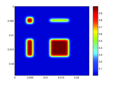
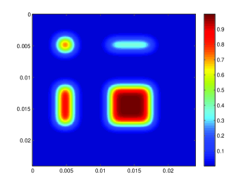
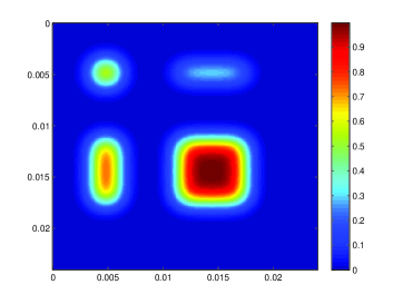
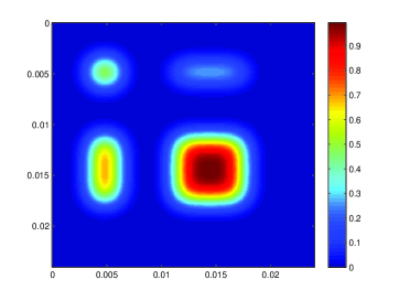
Figure 4: Visualization of standard diffusion for the time sequence $(\frac{\tau}{3},\,\frac{2\,\tau}{3},\,\tau,\,\ldots,\,2\,\tau)$ with discretization $\Delta x:=R/10$ and $\Delta t:=\frac{\Delta x^{2}}{2\,N\,D_{0}}$. The initial distribution is shown in Fig. 2.

This article starts over the backwards diffusion problem by replacing the standard diffusion equation by a causal diffusion model. Recently, such a model has been developed and studied in [25]. By causality we understand that a characteristic feature of a process like an interface or a front must propagate with a finite speed $c$. This means that if a “point concentration” is added to a solution in point $\mathbf{x}={\mathbf{0}}$, then the concentration is zero outside the ball $\overline{B_{c\,T}({\mathbf{0}})}$ after the time period $T$. Here it is not relevant whether this interface or front is visible. Although a causal behavior is naturally demanded for problems involving hyperbolic equations, it is usually disregarded for problems involving parabolic equations. It seem to the author that the modeling of causal equations is quite difficult and unfortunately it is considered as insignificant. Indeed, if a direct problem is smoothing or damping, then after a sufficiently long time period it does not matter if the exact or the perturbed model is used. However, the situation is quite different for the respective inverse and ill-posed problem for which data and modeling errors have a strong impact on the solution. Hence, although our causal diffusion model yields similar numerical values as the standard diffusion model (compare Fig. 3 and Fig. 4), it seems evident that causal diffusion is of practical interest for inverse problems related to diffusion.

Apart from this fact, the modeling and investigation of causal mathematical equations is interesting from the pure mathematical point of view.

The goal of this paper is to investigate to what extent a causal diffusion model influences the respective backwards diffusion problem. We show that this inverse problem is ill-posed, but not exponentially ill-posed. For this purpose we derive basic properties of the causal diffusion model (cf. Section 2 and the appendix) which can be summaries as follows. If $v$ denotes the distribution of a substance diffusing with constant speed $c$ and initial concentration $u$, then we have the following analytic representation

(1) $$\hat{v}(\cdot,m+s)=(2\,\pi)^{-N/2}\,\Upsilon_{N}(|\cdot|)^{m}\,\Upsilon_{N}(|\cdot|\,s)\,\hat{u}$$

for $m\in{\mathbb{N}}_{0}$ and $s\in(0,1]$, where $\hat{v}$ denotes the Fourier transform of $v$ with respect to $\mathbf{x}\in{\mathbb{R}}^{N}$ and $\Upsilon_{N}$ is the solution of

$$\Upsilon_{N}^{\prime\prime}(t)+\frac{(N-1)}{t}\,\Upsilon_{N}^{\prime}(t)+\Upsilon_{N}(t)=0\qquad\quad t>0\,,$$

with initial conditions $\Upsilon_{N}(0+)=1$ and $\Upsilon_{N}^{\prime}(0+)$. For example, for $N=1,\,2,\,3$ we have

(2) $$\Upsilon_{1}(t)=\cos(t),\qquad\Upsilon_{2}(t)=\mbox{J}_{0}(t)\qquad\mbox{and}\qquad\Upsilon_{3}(t)=\mbox{sinc}(t)\,,$$

where $\mbox{J}_{0}$ denotes the Bessel function of first kind and order zero (cf. appendix). We note that from property (1) and $\mbox{supp}(\check{\Upsilon}(\cdot,m+s))=B_{m+s}({\mathbf{0}})$ causality can be infered (cf. (7)). Here $\check{\Upsilon}(\cdot,s)$ denotes the inverse Fourier transform of $\Upsilon(|\cdot|\,s)$. Several important properties of the causal diffusion model are derived from these properties which are in strong contrast to the standard diffusion model (cf. Section 2 and 3).

The respective backwards diffusion problem corresponds to the solution of the Fredholm integral equation of the first kind

$$F_{T}(u)=w\qquad\quad\mbox{for given data $w$,}$$

where the forward operator is defined by $F_{T}(u):=v(\cdot,T)$ with $v$ as in (1) and $T>0$ denotes the data acquisition time. We show (for appropriate spaces) that the forward operator is injective and that it is compact (cf. Section 4)

• if $N=2$ and $T>2\,\tau$ and

• if $N\geq 3$ and $T>\tau$.

Here $N$ denotes the space dimension and $t$ the time. We note that the envelope of the Fourier transform of $F_{T}(u)$ does not decrease exponentially fast. In this sense the inverse problem is not exponentially ill-posed. Furthermore, numerical simulations of the backwards diffusion problem are performed (cf. Section 5), which confirm our theoretical results.

The paper is organized as follows: In Section 2 we present our causal model of diffusion and derive those properties of diffusion that are needed for this paper. For the convenience of the reader we put the technical part that is relevant for Sections 2 and 3 in the appendix. Comparisons between the standard diffusion model and our causal diffusion model are performed in Section 3. The theoretical and numerical aspects of the backwards diffusion problem are investigated in Sections 4 and 5. Numerical simulations of the inverse problem via the Landweber method are presented at the end of Section 5.

2 Causal diffusion and its properties

We now define causal diffusion for the case of a constant speed $c\in(0,\infty)$. For the more general case we refer to [25].

Definition 1.

Let $c,\tau\in(0,\infty)$, ${\rm d}\sigma(\mathbf{x}^{\prime})$ denote the Lebesgue surface measure on ${\mathbb{R}}^{N}$ and $|S_{R}({\mathbf{0}})|$ denote the surface area of the sphere $S_{R}({\mathbf{0}})$. Diffusion with a constant speed $c$ is defined by

(3) $$v_{c,\tau}(\mathbf{x},t)=\int_{S_{R(t)}(\mathbf{x})}\frac{v_{c,\tau}\left(\mathbf{x}^{\prime},\tau_{n(t)}\right)}{|S_{R(t)}({\mathbf{0}})|}\,{\rm d}\sigma(\mathbf{x}^{\prime})\,\quad\mbox{with}\quad v_{c,\tau}|_{t=0}=u\,,$$

where $\tau_{n(t)}:=n(t)\,\tau$ and

$$n(t)\in{\mathbb{N}}_{0}\quad\mbox{such that }\quad t\in(n(t)\,\tau,(n(t)+1)\,\tau]\,,$$

and $R(t):=c\,(t-n(t)\,\tau)$. If $u(\mathbf{x})=\delta(\mathbf{x})$, then we call $G_{c,\tau}:=v_{c,\tau}$ the Green function of diffusion. Here $\delta(\mathbf{x})$ denotes the delta distribution on ${\mathbb{R}}^{N}$.

Let $c>0$, $\tau>0$ and $v_{c,\tau}(\mathbf{x},t)$ be defined as in Definition 1. It follows from induction (cf. Lemma 2 in [25]) that the forward operator

(4) $$F_{T}:L^{1}({\mathbb{R}}^{N})\to L^{1}({\mathbb{R}}^{N}),\,u\mapsto v_{c,\tau}(\mathbf{x},T)\qquad\quad\mbox{($T>0$ fixed)}$$

is well-defined and that $\|u\|_{L^{1}}=\|v_{c,\tau}\|_{L^{1}}$, i.e. causal diffusion satisfies the conservation law of mass. In order to analyse the properties of the forward operator in Section 4, we derive the Fourier representation of the Green function $G_{c,\tau}$ of causal diffusion. In this paper $\hat{f}(\mathbf{k})$ and $\mathcal{F}\{f\}(\mathbf{k})$ denote the Fourier transform of $\mathbf{x}\in{\mathbb{R}}^{N}\mapsto f(\mathbf{x})$. Our definition of the Fourier transform and the respective Convolution Theorem are formulated at the beginning of the Appendix.

Remark 1.

The reader may object that the above definition of causal diffusion is not derived from first principles and that it does not look very similar to standard diffusion. Because of property $\|u\|_{L^{1}}=\|v_{c,\tau}\|_{L^{1}}$, it follows that $v_{c,\tau}$ satisfies a continuity equation and, as shown in the introduction of [25], $v_{c,\tau}$ satisfies approximately Fick’s law. Hence it is reasonable that the causal diffusion model follows from first principles under the side condition of causality. The derivation of our model from microscopic equations is intended to be carried out in the future.

Moreover, because standard diffusion satisfies a strongly continuous semigroup property with respect to time and, as shown in Theorem 2 below, our causal diffusion model satisfies a discrete semigroup property with respect to time, it is evident that both models yield similar numerical results under appropriate conditions (compare Fig. 3 and Fig. 4).

Theorem 1.

Let $G_{c,\tau}$ and $\Upsilon_{N}$ be defined as in Definition 1 and (24) (cf. Appendix), respectively. Then

(5) $$\hat{G}_{c,\tau}(\mathbf{k},s)=\frac{\Upsilon_{N}(|\mathbf{k}|\,c\,s)}{(2\,\pi)^{N/2}}\qquad\mbox{for}\qquad\mathbf{k}\in{\mathbb{R}}^{N},\,s\in(0,\tau]$$

and $\mu_{s}(A):=\int_{A}G_{c,\tau}(\mathbf{x},s)\,{\rm d}\mathbf{x}$ defines a positive measure on the Borel sets. Moreover, (2) and (26) (cf. Appendix) hold.

Proof.

We note that $s\in(0,\tau]$ implies $n(s)=0$ and $R(s)=c\,\tau$. Moreover, we have

$$\int_{S_{R}(\mathbf{x})}f(\mathbf{x}^{\prime})\,{\rm d}\,\sigma(\mathbf{x}^{\prime})\equiv\int_{S_{1}({\mathbf{0}})}f(\mathbf{x}+R\,\mathbf{y})\,R^{N-1}\,{\rm d}\,\sigma(\mathbf{y})\,,$$

$$|S_{R}({\mathbf{0}})|=|S_{1}({\mathbf{0}})|\,R^{N-1}\,.$$

From these facts and Definition 1 with $u(\mathbf{x})=\delta(\mathbf{x})$, it follows that

$$G_{c,\tau}(\mathbf{x},s)=\int_{S_{R(s)}(\mathbf{x})}\frac{\delta(\mathbf{x}^{\prime})}{|S_{R(s)}({\mathbf{0}})|}\,{\rm d}\sigma(\mathbf{x}^{\prime})=\int_{S_{1}({\mathbf{0}})}\frac{\delta(\mathbf{x}+R(s)\,\mathbf{y})}{|S_{1}({\mathbf{0}})|}\,{\rm d}\sigma(\mathbf{y})\,.$$

$\mu_{s}(A)$ is a positive measure, since $G_{c,\tau}(\mathbf{x},s)$ is a positive distribution.

To determine the Fourier transform of $G_{c,\tau}$, we use the following series representation derived in Lemma 2 (cf. Appendix):

$$(2\,\pi)^{N/2}\,\mathcal{F}\left\{\int_{S_{1}({\mathbf{0}})}\frac{\delta(\cdot+c\,s\,\mathbf{y})}{|S_{1}({\mathbf{0}})|}\,{\rm d}\sigma(\mathbf{y})\right\}(\mathbf{k})=\sum_{j=0}^{\infty}(-1)^{j}\cdot a_{2\,j}\cdot(|\mathbf{k}|\,c\,s)^{2\,j}$$

for $s\in(0,\tau]$ with $a_{0}=1$ and

$$a_{2\,j}=\frac{1}{(2\,j)!}\,\frac{1\cdot 3\cdot 5\cdots(2\,j-1)}{N\cdot(N+2)\cdot(N+4)\cdots(N+2\,j-2)}\qquad\mbox{for $j\in{\mathbb{N}}$\,.}$$

In Theorem 9 it is shown that $\Upsilon_{1}(t)=\cos(t)$, $\Upsilon_{2}(t)=\mbox{J}_{0}(|\mathbf{k}|\,c\,s)$ and (26) holds. $\Upsilon_{3}(t)=\mbox{sinc}(t)$ can be concluded from Theorem 9, too, or alternatively from

$$a_{2\,j}=\frac{1}{(2\,j)!}\,\frac{1\,\cdot 3\cdot 5\cdots(2\,j-1)}{3\cdot 5\cdot 7\cdots(2\,j+1)}=\frac{1}{(2\,j+1)!}\,.$$

This concludes the proof. ∎

The following theorem together with Theorem 1 provides us with a complete description of causal diffusion and a mean to compare causal and standard diffusion in the $\mathbf{k}-t-$space (cf. Subsection 3.1).

Theorem 2.

Let $v_{c,\tau}$, $u$ and $G_{c,\tau}$ be defined as in Definition 1. Moreover, let $S_{\tau}$ denote the space convolution operator with kernel $G(\mathbf{x},\tau)$, i.e. $S_{\tau}\,u:=G(\cdot,\tau)*_{\mathbf{x}}u$ for every $u\in L^{1}({\mathbb{R}}^{n})$. Then we have

$$v_{c,\tau}(\cdot,t)=S_{\tau}^{m}\,S_{s}\,u\qquad\mbox{for}\qquad t=\tau_{m}+s,\,s\in(0,\tau]\,,$$

which is equivalent to

(6) $$\hat{v}_{c,\tau}(\cdot,t)=(2\,\pi)^{-N/2}\,\Upsilon_{N}(|\cdot|\,c\,\tau)^{m}\,\Upsilon_{N}(|\cdot|\,c\,s)\,\hat{u}\,.$$

Proof.

The claim follows by induction. Let $m=0$. Then $t=s\in(0,\tau]$ and from Theorem 1, we get

$$(G_{c,\tau}(\cdot,s)*_{\mathbf{x}}u)(\mathbf{x}) =\int_{{\mathbb{R}}^{N}}\int_{S_{1}({\mathbf{0}})}\frac{\delta(\mathbf{x}^{\prime}+c\,s\,\mathbf{y})}{|S_{1}({\mathbf{0}})|}\,u(\mathbf{x}-\mathbf{x}^{\prime})\,{\rm d}\mathbf{x}^{\prime}\,{\rm d}\sigma(\mathbf{y})$$

$$=\int_{S_{1}({\mathbf{0}})}\frac{u(\mathbf{x}+c\,s\,\mathbf{y})}{|S_{1}({\mathbf{0}})|}\,{\rm d}\sigma(\mathbf{y})=v(\mathbf{x},t)\,.$$

Now we assume the induction assumption

$$v(\cdot,r+\tau_{m-1})=S_{\tau}^{m-1}\,S_{r}\,u\qquad\mbox{for}\qquad r\in(0,\tau]\,.$$

Let $t=s+\tau_{m}$ with $s\in(0,\tau]$. From the induction assumption with $r:=\tau$, Theorem 1 and Definition 1, we infer

$$S_{\tau}^{m}\,S_{s}\,u(\mathbf{x})=S_{s}\,S_{\tau}^{m}\,u(\mathbf{x})=S_{s}\,v(\mathbf{x},\tau_{m})$$

$$\qquad=\int_{{\mathbb{R}}^{N}}\int_{S_{1}({\mathbf{0}})}\frac{\delta(\mathbf{x}^{\prime}+c\,s\,\mathbf{y})}{|S_{1}({\mathbf{0}})|}\,v(\mathbf{x}-\mathbf{x}^{\prime},\tau_{m})\,{\rm d}\mathbf{x}^{\prime}\,{\rm d}\sigma(\mathbf{y})$$

$$\qquad=\int_{S_{1}({\mathbf{0}})}\frac{v(\mathbf{x}+c\,s\,\mathbf{y},\tau_{m})}{|S_{1}({\mathbf{0}})|}\,{\rm d}\sigma(\mathbf{y})=v(\mathbf{x},s+\tau_{m})\,,$$

since $n(t)=m$.

Finally, the representation (6) follows from Theorem 1 and the Convolution Theorem (21) (cf. Appendix). This concludes the proof. ∎

Remark 2.

According to Theorem 2 the family of operators $\{S_{\tau_{m}}\,|\,m\in{\mathbb{N}}_{0}\}$ is a discrete semigroup, i.e. $S_{0}$ is the identity and

$$S_{\tau_{m}+\tau_{n}}=S_{\tau_{m}}\,S_{\tau_{n}}\qquad\mbox{for}\qquad m,\,n\in{\mathbb{N}}_{0}\,.$$

Formally, the limit $\tau\to 0$ leads to a continuous semigroup $\{S_{t}\,|\,t\geq 0\}$. Indeed, in Subsection 3.2 we show for the case $N=2$ that the limit $\tau\to 0$ under the side condition $\frac{c^{2}\,\tau}{2\,N}=const.$ yields the standard diffusion model and thus $\lim_{\tau\to 0}\{S_{\tau_{m}}\,|\,m\in{\mathbb{N}}_{0}\}$ is a strongly continuous semigroup on $[0,\infty)$. A consequence of this limit process is that $c\to\infty$, i.e. this limit diffusion process is not causal. Because of these facts, we denote the Green function of standard diffusion by $G_{\infty,0}$.

Corollary 1.

The diffusion model defined by Definition 1 satisfies causality condition

(7) $$\mbox{supp}(G_{c,\tau})\subseteq\{(\mathbf{x},t)\in{\mathbb{R}}^{N}\times[0,\infty)\,|\,|\mathbf{x}|\leq c\,t\}\,.$$

Proof.

We recall that the space convolution of two distributions with compact support $A$ and $B$ is well-defined and its support lies in $A+B:=\cup_{\mathbf{x}\in A}\{\mathbf{x}\}+B$. Moreover, we note that

$$B_{R_{1}}({\mathbf{0}})+B_{R_{2}}({\mathbf{0}})=B_{R_{1}+R_{2}}({\mathbf{0}})\,,$$

where $B_{R}({\mathbf{0}})$ denotes the open ball of radius $R$ and center ${\mathbf{0}}$.

Let $t=s+\tau_{m}$ with $m\in{\mathbb{N}}_{0}$ and $s\in(0,\tau]$. From Definition 1, it follows that $\mbox{supp}(G_{c,\tau}(\mathbf{x},r))\subseteq B_{c\,r}({\mathbf{0}})$ for $r\in(0,\tau]$ and thus by Theorem 2 the support of $G_{c,\tau}(\mathbf{x},t)$ lies in $B_{c\,s+c\,m\,\tau}({\mathbf{0}})=B_{c\,t}({\mathbf{0}})$, which proves the claim. ∎

The following corollary provides us with an alternative definition of causal diffusion and it can be used to compare causal and standard diffusion in the $\mathbf{x}-t-$space (cf. Subsection 3.2).

Corollary 2.

Let $\tau_{m}$ for $m\in{\mathbb{N}}_{0}$ and $v_{c,\tau}$ be defined as in Definition 1 with $u\in L^{1}({\mathbb{R}}^{N})$. The function

$$v(\cdot,s):=v_{c,\tau}(\cdot,\tau_{m}+s)\qquad\mbox{for}\qquad s\in(0,\tau]$$

solves the wave equation

(8) $$\frac{\partial^{2}v}{\partial s^{2}}+\frac{(N-1)}{s}\,\frac{\partial v}{\partial s}-c^{2}\,\nabla^{2}v=0\qquad\mbox{on}\qquad(0,\tau]$$

with initial conditions

(9) $$v(\cdot,0)=v_{c,\tau}(\cdot,\tau_{m})\,\qquad\mbox{and}\qquad\frac{\partial v}{\partial s}(\cdot,0+)=0\,.$$

Here $v_{c,\tau}(\cdot,0)$ ($m=0$) is understood as the initial distribution $u\in L^{1}({\mathbb{R}}^{N})$.

Proof.

From Corollary 5 (cf. Appendix), it follows that

$$\frac{\partial^{2}\Upsilon(|\mathbf{k}|\,c\,s)}{\partial(|\mathbf{k}|\,c\,s)^{2}}+\frac{(N-1)}{|\mathbf{k}|\,c\,s}\,\frac{\partial\Upsilon(|\mathbf{k}|\,c\,s)}{\partial(|\mathbf{k}|\,c\,s)}+c^{2}\,\Upsilon(|\mathbf{k}|\,c\,s)=0\,,$$

where $\mathbf{k}$ and $c$ are fixed. From this, and

$$\hat{v}(\mathbf{k},s)=\Upsilon_{N}(|\mathbf{k}|\,c\,\tau)^{m}\,\Upsilon_{N}(|\mathbf{k}|\,c\,s)\,\hat{u}(\mathbf{k})\,,$$

we obtain

$$\frac{\partial^{2}\hat{v}}{\partial s^{2}}+\frac{(N-1)}{s}\,\frac{\partial\hat{v}}{\partial s}-c^{2}\,{\rm i}^{2}\,|\mathbf{k}|^{2}\,\hat{v}=0\,.$$

But this is equivalent to equation (8). The first initial condition follows from $\Upsilon_{N}(0+)=1$ (cf. Corollary 5) and $\hat{v}_{c,\tau}(\mathbf{k},\tau_{m}+)=\hat{u}(\mathbf{k})\,\Upsilon_{N}(|\mathbf{k}|\,c\,\tau)^{m}$:

$$\hat{v}(\mathbf{k},0+)=\hat{u}(\mathbf{k})\,\Upsilon_{N}(|\mathbf{k}|\,c\,\tau)^{m}\,\Upsilon_{N}(|\mathbf{k}|\,c\,0+)=\hat{v}_{c,\tau}(\mathbf{k},\tau_{m}+)\,.$$

Finally, the second initial condition follows from $\Upsilon^{\prime}(0+)=0$ (cf. Corollary 5):

$$\frac{\partial\hat{v}}{\partial s}(\mathbf{k},0+)=\hat{u}(\mathbf{k})\,\Upsilon_{N}(|\mathbf{k}|\,c\,\tau)^{m}\,\frac{\partial\Upsilon_{N}}{\partial s}(|\mathbf{k}|\,c\,s)|_{s=0+}=0\,.$$

This concludes the proof. ∎

3 Standard diffusion versus causal diffusion

In the following we compare standard and causal diffusion in the $\mathbf{k}-t-$space and the $\mathbf{x}-t-$space. As explained in Remark 2, we denote the Green function of standard diffusion by $G_{\infty,0}$, since $c=\infty$ and $\tau=0$. Similarly we use the notation

$$v_{\infty,0}:=G_{\infty,0}*_{\mathbf{x}}u\qquad\mbox{for}\qquad u\in L^{1}({\mathbb{R}}^{N})\,.$$

3.1 Comparison in the $\mathbf{k}-t-$space

First we recall the definition of the Green function $G_{\infty,0}$ of standard diffusion and establish the link relation

(10) $$D_{0}=\frac{c^{2}\,\tau}{2\,N}\,$$

between the diffusivity $D_{0}$ of standard diffusion and the parameters $c$ and $\tau$ of causal diffusion. Then we compare the Green function of both processes in the $\mathbf{k}-t-$space.

It is well-known that the Green function of standard diffusion reads as follows (cf. e.g. [17, 12, 34, 11, 25])

$$G_{\infty,0}(\mathbf{x},t):=(4\,\pi\,D_{0}\,t)^{-N/2}\,\exp{\left(-\frac{|\mathbf{x}|^{2}}{4\,D_{0}\,t}\right)}\qquad(\mathbf{x}\in{\mathbb{R}}^{N},\,t>0)$$

and that its Fourier transform with respect to $\mathbf{x}$ is given by

(11) $$\hat{G}_{\infty,0}(\mathbf{k},t)=(2\,\pi)^{-N/2}\,\exp{\left(-D_{0}\,|\mathbf{k}|^{2}\,t\right)}\qquad(\mathbf{k}\in{\mathbb{R}}^{N},\,t>0)\,.$$

For sufficiently small $|\mathbf{k}|$ (and $t=\tau$) we have

$$\hat{G}_{\infty,0}(\mathbf{k},\tau)\approx(2\,\pi)^{-N/2}\,\left(1-D_{0}\,|\mathbf{k}|^{2}\,\tau\right)\,.$$

For causal diffusion we get a similar approximation from Theorem 1 together with Lemma 2 (cf. Appendix), namely

$$\hat{G}_{c,\tau}(\mathbf{k},\tau)\approx(2\,\pi)^{-N/2}\,\left(1-\frac{|\mathbf{k}|^{2}\,c^{2}\,\tau^{2}}{2\,N}\right)\,.$$

Comparison of these first order approximations yields the link relation (10).

Remark 3.

Because of

$$2^{a}=e^{a\,\log 2}\qquad\mbox{for}\qquad a\in{\mathbb{R}}\,,$$

the function

(12) $$G_{\#}(\mathbf{x},t):=(4\,\pi\,D_{0}\,t)^{-N/2}\,2^{\left(-\frac{|\mathbf{x}|^{2}}{4\,D_{0}\,t}\right)}\qquad(\mathbf{x}\in{\mathbb{R}}^{N},\,t>0)\,.$$

satisfies the standard diffusion equation with diffusion constant $D_{\#}:=D_{0}/\log(2)$, i.e.

(13) $$\hat{G}_{\#}(\mathbf{k},t)=(2\,\pi)^{-N/2}\,\exp{\left(-D_{\#}\,|\mathbf{k}|^{2}\,t\right)}\,.$$

We use this (perturbed) diffusion model as a third reference model.

For the rest of this subsection we focus on the case $N=3$ for which we have (cf. Theorems 1 and 2):

(14) $$\hat{G}_{c,\tau}(\mathbf{k},\tau_{m}+s) =(2\,\pi)^{-3/2}\,\mbox{sinc}^{m}(|\mathbf{k}|\,c\,\tau)\,\mbox{sinc}(|\mathbf{k}|\,c\,s)\,\qquad s\in(0,\tau]\,.$$

We see that the function $\mathbf{k}\mapsto\hat{G}_{c,\tau}(\mathbf{k},t)$ ($t>0$) is not $C^{\infty}$, since the necessary condition

$$\exists C>0\,\forall m\in{\mathbb{N}}\,\forall\mathbf{k}\in{\mathbb{R}}^{N}:\quad|\hat{G}_{c,\tau}(\mathbf{k},t)|\leq C\,(1+|\mathbf{k}|)^{-m}$$

does not hold (cf. Paley-Wiener-Schwartz Theorem in [20]). Moreover, it is easy to see from (14) that

• $\mathbf{k}\mapsto\hat{G}_{c,\tau}(\mathbf{k},t)$ has a discrete and infinite set of zeros,

• $\mathbf{k}\mapsto\hat{G}_{c,\tau}(\mathbf{k},t_{1})$ and $\mathbf{k}\mapsto\hat{G}_{c,\tau}(\mathbf{k},t_{2})$ have the same zeros if and only if $(t_{1}-t_{2})/\tau\in{\mathbb{N}}_{0}$,

• some of the zeros move with speed $c$ during the time intervals $(\tau_{m-1},\tau_{m}]$ ($m\in{\mathbb{N}}$) such that at the time instants $t=\tau_{m-1}$ and $t=\tau_{m}$ the same set $Z$ of zeros occur. The set $Z$ is given by $\{\mathbf{k}\in{\mathbb{R}}^{3}\,|\,\hat{G}_{c,\tau}(\mathbf{k},\tau)=0\}$.

This behaviour is in contrast to standard diffusion, since $\mathbf{k}\mapsto\hat{G}_{\infty,0}(\mathbf{k},t)$ is $C^{\infty}$ and has no zeros at all. However, since $G_{c,\tau}(\cdot,t)$ has compact support for each $t>0$, the Paley-Wiener-Schwartz Theorem implies a behaviour of such type for causal diffusion.

Now we perform a numerical comparison.

Example 1.

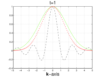
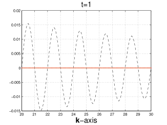
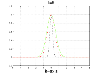
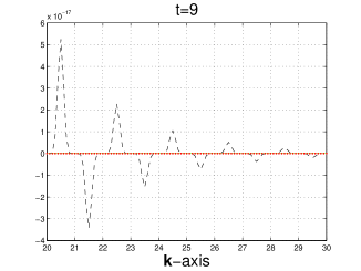
Figure 1: Comparison of $|\mathbf{k}|\mapsto(2\,\pi)^{3/2}\,\hat{G}_{\#}(\mathbf{k},t)$ (dotted red line), $|\mathbf{k}|\mapsto(2\,\pi)^{3/2}\,\hat{G}_{\infty,0}(\mathbf{k},t)$ (solid green line) and $|\mathbf{k}|\mapsto(2\,\pi)^{3/2}\,\hat{G}_{c,\tau}(\mathbf{k},t)$ (dashed black line) . Here $c=1$, $\tau=1$ and $t\in\{\tau,\,9\,\tau\}$.

Let $N=3$, $c=1$, $\tau=1$ and $D_{0}$ be defined as in (10). For these parameters Fig. 1 shows a numerical comparison of the Green function of causal diffusion (14) with the Green functions (11) and (13) of standard diffusion. This and further numerical experiments indicate that

• $\mathbf{k}\mapsto\hat{G}_{\#}(\mathbf{k},t)$ is closer to $\mathbf{k}\mapsto\hat{G}_{\infty,0}(\mathbf{k},t)$ than $\mathbf{k}\mapsto\hat{G}_{c,\tau}(\mathbf{k},t)$,

• if $t$ is large, then $\hat{G}_{\#}(\mathbf{k},t)$, $\hat{G}_{\infty,0}(\mathbf{k},t)$ and $\hat{G}_{c,\tau}(\mathbf{k},t)$ are very small for large $|\mathbf{k}|$,

• $\mathbf{k}\mapsto\hat{G}_{c,\tau}(\mathbf{k},t)$ has a discrete set of zeros, in particular it is not monotone. If $n$ is even, then $\mathbf{k}\mapsto\hat{G}_{c,\tau}(\mathbf{k},t)$ oscillates around zero.

This behavior indicates that modeling errors are a serious issue for the backwards diffusion problem.

3.2 Comparison in the $\mathbf{x}-t-$space

In the following we demonstrate that for an appropiate parameter set a discretization of the standard diffusion equation can yield a similar results as the causal diffusion model introduced in Definition 1.

In order to keep the following formulas and equations short, we focus on the two dimensional case. Consider the diffusion of an image with size of pixel $(\Delta x)^{2}$ and size of time step $\Delta t:=\tau$. We use the notion

$$v_{i,j}^{m}:=v(i\,\Delta x,j\,\Delta x,\tau_{m})\qquad\quad\mbox{for $i,j\in{\mathbb{Z}}$ and $m\in{\mathbb{N}}_{0}$.}$$

If the length of an image pixel $\Delta x$ satisfies (cf. Definition 1)

$$R(\tau)=c\,\tau\equiv\Delta x\,,$$

then we can use the (rough) approximation

$$\int_{|\mathbf{x}-\mathbf{y}|=R(\tau)}\frac{f(\mathbf{x}^{\prime})}{|S_{1}({\mathbf{0}})|}\,d\sigma(\mathbf{y})\approx(f_{i+1,j}+f_{i-1,j}+f_{i,j+1}+f_{i,j-1})/4\,.$$

With this discretization the causal diffusion model (3) is equivalent to

(15) $$\frac{{\color[rgb]{0,0,1}v_{i,j}^{n+1}}-v_{i,j}^{n}}{\tau}=\frac{\Delta x^{2}}{4\,\tau}\,\left[\frac{{\color[rgb]{0,0,1}v_{i+1,j}^{n}}-2\,v_{i,j}^{n}+{\color[rgb]{0,0,1}v_{i-1,j}^{n}}}{\Delta x^{2}}+\frac{{\color[rgb]{0,0,1}v_{i,j+1}^{n}}-2\,v_{i,j}^{n}+{\color[rgb]{0,0,1}v_{i,j-1}^{n}}}{\Delta x^{2}}\right]\,,$$

which is the Forward Euler method of the classical diffusion equation. The classical diffusion equation can be obtained for $\tau\to 0$ under the side condition $\Delta x^{2}/(4\,\tau)=const$, i.e. the diffusivity corresponds to $D_{0}=\Delta x^{2}/(2\,N\,\tau)$ with $N=2$. Carring out this limit process yields $c=\infty$, i.e. the diffusion speed can be interpreted as infinite. In particular, this shows that the discrete semigroup $\{S_{\tau_{m}}\,|\,m\in{\mathbb{N}}_{0}\}$ (cf. Theorem 2) converges to the strongly continuous semigroup of the standard diffusion equation.

Remark 4.

Similarly, the discretization of the wave equation (8) for $N=2$ yields the Forward Euler method of the classical diffusion equation, since

$$\partial_{t}^{2}v+\frac{c}{\tau}\,\partial_{t}v\equiv\frac{v_{i,j}^{n+1}-\not 2\,v_{i,j}^{n}+\not{v_{i,j}^{n-1}}}{\tau^{2}}+\frac{\not v_{i,j}^{n}-\not v_{i,j}^{n-1}}{\tau^{2}}\equiv\frac{\partial_{t}v}{\tau}\,.$$

Here the CFL condition is satisfied for the discretization $\Delta t:=\tau$ and $\Delta x:=c\,\tau$ (cf. [5]). However, to obtain the Forward Euler method we have to neglected the second condition in (9), i.e.

$$\frac{\partial v}{\partial t}(\cdot,\tau_{m}+)=0\qquad\mbox{for all}\qquad m\in{\mathbb{N}}\,.$$

The following numerical example indicates that for sufficiently large time $t$ the forward Euler method (with fine space discretization) can be considered as a noncausal approximation of the causal diffusion model.

Example 2.

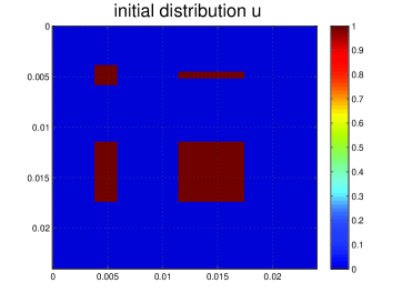
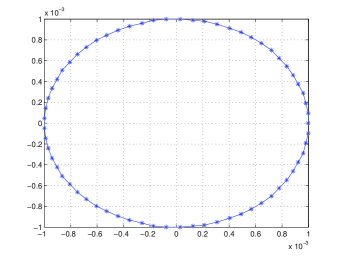
Figure 2: The left picture shows the initial distribution $u$ and the right picture visualizes the discretization of the circle of radius $R=R(\tau)$ that is used to evaluate the circle integrals in Definition 1.

Let N = 2, $c=6.3\cdot 10^{-3}\,m/s$, $R:=10^{-3}\,m$ and $\tau:=R/c$. Here we use the notation $R:=R(\tau)$. To the parameters $c$ and $\tau$ (with $N=2$) of causal diffusion corresponds the diffusion constant $D_{0}:=c^{2}\,\tau/4=1.575\cdot 10^{-6}\,m^{2}/s$ of standard diffusion. The initial mass distribution is shown in Fig. 2. To calculate $v_{c,\tau}$ defined as in Definition 1, the circles with radius $R$ were discretized by $65$ points (cf. Fig. 2). The noncausal distribution $v_{\infty,0}$ was calculated via the forward Euler method for the standard diffusion equation. To guaranteed the convergence of this scheme, the discretization was chosen as $\Delta x:=R/10$ and $\Delta t:=\frac{\Delta x^{2}}{2\,N\,D_{0}}$ such that

$$\frac{\Delta x^{2}}{2\,N\,\Delta t}\geq D_{0}\,$$

holds. A time sequence of $v_{c,\tau}(\cdot,t)$ and $v_{\infty,0}(\cdot,t)$ for the time instants $t=\frac{\tau}{3},\,\frac{2\,\tau}{3},\,\tau,\,\ldots,\,2\,\tau$ is visualized in Fig. 3 and Fig. 4, respectively. As expected each distribution $v_{\infty,0}(\cdot,t)$ is very smooth, in contrast to the distribution $v_{c,\tau}(\cdot,t)$ of causal diffusion. No edge or corner appears in the case of standard diffusion. Although it is not visible, in contrast to $v_{c,\tau}(\cdot,t)$, the support of $v_{\infty,0}(\cdot,t)$ does not lie within the image. For this example, $v_{\infty,0}(\cdot,t)$ and $v_{c,\tau}(\cdot,t)$ are very similar after a time period of about $t=3\,\tau$. Again, we note that this means that modeling errors for the backward diffusion problem is an issue.

4 Basic properties of the forward operator

The calculation of a diffusing substance over the time period $T$ with initial concentration $u\in L^{1}({\mathbb{R}}^{N})$ corresponds to the evaluation of the forward operator (4). We define this as the direct problem and consider the estimation of the initial concentration $u$ from appropriate data $w$. That is to say the solution of the Fredholm integral equation of the first kind

(16) $$F_{T}(u)=w\qquad\quad\mbox{for given data $w$.}$$

This inverse problem requires the knowledge of $c$, $\tau$ and $T$. In this section we investigate the properties of the forward operator and in the subsequent section we discuss and perform numerical simulations of the inverse problem. We use the notation:

Definition 2.

a) Let $T>0$ and $\Omega_{0}$ be an open subset of $B_{r}({\mathbf{0}})$ ($r>0$). Then we define $\Omega_{T}:=B_{r+c\,T}({\mathbf{0}})$. Here $B_{r}({\mathbf{0}})$ denotes the open ball with center ${\mathbf{0}}$ and radius $r$.
b) $L_{c}^{2}({\mathbb{R}}^{N})$ is defined as the space of $L^{2}-$functions with compact support in ${\mathbb{R}}^{N}$.

Theorem 3.

Let $T>0$ and $G_{c,\tau}$ be as in Definition 1. The sets of zeros of $\hat{G}_{c,\tau}(\cdot,T)$ is discrete and countably infinite, and the operator $F_{T}:L_{c}^{1}({\mathbb{R}}^{N})\to L_{c}^{1}({\mathbb{R}}^{N})$ is injective.

Proof.

a) For $t=\tau_{n}+s$ with $n\in{\mathbb{N}}_{0}$ and $s\in(0,\tau]$, we have $\hat{G}_{c,\tau}(\mathbf{k},\tau_{n}+s)=\hat{G}_{c,\tau}(\mathbf{k},\tau)^{n}\,\hat{G}_{c,\tau}(\cdot,s)$. Hence it is sufficient to show that the sets of zeros of $\hat{G}_{c,\tau}(\cdot,s)$ is discrete and countably infinite. Assume that the function $f:\mathbf{k}\mapsto\hat{G}_{c,\tau}(\cdot,s)$ vanishes on a non-empty $M$ with an accumulation point $\mathbf{k}_{0}\in M$. Because $f$ has compact support, it can be extended to an analytic function $f_{ext}:{\mathbb{C}}^{N}\to{\mathbb{C}}^{N}$ such that $f_{ext}(\mathbf{k})=f(\mathbf{k})$ for $\mathbf{k}\in{\mathbb{R}}^{N}$ (Paley-Wiener Theorem). Since $f_{ext}(\mathbf{k})=0$ for $\mathbf{k}\in M$ and $\mathbf{k}_{0}\in M$ is an accumulation point, $f_{ext}$ is the zero function. Thus $M$ must be discrete. (This fact can also be concluded from Theorem 9.) That the set of zeros of $\hat{G}_{c,\tau}(\cdot,s)$ is countably infinite follows from Theorem 9 and the fact that $\Upsilon_{1}(s)=\cos(s)$ and $\Upsilon_{2}(s)=\mbox{J}_{0}(s)$ have countably infinite zeros.
b) For the injectivity of $F_{T}$. Since $u$ and $G_{c,\tau}(\cdot,T)$ have compact support, $\hat{u}$ and $\hat{G}_{c,\tau}(\cdot,T)$ exist and the Convolution Theorem holds (cf. Theorem 7.1.15 in [20]). Hence

$$\mathcal{F}\{F_{T}(u)\}=\hat{G}_{c,\tau}(\mathbf{k},T)\,\hat{u}\,$$

which implies that

$$F_{T}(u)=0\qquad\Rightarrow\qquad u=0$$

is equivalent to

$$\hat{G}_{c,\tau}(\cdot,T)\,\hat{u}=0\qquad\Rightarrow\qquad\hat{u}=0\,.$$

From $\hat{G}_{c,\tau}(\cdot,T)\,\hat{u}=0$ and part a) of the proof we infer that $\hat{u}$ vanishes on a non-empty open set $M$. Because $u$ has compact support, the Paley-Wiener Theorem implies that $\hat{u}$ can be extended to an analytic function $\hat{u}_{ext}$ on ${\mathbb{C}}^{N}$ satisfying $\hat{u}_{ext}(\mathbf{k})=0$ for $\mathbf{k}\in M$. Therefore $\hat{u}_{ext}$ is the zero function and consequently $u$ vanishes. This proves that $F_{T}$ is injective. ∎

Theorem 4.

The operator $F_{T}:L_{c}^{2}({\mathbb{R}}^{N})\to L_{c}^{2}({\mathbb{R}}^{N})$ is positive, linear and self-adjoint.

Proof.

First we show that $F_{T}:L_{c}^{2}({\mathbb{R}}^{N})\to L_{c}^{2}({\mathbb{R}}^{N})$ is well-defined. Because $L_{c}^{2}({\mathbb{R}}^{N})$ is a subspace of a Hilbert space, it is a Hilbert space, too. If $u\in L_{c}^{2}({\mathbb{R}}^{N})$, then $u\in L_{c}^{1}({\mathbb{R}}^{N})$ and thus $F_{T}(u)\in L^{1}({\mathbb{R}}^{N})$. Since $G_{c,\tau}$ and $u$ have compact support, their convolution exist and it has compact support (cf. Theorem 7.1.15 in [20]). Hence we obtain $F_{T}(L_{c}^{2}({\mathbb{R}}^{N}))\subseteq L_{c}^{1}({\mathbb{R}}^{N})$. According to Parseval’s formula and

$$|(2\,\pi)^{N/2}\,\hat{G}(\mathbf{k},t)|\leq C\qquad\mbox{for some constant $C$}\,,$$

which follows from Theorem 9 (cf. Appendix) and Theorem 1, we have

$$\|F_{T}(u)\|_{L^{2}}^{2} =(2\,\pi)^{N}\|\mathcal{F}\{F_{T}(u)\}\|_{L^{2}}^{2}=(2\,\pi)^{N}\,C\,\int_{{\mathbb{R}}^{N}}|\hat{G}(\mathbf{k},t)\,\hat{u}(\mathbf{k})|^{2}\,{\rm d}\mathbf{k}$$

$$\leq C\,\|u\|_{L^{2}}^{2}\,<\infty\,,$$

i.e. $F_{T}(u)\in L_{c}^{2}({\mathbb{R}}^{N})$. Hence the operator is well-defined.

The positivity and linearity of the operator $F_{T}$ follows at once from Definition 1 and Theorem 2, respectively.

Since $G_{c,\tau}(\mathbf{x}-\mathbf{x}^{\prime},T)=G_{c,\tau}(\mathbf{x}^{\prime}-\mathbf{x},T)$, it follows that

$$\langle F_{T}(u),w\rangle_{L^{2}}=\int_{{\mathbb{R}}^{N}}\int_{{\mathbb{R}}^{N}}G_{c,\tau}(\mathbf{x}-\mathbf{x}^{\prime},T)\,u(\mathbf{x}^{\prime})\,w(\mathbf{x})\,{\rm d}\,\mathbf{x}^{\prime}\,{\rm d}\,\mathbf{x}=\langle u,F_{T}(w)\rangle_{L^{2}}$$

for $w\in L_{c}^{2}({\mathbb{R}}^{N})$ and thus $F_{T}$ is self-adjoint. This concludes the proof. ∎

Theorem 5.

If $N=1$ and $T>0$, then $G_{c,\tau}(\cdot,T)$ is a discrete and positive measure and the operator $F_{T}:L^{2}(\Omega_{0})\to L^{2}(\Omega_{T})$ is not compact.

Proof.

Without loss of generality we set $c=1$. According to Theorem 1 we have for $s\in(0,\tau]$:

$$G_{c,\tau}(x,s)=\mathcal{F}^{-1}\{\cos(k\,s)\}(x)=\frac{1}{2}\,[\delta(x-s)+\delta(x+s)]\,,$$

which implies that $G_{c,\tau}(x,T)$ is a convolution of positive distributions with singular support. Therefore $G_{c,\tau}(\cdot,T)$ corresponds to a discrete and positive measure. That $F_{T}$ is not compact follows from the fact that

$$F_{T}=(R_{\tau}+L_{\tau})^{m}\,(R_{s}+L_{s})\qquad\mbox{for}\qquad T=\tau_{m}+s\,,$$

where $R_{s},\,L_{s}:L^{2}({\mathbb{R}})\to L^{2}({\mathbb{R}})$ are noncompact operators defined by

$$R_{s}(u):=u(\cdot-s)\qquad\mbox{and}\qquad L_{s}(u):=u(\cdot+s)\,.$$

∎

Theorem 6.

If $N=2$ and $T>2\,\tau$, then $G_{c,\tau}(\cdot,T)\in L_{c}^{2}({\mathbb{R}}^{2})$ and the operator $F_{T}:L^{2}(\Omega_{0})\to L^{2}(\Omega_{T})$ is compact.

Proof.

Without loss of generality we set $c=1$. Let $T=\tau_{m}+s$ with $m\geq 2$ and $s\in(0,\tau]$. From Theorem 1 together with $|\mbox{J}_{0}(r)|\leq 1$ and the asymptotic behaviour (29) of $\mbox{J}_{0}$ (cf. appendix), we get for $N=2$:

$$\|\hat{G}_{c,\tau}(\cdot,T)\|_{L^{2}({\mathbb{R}}^{2})}^{2} =2\,\pi\,\int_{0}^{\infty}\mbox{J}_{0}^{2\,m}(r\,\tau)\,\mbox{J}_{0}^{2}(r\,s)\,r\,{\rm d}\,r$$

$$\leq A+\frac{2^{3}}{\pi\,\tau\,s}\,\int_{M}^{\infty}\frac{1}{r^{2}}\,{\rm d}\,r\,,$$

where

$$A:=2\,\pi\,\int_{0}^{M}\mbox{J}_{0}^{2\,m}(r\,\tau)\,\mbox{J}_{0}^{2}(r\,s)\,r\,{\rm d}\,r<\infty\,$$

and $M>0$. Because of $\int_{M}^{\infty}1/r^{2}\,{\rm d}\,r=1/M$, we arrive at

$$\|\hat{G}_{c,\tau}(\cdot,T)\|_{L^{2}({\mathbb{R}}^{2})}^{2} =A+\frac{2^{3}}{\pi\,\tau\,s}\,\frac{1}{M}<\infty\,,$$

i.e. $\hat{G}_{c,\tau}(\cdot,T)$ lies in $L^{2}({\mathbb{R}}^{2})$. Consequently, $G_{c,\tau}(\cdot,T)$ lies in $L_{c}^{2}({\mathbb{R}}^{2})$. The compactness of the operator $F_{T}$ (for $N=2$ and $T>2\,\tau$) follows from Theorem 8.15 in [3]. ∎

Theorem 7.

If $N\geq 3$ and $T>\tau$, then $G_{c,\tau}(\cdot,T)\in L_{c}^{2}({\mathbb{R}}^{3})$ and the operator $F_{T}:L^{2}(\Omega_{0})\to L^{2}(\Omega_{T})$ is compact.

Proof.

Without loss of generality we set $c=1$. Let $T=\tau_{m}+s$ with $m\in{\mathbb{N}}$ and $s\in(0,\tau]$. From Theorem 1 and the estimation (27) in Theorem 9, it follows for $N\geq 3$:

$$\|\hat{G}_{c,\tau}(\cdot,T)\|_{L^{2}({\mathbb{R}}^{2})}^{2} =|S_{1}({\mathbf{0}})|\,\int_{0}^{\infty}\Upsilon_{N}^{2\,m}(r\,s)\,\Upsilon_{N}^{2}(r\,s)\,r^{N-1}\,{\rm d}\,r$$

$$\leq|S_{1}({\mathbf{0}})|\,\left(A+C_{N}^{2\,(m+1)}\,\int_{M}^{\infty}\frac{r^{N-1}}{(r\,s)^{(m+1)\,(N-1)}}\,{\rm d}\,r\right)\,,$$

where

$$A:=|S_{1}({\mathbf{0}})|\,\int_{0}^{M}\Upsilon_{N}^{2\,m}(r\,s)\,\Upsilon_{N}^{2}(r\,s)\,r^{N-1}{\rm d}\,r<\infty\,$$

and $M>0$ is sufficiently large. Because of $\int_{M}^{\infty}r^{-(N-1)}\,{\rm d}\,r=-\frac{1}{(N-2)}\,M^{-(N-2)}$, we end up with

$$\|\hat{G}_{c,\tau}(\cdot,T)\|_{L^{2}({\mathbb{R}}^{2})}^{2} =|S_{1}({\mathbf{0}})|\,\left(A+\frac{C_{N}^{2\,(m+1)}}{s^{(m+1)\,(N-1)}\,(N-2)\,M^{N-2}}\right)<\infty\,,$$

i.e. $\hat{G}_{c,\tau}(\cdot,T)$ lies in $L^{2}({\mathbb{R}}^{2})$. As a consequence, $G_{c,\tau}(\cdot,T)$ lies in $L_{c}^{2}({\mathbb{R}}^{2})$. The compactness of the operator $F_{T}$ (for $N=2$ and $T>2\,\tau$) follows from Theorem 8.15 in [3]. ∎

From the Paley-Wiener-Schwartz Theorem (cf. [20]), it follows that the Moore-Penrose inverse $F^{\dagger}$ is uniquely defined by

$$F_{T}^{\dagger}:=(F_{\tau}^{\dagger})^{m}\,F_{s}^{\dagger}\qquad\qquad(\mbox{$T=\tau_{m}+s$, $s\in(0,\tau]$})$$

with

(17) $$\mathcal{F}\{F_{s}^{\dagger}(w)\}(\mathbf{k}):=\,\frac{\hat{w}(\mathbf{k})}{\hat{G}(\mathbf{k},s)}\,\chi_{\Omega_{0}(s)}(\mathbf{k})\qquad\mbox{for}\qquad\mathbf{k}\in\Omega_{0}(s)\,.$$

Therefore if the data lies in

$$\mathcal{R}(F_{T}):=\left\{w\in L_{c}^{2}({\mathbb{R}}^{N})\,\left|\,\frac{\hat{w}}{\hat{G}(\cdot,\tau)^{m}\,\hat{G}(\cdot,s)}\in L^{2}({\mathbb{R}}^{N})\right.\right\}\,,$$

then the initial concentration $u$ can be estimated in principle. In contrast to standard diffusion $\hat{G}(\mathbf{k},s)$ has countably infinite and discrete zeros (cf. Theorem 3). Hence it follows:

Corollary 3.

A necessary condition for $w\in\mathcal{R}(F_{T})$ is that $\hat{w}$ has a zero of order $\geq m$ at $k_{*}$ if $\hat{G}_{c,\tau}(\cdot,T)$ has a zero of order $m$ at $k_{*}$.

According to Theorem 9 for $N\in{\mathbb{N}}$ we have

$$\Upsilon_{N}(t)\asymp t^{(N-1)/2}\qquad\mbox{for}\qquad t\to\infty\,$$

and thus the envelope of $\mathbf{k}\mapsto\hat{G}_{c,\tau}(\mathbf{k},T)$ decreases as

$$\mathbf{k}\mapsto a_{T}\,|\mathbf{k}|^{(\lfloor T/\tau\rfloor+1)\,(N-1)/2}\,\qquad\mbox{for}\qquad|\mathbf{k}|\to\infty\,,$$

where

$$a_{T}:=(c\,\tau)^{\lfloor T/\tau\rfloor\,(N-1)/2}\,\left(c\,(T-\lfloor T/\tau\rfloor\,\tau)\right)^{(N-1)/2}\,.$$

Here $\lfloor a\rfloor$ denotes the largest integer $\leq a$ (and $m\equiv\lfloor T/\tau\rfloor$, $s\equiv T-\tau\,\lfloor T/\tau\rfloor$). Hence we get:

Corollary 4.

If $N=2$ and $T>2\,\tau$ or $N\geq 3$ and $T>\tau$, then the inverse problem (16) is ill-posed, but not exponentially ill-posed.

We end this section with a remark about the technique of time reversal.

Remark 5.

For the special case $T\in(0,\tau]$, it follows from Corollary 2 that the inverse problem (16) depends continuously on the data if the additional data $w_{2}:=\frac{\partial F_{T}(u)}{\partial t}(\cdot,T)$ is known. More precisely, the solution can be calculated by

$$\hat{u}(\mathbf{k})=\chi_{A}(\mathbf{k})\,\frac{\hat{w}(\mathbf{k})}{\Upsilon_{N}(|\mathbf{k}|\,c\,T)}+\chi_{B}(\mathbf{k})\,\frac{\hat{w}_{2}(\mathbf{k})}{|\mathbf{k}|\,c\,\Upsilon_{N}^{\prime}(|\mathbf{k}|\,c\,T)}\,,$$

where $\chi_{A}$ is defined as in (20) and $\{A,\,B\}$ is a covering of ${\mathbb{R}}^{N}$ such that $A\cap B=\emptyset$ and $\Upsilon_{N}(|\cdot|\,T)$ and $\Upsilon_{N}^{\prime}(|\cdot|\,T)$ do not vanish on $A$ and $B$, respectively. Here we have used the fact that the zeros of $\Upsilon_{N}$ and $\Upsilon_{N}^{\prime}$ are of order one which follows from Corollary 5 and Theorem 9 in the appendix.

5 Simulation of the inverse problem

5.1 Simulation of data via a particle method

In order to avoid an inverse crime we calculate the synthetic data for the inverse problem by a particle method (cf. [16]). One of the advantages of a particle method (as long as no mass flows over the boundary) is that the total mass is conserved. For simplicity we focus on the $2D-$case and drop the subscripts $c$ and $\tau$ in $G_{c,\tau}$ and $v_{c,\tau}$.

The particle method

The initial distribution $u$ is approximated by an image, i.e. a piecewise constant function with quadratic pixels of length $\Delta x$. At time instant $t=\tau_{n-1}$ ($n\in{\mathbb{N}}$) the mass concentrated in a pixel separates in $M$ parts and each part propagates on a stright line with constant speed $c$ in a randomly chosen direction ${\mathbf{d}}$ during the time period $\tau$. Here the directions are chosen with equal probability out of the set

$$\{A(\varphi)\,{\mathbf{e}}_{1}\,|\,\varphi=0,\,\pi/M,\,\ldots,\,(M-1)\,\pi/M\}\,,$$

where ${\mathbf{e}}_{1}:=(1,0)^{T}$ and $A(\varphi)$ denotes the matrix that rotates the argument about the angle $\varphi$ in positive direction. This kind of data simulation allows that more than one ”particle” go in the same direction such that a special type of noise is included in the simulated data. To each image pixel is then associated the number of all particles that lie within the pixel multiplied by $1/M$.

Noise

In order to avoid an inverse crime we perturbed the length of the radius $R(\tau)=c\,\tau$ by $\pm 0.25\%$ of its original length (uniformly distributed perturbation). In addition, uniformly distributed $L^{2}-$noise with positive mean value were added to the simulated data. As noise level we have chosen $\delta=0.005$ ($0.5\%$).

Convergence of the particle method

In the following we denote by $G[M](\mathbf{x},t)$ the simulated distribution with initial distribution

$$\delta[M](\mathbf{x}):=\left\{\begin{array}[]{ll}1&\mbox{if $\max(|x|,|y|)<\frac{\Delta x}{2}$}\\ 0&\mbox{elsewhere}\end{array}\right.\,.$$

From analysis it is known that

(18) $$\delta[M](\mathbf{x})\stackrel{{\scriptstyle M\to\infty}}{{\longrightarrow}}\delta(\mathbf{x})\quad\mbox{and}\quad G[M](\mathbf{x},t)\stackrel{{\scriptstyle M\to\infty}}{{\longrightarrow}}G(\mathbf{x},t)\quad\mbox{in}\quad\mathcal{D}^{\prime}({\mathbb{R}}^{2})\,.$$

Here $G$ denotes the Green function of causal diffusion (cf. Definition 1) and $\mathcal{D}^{\prime}({\mathbb{R}}^{2})$ denotes the space of distributions on ${\mathbb{R}}^{2}$. We now show that the algorithm described above for an initial distribution $u$ provides us with an approximate solution of $F_{T}(u)$, were $F_{T}$ denotes the forward operator (4).

Theorem 8.

Let $u\in L_{c}^{1}({\mathbb{R}}^{2})$ and $v(\cdot,t):=G(\cdot,t)*_{\mathbf{x}}u$. For

$$v[M](\cdot,t):=G[M](\cdot,t)*_{\mathbf{x}}u\qquad(t>0)\,,$$

it follows that

$$v[M](\cdot,t)\stackrel{{\scriptstyle M\to\infty}}{{\longrightarrow}}v(\cdot,t)\qquad\mbox{in}\qquad L^{1}({\mathbb{R}}^{2})\,.$$

Proof.

Since the space $C_{0}^{\infty}({\mathbb{R}}^{2})$ is dense in $L^{1}({\mathbb{R}}^{2})$, we assume without loss of generality that $u\in C_{0}^{\infty}({\mathbb{R}}^{2})$. We have

$$\|v[M](\cdot,t)-v(\cdot,t)\|_{L^{1}}=\int_{{\mathbb{R}}^{2}}\left|f[M](\mathbf{x})\right|{\rm d}\mathbf{x}$$

with

(19) $$f[M](\mathbf{x})=\int_{{\mathbb{R}}^{2}}[G[M](\mathbf{x}^{\prime},t)-G(\mathbf{x}^{\prime},t)]\,u(\mathbf{x}-\mathbf{x}^{\prime})\,{\rm d}\mathbf{x}^{\prime}\,.$$

The function $f[M]$ is an element of $C_{0}^{\infty}({\mathbb{R}}^{2})$, since $G[M](\cdot,t)-G(\cdot,t)$ has compact support and $u\in C_{0}^{\infty}({\mathbb{R}}^{2})$ (cf. Proposition 32.1.1 in [15]). From  (18) together with $u\in C_{0}^{\infty}({\mathbb{R}}^{2})$, it follows that the right hand side of (19) converges pointwise and uniformly to zero on compact sets. This together with the fact that $f[M]$ has compact support implies

$$\|v[M](\cdot,t)-v(\cdot,t)\|_{L^{1}}\stackrel{{\scriptstyle M\to\infty}}{{\longrightarrow}}0\,.$$

As was to be shown. ∎

5.2 Numerical solution of the backwards diffusion problem

For solving the inverse problem we use the Landweber method (cf. e.g. [10, 24, 22, 28]). Since $F_{T}:L_{c}^{2}({\mathbb{R}}^{N})\to L_{c}^{2}({\mathbb{R}}^{N})$ is a positive, linear and self-adjoint operator (cf. Theorem 4) the Landweber method reads as follows

$$u_{n+1}=P\{u_{n}-\omega\,F_{T}\,[F_{T}(u_{n})-w^{\delta}]\}\,,$$

where $\omega$ denotes the relaxation parameter, $w^{\delta}$ denotes the noisy data and $P$ denotes the orthogonal projection onto

$$\mathcal{R}(P)=\{u\in L^{2}\,|\,u\geq 0\}\,.$$

The use of the projection operator guarantees that the solution is a positive (mass) distribution. As parameter choice rule we use the discrepancy principle, i.e. the iteration is stopped as soon as

$$\|F_{T}(u_{n+1})-w^{\delta}\|_{L^{2}}<\eta\,\delta\qquad\quad(\eta\geq 2)$$

is true. The relaxation parameter was chosen as

$$\omega:=\frac{1}{4}\,\frac{\|F_{T}(u_{n})-w^{\delta}\|_{L^{2}}^{2}}{\|F_{T}\,[F_{T}(u_{n})-w^{\delta}]\|_{L^{2}}^{2}}\,.$$

In order to avoid an inverse crime, the data $w^{\delta}$ is calculated by the particle method ($M=65$) described above and the calculation of the Forward operator $F_{T}$ in each iteration step is performed by integrals over circles. Each circle is discretized by $50$ points.

We now present two simulations of the backwards diffusion problem for $T=\tau$ and $T=3\,\tau$, respectively.

Example 3.

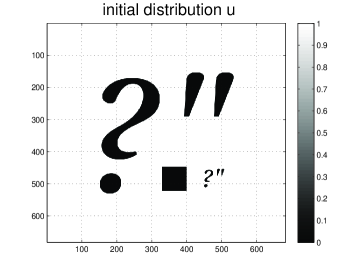
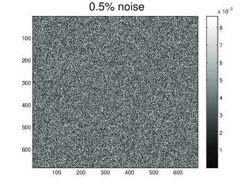
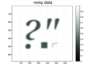
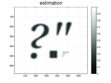
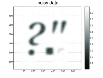
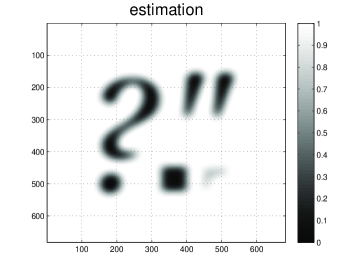
Figure 5: Numerical solution of the inverse problem with $0.5\%$ uniformly distributed $L^{2}$-noise for data acquisition time $T=\tau$ and $T=3\,\tau$. For $T=\tau$ and $T=3\,\tau$, the Discrepancy principle stops optimally for $\eta=9.4$ ($6$ steps) and $\eta=5.9$ ($6$ steps), respectively.

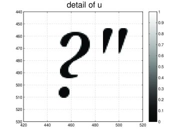
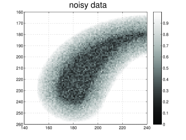
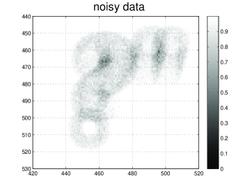
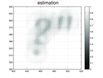
Figure 6: Details to the second row in Fig. 5 ($T=\tau$). The left column shows the left top part of the big question mark and the right column shows the small question mark and the small apostrophe.

Consider the initial distribution shown in Fig. 5. This image consists of $682^{2}$ quadratic pixels of length $\Delta x:=1/681$. As characteristic parameters of causal diffusion we have chosen $c=1$ and $\tau=8\,\Delta x/c$. Hence the characteristic radius $R(\tau)$ is $8$ times $\Delta x$. As described above, the length of the radius $R(\tau)$ was randomly perturbed by $\pm 0.25\%$ of its original length. The data acquisition is performed at time $T=\tau$ and $0.5\%$ (uniformly distributed) $L^{2}-$noise was added to the simulated data. The numerical results are visualized in Fig. 5 and Fig. 6. As expected, the estimation of large structures is much better than for smaller ones. Since the data acquisition is performed at a quite early time the estimation works well. The Discrepancy principle stops optimally for $\eta=9.4$ after $6$ steps.

Example 4.

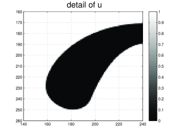
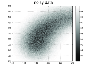
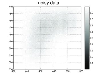
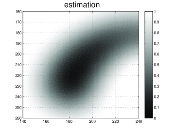
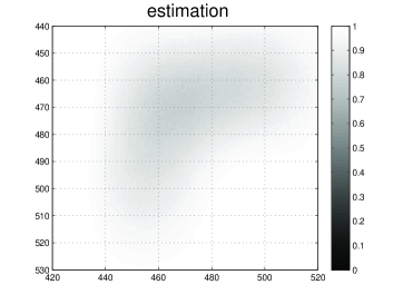
Figure 7: Details to the third row in Fig. 5 ($T=3\,\tau$). The left column shows the left top part of the big question mark and the right column shows the small question mark and the small apostrophe.

We consider the inverse problem from Example 3 again, but for the later data acquisition time $T=3\,\tau$. The Discrepancy principle stops optimally for $\eta=5.9$ after $6$ steps. For this situation the forward operator is compact. As Fig. 7 shows it is not possible to restore the edges of the question mark, since the data are to much “smooth”. This result reflects the ill-posedness of the problem.

6 Appendix

The delta distribution

We use the following notation for the delta distributions. Let $N\in{\mathbb{N}}$ and $\mathbf{x}\in{\mathbb{R}}^{N}$. Then $\delta(\mathbf{x})$ satisfies

$$\int_{{\mathbb{R}}^{N}}f(\mathbf{x})\,\delta(\mathbf{x}-\mathbf{x}_{0})\,{\rm d}\,\mathbf{x}=f(\mathbf{x}_{0})\qquad\mbox{for}\qquad f\in C_{c}({\mathbb{R}}^{N})\,.$$

Here $C_{c}({\mathbb{R}}^{N})$ denotes the set of continuous funtions with compact support. Since $\delta(\mathbf{x})$ has compact support, $C_{c}({\mathbb{R}}^{N})$ can be replaced by $C({\mathbb{R}}^{N})$. In this notation the dirac measure $\mu_{\delta}$ (cf. [27]) reads as follows

$$\mu_{\delta}(A)=\int_{{\mathbb{R}}^{N}}\chi_{A}(\mathbf{x})\delta(\mathbf{x})\,{\rm d}\,\mathbf{x}=\left\{\begin{array}[]{ll}1&\mbox{if ${\mathbf{0}}\in A$}\\ 0&\mbox{elsewhere}\end{array}\right.\,,$$

where

(20) $$\chi_{A}(\mathbf{x}) A\subseteq{\mathbb{R}}^{N}$$ denotes the characteristic function of the set .

In case $N=1$ we use the notation $\delta(x)$ instead of $\delta(\mathbf{x})$.

The Fourier transform

We use the following notation for the Fourier transformation:

$$\hat{f}(\mathbf{k}):=\mathcal{F}\{f\}(\mathbf{k}):=(2\,\pi)^{-N/2}\,\int_{{\mathbb{R}}^{N}}e^{{\rm i}\,\mathbf{k}\cdot\mathbf{x}}f(\mathbf{x})\,{\rm d}\mathbf{x}$$

$$\check{g}(\mathbf{x}):=\mathcal{F}^{-1}\{g\}(\mathbf{x}):=(2\,\pi)^{-N/2}\,\int_{{\mathbb{R}}^{N}}e^{-{\rm i}\,\mathbf{k}\cdot\mathbf{x}}g(\mathbf{k})\,{\rm d}\mathbf{k}\,$$

for $f,\,g\in L^{1}({\mathbb{R}}^{N})$. Here $\mathbf{k}\in{\mathbb{R}}^{N}$ is called the wave vector. In this notation the convolution theorem reads as follows

(21) $$\mathcal{F}\{f_{1}\}\,\mathcal{F}\{f_{2}\}=(2\,\pi)^{-N/2}\,\mathcal{F}\{f_{1}*_{\mathbf{x}}f_{2}\}\qquad f_{1},\,f_{2}\in L^{1}({\mathbb{R}}^{N})\,.$$

Special functions

We define the function $\mbox{sinc}:{\mathbb{R}}\to{\mathbb{R}}$ as the continuous extension of $x\in{\mathbb{R}}\backslash\{0\}\mapsto sin(x)/x$ and recall that the Bessel function of first kind and order zero has the series representation (cf. [19])

(22) $$\mbox{J}_{0}(x)=\sum_{j=0}^{\infty}(-1)^{j}\,\left(\frac{x^{j}}{2^{j}\,j!}\right)^{2}\,.$$

In order to derive an analytic representation of the Fourier transform of the Green function of causal diffusion, we need the following two lemmata.

Lemma 1.

For $N\in{\mathbb{N}}$ with $N>1$ and $j\in{\mathbb{N}}$, let

$$I(N,j):=\int_{-\pi/2}^{\pi/2}\sin^{j}(\varphi)\cos^{N-2}(\varphi)\,{\rm d}\varphi\,.$$

If $j$ is odd, then $I(N,j)=0$ and if $j$ is even, then

(23) $$\frac{I(N,j)}{I(N,0)}=\frac{1\,\cdot 3\cdot 5\cdots(j-1)}{N\cdot(N+2)\cdot(N+4)\cdots(N+j-2)}\,\,.$$

Proof.

If $j$ is odd, then $\sin^{j}(\varphi)\cos^{N-2}(\varphi)$ is an odd function and thus $I(N,j)$ vanishes.

Now let $j$ be even. We perform a proof by induction.

• Let $j=2$. Integration by Parts yields

  $$I(N,2)=\frac{1}{N}\,\int_{-\pi/2}^{\pi/2}\cos^{N-2}(\varphi)\,{\rm d}\varphi=\frac{I(N,0)}{N}\,.$$

• We now assume the induction assumption for $j=m-2$, i.e.

  $$I(N,m-2)=\frac{1\,\cdot 3\cdot 5\cdots(m-3)}{N\cdot(N+2)\cdot(N+4)\cdots(N+m-4)}\,I(N,0)$$

  and prove (23) for $j=m$. Integration by Parts yields

  $$I(N,m)=\frac{m-1}{m+N-2}\,I(N,m-2)\,.$$

  Employing the induction assumption to this result leads to (23) with $j=m$. This concludes the proof.

∎

Lemma 2.

Let

(24) $$\Upsilon_{N}(t):=\sum_{j=0}^{\infty}(-1)^{j}\cdot a_{2\,j}\cdot t^{2\,j}\qquad\mbox{for}\qquad t\in(0,\infty)$$

with $a_{0}=1$ and

$$a_{2\,j}=\frac{1}{(2\,j)!}\,\frac{1\cdot 3\cdot 5\cdots(2\,j-1)}{N\cdot(N+2)\cdot(N+4)\cdots(N+2\,j-2)}\qquad\quad(j\in{\mathbb{N}})\,.$$

The series (24) is absolutely convergent and

$$\int_{S_{1}({\mathbf{0}})}\frac{\delta(\mathbf{x}+c\,s\,\mathbf{y})}{|S_{1}({\mathbf{0}})|}\,{\rm d}\sigma(\mathbf{y})=\frac{\mathcal{F}^{-1}\{\Upsilon_{N}(|\cdot|\,c\,s)\}(\mathbf{x})}{(2\,\pi)^{N/2}}\qquad\mbox{for}\qquad\mathbf{x}\in{\mathbb{R}}^{N},\,s\in(0,\tau]\,.$$

Proof.

That the series representation (24) converges absolutely follows at once from the Quotient Criterion.

Let $\mathbf{x},\,\mathbf{k}\in{\mathbb{R}}^{N}$. From

$$\mathcal{F}\{\delta(\mathbf{x}+a_{1}\,\mathbf{y})\}(\mathbf{k})=(2\,\pi)^{-N/2}\,e^{-{\rm i}\,a_{1}\,(\mathbf{k}\cdot\mathbf{y})}\qquad\quad\mbox{($a_{1}>0$ constant)}$$

and

$$\int_{S_{1}({\mathbf{0}})}e^{a_{2}\,(\mathbf{k}\cdot\mathbf{y})}{\rm d}\sigma(\mathbf{y})=\int_{S_{1}({\mathbf{0}})}e^{a_{2}\,|\mathbf{k}|\,({\mathbf{e}}_{1}\cdot\mathbf{y})}{\rm d}\sigma(\mathbf{y})\qquad\quad\mbox{($a_{2}\in{\mathbb{C}}$ constant)},$$

it follows that

$$\hat{g}(\mathbf{k},s):=\mathcal{F}\left\{\int_{S_{1}({\mathbf{0}})}\frac{\delta(\cdot+c\,s\,\mathbf{y})}{|S_{1}({\mathbf{0}})|}\,{\rm d}\sigma(\mathbf{y})\right\}(\mathbf{k})=\int_{S_{1}({\mathbf{0}})}\frac{e^{-{\rm i}\,({\mathbf{e}}_{1}\cdot\mathbf{y})\,|\mathbf{k}|\,c\,s}}{(2\,\pi)^{N/2}\,|S_{1}({\mathbf{0}})|}\,{\rm d}\sigma(\mathbf{y})$$

for $s\in[0,\tau]$ and $\mathbf{k}\in{\mathbb{R}}^{N}$. Instead of ${\mathbf{e}}_{1}$ we can also use anyone in $\{{\mathbf{e}}_{2},\,{\mathbf{e}}_{3}\,,\ldots,\,{\mathbf{e}}_{N}\}$. Expanding the exponential function yields

(25) $$(2\,\pi)^{N/2}\,\hat{g}(\mathbf{k},s)=\sum_{j=0}^{\infty}(-1)^{j}\,\frac{(|\mathbf{k}|\,c\,s)^{2\,j}}{(2\,j)!}\,d_{2\,j}\,.$$

with

$$d_{j}:=\int_{S_{1}({\mathbf{0}})}\frac{({\mathbf{e}}_{1}\cdot\mathbf{y})^{j}}{|S_{1}({\mathbf{0}})|}\,{\rm d}\sigma(\mathbf{y})\qquad\mbox{for}\qquad j\in{\mathbb{N}}\,.$$

We see at once that $d_{j}=0$ if $j$ is odd and $d_{0}=1$. For the convenience of the reader, we consider the cases $N=1$ and $N>1$ separately.

• For $N=1$ we have ${\mathbf{e}}_{1}\equiv 1$

  $$\int_{S_{1}({\mathbf{0}})}{\rm d}\sigma(\mathbf{y})\equiv\int_{\mathbb{R}}(\delta(y-1)+\delta(y+1))\,{\rm d}\,y\qquad\mbox{and}\qquad|S_{1}({\mathbf{0}})|=2\,,$$

  and thus

  $$d_{j}=\frac{1^{j}+(-1)^{j}}{2}=\left\{\begin{array}[]{ll}1&\mbox{if $j$ is even}\\ 0&\mbox{if $j$ is odd}\end{array}\right.\,.$$

  Inserting this into the series representation yields

  $$(2\,\pi)^{N/2}\,\hat{g}(\mathbf{k},s)=\sum_{j=0}^{\infty}(-1)^{j}\,\frac{(|k|\,c\,s)^{2\,j}}{(2\,j)!}\,.$$

• Let $N>1$. For the derivation of the series representation we use the following $N-$dimensional orthogonal coordinate system (cf. [32])

  $$(r,\varphi_{1},\,\ldots\,,\varphi_{N-1})\in[0,\infty)\times(-\pi,\pi)\times(-\pi/2,\pi/2)^{N-2}$$

  defined by

  $$x_{N}=r\,\sin(\varphi_{N-1})\,,$$

  $$x_{N-1}=r\,\cos(\varphi_{N-1})\,\sin(\varphi_{N-2})\,,$$

  $$x_{N-2}=r\,\cos(\varphi_{N-1})\,\cos(\varphi_{N-2})\,\sin(\varphi_{N-3})\,,$$

  $$x_{N-3}=r\,\cos(\varphi_{N-1})\,\cos(\varphi_{N-2})\,\cos(\varphi_{N-3})\,\sin(\varphi_{N-4})\,,$$

  $$\qquad\qquad\qquad\qquad\vdots$$

  $$x_{2}=r\,\cos(\varphi_{N-1})\,\cdots\,\cos(\varphi_{2})\,\sin(\varphi_{1})\,,$$

  $$x_{1}=r\,\cos(\varphi_{N-1})\,\cdots\,\cos(\varphi_{2})\,\cos(\varphi_{1})\,,$$

  with surface measure

  $${\rm d}\sigma=r^{N-1}\,{\rm d}\varphi_{1}\,\prod_{l=2}^{N-1}\cos^{l-1}(\varphi_{l})\,{\rm d}\varphi_{l}\,.$$

  Since ${\mathbf{e}}_{N}\cdot{\mathbf{e}}_{r}=\sin(\varphi_{N-1})$ and

  $$|S_{1}({\mathbf{0}})|=\int_{S_{1}({\mathbf{0}})}{\rm d}\varphi_{1}\,\prod_{l=2}^{N-1}\cos^{l-1}(\varphi_{l})\,{\rm d}\varphi_{l}\,,$$

  we obtain

  $$d_{j} =\int_{S_{1}({\mathbf{0}})}{\rm d}\varphi_{1}\,\prod_{l=2}^{N-2}\cos^{l-1}(\varphi_{l})\,{\rm d}\varphi_{l}\,\frac{\sin^{j}(\varphi_{N-1})}{|S_{1}({\mathbf{0}})|}\,\cos^{N-2}(\varphi_{N-1})\,{\rm d}\varphi_{N-1}$$

  $$=\frac{I(N,j)}{I(N,0)}$$

  with $I(N,j)$ defined as in Lemma 1. From this and Lemma 1, we obtain $d_{2\,j-1}=0$, $d_{0}=1$ and

  $$d_{2\,j}=\frac{1\,\cdot 3\cdot 5\cdots(2\,j-1)}{N\cdot(N+2)\cdot(N+4)\cdots(N+2\,j-2)}\qquad\mbox{for}\qquad j>0\,.$$

  Inserting this into the series (25) yields the claimed series representation.

This concludes the proof. ∎

The following corollary follows form Lemma 2.

Corollary 5.

For $N\in{\mathbb{N}}$. The function $\Upsilon_{N}$ defined as in (24) satisfies the problem

$$\Upsilon_{N}^{\prime\prime}(t)+\frac{(N-1)}{t}\,\Upsilon_{N}^{\prime}(t)+\Upsilon_{N}(t)=0\qquad\quad t>0\,,$$

with initial conditions

$$\Upsilon_{N}(0+)=1\qquad\mbox{and}\qquad\Upsilon_{N}^{\prime}(0+)=0\,.$$

Here $t=0$ is a regular singular point of the ordinary differential equation.

The following theorem enables us to specify the space Fourier transfrom of the Green function of causal diffusion for every dimension $N$ and to prove some compactness results for the forward operator of causal diffusion.

Theorem 9.

Let $N\in{\mathbb{N}}$ with $N\geq 3$ and $t>0$. The function $\Upsilon_{N}$ defined as in (24) satisfies

(26) $$\Upsilon_{N}(t)=-\frac{(N-2)}{t}\,\Upsilon_{N-2}^{\prime}(t)$$

with

$$\Upsilon_{1}(t)=\cos(t)\qquad\mbox{and}\qquad\Upsilon_{2}(t)=\mbox{J}_{0}(t)\,.$$

Here $\mbox{J}_{0}$ denotes the Bessel function of first kind and order zero. Moreover, we have

(27) $$|\Upsilon_{N}(t)|\leq C_{N}\,t^{-(N-1)/2}\qquad\mbox{for sufficiently large $t$}$$

and some constant $C_{N}>0$.

Proof.

The relation between $\Upsilon_{N}$ and $\Upsilon_{N-2}^{\prime}$ follows at once from the series representation (24). Moreover,

• if $N=1$, then

  $$a_{2\,j}=\frac{1}{(2\,j)!}\,\frac{1\,\cdot 3\cdot 5\cdots(2\,j-1)}{1\cdot 3\cdot 5\cdots(2\,j-1)}=\frac{1}{(2\,j)!}$$

  and thus $\Upsilon(t)=\cos(t)$ and

• if $N=2$, then

  $$a_{2\,j}=\frac{1}{(2\,j)!}\,\frac{1\,\cdot 3\cdot 5\cdots(2\,j-1)}{2\cdot 4\cdot 6\cdots(2\,j)}=\frac{1}{[2\cdot 4\cdot 6\cdots(2\,j)]^{2}}=\frac{1}{[2^{j}\,(j!)]^{2}}\,,$$

  which implies $\Upsilon(t)=\mbox{J}_{0}(t)$ (cf. (22) in the Appendix and [19]).

In order to proof the estimation we use

(28) $$\frac{(t^{N-2}\,\Upsilon_{N}(t))^{\prime}}{(N-2)\,t^{N-3}}=\Upsilon_{N-2}(t)\,,$$

which follows from the series representation (24). We perform a proof by induction. Since $cos(t)$ is bounded and the Bessel function $\mbox{J}_{0}(t)$ satisfies the asymptotic behavior (cf. [4])

(29) $$\mbox{J}_{0}(t)\asymp\sqrt{\frac{2}{\pi\,t}}\,\cos\left(t-\frac{\pi}{4}\right)\qquad\mbox{for}\qquad t\to\infty\,,$$

the estimation holds for $N=1$ and $N=2$. We assume that the estimation (27) holds and prove

$$|\Upsilon_{N+2}(t)|\leq C_{N+2}\,t^{-(N+1)/2}\qquad\mbox{for sufficiently large $t$.}$$

From (26) and (28) we get

$$|\Upsilon_{N+2}(t)| =\left|\frac{N}{t}\,\Upsilon_{N}^{\prime}(t)\right|\leq\frac{N\,(N-2)}{t^{2}}\,(|\Upsilon_{N}(t)|+|\Upsilon_{N-2}(t)|)$$

$$\leq\frac{N\,(N-2)\,(C_{N}+C_{N-2})}{t^{(N+1)/2}}\,,$$

which proves the claim. ∎

References

- [1] M. Addam: An inverse problem for one-dimensional diffusion transport equation in optical tomography. preprint, 2011.
- [2] Y. Ahmadizadeh: Numerical Solution of an Inverse Diffusion Problem Applied Mathematical Sciences, Vol. 1, 2007, no. 18, 863 - 868.
- [3] H. W. Alt: Lineare Funktionalanalysis. Springer Verlag, New York, 4.Auflage, 2000.
- [4] I. N. Bronstein and K. A. Semendjajew: Taschenbuch der Mathematik. Harri Deutsch Verlag, Thun und Frankfurt/Main, 1979.
- [5] R. Courant, K. Friedrichs and H. Lewy: On the partial difference equations of mathematical physics. IBM J. Res. Develop., 11:215–234, 1967.
- [6] R. Dautray and J.-L. Lions: Mathematical Analysis and Numerical Methods for Science and Technology. Volume 5. Springer-Verlag, New York, 1992.
- [7] O. Dorn: A transport-backtransport method for optical tomography. Inverse Problems 14, 1107-1130, 1998.
- [8] A. Elayyan and V. Isakov: On an inverse diffusion problem. SIAM J. Appl. Math., 1997, 57 1737–48.
- [9] H. W. Engl and W. Rundell (eds.): Inverse Problems in Diffusion Processes. SIAM, Philadelphia, 1995.
- [10] H. W. Engl, M. Hanke and A. Neubauer: Regularization of Inverse Problems. Kluwer Academic Publishers, Dordrecht, 1996.
- [11] L. C. Evans: Partial Differential Equations. American Mathematical Society, Providence, Rhode Island, 1999.
- [12] A. L. Fetter and J. D. Walecka: Theoretical Mechanics of Particles and Continua. McGraw-Hill, New York, 1980.
- [13] Y. A. Gryazin, M. V Klibanov and T. R Lucas: Imaging the diffusion coefficient in a parabolic inverse problem in optical tomography. Inverse Problems 15, (1999), 373–397.
- [14] F. Guichard, J.-M. Morel and R. Ryan: Contrast invariant image analysis and PDE’s” Lecture notes, see http://mw.cmla.ens-cachan.fr/ morel/, 2004.
- [15] C. Gasquet and P. Witomski: Fourier Analysis and Applications. Springer Verlag, New York, 1999.
- [16] M. Griebel, S. Knapek, G. Zumbusch and A. Caglar: Numerische Simulation in der Moleküldynamik. Springer-Verlag, New York, 2004.
- [17] C. J. Harris: Mathematical Modelling of Turbulent Diffusion in the Environment. Academic Press, New York, 1979.
- [18] B. M. C. Hetrick, R. Hughes and E. McNabb Regularization of the backwards heat equation via heatlets. Electronic Journal of Differential Equations, Vol. 2008(2008), No. 130, pp. 1–8.
- [19] H. Heuser: Gewöhnliche Differentialgleichungen. Teubner, Stuttgart, 2.Auflage, 1989.
- [20] L. Hörmander: The Analysis of Linear Partial Differential Operators I. Springer Verlag, New York, 2nd edition, 2003.
- [21] V. Isakov: Inverse Source Problems. Math. Surveys and Monographs Series, 34, AMS,Providence, RI, 1990.
- [22] V. Isakov: Inverse Problems for Partial Differential Equations. Springer Verlag, New York, 1998.
- [23] V. Isakov and S. Kindermann: Identification of the coefficient in a one-dimensional parabolic equation. Inverse Problems 16, (2000), 665-680.
- [24] A. Kirsch: An Introduction to the Mathematical Theory of Inverse Problems. Springer Verlag, New York, 1996.
- [25] R. Kowar: On the causality of real-valued semigroups and diffusion. Math. Meth. Appl. Sci. 2012, 35 207-227, (arXiv:1102.3280v1 [math.AP]).
- [26] F. Natterer and F. Wübbeling: Mathematical methods in image reconstruction. Society for Industrial and Applied Mathematics (SIAM), Philadelphia, PA, 2001.
- [27] S. Lang: Real and Functional Analysis Springer-Verlag, New York, 1993.
- [28] A. K. Louis: Inverse und Schlecht gestellte Probleme. Teubner Verlag, Stuttgart 1994.
- [29] V. A. Markel and J. C. Schotland: Inverse problem in optical diffusion tomography. I. Fourier-Laplace inversion formulas. J. Opt. Soc. Am. A. Opt. Image Sci. Vis., 2001, 18(6):1336-47.
- [30] G. Sapiro: Geometric Partial Differential Equations and Image Analysis. Cambridge University Press, Cambridge, 2006.
- [31] O. Scherzer, M. Grasmair, H. Grossauer, M. Haltmeier and F. Lenzen: Variational Methods in Imaging. Springer-Verlag, New York, 2009.
- [32] U. Storch and H. Wiebe: Lehrbuch der Mathematik. Band III. Wissenschaftsverlag, Mannheim, 1993.
- [33] Hui Wei, Wen Chen, Hongguang Sun and Xicheng Li: A coupled method for inverse source problem of spatial fractional anomalous diffusion equations. Inverse Problems in Science and Engineering, 2010, Vol. 18(7), 945–-956.
- [34] J. Weickert: Anistropic Diffusion in Image Processing. Teubner Stuttgart Verlag, Stuttgart, 1998.