TESELA: a new Virtual Observatory tool to determine blank fields for astronomical observations

Abstract

The observation of blank fields, regions of the sky devoid of stars down to a given threshold magnitude, constitutes one of the typical important calibration procedures required for the proper reduction of astronomical data obtained in imaging mode. This work describes a method, based on the use of the Delaunay triangulation on the surface of a sphere, that allows the easy generation of blank fields catalogues. In addition to that, a new tool named TESELA, accessible through the WEB, has been created to facilitate the user to retrieve, and visualise using the VO-tool Aladin, the blank fields available near a given position in the sky.

1 Introduction

Scientific research progress is critically based on the correct exploitation of data obtained at the limit of the technological capabilities. Thus prior to data analysis and interpretation, the quality of the data treatment must be assured in order to guarantee that the information content in that data is preserved. In observational Astrophysics, and in particular imaging with ground-based telescopes, data treatment is performed following data reduction procedures. The main goal of such reduction processes is to minimize the influence of data acquisition imperfections on the estimation of the desired astronomical measurements (see e.g. Gilliland 1992 for a short review on noise sources and reduction processes of CCD data). For this purpose, one must perform appropriate manipulations of data and calibration frames, the latter properly planned and obtained to facilitate the reduction procedure. In this sense, image flatfielding and sky subtraction constitute two of the most common and important reduction steps. Their relevance should not be underestimated, since inadequate flatfielding or sky subtraction easily leads to the introduction of systematic uncertainties in the data. Contrary to random errors, which can be controlled by applying normal statistical methods, the systematic uncertainties can propagate hidden within the arithmetically manipulated data to the final measurements, where their impact may considerably bias their interpretation.

Concerning image flatfielding, the corresponding calibration frames needed to proceed through this reduction step are typically divided into two categories: images intended to provide high-frequency scale sensitivity variations (the pixel-to-pixel response), and images whose goal is to facilitate the removal of the two-dimensional low-frequency scale sensitivity variations of the detectors. The former are usually obtained from continuum lamps (either within the instrument itself or by illuminating a flat screen or the inner dome of the telescope), although the colour of such lamps are not expected to match the spectral energy distributions of the science targets, and ideally dark night sky flats, obtained by pointing the telescope to a blank field should be observed instead. Since this is quite expensive in terms of observing time, this approach is very rarely used. The low-frequency flatfields are usually twilight exposures. The problem here is that the time during which the sky surface brightness is high enough to clearly overpass the signal of any star in the field of view, but not too high to saturate the frames, are placed on two time windows every day, one at the beginning of the evening twilight and the other at the end of the morning twilight. The observational strategy typically consist on obtaining a series of images, shifting the telescope position a few arcseconds between the different exposures in order to avoid the bright stars in the field of view to appear in the same detector pixels. Those pixels are afterwards masked when combining the individual exposures during the reduction procedure. In any case very bright stars need to be avoided since the point spread function of these objects can introduce spikes and artifacts that are not so easily removed during the reduction of the flatfield images. For this purpose the use of blank fields is the best option.

Sky subtraction cannot always be performed by measuring the night sky level in the same frame where the scientific targets are present. This is especially true when the target dimensions are comparable to the detector field of view. In that circumstance separate sky frames are observed, by pointing the telescope to a position devoid of stars as much as possible. For the sky subtraction procedure to be successful, it is essential that these separate sky images are obtained under identical observing conditions, i.e. very close in time and sky position, since this is the only way to prevent varying observing conditions that modify the sky surface brightness.

From the above discussion it is clear that the observation of sky regions devoid of stars down to a given magnitude is a very important aspect to be taken into account when carrying out astronomical observations. To date, no systematic catalogue is available providing the location in the sky of blank fields for varying limiting magnitudes. With modern instrumentation intended to be used in large imaging surveys, the problem is expected to become more demanding. The situation is also starting to be important in spectroscopic observations, since the advent of integral field units with high multiplexing capabilities (and thus, increasingly larger field of view), are expected to be one of the most common instrumentation in ground-based observatories.

The work presented in this paper describes a method that helps to determine the availability of blank fields in any region of the celestial sphere, based on the use of the Delaunay triangulation. The method has been employed to generate catalogues of blank fields to varying limiting magnitudes. In order to facilitate the use of these catalogues, we have created TESELA, a new tool accessible through the WEB which provides a simple interface that allows the user to retrieve the list of blank fields available near a given position in the sky.

Section 2 of this paper describes the method and presents some statistical analysis of its application to the Tycho-2 (Høg et al., 2000) catalogue. Section 3 describes the new tool TESELA. The detailed description of the tessellation of sky subregions is presented in the Appendix.

2 Tessellating the sky

2.1 The Delaunay Triangulation

The Delaunay triangulation (Delaunay, 1934) is a subdivision of a geometric object (e.g. a surface or a volume) into a set of simplices. A simplex, or $n$-simplex to be specific, is the $n$-dimensional analogue of a triangle. More precisely, a simplex is the convex hull (convex envelope) of a set of $(n+1)$ points.

In particular, for the Euclidean planar (2-dimensional) case, given a set of points, also called nodes, the Delaunay triangulation becomes a subdivision of the plane into triangles, whose vertices are nodes. For each of these triangles, it is possible to determine its associated circumcircle, the circle passing exactly through the three vertices of the triangle, and whose center, the circumcentre, can easily be computed as the intersection of the three perpendicular bisectors. Interestingly, in a Delaunay triangulation all the triangles satisfy the empty circumcircle interior property, which states that all the circumcircles are empty, i.e., there are no nodes inside any of the computed circumcircles.

2.2 Applying the Delaunay triangulation to the celestial sphere

Fortunately the Delaunay triangulation is not restricted to the Euclidean 2-dimensional case. It can be applied to other surfaces, in particular to the 2-dimensional surface of a 3-dimensional sphere. In this situation, the tessellation of the spherical surface is built with spherical triangles, i.e., triangles on the sphere whose sides are great circles.

The empty circumcircle interior property of the Delaunay triangulation provides a straightforward method for a systematic search of regions in the celestial sphere free from stars. If one computes the Delaunay triangulation in the 2-dimensional surface of a sphere, using as nodes the location of the stars down to a given threshold visual magnitude ($m$), the above property guarantees that all the circumcircles are void of stars brighter than that magnitude (see Fig. 1). Thus, the circumdiameter of every circumcircle determines the maximum field of view that can be employed in that region of the sky as blank field.

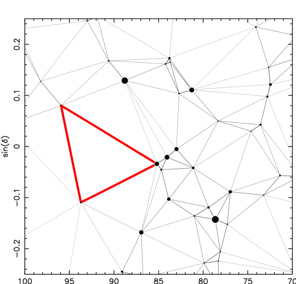
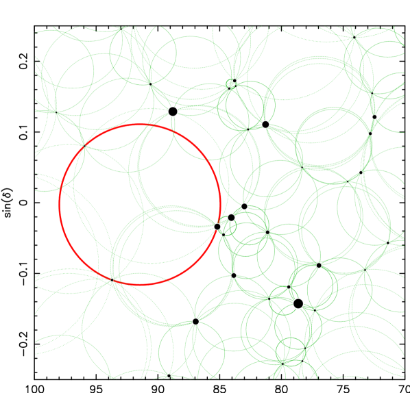
Figure 1: Application of the Delaunay triangulation to the celestial sphere. Left: Sky region centered at the Orion constellation ($\alpha=5^{\mbox{\scriptsize h}}40^{\mbox{\scriptsize m}}$ and $\delta=0^{\circ}$, J2000.0), represented using a Lambert’s equal area projection. All the stars brighter than $m_{V}=4.5$ mag have been considered. Although each star is represented with filled circles of size proportional to its brightness, the triangulation is carried out considering all the stars as nodes for the triangles, independently of their magnitude. A particular triangle is highlighted in red colour. Right:. Circumcircles corresponding to all the triangles derived in the previous triangulation. The red circle indicates the circumcircle associated to the previously highlighted triangle. Note that the empty circumcircle interior property guarantees that there are no stars inside any of the displayed circumcircles.

In this work we have applied the Delaunay triangulation to the Tycho-2 stellar catalogue. Tycho-2 contains astrometric and photometric information for the 2.5 million brightest stars in the sky, and it is complete up to magnitude V = 11.5 mag. Photometric data consists of two pass-bands (B_T and V_T, close to Johnson B and V; Perryman et al. 1997). Typical uncertainties are 60 mas in position and 0.1 mag in photometry. In addition to the main catalogue, we have used the first Tycho-2 supplement, which lists another 17,588 bright stars from the Hipparcos and Tycho-1 Catalogues which are not in Tycho-2.

In order to proceed with the triangulation, we have made use of STRIPACK (Renka, 1997), a Fortran 77 software package that employs an incremental algorithm to build a Delaunay triangulation of a set of points on the surface of the unit sphere. For $N$ nodes, the storage requirement for the triangulation is $13N$ integer storage locations in addition to $3N$ nodal coordinates. The computation scales as $O(N\log N)$. It is important to highlight that the original software was written using single-precision floating arithmetic, which turns out to be insufficient when dealing with astronomical coordinates with accuracy $\sim$ 1 arcsec. For the work presented here, we have modified the software code in order to use double-precision floating arithmetic, which guarantees the proper computation of the triangulation when working with star separations approaching a few arcseconds.

2.2.1 Tessellating a collection of smaller subregions

In principle it is straightforward to obtain a list of blank fields for the whole celestial sphere by using as input a stellar catalogue including stars down to a given magnitude. However, considering that the number of stars grows very rapidly with increasing limiting magnitude, this approach may turn out to become nonviable, either in terms of computer memory or considering computing time. In Fig. 2 we show the time taken by our computer in function of the number of stars (nodes) to carry out the tessellation of the Tycho-2 catalogue. Each dot corresponds to an increase of 0.5 mag in $m_{V_{T}}$, in the range from 6.0 to 10.0 mag. Although the CPU time depends on the characteristic of the machine used for the tessellation, the most important aspect is the exponential increase of the required time with $m_{V_{T}}$, mainly due to the exponential growth of the number of stars (see Table 1). In addition, since the tessellation of the whole celestial sphere demands memory storage (for stellar coordinates plus auxiliary variables) that scales with the number of stars, this approach requires excessively large memory capacity for faint magnitudes.

Figure 2: CPU time consumed in function of the number of stars (nodes) used in the tessellation. Each point corresponds to an increasing $m_{V_{T}}$ from 6 to 10 in steps of 0.5 mag.

In these circumstances our approach is to subdivide the whole celestial sphere in many smaller subregions (with some overlap among them), in order to individually compute the Delaunay triangulation in each of these smaller patches and, finally, merge the separate blank field lists. However the merging process is not immediate, since in this scenario the fact that the triangulation is computed in small subregions have an additional side effect that must be properly handled: when the subregion area is smaller than a single hemisphere, the convex envelope of the stars within that subregion has an interior zone (the subregion) and a larger exterior zone (the celestial sphere excluding the considered subregion). This means that the triangulation has boundary edges, i.e. triangles sides that are not shared with other triangles (see details in Renka, 1997). In practice, the problem arises when one computes the circumcircles of the boundary triangles, since in these cases those circumcircles may easily expand beyond the limits of the considered subregion, where no stars are present because they have not been included as input for the triangulation. A graphical illustration of this problem is shown in Fig. 3.

Figure 3a displays the initial triangulation obtained after computing the Delaunay triangulation of the subregion of the celestial sphere centered around the equatorial coordinates $\alpha=6^{\mbox{\scriptsize h}}$ and $\delta=0^{\circ}$ (J2000.0) within a radius of $30^{\circ}$, and using stars brighter than $m_{V}=4.5$ mag (note that the Orion constellation is close to the center of the field, whereas the bright stars Sirius, Procyon and Aldebaran appear at the South-East, East and North-West, respectively). The sky region is represented using a Lambert’s equal area projection (Calabretta & Greisen, 2002). The thick red line indicates the limit of the $30^{\circ}$ radius. Once the triangulation has been computed, the next step is the calculation of the circumcircle associated to each triangle. Fig. 3b shows all the circumcircles obtained for the triangulation derived in the previous step. The circumcircles that are fully circumscribed within the $30^{\circ}$ radius are displayed with green colour, whereas the circumcircles that expand beyond that limit are represented in magenta. It is obvious that the latter will not be, in general, appropriate blank fields, since they have been computed assuming that no stars were present beyond the red thick line. However, even in these cases several possibilities can be envisaged in order to obtain valid blank fields starting from the information provided by the affected boundary triangles, while respecting the constraint imposed by the proximity of the boundary of the subregion. We discuss in Appendix A several of these possibilities. The result of following such approach is displayed in Fig. 3c.

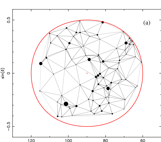
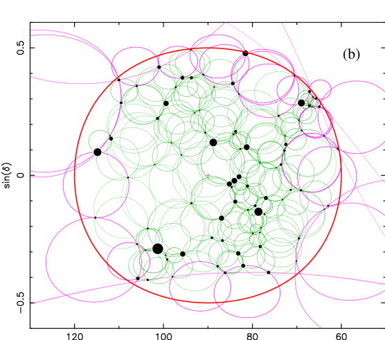
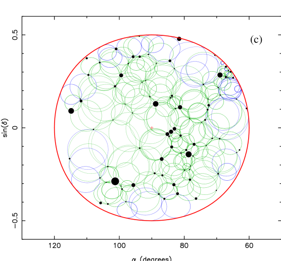
Figure 3: Graphical illustration of the tessellation procedure when handling a subregion of the sky, in particular the portion of the celestial sphere (here represented using a Lambert’s equal area projection) centered around the equatorial coordinates $\alpha=6^{\mbox{\scriptsize h}}$ and $\delta=0^{\circ}$ (J2000.0) within a radius of $30^{\circ}$, and using stars brighter than $m_{V}=4.5$ mag. See explanation in the text (section 2.2.1).

Finally, the blank field lists obtained for the different sky subregions need to be merged. In our case, we have applied this procedure when tessellating the sky for $m_{V_{T}}=10.5$ and 11.0 mag. In particular, we have divided the whole celestial sphere in 578 circular subregions of $8^{\circ}$ radius, where the centre of each subregion is separated by $6^{\circ}$ in declination and by $6^{\circ}/\cos\delta$ in right ascension. Considering that the maximum blank field radius obtained for $m_{V_{T}}=10.0$ mag is $\sim 1^{\circ}$ (see Table 1), this separation between subregions provides an excellent overlap among them. Within the overlapping areas there are duplicated blank fields and additional blank fields that were not permitted to expand beyond their corresponding boundary limit. Consequently, to obtain the final catalogue, we have removed both the repeated blank fields and those due to the border effect (typically inscribed within larger blank fields of neighbouring subregions). The latter were easy to identify because they circumscribe less than 3 stars. Thus, the final all-sky blank field catalogue is not affected by the number, size and overlap of the subregions that we have employed.

2.2.2 Preparing the nodes for the triangulation

As described above, Tycho-2 provides photometry data in two pass-bands (B_T and V_T). We have applied the Delaunay triangulation to each pass-band separately, and to the combination of both. To obtain the initial collections of stars, we have selected from both the main and the supplement Tycho-2 catalogues all stars with magnitude lower than $m$ in a given filter. In the case of using both filters, the star magnitude should be lower than $m$ in either of the two filters.

These initial collections of stars are still not suitable to compute the Delaunay triangulation due to the presence of stars with insufficient separation. For that reason, we decided to “merge” into single objects all the stars closer than 1 arcsec, similar to a typical seeing under good wheather conditions. The resulting visual magnitude for the combined objects was computed as the sum of the fluxes of the merged stars. The coordinates of the new objects were placed in the line connecting the merged stars, closer to the brightest star (using a weighting scheme dependent on the individual brightness of the combined stars). This merging process does not reduce substantially the final number of stars, but it makes the triangulation process easier by removing unnecessary very small triangles for which the computations are prone to rounding errors.

2.3 Results

We have applied the triangulation method to the merged star lists as described above, with threshold magnitudes between 6 and 11 mag in steps of 0.5 mag. The resulting blank field catalogues are accessible through the TESELA tool (explained in section 3).

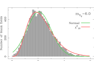
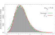
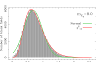
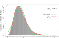
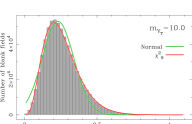
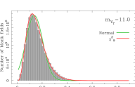
Figure 4: Histograms with the distributions of blank field radius, for different values of $m_{V_{T}}$, as indicated in the upper right inset of each diagram. Note that the x-axis range decreases as $m_{V_{T}}$ increases. The green curve is the fit to a normal distribution, whereas the red line indicates the corresponding fit to a $\chi^{2}_{\nu}$ distribution with $\nu$ degrees of freedom, respectively. The coefficients of these parametric fits are given in Table 1. The best fit in all the diagrams is obtained for the $\chi^{2}_{\nu}$ distribution.

Table 1: Results of the tessellation process using the Tycho-2 catalogue with the V_T filter. Down to $m_{V_{T}}=10$ mag, the Delaunay triangulation has been obtained using the resulting stellar catalogues corresponding to the whole celestial sphere. For $m_{V_{T}}=10.5$ and 11.0, the results correspond to combining the individual triangulation of smaller sky subregions, as explained in the text (see section 2.2.1). The last five rows of this table indicate the coefficients corresponding to the linear regressions $y=a+bx$, where $x=m_{V_{T}}$ in all the cases, and $y$ has been set to the logarithm (with base 10) of the parameters of the remaining columns where the linear fit makes sense. See description of the different columns in Sect. 2.3.

(1)	(2)	(3)	(4)	(5)	(6)	(7)	(8)	(9)	(10)	(11)	(12)	(13)
$m_{V_{T}}$	$N_{*}$	$N_{\mbox{\scriptsize BF}}$	$\rho{\mbox{\scriptsize median}}$	$\Delta h$	$A$	$\overline{\rho}$	$\sigma_{\rho}$	$\rho_{\mbox{\scriptsize max}}$	$B$	$f$	$\nu$	CPU time
(mag)			(deg)	(deg)		(deg)	(deg)	(deg)				(h)
6.0	4,648	9,292	2.111	0.120	$4.796\times 10^{2}$	2.067	0.928	5.805	$4.879\times 10^{2}$	0.436	10	0.02
6.5	8,083	16,162	1.592	0.110	$1.026\times 10^{3}$	1.559	0.691	5.047	$1.033\times 10^{3}$	0.581	11	0.03
7.0	14,229	28,454	1.211	0.080	$1.730\times 10^{3}$	1.182	0.525	3.702	$1.747\times 10^{3}$	0.767	11	0.06
7.5	24,551	49,098	0.914	0.060	$2.938\times 10^{3}$	0.893	0.400	2.932	$2.981\times 10^{3}$	1.011	10	0.15
8.0	41,989	83,974	0.696	0.052	$5.776\times 10^{3}$	0.679	0.302	2.510	$5.830\times 10^{3}$	1.335	11	0.41
8.5	71,491	142,978	0.528	0.042	$1.030\times 10^{4}$	0.514	0.233	2.051	$1.052\times 10^{4}$	1.752	10	1.13
9.0	120,381	240,758	0.405	0.032	$1.707\times 10^{4}$	0.392	0.180	1.557	$1.767\times 10^{4}$	2.294	10	3.21
9.5	200,835	401,666	0.310	0.026	$2.988\times 10^{4}$	0.300	0.140	1.273	$3.128\times 10^{4}$	2.995	10	8.88
10.0	328,819	657,634	0.240	0.022	$5.291\times 10^{4}$	0.231	0.109	1.051	$5.570\times 10^{4}$	3.850	9	23.76
10.5	538,719	1,077,434	0.185	0.020	$1.005\times 10^{5}$	0.177	0.086	0.943	$1.077\times 10^{5}$	4.998	9	—
11.0	871,336	1,742,668	0.143	0.018	$1.850\times 10^{5}$	0.137	0.068	0.853	$2.026\times 10^{5}$	6.460	9	—
$a$	0.96	1.27	1.719	—	$-$0.31	1.725	1.31	1.80	$-$0.35	$-$1.753	—	$-$6.7
$\Delta a$	0.03	0.03	0.011	—	0.04	0.009	0.02	0.05	0.04	0.012	—	0.2
$b$	0.455	0.455	$-$0.2339	—	0.506	$-$0.2362	$-$0.227	$-$0.176	0.513	0.2340	—	0.80
$\Delta b$	0.004	0.004	0.0013	—	0.004	0.0011	0.002	0.006	0.005	0.0014	—	0.03
$r^{2}$	0.9994	0.9994	0.9997	—	0.9992	0.9998	0.9990	0.9901	0.9993	0.9997	—	0.9909

As an example, we present the results of the triangulation for V_T in Fig. 4. The different histograms correspond to the distributions of the number of blank fields as a function of the blank field radius, for different threshold magnitudes $m_{V_{T}}$. The resulting histograms are positively skewed and although, as a first order approach, they can approximately be fitted with a normal distribution (green curves), better fits are obtained using $\chi^{2}_{\nu}$ functions with $\nu$ degrees of freedom (red curves). Note that the use of a chi-square law is just an empirical result, obtained after trying to fit different well-known skewed distributions, like lognormal and $F_{\nu_{1},\nu_{2}}$ distributions (the latter with $\nu_{1}$ and $\nu_{2}$ degrees of freedom), and finding that the best fits were obtained using $F_{\nu_{1},\nu_{2}}$ when $\nu_{2}\rightarrow\infty$, which is equivalent to use a $\chi^{2}_{\nu_{1}}$ distribution (see e.g. Press et al., 2007). It is not the goal of this work to provide a physical justification for this behavior.

The quantitative description of the above results are presented in Table 1. The threshold magnitude $m_{V_{T}}$ is given in the first column. The number of stars $N_{*}$ (i.e. nodes) and the number of blank field regions found $N_{\mbox{\scriptsize BF}}$ are listed in the second and third columns, respectively. The fourth column indicates the median blank field radius $\rho{\mbox{\scriptsize median}}$ and column (5) is the bin width $\Delta h$ for the histogram distributions (some of them displayed in Fig. 4) employed to derive the parametric fits given in the next columns. The amplitude $A$, mean radius $\overline{\rho}$ and standard deviation $\sigma_{\rho}$, obtained from the fit of the each histogram to a normal distribution of the form $A\exp[-(\rho-\overline{\rho})^{2}/(2\sigma^{2}_{\rho})]$ are listed in columns (6) to (8), respectively. The maximum blank field radius appears in column (9). The coefficients of the fit to a chi-square distribution of the form $B\,\chi^{2}_{\nu}(\rho/f)$, where $B$ is the amplitude, $f$ is a scaling factor for $\rho$, and $\nu$ is the number of degrees of freedom, are given in columns (10) to (12). Finally, column (13) indicates the CPU time taken for the triangulation when tessellating the whole celestial sphere at once.

As we have shown in Fig.2, the required CPU computing time increases exponentially with $m$. For this reason, we have derived the Delanuay triangulation for the whole celestial sphere at once just up to magnitude 10, and in overlaping smaller regions (as explained in section 2.2.1) for higher $m$.

2.4 Analysis

We have analysed the results of the triangulation for V_T. For B_T and the combination of both filters the results are very similar.

Not surprisingly, there is an excellent correlation between most of the parameters listed in Table 1 and $m_{V_{T}}$. The correlations can be very well fitted using linear regressions of the form $y=a+bx$, being $x=m_{V_{T}}$ and defining $y$ as the base-10 logarithm of the considered parameter. The intercept $a$ and slope $b$ of the regressions (together with their associated uncertainties $\Delta a$ and $\Delta b$) are given at the bottom of each column. The final entry indicates the coefficient of determination $r^{2}$, which in all the cases reveals the excellent correlation between the fitted data.

It is also interesting to examine the characteristics of the derived blank fields at a given limiting magnitude. For example we have analyzed two illustrative diagrams corresponding to the case $m_{V_{T}}=11.0$, which are represented in Fig. 5. Diagram. 5(a) displays the variation in the number of regions as a function of the absolute value of galactic latitude $l$. Not surprisingly, the number of regions must decrease as the latitude increases, since the area of a spherical annulus (shown with the red symbols) is maximum at the galactic equator and tends to zero when $|l|$ approaches $90^{\circ}$. However, this variation is not enough to explain the difference between the histogram and the red symbols, which clearly indicates that the number of regions is highly concentrated toward the galactic equator, which is simply the result of the higher stellar densitiy in that region. The diagram 5(b) shows that even though the number of available blank fields unavoidably decreases with galactic latitude, their typical size, and the variation of sizes among them, increase with $l$ approaching the galactic poles.

The extrapolation to fainter magnitudes of the exponential variations of the parameters listed in Table 1, together with the unavoidable increasing difficulty when approaching low galactic latitudes, strongly supports the need for an automatic tool that helps to identify suitable blank fields when observing with medium/large size telescopes.

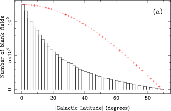
Figure 5: Properties of the blank fields obtained in the case $m_{V_{T}}=11.0$ mag. Diagram (a): number of blank fields as a function of the absolute value of the galactic latitude. The red symbols show the relative variation of the surface area on the celestial sphere with galactic latitude. Diagram (b): variation of the mean circumcircle radius as a function of the absolute value of the galactic latitude (the error bars indicate the root mean square exhibited by the radii at each galactic latitude bin).

3 TESELA

In order to provide an easy way to access the blank field catalogues, we have created TESELA, a WEB accesible tool, developed within the Spanish Virtual Observatory, which can be publicly accessed through the following URL:
http://sdc.cab.inta-csic.es/tesela.

The tool consists of a database containing the Tycho-2 stars and the already computed blank fields regions, and an user-friendly interface for accesing the data. TESELA allows the users to perform a cone-search around a position in the sky, i.e. to obtain the list of blank fields available around a given sky position (right ascension and declination) and within a fixed radius around that position. Through its search form (see Fig.6), users can select the threshold magnitude $m$, the Tycho-2 filter to be used (B_T, V_T, or the combination of both), and define a minimum radius for the blank field regions. This last option may be especially important to fulfill observing requirements, e.g., to ensure that the blank field is larger than the field of view of a given instrument.

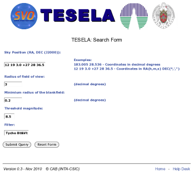
Figure 6: TESELA’s search form. Through it the user defines the value of several parameters used for the cone-search. This form is available at
http://sdc.cab.inta-csic.es/tesela

TESELA presents the result of the cone-search in two tables, one for blank fields (RA, DEC, radius) and the other for the Tycho-2 stars (RA, DEC, $m_{B_{T}}$ and/or $m_{V_{T}}$) in the searching area. These tables can be downloaded in CSV format for further use. TESELA also provides users with the possibility of visualizing the data. To do that, TESELA takes advantage of Aladin Bonnarel et al. (2000), a Virtual Observatory (VO) compliant software that allows users to visualise and analyse digitised astronomical images, and superimpose entries from astronomical catalogues or databases available from the VO services. Thanks to this connection with Aladin, we have provided TESELA with the full capacity and power of the VO.

Figure 7: Example of visualization of the data with Aladin. The large red circle defines the searching area, Tycho-2 stars are shown by red diamonds, the blue circles depict the blank fields, and the black sails are the objects of the NGC 2000.0 in the region.

In Fig. 7 we show an example of how TESELA visualizes the data using Aladin. TESELA sends to Aladin the Tycho-2 stars of the region, which are loaded in the first plane. The search area is plotted in a second layer with a red circle; another layer depicting the blank fields with blue circles is created, and finally, a last layer shows the objects of NGC 2000.0 (The Complete New General Catalogue and Index Catalogue of Nebulae and Star Clusters; Sinnott 1997). Using this Aladin window, users are allowed to load images and catalogues both locally and from the VO, having full access to the whole universe resident in the VO. This can be very helpful to determine the potential influence of relatively bright nebulae and extragalactic sources in the sought regions. Note also that, for obvious reasons, Solar System objects have been not considered, and they must be taken into account in order to make use of blank field regions close to the Ecliptic at a given date.

So far, the current version of TESELA allows users to access a collection of blank fields obtained from the optical Tycho-2 catalogue. But Tesela has been conceived as a dynamic tool, which will be improved in the future with both deeper optical catalogues and catalogues in others wavelength ranges. Any future change in the tool will be properly documented in its web site.

Appendix A Handling boundary triangles

Although tessellating small sky subregions is a good approach to the problem of deriving blank fields when dealing with very large stellar catalogues, the discussion of Section 2.2.1 revealed that the Delaunay triangulation of such subregions leads to the situation displayed in Fig. 3b, where many circumcircles associated to boundary triangles (shown in magenta colour in that figure) clearly expand beyond the limit of the considered subregion. Although in this case those circumcircles can be easily discarded, it is possible to derive, starting from the coordinates of the corresponding boundary triangles, new circles devoided of stars that remain within the boundary of the sky subregion. This appendix describes in more detail different approaches that can be employed in this circumstance.

In what follows we are considering the celestial sphere as the unit sphere centered at the origin $\mn@boldsymbol{O}$. The sky subregion where the blank fields will be searched for is the surface of a spherical cap, which center is given by the unit vector $\mn@boldsymbol{K_{\mbox{\scriptsize sky}}}$, and the angular radius of such subregion, as measured from $\mn@boldsymbol{O}$, is $\theta_{\mbox{\scriptsize max}}$ (see Fig. 8). The Delaunay triangulation will be computed with all the stars (down to a given magnitude) within that sky subregion. Denoting the unit vectors poiting to these stars as $\mn@boldsymbol{S_{i}}$ (with $i=1,\ldots,N_{\mbox{\scriptsize stars}}$, being $N_{\mbox{\scriptsize stars}}$ the total number of stars within the subregion), it is obvious that the condition that all these stars must satisfy is

$$\theta_{\mbox{\scriptsize max}}\geq\mbox{arccos}(\mn@boldsymbol{K_{\mbox{\scriptsize sky}}}\cdot\mn@boldsymbol{S_{i}}),\,\,\forall i=1,\ldots,N_{\mbox{\scriptsize stars}}.$$ (1)

We are also assuming that $\theta_{\mbox{\scriptsize max}}<\pi/2$, i.e., the sky subregion area under consideration is smaller than a single hemisphere.

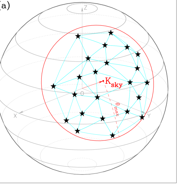
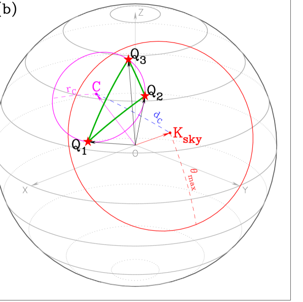
Figure 8: Graphical illustration of the notation employed in Appendix A to explain the initial steps when handling boundary triangles. Diagram (a): The whole celestial sphere of unit radius and centered at the origin $\mn@boldsymbol{O}$ is displayed in gray. The sky subregion under tessellation, which boundary is shown in red, is centered at the point indicated by the unit vector $\mn@boldsymbol{K_{\mbox{\scriptsize sky}}}$, and has a radius $\theta_{\mbox{\scriptsize max}}$ (dashed red line) measured along a great circle on the surface of the celestial sphere. Only the stars contained within this region are employed to compute the Delaunay triangulation (shown in cyan). Diagram (b): A sample boundary triangle formed by the stars located at $\mn@boldsymbol{Q_{1}}$, $\mn@boldsymbol{Q_{2}}$ and $\mn@boldsymbol{Q_{3}}$, given in counterclockwise order, is represented in green. Its corresponding circumcircle, centered at $\mn@boldsymbol{C}$ and passing through the three node stars, is displayed in magenta. The radius of this circumcircle $r_{C}$ is plotted with a dashed magenta line. The angular distance $d_{C}$ between $\mn@boldsymbol{C}$ and $\mn@boldsymbol{K_{\mbox{\scriptsize sky}}}$ is shown with a dashed blue line. In this example the circumcircle expands beyond the limit of the sky subregion, i.e. the condition given in Eq. 4 does not hold.

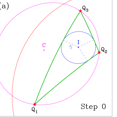
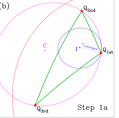
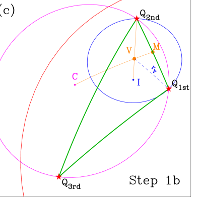
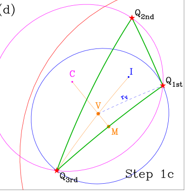
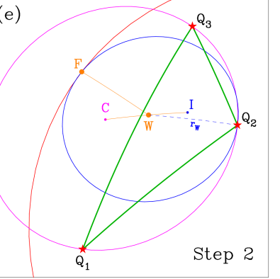
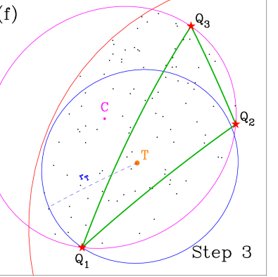
Figure 9: Different strategies described in Appendix A to obtain a valid blank field in the neighborhood of a boundry triangle. These diagrams represent an enlargement of the example represented in Fig. 8, where, for clarity, some graphical elements represented in that figure have been removed.
— Diagram (a): Computation of the incircle, the circle inscribed in the spherical triangle. It is centered at $\mn@boldsymbol{I}$ and is displayed in blue. The distance from $\mn@boldsymbol{I}$ to each of the sides of the boundary triangle is the same, $r_{I}$.
— Diagram (b): Enlargement of the initial incircle until reaching the closest star in the boundary triangle. Note that the three stars at the vertices of the spherical triangle have been renamed as $\mn@boldsymbol{Q_{\mbox{\scriptsize 1st}}}$, $\mn@boldsymbol{Q_{\mbox{\scriptsize 2nd}}}$ and $\mn@boldsymbol{Q_{\mbox{\scriptsize 3rd}}}$ to indicate their order of proximity to the incenter. Thus the resulting new radius, $r_{I,{\mbox{\scriptsize enlarged}}}$, is the angular distance between the incircle $\mn@boldsymbol{I}$ and $\mn@boldsymbol{Q_{\mbox{\scriptsize 1st}}}$.
— Diagram (c): Displacement of the center of the blank field along the great circle connecting the incenter $\mn@boldsymbol{I}$ with the second nearest triangle node $\mn@boldsymbol{Q_{\mbox{\scriptsize 2nd}}}$. The new center $\mn@boldsymbol{V}$ is equidistant to the nodes $\mn@boldsymbol{Q_{\mbox{\scriptsize 1st}}}$ and $\mn@boldsymbol{Q_{\mbox{\scriptsize 2nd}}}$.
— Diagram (d): Displacement of the center of the blank field along the great circle connecting the incenter $\mn@boldsymbol{I}$ with the furthest triangle node $\mn@boldsymbol{Q_{\mbox{\scriptsize 3rd}}}$. The new center $\mn@boldsymbol{V}$ is equidistant to the nodes $\mn@boldsymbol{Q_{\mbox{\scriptsize 1st}}}$ and $\mn@boldsymbol{Q_{\mbox{\scriptsize 3rd}}}$.
— Diagram (e): Displacement of the center of the blank field along the great circle connecting the incenter $\mn@boldsymbol{I}$ and the circumcenter $\mn@boldsymbol{C}$. The distance $r_{W}$ from the new center $\mn@boldsymbol{W}$ to the nearest triangle star is the same than the distance to the boundary of the sky subregion, indicated by $\mn@boldsymbol{F}$.
— Diagram (f): Random search of a valid blank field around the spherical triangle defined by $\mn@boldsymbol{Q_{1}}$, $\mn@boldsymbol{Q_{2}}$ and $\mn@boldsymbol{Q_{3}}$. The black dots are random points in the intersection of the circumcircle and the sky subregion. Each of these points is checked as the center of a potential blank field. The blue circle, with center $\mn@boldsymbol{T}$ and radius $r_{T}$, indicates the largest of such circles that satisfy the conditions for a valid blank field.

Discovering problematic boundary circumcircles

The Delaunay triangulation provides the coordinates of the three nodes (stars) of all the triangles resulting from the tessellation procedure (see Fig. 8). Let denote the unit vectors pointing from $\mn@boldsymbol{O}$ toward the three nodes of each triangle, given in counterclockwise order, as $\mn@boldsymbol{Q_{1}},\mn@boldsymbol{Q_{2}},\mn@boldsymbol{Q_{3}}$, The unit vector $\mn@boldsymbol{C}$ marking the circumcentre of any triangle can be easily computed as (see e.g. Renka, 1997)

$$\mn@boldsymbol{C}=\frac{(\mn@boldsymbol{Q_{2}}-\mn@boldsymbol{Q_{1}})\times(\mn@boldsymbol{Q_{3}}-\mn@boldsymbol{Q_{1}})}{||(\mn@boldsymbol{Q_{2}}-\mn@boldsymbol{Q_{1}})\times(\mn@boldsymbol{Q_{3}}-\mn@boldsymbol{Q_{1}})||}.$$ (2)

Note that since the three nodes define a plane, the two vectors $(\mn@boldsymbol{Q_{2}}-\mn@boldsymbol{Q_{1}})$ and $(\mn@boldsymbol{Q_{3}}-\mn@boldsymbol{Q_{1}})$ are contained in that plane, and their cross product provides a new vector perpendicular to the plane. Of the two possible directions of that vector, the fact that the nodes are given in counterclockwise order guarantees that $\mn@boldsymbol{C}$ points toward the spherical triangle defined by $\mn@boldsymbol{Q_{1}}$, $\mn@boldsymbol{Q_{2}}$, and $\mn@boldsymbol{Q_{3}}$. In addition, the modulus calculated in the denominator of Eq. 2 assures that $\mn@boldsymbol{C}$ is normalised. It is not difficult to show that the circumcentre is equidistant from all the three nodes, which allows to compute the circumradius of the circumcircle from the inner product of $\mn@boldsymbol{C}$ with any of the node vectors

$$\mn@boldsymbol{r_{C}}=\arccos(\mn@boldsymbol{C}\cdot\mn@boldsymbol{Q_{i}}),\qquad\mbox{with $i=1$, 2 or 3.}$$ (3)

On the other hand, the angular distance between the circumcenter and the center of the sky subregion can be determined as

$$d_{C}=\arccos(\mn@boldsymbol{C}\cdot\mn@boldsymbol{K_{\mbox{\scriptsize sky}}}).$$

The condition that must be met for any circumcircle to be inscribed within that subregion is then

$$d_{C}+r_{C}\leq\theta_{\mbox{\scriptsize max}}.$$ (4)

If the above condition does not hold, the computed circumcircle expands beyond the sky subregion and cannot be used as a valid blank field. Under this circumstance other options need to be considered, as explained in the next steps.

Step 0: compute the circle inscribed in the triangle

No matter how close to the boundary of the sky subregion is located any triangle computed during the tessellation, the circle inscribed in those triangles are always within the subregion. These incircles are centered at a particular point, the incenter, which is equidistant from the three sides of the triangles and that corresponds to the intersection of the three bisectors through the vertices of those triangles (see Fig. 9a). The unit vector $\mn@boldsymbol{I}$ pointing from $\mn@boldsymbol{O}$ toward the incenter of a given triangle can be obtained as

$$\mn@boldsymbol{I}=\frac{(\mn@boldsymbol{N_{1,2}}-\mn@boldsymbol{N_{3,1}})\times(\mn@boldsymbol{N_{2,3}}-\mn@boldsymbol{N_{1,2}})}{||(\mn@boldsymbol{N_{1,2}}-\mn@boldsymbol{N_{3,1}})\times(\mn@boldsymbol{N_{2,3}}-\mn@boldsymbol{N_{1,2}})||},$$ (5)

where $\mn@boldsymbol{N_{i,j}}$ is the unitary vector perpendicular to the plane defined by the origin and the nodes at $\mn@boldsymbol{Q_{i}}$ and $\mn@boldsymbol{Q_{j}}$,

$$\mn@boldsymbol{N_{i,j}}=\frac{\mn@boldsymbol{Q_{i}}\times\mn@boldsymbol{Q_{j}}}{||\mn@boldsymbol{Q_{i}}\times\mn@boldsymbol{Q_{j}}||}.$$ (6)

Defined in this way, and considering that the three triangle nodes are given in counterclockwise order, the three normal vectors $\mn@boldsymbol{N_{1,2}}$, $\mn@boldsymbol{N_{2,3}}$ and $\mn@boldsymbol{N_{3,1}}$ are always pointing toward the interior of the triangles. It is also easy to show that the inner product $\mn@boldsymbol{I}\cdot\mn@boldsymbol{N_{i,j}}$ provides the radius of the incircle as

$$r_{I}=\arcsin(\mn@boldsymbol{I}\cdot\mn@boldsymbol{N_{i,j}}),$$ (7)

whose value is the same for $(i,j)=(1,2)$, $(2,3)$ or $(3,1)$. Note the use of the $\arcsin$ function instead of the $\arccos$ in the previous expression; since $\mn@boldsymbol{N_{i,j}}$ is perpendicular to the plane defined by the origin $\mn@boldsymbol{O}$ and the nodes at $\mn@boldsymbol{Q_{i}}$ and $\mn@boldsymbol{Q_{j}}$, the angular distance $r_{I}$ between $\mn@boldsymbol{I}$ and that plane must be computed as $\pi/2$ minus the angle subtended by $\mn@boldsymbol{I}$ and $\mn@boldsymbol{N_{i,j}}$.

By construction it is obvious that incircles will always be regions devoided of stars, since they are inscribed in the considered triangles, that in turn are inscribed in the circumcircles, which, by the empty circumcircle interior property (see Section 2.1) do not contain any star. For that reason they constitute a first solution to the problem with the boundary triangles which circumcircles expand beyond the limit of the sky subregion under tessellation.

Step 1: enlarge the radius toward the triangle nodes

Once the incircle of a given boundary triangle has been computed, it is very likely that the incenter does not coincide with the circumcenter. In this case it is possible to enlarge the incircle by increasing the radius $r_{I}$ to the closest triangle node as measured from the incenter (see Fig. 9b). To facilitate the explanation of the procedure, let rename the unit vectors pointing toward the three nodes of each triangle as $\mn@boldsymbol{Q_{\mbox{\scriptsize 1st}}}$, $\mn@boldsymbol{Q_{\mbox{\scriptsize 2nd}}}$, and $\mn@boldsymbol{Q_{\mbox{\scriptsize 3rd}}}$, where the subscript indicates the ordering of the nodes as a function of their proximity to the incenter.

The enlargement of the angular distance connecting $\mn@boldsymbol{I}$ with $\mn@boldsymbol{Q_{\mbox{\scriptsize 1st}}}$ provides a new radius than can be expressed as

$$r_{I,{\mbox{\scriptsize enlarged}}}=\mbox{arccos}(\mn@boldsymbol{I}\cdot\mn@boldsymbol{Q_{\mbox{\scriptsize 1st}}}).$$ (8)

However, although the the new enlarged circle will only pass through one of the nodes and leave outside the other two nodes, it is possible that other neighbouring stars can enter into its interior. For that reason, instead of Eq. 8 it is necessary to use

$$r_{I,{\mbox{\scriptsize enlarged}}}=\mbox{minimum}\left[\mbox{arccos}(\mn@boldsymbol{I}\cdot\mn@boldsymbol{S_{i}})\right],\,\,\forall i=1,\ldots,N_{{\mbox{\scriptsize stars}}},$$ (9)

which already includes the relation given in Eq. 8, since the three nodes are part ot the set of stars.

Before accepting $r_{I,{\mbox{\scriptsize enlarged}}}$ as a valid radius for a blank field, it is required to check that with this new radius the resulting circle (centered at the triangle incenter) does not exceed the boundary of the sky subregion. This is performed in a similar way as previously employed in step 0. First the angular distance between the incenter and the center of the sky subregion is determined as

$$d_{I}=\arccos(\mn@boldsymbol{I}\cdot\mn@boldsymbol{K_{\mbox{\scriptsize sky}}}).$$

The condition that must be met by the enlarged circle is then

$$d_{I}+r_{I,{\mbox{\scriptsize enlarged}}}\leq\theta_{\mbox{\scriptsize max}}.$$ (10)

If the above condition is not satisfied, a revised version of the radius can be computed as

$$r_{I,{\mbox{\scriptsize enlarged}},{\mbox{\scriptsize revised}}}=\theta_{\mbox{\scriptsize max}}-d_{I}.$$ (11)

Note that, so far, the valid blank field is still centered around the triangle incenter. However, by removing this constraint, it is possible to obtain an even larger valid blank field by allowing its center to move from the incenter toward the directions of the other two nodes following the great circles connecting these points.

Next we describe the procedure of shifting the centre of the blank field along the line connecting the incenter with the node corresponding to $\mn@boldsymbol{Q_{\mbox{\scriptsize 2nd}}}$. The resulting new center $\mn@boldsymbol{V}$ (see Fig. 9c) will be a point equidistant from $\mn@boldsymbol{Q_{\mbox{\scriptsize 1st}}}$ and $\mn@boldsymbol{Q_{\mbox{\scriptsize 2nd}}}$. The situation with the third node will be identical interchanging $\mn@boldsymbol{Q_{\mbox{\scriptsize 2nd}}}$ by $\mn@boldsymbol{Q_{\mbox{\scriptsize 3rd}}}$ in the following description (see Fig. 9d).

The first step consists in computing the midpoint in the triangle side connecting $\mn@boldsymbol{Q_{\mbox{\scriptsize 1st}}}$ and $\mn@boldsymbol{Q_{\mbox{\scriptsize 2nd}}}$. The unitary vector pointing toward this point is given by

$$\mn@boldsymbol{M}=\frac{\mn@boldsymbol{Q_{\mbox{\scriptsize 1st}}}+\mn@boldsymbol{Q_{\mbox{\scriptsize 2nd}}}}{||\mn@boldsymbol{Q_{\mbox{\scriptsize 1st}}}+\mn@boldsymbol{Q_{\mbox{\scriptsize 2nd}}}||}.$$ (12)

The sought new center $\mn@boldsymbol{V}$ can be obtained as the intersection of the great circle defined by two vectors $\mn@boldsymbol{M}$ and $\mn@boldsymbol{C}$ with the great circle defined by the two vectors $\mn@boldsymbol{I}$ and $\mn@boldsymbol{Q_{\mbox{\scriptsize 2nd}}}$. This intersection can be easily computed as

$$\mn@boldsymbol{V}=\pm\frac{(\mn@boldsymbol{C}\times\mn@boldsymbol{M})\times(\mn@boldsymbol{I}\times\mn@boldsymbol{Q_{\mbox{\scriptsize 2nd}}})}{||(\mn@boldsymbol{C}\times\mn@boldsymbol{M})\times(\mn@boldsymbol{I}\times\mn@boldsymbol{Q_{\mbox{\scriptsize 2nd}}})||},$$ (13)

where the $\pm$ sign indicates two initial solutions from which the closest vector to $\mn@boldsymbol{I}$ must be selected. The angular distance from the new center $\mn@boldsymbol{V}$ to either $\mn@boldsymbol{Q_{\mbox{\scriptsize 1st}}}$ and $\mn@boldsymbol{Q_{\mbox{\scriptsize 2nd}}}$ is now

$$r_{V}=\arccos(\mn@boldsymbol{V}\cdot\mn@boldsymbol{Q_{\mbox{\scriptsize node}}}),\quad\mbox{with node=1st or 2nd}.$$ (14)

Next, it is necessary to check that no new stars (different from the ones at the triangle nodes) have entered within the new circle. This can be computed as

$$r_{V,{\mbox{\scriptsize revised}}}=\mbox{maximum}\left\{r_{V},\mbox{minimum}[\arccos(\mn@boldsymbol{V}\cdot\mn@boldsymbol{S_{i}})]\right\},$$ (15)

where $i=1,\ldots,N_{\mbox{\scriptsize stars}}$.

Note that it must also be checked that with this new radius $r_{V,{\mbox{\scriptsize revised}}}$ the circle centered at $\mn@boldsymbol{V}$ is still within the sky subregion. In a similar same as we proceeded in Step 2, the distance from $\mn@boldsymbol{V}$ to $\mn@boldsymbol{K_{\mbox{\scriptsize sky}}}$ is determined as

$$d_{V}=\arccos(\mn@boldsymbol{V}\cdot\mn@boldsymbol{K_{\mbox{\scriptsize sky}}}),$$ (16)

and then the condition that must be satified can be written as

$$d_{V}+r_{V,{\mbox{\scriptsize revised}}}\leq\theta_{\mbox{\scriptsize max}}.$$ (17)

If the previous condition does not hold, the radius of the blank field can be redefined as

$$r_{V,{\mbox{\scriptsize revised2}}}=\theta_{\mbox{\scriptsize max}}-d_{V}.$$ (18)

The resulting blank field centered at $\mn@boldsymbol{V}$ will be a better (larger) blank field as far as $r_{V,{\mbox{\scriptsize revised}}}$ (or $r_{V,{\mbox{\scriptsize revised2}}}$) is larger than $r_{I,{\mbox{\scriptsize enlarged}}}$.

Step 2: shift the center between the incenter and the circumcenter

Independently of the success of the previous step, another possibility worth being explored is shifting the center of the blank field along the great circle connecting the incenter with the circumcenter, with the constraint that the new circle does not cross the sky subregion boundary (see Fig. 9e).

For this computation the bisection method can easily be employed. Since the solution for the new center will be a point in the great circle connecting $\mn@boldsymbol{I}$ with $\mn@boldsymbol{C}$, it is possible to use two auxiliary vectors $\mn@boldsymbol{L_{1}}$ and $\mn@boldsymbol{L_{2}}$ which are initialized as $\mn@boldsymbol{L_{1}}=\mn@boldsymbol{I}$ and $\mn@boldsymbol{L_{2}}=\mn@boldsymbol{C}$. Then the process enters into an iterative procedure in which the following steps are performed:

1. The midpoint on the great circle connecting $\mn@boldsymbol{L_{1}}$ and $\mn@boldsymbol{L_{2}}$ is determined as

   $$\mn@boldsymbol{L_{\mbox{\scriptsize mid}}}=\frac{\mn@boldsymbol{L_{1}}+\mn@boldsymbol{L_{2}}}{||\mn@boldsymbol{L_{1}}+\mn@boldsymbol{L_{2}}||}.$$

2. The minimum angular distance from the previous point to any of the triangle nodes is evaluated using

   $$d_{\mbox{\scriptsize L--Q}}=\mbox{minimum}[\arccos(\mn@boldsymbol{L_{\mbox{\scriptsize mid}}}\cdot\mn@boldsymbol{Q_{i}})],\quad\mbox{with $i=1$, 2 or 3.}$$

3. The angular distance from $\mn@boldsymbol{L_{\mbox{\scriptsize mid}}}$ to the border of the sky subregion is also determined as

   $$d_{\mbox{\scriptsize L--Sky}}=\theta_{\mbox{\scriptsize max}}-\arccos(\mn@boldsymbol{L_{\mbox{\scriptsize mid}}}\cdot\mn@boldsymbol{K_{\mbox{\scriptsize sky}}}).$$

4. If the two previous angular distances are equal within a given tolerance (for our purposes $|d_{\mbox{\scriptsize L--Q}}-d_{\mbox{\scriptsize L--Sky}}|<0.01$ arcsec is enough), the iterative procedure halts and the final result is defined as $\mn@boldsymbol{W}=\mn@boldsymbol{L_{\mbox{\scriptsize mid}}}$. Otherwise one of the auxiliary vectors must be redefined according to

   $$\mbox{if}\,\,(d_{\mbox{\scriptsize L--Q}}-d_{\mbox{\scriptsize L--Sky}})\,\,\mbox{is}\left\{\begin{array}[]{l}>0,\quad\mbox{then}\,\,\,\mn@boldsymbol{L_{2}}=\mn@boldsymbol{L_{\mbox{\scriptsize mid}}}\\ <0,\quad\mbox{then}\,\,\,\mn@boldsymbol{L_{1}}=\mn@boldsymbol{L_{\mbox{\scriptsize mid}}}\\ \end{array}\right.$$

   and the process is iterated by repeating steps (i)–(iv).

At the end of the iterative process a new center $\mn@boldsymbol{W}$ has been computed (see Fig. 9e), which is equidistant to the nearest triangle node and to the boundary of the sky subregion, i.e., $r_{W}=d_{\mbox{\scriptsize L--Sky}}=d_{\mbox{\scriptsize L-Q}}$.

Finally it must be checked that no new stars have entered into the new circle. Similarly to what was done in previous steps, the new radius can be refined by using

$$r_{W,{\mbox{\scriptsize revised}}}=\mbox{maximum}\{r_{W},\mbox{minimum}[\arccos(\mn@boldsymbol{W}\cdot\mn@boldsymbol{S_{i}})]\}$$ (19)

where $i=1,\ldots,N_{\mbox{\scriptsize stars}}$.

It is important to highlight that new radius $r_{W,{\mbox{\scriptsize revised}}}$ will not necessarily be larger than the radii previously derived in Steps 2 and 3 (in fact, the example illustrating this appendix shows that the blank field in Fig. 9d centered at $\mn@boldsymbol{V}$ with radius $r_{V}$ is larger than the blank field in Fig. 9e centered at $\mn@boldsymbol{W}$ with radius $r_{W}$).

Step 3: random search in the intersection between the circumcircle and the sky subregion

A final, but also effective, brute force method consists in using a random search of a valid blank field center within the intersection region between the circumcircle and the sky subregion (see Fig. 9f). For this purpose, random points are generated on that region, imposing that any small area has to contain, on average, the same number of points (see e.g. Weisstein, 2011). For each random point $\mn@boldsymbol{T}$ the valid blank field radius is evaluated as

$$r_{T}=\mbox{minimum}[\arccos(\mn@boldsymbol{T}\cdot\mn@boldsymbol{S_{i}})],\quad\forall i=1,\ldots,N_{\mbox{\scriptsize stars}}.$$ (20)

It is also necessary to check that the resulting blank field remains inscribed in the sky subregion. For that purpose the distance from the center to the border of the subregion is determined using

$$d_{T}=\arccos(\mn@boldsymbol{T}\cdot\mn@boldsymbol{K_{\mbox{\scriptsize sky}}}),$$ (21)

and the corresponding condition to be verified is

$$d_{T}+r_{T}\leq\theta_{\mbox{\scriptsize max}}.$$ (22)

If this is not the case, the value of the radius can be refined using

$$r_{T,{\mbox{\scriptsize refined}}}=\theta_{\mbox{\scriptsize max}}-d_{T}.$$ (23)

Obviously, the solution obtained with this method must be compared with the solutions derived in the previous steps in order to decide which one provides the largest blank field in the neighborhood of the considered boundary triangle.

Successfulness of the different steps

The three steps just described produce different possible valid blank fields associated to each boundary triangle. The adopted valid blank field in each case will be the largest among those alternatives.

It is interesting to investigate the successfullness of the three steps providing the largest blank field. As a first-order estimation of these numbers, we have measured the percentage of success of each step when tessellating random stellar fields. Since the success ratio for step 3 depends on the number of random points drawn within the intersection region between the circumcircle and the sky subregion, we have computed those percentages using different numbers of random points. The results are displayed in Fig. 10. Each colour in this figure indicates a fixed number of random points employed in step 3. When no random points are used (represented in red colour), the median percentage of success of steps 1 and 2 are 23% and 77%, respectively. Not surprisingly these values decrease as the number of random points in step 3 increases, reaching a stable situation as far as the number of random points exceeds a few hundred. In particular, for $10^{4}$ random points the median percentages of success (represented in magenta colour) are 10%, 24% and 66% for steps 1, 2 and 3, respectively.

The previous results have shown that although step 3 will be, in general, the resposible for providing the valid blank field, the contribution of the other two steps is not negligible.

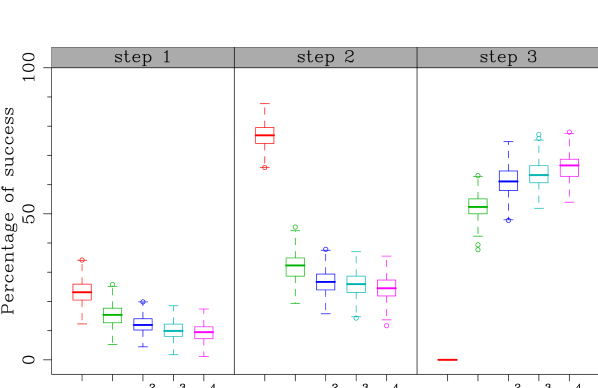
Figure 10: Box-and-whisker plot showing the percentage of success of the different steps described in Appendix A. The bottom and top of each box show the 25th and 75th percentiles, whereas the thick horizontal line marks the median. The whiskers (vertical dashed lines) show 1.5 times the interquartile range. Since each colour represents a fixed number of random points employed in the search for valid a blank field region in step 3, the sum of the percentages in the three steps for a fixed colour is 100.

References

- Bonnarel et al. (2000) Bonnarel, F., Fernique, P., Bienaymé, O., et al. 2000, A&AS, 143, 33
- Calabretta & Greisen (2002) Calabretta, M. R., & Greisen, E. W. 2002, A&A, 395, 1077
- Cepa et al. (2000) Cepa, J., et al. 2000, Proc. SPIE, 4008, 623
- Delaunay (1934) Delaunay B., 1934, Sur la sphère vide, Bull. Acad. Sci. USSR, 793–800
- Gilliland (1992) Gilliland R.L., 1992, Details of Noise Sources and Reduction Processes. In: Howell S.B. (ed.) ASP Conf. Ser. 23, Astronomical CCD Observing and Reduction Techniques, p. 68
- Høg et al. (2000) Høg, E., Fabricius, C., Makarov, V. V., et al. 2000, A&A, 355, L27
- Perryman et al. (1997) Perryman, M. A. C., Lindegren, L., Kovalevsky, J., et al. 1997, A&A, 323, L49
- Press et al. (2007) Press, W.H., Teukolsky, S.A., Vetterling, W.T., and Flannery, B.T., Numerical Recipes: The Art of Scientific Computing, 3rd ed., Cambridge Univ. Press, New York, 2007.
- Renka (1997) Renka R.J., 1997, Algorithm 772: STRIPACK: Delaunay Triangulation and Voronoi Diagram on the Surface of a Sphere, ACM Transactions on Mathematical Software, 23, 416–434
- Sinnott (1997) Sinnott, R. W. 1997, VizieR Online Data Catalog, VII/118, 0
-
Weisstein (2011)
Weisstein E.W. 2011, “Sphere Point Picking.´´ From MathWorld – A Wolfram Web Resource:
http://mathworld.wolfram.com/SpherePointPicking.html