Optimal control with stochastic PDE constraints and uncertain controls

Abstract

The optimal control of problems that are constrained by partial differential equations with uncertainties and with uncertain controls is addressed. The Lagrangian that defines the problem is postulated in terms of stochastic functions, with the control function possibly decomposed into an unknown deterministic component and a known zero-mean stochastic component. The extra freedom provided by the stochastic dimension in defining cost functionals is explored, demonstrating the scope for controlling statistical aspects of the system response. One-shot stochastic finite element methods are used to find approximate solutions to control problems. It is shown that applying the stochastic collocation finite element method to the formulated problem leads to a coupling between stochastic collocation points when a deterministic optimal control is considered or when moments are included in the cost functional, thereby forgoing the primary advantage of the collocation method over the stochastic Galerkin method for the considered problem. The application of the presented methods is demonstrated through a number of numerical examples. The presented framework is sufficiently general to also consider a class of inverse problems, and numerical examples of this type are also presented.

Keywords: Optimal control, uncertainty, stochastic finite element method, stochastic inverse problems, stochastic partial differential equations.

Introduction

In many applications, forces or boundary conditions are to be determined such that the response of a physical or engineering system is optimal in some sense. These problems can often be formulated as the minimisation of an objective functional subject to a set of constraint equations in the form of partial differential equations (PDEs). For problems that involve uncertainty, incorporating stochastic information into a control formulation can lead to a quantification of the statistics of the system response. Moreover, there is scope to control a system not only for an optimal mean response, but also to include statistics of the response in a cost functional. We note that stochastic PDE-constrained optimisation problems are closely related to stochastic inverse problems, where the control variable corresponds to the parameter to be identified [28, 13, 21].

We examine in this work the numerical solution of optimal control problems constrained by stochastic PDEs and with uncertain controls. Stochastic finite element-based solvers have been studied extensively for a large range of stochastic PDEs [24]. However, few results and examples on solving optimisation problems constrained by stochastic PDEs are available. Existence of an optimal solution to stochastic optimal control problems constrained by stochastic elliptic PDEs was studied by Hou et al. [12] for deterministic control functions. Borzì and von Winckel [7] and Borzì [5] studied multigrid solvers for stochastic collocation solutions of parabolic and elliptic optimal control problems with random coefficients and stochastic control functions. We contend that problems with an unknown stochastic ‘control function’ constitute stochastic inverse problems and are different from control problems where the focus is on computing a deterministic component of the control function which forms the control ‘signal’. If the stochastic properties of the control are computed, ad hoc procedures are required to extract a deterministic function, which will in general not be the optimal control. We choose to split the control function into an unknown deterministic component, which is to be computed, and a known zero-mean stochastic part that represents the uncertainty in the controller response.

Control cost functionals will be formulated in terms of norms that include both spatial and stochastic dimensions. The inclusion of the stochastic dimension provides additional freedom in the definition of cost functionals. We formulate a one-shot approach to control, and solve the resulting equations via a stochastic collocation or a Galerkin finite element method. The one-shot approach is in contrast with methods that require iteration [10]. Overviews of the stochastic collocation and Galerkin finite element methods can be found in [3] and [1], respectively. The stochastic collocation method is often preferred over the Galerkin approach as it converts a stochastic problem into a collection of decoupled deterministic problems. However, we will show that the so-called non-intrusivity property of the collocation method that is often exploited, including for stochastic inverse problems [28, 7], does not hold for a large class of stochastic PDE-constrained optimisation problems. The stochastic Galerkin method, on the other hand, can be applied straightforwardly to stochastic optimal control problems. The efficient solution of stochastic finite element problems, and in particular for the stochastic Galerkin method, can hinge on the development and application of effective preconditioners. This aspect is addressed for stochastic control problems, with two preconditioners that take the specific structure of the Galerkin one-shot systems into account presented. Extensive numerical examples support our investigations, and the computer code to reproduce all numerical results is available under the GNU Lesser Public License (LGPL) as part of the supporting material [20].

The remainder of this paper is organised as follows. Section 2 presents a control problem involving an elliptic stochastic PDE constraint and formulates this problem as a coupled system of stochastic PDEs. The framework developed in Section 2 is formulated such that it is sufficiently general to also address a class of inverse problems. The stochastic finite element discretisation is presented in Section 3. Section 4 considers additional regularising terms and their impact in the context of stochastic finite element solvers. Iterative solvers and preconditioners for the one-shot Galerkin system are discussed in Section 5, which is followed in Section 6 by numerical examples of stochastic optimal control problems. Numerical examples illustrating the solution of stochastic inverse problems are given in Section 7, and conclusions are drawn in Section 8.

A control problem with stochastic PDE constraints

We consider optimal control problems constrained by partial differential equations with stochastic coefficients. In general, these can be formulated as:

$$\min_{z\in Z,\>u\in U}\mathcal{J}(z,u)\quad\text{subject to}\quad c(z,u)=0,$$ (1)

where $\mathcal{J}\mathrel{\mathop{\mathchar 58\relax}}Z\times U\rightarrow\mathbb{R}$ is a cost (or objective) functional, $c$ is a constraint, $z$ the state variable, $u$ the control variable, and $Z$ and $U$ are suitably defined function spaces.

In this work, the constraint equations in (1) will be given by one or more PDEs with stochastic coefficients. The state variable will be a stochastic function and the control can be either deterministic or stochastic. Although the cost functional $\mathcal{J}$ contains stochastic functions, it will be defined such that its outcome is deterministic. Before presenting concrete examples, it is useful to provide some definitions.

Definitions

We will consider problems posed on a polygonal spatial domain $D\subset\mathbb{R}^{d}$ with boundary $\partial D$ and where $1\leq d\leq 3$. The boundary is decomposed into $\partial D_{D}$ and $\partial D_{N}$ such that $\partial D_{D}\cup\partial D_{N}=\partial D$ and $\partial D_{D}\cap\partial D_{N}=\emptyset$. The outward unit normal vector to $\partial D$ is denoted by $n$. Consider also a complete probability space $(\Omega,\mathcal{F},\mathcal{P})$, where $\Omega$ is a sample space, $\mathcal{F}$ is a $\sigma$-algebra and $\mathcal{P}$ is a probability measure. We define the tensor product Hilbert space $L^{2}(D)\otimes L^{2}(\Omega)$ of second-order random fields as

$$L^{2}(D)\otimes L^{2}(\Omega)=\mathinner{\left\{z\mathrel{\mathop{\mathchar 58\relax}}D\otimes\Omega\rightarrow\mathbb{R},\>\int_{\Omega}\int_{D}|z|^{2}\operatorname{d\!}x\operatorname{d\!}\mathcal{P}<\infty\right\}}.$$ (2)

This space is equipped with the norm

$$\mathinner{\!\left\lVert z\right\rVert}_{L^{2}(D)\otimes L^{2}(\Omega)}=\mathinner{\left(\int_{\Omega}\int_{D}|z|^{2}\operatorname{d\!}x\operatorname{d\!}\mathcal{P}\right)}^{\frac{1}{2}}.$$ (3)

Analogously, the tensor product spaces $H^{1}_{0}(D)\otimes L^{2}(\Omega)$ and $H^{1}(D)\otimes L^{2}(\Omega)$ can be defined [1].

Model problem

Constraint equation

As a model constraint, we consider a stochastic steady-state diffusion equation:

$$-\nabla_{x}\cdot\mathinner{\left(\kappa\mathinner{\left(x,\omega\right)}\nabla_{x}z\mathinner{\left(x,\omega\right)}\right)} =u\mathinner{\left(x,\omega\right)}\qquad x\in D,\ \omega\in\Omega,$$ (4)

$$z\mathinner{\left(x,\omega\right)} =z_{D}\mathinner{\left(x,\omega\right)}\qquad x\in\partial D_{D},\ \omega\in\Omega,$$ (5)

$$\kappa\mathinner{\left(x,\omega\right)}\nabla_{x}z\mathinner{\left(x,\omega\right)}\cdot n =g\mathinner{\left(x,\omega\right)}\qquad x\in\partial D_{N},\ \omega\in\Omega,$$ (6)

where the function $z\mathrel{\mathop{\mathchar 58\relax}}D\times\Omega\rightarrow\mathbb{R}$ is to be found, the diffusion coefficient $\kappa\mathrel{\mathop{\mathchar 58\relax}}D\times\Omega\rightarrow\mathbb{R}$ is prescribed, $u\mathrel{\mathop{\mathchar 58\relax}}D\times\Omega\rightarrow\mathbb{R}$ is a source term, $z_{D}\mathrel{\mathop{\mathchar 58\relax}}\partial D_{D}\times\Omega\rightarrow\mathbb{R}$ is a Dirichlet condition and $g\mathrel{\mathop{\mathchar 58\relax}}\partial D_{N}\times\Omega\rightarrow\mathbb{R}$ is a Neumann condition. The operator $\nabla_{x}$ involves only derivatives with respect to the spatial variable $x$. If $\kappa$, $u$, $z_{D}$ and $g$ are second-order random fields and assuming boundedness and positivity of the diffusion coefficient $\kappa$, existence and uniqueness of a weak solution $z$ can be proved [1].

In practice, for control problems $u$ and/or $g$ will not be prescribed, but computed as part of a constrained optimisation problem.

Cost functionals

We consider two cost functionals which, while outwardly similar, account differently for the stochastic nature of the problem. The first functional has the form:

$$\mathcal{J}_{1}\mathinner{\left(z,u,g\right)}\mathrel{\mathop{\mathchar 58\relax}}=\frac{\alpha}{2}\mathinner{\!\left\lVert z-\hat{z}\right\rVert}^{2}_{L^{2}(D)\otimes L^{2}(\Omega)}+\frac{\beta}{2}\mathinner{\!\left\lVert\mathrm{std}(z)\right\rVert}^{2}_{L^{2}(D)}\\ +\frac{\gamma}{2}\mathinner{\!\left\lVert u\right\rVert}^{2}_{L^{2}(D)\otimes L^{2}(\Omega)}+\frac{\delta}{2}\mathinner{\!\left\lVert g\right\rVert}^{2}_{L^{2}(\partial D_{N})\otimes L^{2}(\Omega)},$$ (7)

where $\hat{z}\mathrel{\mathop{\mathchar 58\relax}}D\times\Omega\rightarrow\mathbb{R}$ is a prescribed target function and $\alpha$, $\beta$, $\gamma$ and $\delta$ are positive constants. Typically for control problems $\hat{z}$ will be deterministic, but we permit here a more general case. The first term in (7) is a measure of the distance, between the state variable $z$ and the prescribed function $\hat{z}$, in terms of the expectation of $\mathinner{\left(z-\hat{z}\right)}^{2}$. The second term measures the standard deviation of $z$, which is denoted by $\mathrm{std}(z)$ and defined by:

$$\mathrm{std}(z)\mathrel{\mathop{\mathchar 58\relax}}=\mathinner{\left(\int_{\Omega}\mathinner{\left(z-\int_{\Omega}z\operatorname{d\!}\mathcal{P}\right)}^{2}\operatorname{d\!}\mathcal{P}\right)}^{\frac{1}{2}}.$$ (8)

By increasing the value of $\beta$ with respect to $\alpha$, a greater relative contribution of the variance of $z$ to $\mathcal{J}_{1}$ is implied. The final two terms in (7) are regularisation terms for the distributive control via $u$ and the boundary control via $g$.

The second considered functional has the form:

$$\mathcal{J}_{2}\mathinner{\left(z,u,g\right)}\mathrel{\mathop{\mathchar 58\relax}}=\frac{\alpha}{2}\mathinner{\!\left\lVert\bar{z}-\hat{z}\right\rVert}^{2}_{L^{2}(D)}+\frac{\beta}{2}\mathinner{\!\left\lVert\mathrm{std}(z)\right\rVert}^{2}_{L^{2}(D)}+\frac{\gamma}{2}\mathinner{\!\left\lVert u\right\rVert}^{2}_{L^{2}(D)\otimes L^{2}(\Omega)}+\frac{\delta}{2}\mathinner{\!\left\lVert g\right\rVert}^{2}_{L^{2}(\partial D_{N})\otimes L^{2}(\Omega)},$$ (9)

where $\bar{z}$ is the expectation of $z$ and $\hat{z}\mathrel{\mathop{\mathchar 58\relax}}D\rightarrow\mathbb{R}$ is a prescribed target function. This functional is subtly, but significantly, different from that in (7). The first term in $\mathcal{J}_{2}$ measures the $L^{2}$-distance between the expectation of $z$ and the target $\hat{z}$. This includes no measure of the variance of the actual response and is unaffected by the presence of uncertainty in $z$.

Setting $\alpha=1$, $\beta=0$ and $\delta=0$, the functional $\mathcal{J}_{1}$ in (7) coincides with a functional presented in Borzì [5], but in their work a method is constructed around a modified version of $\mathcal{J}_{1}$. For the above parameters and for deterministic $u$, $\mathcal{J}_{1}$ coincides with the cost functional considered by Hou et al. [12].

Structure of the control functions

A feature of our work is that for control problems, as opposed to inverse problems, we will consider control variables that are decomposed additively into unknown deterministic (to be computed) and known stochastic components. We will consider $u$ to have the form

$$u\mathinner{\left(x,\omega\right)}=\bar{u}\mathinner{\left(x\right)}+u^{\prime}\mathinner{\left(x,\omega\right)},$$ (10)

where $\bar{u}\mathrel{\mathop{\mathchar 58\relax}}D\rightarrow\mathbb{R}$ is deterministic and is the mean of $u$ and $u^{\prime}\mathrel{\mathop{\mathchar 58\relax}}D\times\Omega\rightarrow\mathbb{R}$ is a zero-mean stochastic part. The goal will be to compute $\bar{u}$, which constitutes the ‘signal’ sent to a control device. The actual controller response is $u$, with $u^{\prime}$ modelling the uncertainty in the controller response for a given instruction. The boundary control function will be decomposed analogously,

$$g\mathinner{\left(x,\omega\right)}=\bar{g}\mathinner{\left(x\right)}+g^{\prime}\mathinner{\left(x,\omega\right)},$$ (11)

where $\bar{g}\mathrel{\mathop{\mathchar 58\relax}}\partial D_{N}\rightarrow\mathbb{R}$ and $g^{\prime}\mathrel{\mathop{\mathchar 58\relax}}\partial D_{N}\times\Omega\rightarrow\mathbb{R}$ is a zero-mean stochastic part.

Representation of stochastic fields

Finite-dimensional noise assumption

In representing random fields, we employ the finite-dimensional noise assumption [1, Section 2.4], which states that the random fields $\kappa$, $z_{D}$, $g$ and $u$ can be approximated using a prescribed finite number of random variables $\xi=\mathinner{\left\{\xi_{i}\right\}}_{i=1}^{L}$, where $L\in\mathbb{N}$ and $\xi_{i}\mathrel{\mathop{\mathchar 58\relax}}\Omega\rightarrow\Gamma_{i}\subseteq\mathbb{R}$. We assume that each random variable is independent and is characterised by a probability density function $\rho_{i}\mathrel{\mathop{\mathchar 58\relax}}\Gamma_{i}\rightarrow[0,1]$. Defining the support $\Gamma=\prod_{i=1}^{L}\Gamma_{i}\subset\mathbb{R}^{L}$, for a given $y=(y_{1},\ldots,y_{L})\in\Gamma$ the joint probability density function of $\xi$ is given by $\rho=\prod_{i=1}^{L}\rho_{i}(y_{i})$. The preceding assumptions enable a parametrisation of the problem in $y$ in place of the random events $\omega$ [8].

As an example, consider a finite-term expansion of the stochastic coefficient $\kappa$ based on $L$ random variables:

$$\kappa(x,y)=\sum_{i=1}^{S}\kappa_{i}(x)\zeta_{i}(y)\qquad x\in D,\ y\in\Gamma,$$ (12)

where $\kappa_{i}\mathrel{\mathop{\mathchar 58\relax}}D\rightarrow\mathbb{R}$ and $\zeta_{i}\mathrel{\mathop{\mathchar 58\relax}}\Gamma\rightarrow\mathbb{R}$. If $\kappa$ is represented by a truncated Karhunen–Loève expansion [14], then $S=L+1$ with $\zeta_{i}=y_{i-1}$ and $y_{0}=1$. If a generalised polynomial chaos expansion [26] is used, $\zeta_{i}$ is an $L$-variate orthogonal polynomial of order $p$ and $S=(L+p)!/(L!p!)$.

Definitions

Given the joint probability density function $\rho(y)$ of $\xi$, with $y\in\Gamma$ and where $\Gamma$ is the support of $\rho$, a space $L^{2}_{\rho}(\Gamma)$ equipped with the inner product

$$(v,w)_{L^{2}_{\rho}(\Gamma)}\mathrel{\mathop{\mathchar 58\relax}}=\int_{\Gamma}vw\rho\operatorname{d\!}y\qquad v,w\in L^{2}_{\rho}(\Gamma)$$ (13)

is considered. The norm $\mathinner{\!\left\lVert\cdot\right\rVert}_{L^{2}(D)\otimes L^{2}_{\rho}(\Gamma)}$ is then defined as:

$$\mathinner{\!\left\lVert z\right\rVert}_{L^{2}(D)\otimes L^{2}_{\rho}(\Gamma)}\mathrel{\mathop{\mathchar 58\relax}}=\mathinner{\left(\int_{\Gamma}\int_{D}|z|^{2}\rho\operatorname{d\!}x\operatorname{d\!}y\right)}^{\frac{1}{2}}.$$ (14)

Expressing two functions $u_{1}$ and $u_{2}$ as $u_{1}(x,y)=v_{1}(x)w_{1}(y)$ and $u_{2}(x,y)=v_{2}(x)w_{2}(y)$, where $v_{1},v_{2}\in H^{1}(D)$ and $w_{1},w_{2}\in H^{1}_{\rho}(\Gamma)$, an inner product on $H^{1}(D)\otimes H^{1}_{\rho}(\Gamma)$ is defined by

$$\mathinner{\left(u_{1},u_{2}\right)}_{H^{1}(D)\otimes H^{1}_{\rho}(\Gamma)}\mathrel{\mathop{\mathchar 58\relax}}=\mathinner{\left(v_{1},v_{2}\right)}_{H^{1}(D)}\mathinner{\left(w_{1},w_{2}\right)}_{H^{1}_{\rho}(\Gamma)},$$ (15)

where $\mathinner{\left(\cdot,\cdot\right)}_{H^{1}(D)}$ is the standard $H^{1}$ inner product and $\mathinner{\left(\cdot,\cdot\right)}_{H^{1}_{\rho}}$ is the $H^{1}$ inner product weighted by $\rho$, analogous to (13). The norm $\mathinner{\!\left\lVert\cdot\right\rVert}_{H^{1}(D)\otimes H^{1}_{\rho}(\Gamma)}$ is that induced by (15). The $H^{1}$ definition will be used in Section 4 when considering the impact of introducing extra regularisation terms into the cost functionals.

Parametric optimal control problem

Following from the Doob–Dynkin Lemma [1], the random field $z$ can be expressed as a function of the given $L$ random variables. This enables one to reformulate the stochastic optimal control problem corresponding to the cost functional in (7) or (9) and the constraints in (4)–(6) as a parametric PDE-constrained optimisation problem. The parametric problem involves solving

$$\min_{z,u,g}\mathcal{J}_{1}\mathinner{\left(z,u,g\right)}\quad\text{or}\quad\min_{z,u,g}\mathcal{J}_{2}\mathinner{\left(z,u,g\right)}$$ (16)

subject to:

$$-\nabla_{x}\cdot\mathinner{\left(\kappa(x,y)\nabla_{x}z(x,y)\right)} =u(x,y)\quad x\in D,\ y\in\Gamma,$$ (17)

$$z(x,y) =z_{D}(x,y)\quad x\in\partial D_{D},\ y\in\Gamma,$$ (18)

$$\kappa(x,y)\nabla_{x}z(x,y)\cdot n =g(x,y)\quad x\in\partial D_{N},\ y\in\Gamma,$$ (19)

where

$$\mathcal{J}_{1}\mathinner{\left(z,u,g\right)}\mathrel{\mathop{\mathchar 58\relax}}=\frac{\alpha}{2}\mathinner{\!\left\lVert z-\hat{z}\right\rVert}^{2}_{L^{2}(D)\otimes L^{2}_{\rho}(\Gamma)}+\frac{\beta}{2}\mathinner{\!\left\lVert\mathrm{std}(z)\right\rVert}^{2}_{L^{2}(D)}\\ +\frac{\gamma}{2}\mathinner{\!\left\lVert u\right\rVert}^{2}_{L^{2}(D)\otimes L^{2}_{\rho}(\Gamma)}+\frac{\delta}{2}\mathinner{\!\left\lVert g\right\rVert}^{2}_{L^{2}(\partial D_{N})\otimes L^{2}_{\rho}(\Gamma)}$$ (20)

and

$$\mathcal{J}_{2}\mathinner{\left(z,u,g\right)}\mathrel{\mathop{\mathchar 58\relax}}=\frac{\alpha}{2}\mathinner{\!\left\lVert\bar{z}-\hat{z}\right\rVert}^{2}_{L^{2}(D)}+\frac{\beta}{2}\mathinner{\!\left\lVert\mathrm{std}(z)\right\rVert}^{2}_{L^{2}(D)}+\frac{\gamma}{2}\mathinner{\!\left\lVert u\right\rVert}^{2}_{L^{2}(D)\otimes L^{2}_{\rho}(\Gamma)}+\frac{\delta}{2}\mathinner{\!\left\lVert g\right\rVert}^{2}_{L^{2}(\partial D_{N})\otimes L^{2}_{\rho}(\Gamma)}.$$ (21)

This parametric form of the problem will be considered in the remainder.

One-shot solution approach

The PDE-constrained optimisation problem in (16)–(19) can be recast as an unconstrained optimisation problem by following the standard procedure of introducing Lagrange multipliers [10, 23]. By defining a Lagrangian functional, optimality conditions can be formulated for the state, control and adjoint variables [23] and these can be solved simultaneously. This so-called ‘one-shot’ approach yields a solution for an optimal control problem without having to apply iterative optimisation routines.

Lagrangian functionals

Introducing adjoint variables, or Lagrange multipliers, $\lambda,\chi\in H_{0}^{1}(D)\otimes L^{2}_{\rho}(\Gamma)$, we define a Lagrangian associated with the cost functional $\mathcal{J}_{1}$ in (20) and the constraints (17)–(19) as:

$$\mathcal{L}_{1}(z,u,g,\lambda,\chi)\mathrel{\mathop{\mathchar 58\relax}}=\frac{\alpha}{2}\int_{\Gamma}\int_{D}\mathinner{\left(z-\hat{z}\right)}^{2}\rho\operatorname{d\!}x\operatorname{d\!}y+\frac{\beta}{2}\int_{\Gamma}\int_{D}z^{2}\rho\operatorname{d\!}x\operatorname{d\!}y-\frac{\beta}{2}\int_{D}\mathinner{\left(\int_{\Gamma}z\rho\operatorname{d\!}y\right)}^{2}\operatorname{d\!}x\\ +\frac{\gamma}{2}\int_{\Gamma}\int_{D}u^{2}\rho\operatorname{d\!}x\operatorname{d\!}y+\frac{\delta}{2}\int_{\Gamma}\int_{\partial D_{N}}g^{2}\rho\operatorname{d\!}s\operatorname{d\!}y-\int_{\Gamma}\int_{D}\lambda\mathinner{\left(-\nabla_{x}\cdot\mathinner{\left(\kappa\nabla_{x}z\right)}-u\right)}\rho\operatorname{d\!}x\operatorname{d\!}y\\ -\int_{\Gamma}\int_{\partial D_{N}}\chi\mathinner{\left(\kappa\frac{dz}{dn}-g\right)}\rho\operatorname{d\!}s\operatorname{d\!}y.$$ (22)

A Lagrange multiplier has not been introduced to impose the Dirichlet boundary condition in (18) since this condition will be imposed by construction via the definition of the function space to which $z$ belongs. For the problem associated with the cost functional $\mathcal{J}_{2}$ in (21), we define the Lagrangian

$$\mathcal{L}_{2}(z,u,g,\lambda,\chi)\mathrel{\mathop{\mathchar 58\relax}}=\frac{\alpha}{2}\int_{D}\mathinner{\left(\int_{\Gamma}z\rho\operatorname{d\!}y-\hat{z}\right)}^{2}\operatorname{d\!}x+\frac{\beta}{2}\int_{\Gamma}\int_{D}z^{2}\rho\operatorname{d\!}x\operatorname{d\!}y-\frac{\beta}{2}\int_{D}\mathinner{\left(\int_{\Gamma}z\rho\operatorname{d\!}y\right)}^{2}\operatorname{d\!}x\\ +\frac{\gamma}{2}\int_{\Gamma}\int_{D}u^{2}\rho\operatorname{d\!}x\operatorname{d\!}y+\frac{\delta}{2}\int_{\Gamma}\int_{\partial D_{N}}g^{2}\rho\operatorname{d\!}s\operatorname{d\!}y-\int_{\Gamma}\int_{D}\lambda\mathinner{\left(-\nabla_{x}\cdot\mathinner{\left(\kappa\nabla_{x}z\right)}-u\right)}\rho\operatorname{d\!}x\operatorname{d\!}y\\ -\int_{\Gamma}\int_{\partial D_{N}}\chi\mathinner{\left(\kappa\frac{dz}{dn}-g\right)}\rho\operatorname{d\!}s\operatorname{d\!}y.$$ (23)

The control problems that we wish to solve involve finding stationary points of these Lagrangians. The existence of Lagrange multipliers for stochastic optimal control problems is proved by Hou et al. [12] for $\mathcal{J}_{1}$ with $\alpha=1$, $\beta=0$ and $\delta=0$. The result extends to the more general form of $\mathcal{J}_{1}$ because of the Fréchet differentiability of $\mathinner{\!\left\lVert\mathrm{std}(z)\right\rVert}^{2}_{L^{2}(D)}$ and $\mathinner{\!\left\lVert g\right\rVert}^{2}_{L^{2}(\partial D_{N})\otimes L^{2}_{\rho}(\Gamma)}$.

Optimality system

To find stationary points of the Lagrangians in (22) and (23), we consider variations with respect to the adjoint, state and control variables. This will lead to the first-order optimality conditions, which are known as the state, adjoint and optimality system of equations [10]. In the remainder of this section, these equations are derived by setting the directional derivative of the Lagrangians with respect to the adjoint, state and control variable, respectively, equal to zero.

Following standard variational arguments, taking the directional derivative of $\mathcal{L}_{1}$ or of $\mathcal{L}_{2}$ with respect to $\chi$ and setting this equal to zero for all variations leads to the recovery of the Neumann boundary condition in (19). Likewise, taking directional derivatives with respect to $\lambda$ and setting this equal to zero for all variations leads to the recovery of the constraint equation in (17). The state system of equations corresponds thus to the constraint equations (17)–(19).

The derivative of $\mathcal{L}_{1}$ with respect to the state variable $z$ in the direction of $z^{\star}\in H^{1}_{0}(D)\otimes L^{2}_{\rho}(\Gamma)$ reads:

$$\mathcal{L}_{1,z}\mathinner{\left[z^{\star}\right]}=\alpha\int_{\Gamma}\int_{D}(z-\hat{z})z^{\star}\rho\operatorname{d\!}x\operatorname{d\!}y+\beta\int_{\Gamma}\int_{D}zz^{\star}\rho\operatorname{d\!}x\operatorname{d\!}y-\beta\int_{\Gamma}\int_{D}\mathinner{\left(\int_{\Gamma}z\rho\operatorname{d\!}y\right)}z^{\star}\rho\operatorname{d\!}x\operatorname{d\!}y\\ +\int_{\Gamma}\int_{D}\lambda\nabla_{x}\cdot(\kappa\nabla_{x}z^{\star})\rho\operatorname{d\!}x\operatorname{d\!}y-\int_{\Gamma}\int_{\partial D_{N}}\chi\kappa\frac{dz^{\star}}{dn}\rho\operatorname{d\!}s\operatorname{d\!}y.$$ (24)

Setting $\mathcal{L}_{1,z}\mathinner{\left[z^{\star}\right]}=0$ for all $z^{\star}$ and following standard arguments, the following adjoint system of equations can be deduced:

$$-\nabla_{x}\cdot(\kappa(x,y)\nabla_{x}\lambda(x,y)) =(\alpha+\beta)z(x,y)-\alpha\hat{z}(x,y)-\beta\int_{\Gamma}z\rho\operatorname{d\!}y x\in D,\>y\in\Gamma,$$ (25)

$$\kappa(x,y)\nabla_{x}\lambda(x,y)\cdot n =0 x\in\partial D_{N},\>y\in\Gamma,$$ (26)

$$\lambda(x,y) =0 x\in\partial D_{D},\>y\in\Gamma,$$ (27)

$$\lambda(x,y) =\chi(x,y) x\in\partial D_{N},\>y\in\Gamma.$$ (28)

The last equation $\lambda=\chi$ is trivial. For distributive control via $u$ the directional derivative of $\mathcal{L}_{1}$ with respect to $u$ in the direction of $u^{\star}\in L^{2}(D)\otimes L^{2}_{\rho}(\Gamma)$ reads:

$$\mathcal{L}_{1,u}\mathinner{\left[u^{\star}\right]}=\int_{\Gamma}\int_{D}(\gamma u+\lambda)u^{\star}\rho\operatorname{d\!}x\operatorname{d\!}y.$$ (29)

Setting the above equal to zero for all $u^{\star}$ implies that

$$\gamma u(x,y)+\lambda(x,y)=0\qquad x\in D,\>y\in\Gamma.$$ (30)

More specifically, considering the structure of $u$ in (10), in which only the mean $\bar{u}$ is unknown, the optimality equation reads:

$$\gamma\bar{u}(x)+\int_{\Gamma}\mathinner{\left(\gamma u^{\prime}+\lambda\right)}\rho\operatorname{d\!}y=0.$$ (31)

Since the mean of $u^{\prime}$ is zero, this optimality condition reduces to

$$\gamma\bar{u}(x)+\int_{\Gamma}\lambda\rho\operatorname{d\!}y=0\qquad x\in D.$$ (32)

The case of a boundary control is handled in the same fashion, but is omitted for brevity.

The optimality conditions in (30) and (32) permit the expression of the control ($u$ or $\bar{u}$) as a function of the adjoint function $\lambda$. The control can be eliminated from the first-order optimality equations, leaving a reduced optimality system in terms of the state and adjoint variables. In summary, the optimal control problem involves solving the parametric constraint problem (17)–(19), with $u$ or $\bar{u}$ eliminated using (30) or (32), and the parametric adjoint problem (25)–(27).

The reduced optimality system corresponding to $\mathcal{L}_{2}$ is constructed in the same fashion as for $\mathcal{L}_{1}$. It consists of the parametric constraint problem in (17)–(19), with $u$ or $\bar{u}$ eliminated using (30) or (32), and a parametric adjoint problem that reads:

$$-\nabla_{x}\cdot(\kappa(x,y)\nabla_{x}\lambda(x,y)) =\beta z(x,y)-\alpha\hat{z}(x,y)+(\alpha-\beta)\int_{\Gamma}z\rho\operatorname{d\!}y x\in D,\>y\in\Gamma,$$ (33)

$$\kappa(x,y)\nabla_{x}\lambda(x,y)\cdot n =0 x\in\partial D_{N},\>y\in\Gamma,$$ (34)

$$\lambda(x,y) =0 x\in\partial D_{D},\>y\in\Gamma.$$ (35)

Stochastic finite element solution

To compute approximate solutions to the optimality system derived in Section 2.4.2, both a stochastic Galerkin and a stochastic collocation finite element discretisation are formulated. For brevity, we present the formulation for distributive control only. The boundary control case, which is considered in the examples section, is formulated analogously.

For both the stochastic Galerkin and stochastic collocation methods, for the spatial domain we define a space $V_{h}\subset H^{1}_{0}(D)$ of standard Lagrange finite element functions on a triangulation $\mathcal{T}$ of the domain $D$:

$$V_{h}\mathrel{\mathop{\mathchar 58\relax}}=\mathinner{\left\{v_{h}\in H^{1}_{0}(D)\mathrel{\mathop{\mathchar 58\relax}}v_{h}\in P_{k}(K)\ \forall\ K\in\mathcal{T}\right\}},$$ (36)

where $K\in\mathcal{T}$ is a cell and $P_{k}$ is the space of Lagrange polynomials of degree $k$. The space $V_{h}$ is spanned by the basis functions $\mathinner{\left\{\phi_{i}\right\}}_{i=1}^{N}$.

Stochastic Galerkin finite element method

To develop a stochastic Galerkin finite element formulation, we consider a finite dimensional space $Y_{p}\subset L_{\rho}^{2}\mathinner{\left(\Gamma\right)}$ for the stochastic dimension. For $Y_{p}$, we adopt a polynomial basis, also known as a generalised polynomial chaos [24, 9]. We first consider multivariate polynomials $\psi_{q}\mathrel{\mathop{\mathchar 58\relax}}\Gamma\rightarrow\mathbb{R}$ generated via [16]

$$\psi_{q}=\prod_{i=1}^{L}\varphi_{q_{i}}(y_{i}),$$ (37)

where $q=\mathinner{\left(q_{1},\ldots,q_{L}\right)}\in\mathbb{N}^{L}$ is a multi-index that satisfies $|q|\leq p$ and $\varphi_{q_{i}}\mathrel{\mathop{\mathchar 58\relax}}\Gamma_{q_{i}}\rightarrow\mathbb{R}$ is a one-dimensional orthogonal polynomial of degree $q_{i}$. Note that $p$ is the prescribed total polynomial degree and recall that $L$ is the number of random variables in the problem. The polynomials $\psi_{q}$ are orthonormal with respect to the $L^{2}_{\rho}(\Gamma)$-inner product defined in (13). The space $Y_{p}$ is defined in terms of $\psi_{q}$:

$$Y_{p}\mathrel{\mathop{\mathchar 58\relax}}={\rm span}\mathinner{\left\{\psi_{q}\mathrel{\mathop{\mathchar 58\relax}}q\in\mathcal{M}\right\}}\subset L_{\rho}^{2}(\Gamma),$$ (38)

where $\mathcal{M}$ is the set of all multi-indices of length $L$ that satisfy $|q|\leq p$ for $q\in\mathcal{M}$. It holds that $\dim\mathinner{\left(Y_{p}\right)}=\dim\mathinner{\left(\mathcal{M}\right)}=Q=\binom{L+p}{L}=(L+p)!/(L!p!)$. Consequently, there exists a bijection

$$\mu\mathrel{\mathop{\mathchar 58\relax}}\mathinner{\left\{1,\ldots,Q\right\}}\rightarrow\mathcal{M}$$ (39)

that assigns a unique integer $j$ to each multi-index $\mu(j)\in\mathcal{M}$.

A function $z_{hp}\in V_{h}\otimes Y_{p}$ is represented as

$$z_{hp}(x,y)=\sum_{i=1}^{N}\sum_{q\in\mathcal{M}}z_{i,q}\phi_{i}(x)\psi_{q}(y),$$ (40)

where $z_{i,q}$ is a degree of freedom (recall that $V_{h}$ is spanned by $\mathinner{\left\{\phi_{i}\right\}}_{i=1}^{N}$). Using the above, for the case of the cost functional $\mathcal{J}_{1}$ with unknown stochastic $u$, a Galerkin formulation of the optimality conditions reads: find $z_{hp}\in V_{h}\otimes Y_{p}$ and $\lambda_{hp}\in V_{h}\otimes Y_{p}$ such that

$$\int_{\Gamma}\int_{D}\kappa\nabla_{x}z_{hp}\cdot\nabla_{x}w_{hp}\rho\operatorname{d\!}x\operatorname{d\!}y+\frac{1}{\gamma}\int_{\Gamma}\int_{D}\lambda_{hp}w_{hp}\rho\operatorname{d\!}x\operatorname{d\!}y\\ =\int_{\Gamma}\int_{\partial D_{N}}gw_{hp}\rho\operatorname{d\!}s\operatorname{d\!}y\quad\forall\ w_{hp}\in V_{h}\otimes Y_{p}$$ (41)

and

$$\int_{\Gamma}\int_{D}\kappa\nabla_{x}\lambda_{hp}\cdot\nabla_{x}r_{hp}\rho\operatorname{d\!}x\operatorname{d\!}y-\mathinner{\left(\alpha+\beta\right)}\int_{\Gamma}\int_{D}z_{hp}r_{hp}\rho\operatorname{d\!}x\operatorname{d\!}y\\ +\beta\int_{D}\mathinner{\left(\int_{\Gamma}z_{hp}\rho\operatorname{d\!}y\right)}\mathinner{\left(\int_{\Gamma}r_{hp}\rho\operatorname{d\!}y\right)}\operatorname{d\!}x=-\alpha\int_{\Gamma}\int_{D}\hat{z}r_{hp}\rho\operatorname{d\!}x\operatorname{d\!}y\quad\forall\ r_{hp}\in V_{h}\otimes Y_{p}.$$ (42)

For the case that $u$ is decomposed additively according to (10) and only $\bar{u}$ is to be computed, equation (41) is replaced by:

$$\int_{\Gamma}\int_{D}\kappa\nabla_{x}z_{hp}\cdot\nabla_{x}w_{hp}\rho\operatorname{d\!}x\operatorname{d\!}y+\frac{1}{\gamma}\int_{D}\mathinner{\left(\int_{\Gamma}\lambda_{hp}\rho\operatorname{d\!}y\right)}\mathinner{\left(\int_{\Gamma}w_{hp}\rho\operatorname{d\!}y\right)}\operatorname{d\!}x\\ =\int_{\Gamma}\int_{D}u^{\prime}w_{hp}\rho\operatorname{d\!}x\operatorname{d\!}y+\int_{\Gamma}\int_{\partial D_{N}}gw_{hp}\rho\operatorname{d\!}s\operatorname{d\!}y.$$ (43)

It can be helpful to examine the structure of the matrix systems that result from the above finite element problems. The space $V_{h}$ is spanned by $N$ nodal basis functions, with $N$ the number of spatial degrees of freedom. This enables the construction of a mass matrix $M\in\mathbb{R}^{N\times N}$ and a set of stiffness matrices $K_{i}\in\mathbb{R}^{N\times N}$, $i=1,\ldots,S$, with each corresponding to a deterministic diffusion coefficient $\kappa_{i}$ in (12). The space $Y_{p}$ is spanned by $Q$ polynomials and the stochastic discretisation of $\kappa$ in (12) defines a set of matrices $C_{i}\in\mathbb{R}^{Q\times Q}$, $i=1,\ldots,S$, whose elements equal

$$C_{i}(j,k)\mathrel{\mathop{\mathchar 58\relax}}=\int_{\Gamma}\zeta_{i}\psi_{\mu(j)}\psi_{\mu(k)}\rho\operatorname{d\!}y\quad\mathrm{for}\ j,k=1,\ldots,Q.$$ (44)

The resulting matrix formulation of the finite element problem in (41) and (42) is then given by:

$$\mathinner{\left(\sum_{i=1}^{S}\begin{bmatrix}C_{i}&\bm{0}_{Q}\\ \bm{0}_{Q}&C_{i}\end{bmatrix}\otimes K_{i}+\begin{bmatrix}\bm{0}_{Q}&T\mathinner{\left(\frac{1}{\gamma},\frac{-\epsilon}{\gamma}\right)}\\ T(-\alpha,-\beta)&\bm{0}_{Q}\end{bmatrix}\otimes M\right)}\begin{bmatrix}\bm{z}_{1}\\ \ldots\\ \bm{z}_{Q}\\ \bm{\lambda}_{1}\\ \ldots\\ \bm{\lambda}_{Q}\end{bmatrix}=\begin{bmatrix}\bm{g}_{1}+\epsilon\bm{u}^{\prime}_{1}\\ \ldots\\ \bm{g}_{Q}+\epsilon\bm{u}^{\prime}_{Q}\\ -\alpha\bm{\hat{z}}_{1}\\ \ldots\\ -\alpha\bm{\hat{z}}_{Q}\end{bmatrix},$$ (45)

where $\epsilon=0$ in the case of a stochastic control $u$ (see (41)) and $\epsilon=1$ when only $\bar{u}$ is unknown (see (43)). The matrix $\bm{0}_{Q}\in\mathbb{R}^{Q\times Q}$ is a zero matrix. The diagonal matrix $T\in\mathbb{R}^{Q\times Q}$ is defined as:

$$T(a,b)\mathrel{\mathop{\mathchar 58\relax}}=\mathrm{diag}\mathinner{\left(\begin{bmatrix}a&a+b&\ldots&a+b\end{bmatrix}^{T}\right)}.$$ (46)

The vectors $\bm{z}_{q},\,\bm{\lambda}_{q}\in\mathbb{R}^{N}$, with $q=1,\ldots,Q$, collect the spatial degrees of freedom of $z_{hp}$ and $\lambda_{hp}$, respectively, in (40); the vectors $\bm{\hat{z}}_{q},\bm{g}_{q},\,\bm{u}^{\prime}_{q}\in\mathbb{R}^{N}$ represent the finite element discretisation of $\int_{\Gamma}\int_{D}\hat{z}\psi_{q}\rho\operatorname{d\!}x\operatorname{d\!}y$, $\int_{\Gamma}\int_{\partial D_{N}}g\psi_{q}\rho\operatorname{d\!}s\operatorname{d\!}y$ and $\int_{\Gamma}\int_{D}u^{\prime}\psi_{q}\rho\operatorname{d\!}x\operatorname{d\!}y$, respectively.

Stochastic collocation finite element method

In applying the stochastic collocation method [2, 25], we solve the optimality system at a collection of collocation points $\mathinner{\left\{\hat{y}^{i}\right\}}_{i=1}^{Q}$, where $\hat{y}^{i}\in\Gamma$. Typically, the collocation points are determined by constructing a sparse grid, see [3, 4] for details on the point selection. Of relevance at this stage is that integrals of the form $\int_{\Gamma}\mathinner{\left(\cdot\right)}\rho\operatorname{d\!}y$ can be approximated via

$$\int_{\Gamma}z(x,y)\rho dy\approx\sum_{i=1}^{Q}z(x,\hat{y}^{i})w_{i},$$ (47)

where $w_{i}$ is an appropriate cubature weight and $Q$ is the number of cubature points.

From the $Q$ realisations $\mathinner{\left\{z_{i}=z(x,\hat{y}^{i})\right\}}_{i=1}^{Q}$, a semi-discrete global approximation of the response can be constructed,

$$z_{p}(x,y)=\sum_{i=1}^{Q}z(x,\hat{y}^{i})\widetilde{\psi}_{i}(y),$$ (48)

where the multivariate polynomials $\widetilde{\psi}_{i}$ are commonly interpolatory Lagrange polynomials, as defined in Babuška et al. [3]. The polynomial representation permits an exact evaluation of the expectation of $z_{p}$ by the cubature rule (47) when the order of the cubature rule is sufficiently high [25]. Other moments of the response, as well its probability density function, can be easily extracted using a cubature rule and the expansion in (48).

The main computational cost of the stochastic collocation method is associated with solving the optimality system at each collocation point. That is, for each $\hat{y}^{i}$, $i=1,\ldots,Q$, the state equation (17)–(19),

$$-\nabla_{x}\cdot\mathinner{\left(\kappa(x,\hat{y}^{i})\nabla_{x}z(x,\hat{y}^{i})\right)} =u(x,\hat{y}^{i}) \mathrm{on}\ D,$$ (49)

$$z(x,\hat{y}^{i}) =z_{D}(x,\hat{y}^{i}) \mathrm{on}\ \partial D_{D},$$ (50)

$$\kappa(x,\hat{y}^{i})\nabla_{x}z(x,\hat{y}^{i})\cdot n =g(x,\hat{y}^{i}) \mathrm{on}\ \partial D_{N},$$ (51)

and the adjoint problem (25)–(28),

$$-\nabla_{x}\cdot\mathinner{\left(\kappa(x,\hat{y}^{i})\nabla_{x}\lambda(x,\hat{y}^{i})\right)} =(\alpha+\beta)z(x,\hat{y}^{i})-\alpha\hat{z}(x,\hat{y}^{i})-\beta\sum_{j=1}^{Q}z(x,\hat{y}^{j})w_{j} \mathrm{on}\ D,$$ (52)

$$\kappa(x,\hat{y}^{i})\nabla_{x}\lambda(x,\hat{y}^{i})\cdot n =0 \mathrm{on}\ \partial D_{N},$$ (53)

$$\lambda(x,\hat{y}^{i}) =0 \mathrm{on}\ \partial D_{D},$$ (54)

are solved. For the case that the unknown control $u$ is wholly stochastic, equation (30) is used to eliminate $u$ in favour of $\lambda$:

$$u(x,\hat{y}^{i})=-\frac{1}{\gamma}\lambda(x,\hat{y}^{i}).$$ (55)

If the control function has the additive structure of (10), then

$$\bar{u}(x)=-\frac{1}{\gamma}\sum_{j=1}^{Q}\lambda(x,\hat{y}^{j})w_{j},$$ (56)

is used. This equation corresponds to the case where only the mean part $\bar{u}$ in (10) is to be computed and the stochastic part $u^{\prime}$ is prescribed.

Remark 3.1.

When moments of unknown functions, e.g., the expectation or standard deviation, appear in the control problem, the $Q$ sets of equations in the stochastic collocation method become coupled. For the case that $u=\bar{u}+u^{\prime}$, the state equation (49) is of the form

$$-\nabla_{x}\cdot\mathinner{\left(\kappa(x,\hat{y}^{i})\nabla_{x}z(x,\hat{y}^{i})\right)}=\bar{u}(x)+u^{\prime}(x,\hat{y}^{i}),$$ (57)

where $u^{\prime}(x,\hat{y}^{i})$ is known. Following the usual process of applying equation (56) to eliminate the control function $\bar{u}$ in the constraint equation (57) in favour of the adjoint variable $\lambda$, the $Q$ deterministic problems become coupled via this term. A similar coupling is observed for $\beta\neq 0$ in (52) and $\alpha\neq 0$ in (33). The advantage of decoupled systems of equations that is usually associated with the stochastic collocation method is therefore lost.

Once the collocation systems are solved, the cost functional $\mathcal{J}_{1}$ can be evaluated as follows:

$$\mathcal{J}_{1}(z,u,g)=\sum_{i=1}^{Q}w_{i}\int_{D}z_{i}\mathinner{\left(\frac{\alpha+\beta}{2}z_{i}-\alpha\hat{z}-\frac{\beta}{2}\sum_{j=1}^{Q}z_{j}\right)}\operatorname{d\!}x+\frac{\alpha}{2}\int_{D}\hat{z}^{2}\operatorname{d\!}x\\ +\frac{\gamma}{2}\sum_{i=1}^{Q}w_{i}\int_{D}u_{i}^{2}\operatorname{d\!}x+\frac{\delta}{2}\sum_{i=1}^{Q}w_{i}\int_{\partial D_{N}}g_{i}^{2}\operatorname{d\!}s,$$ (58)

with $u_{i}=u(x,\hat{y}^{i})$ and $g_{i}=g(x,\hat{y}^{i})$. The scalars $w_{i}$, $i=1,\ldots,Q$, represent the cubature weights corresponding to the cubature points $\mathinner{\left\{\hat{y}^{i}\right\}}_{i=1}^{Q}$, see (47). The cost functional $\mathcal{J}_{2}$ can be likewise evaluated.

The coupling of the collocation systems can be visualised through a matrix formulation. Following from the finite element space $V_{h}$, we define a mass matrix $M\in\mathbb{R}^{N\times N}$ and a set of stiffness matrices $K_{i}\in\mathbb{R}^{N\times N}$, $i=1,\ldots,Q$, each corresponding to a $\kappa(x,\hat{y}^{i})$. For a distributive control function $u$ ($\delta=0$ in (20)), the matrix formulation of the stochastic collocation finite element systems in (49)–(56) reads:

$$\begin{bmatrix}K_{1}&&&\frac{1}{\gamma}M&\frac{\epsilon}{\gamma}M\>\ldots&\frac{\epsilon}{\gamma}M\\ &\ddots&&\frac{\epsilon}{\gamma}M&\ddots&\vdots\\ &&K_{Q}&\vdots&\ldots\>\frac{\epsilon}{\gamma}M&\frac{1}{\gamma}M\\ &&&K_{1}&&\\ \lx@intercol\hfil\mathinner{\left(-(\alpha+\beta)I_{Q}+\beta\mathinner{\left(\mathbf{1}\mathbf{w}^{T}\right)}\right)}\otimes M\hfil\lx@intercol&&\ddots&\\ &&&&&K_{Q}\end{bmatrix}\begin{bmatrix}\bm{z}_{1}\\ \vdots\\ \bm{z}_{Q}\\ \bm{\lambda}_{1}\\ \vdots\\ \bm{\lambda}_{Q}\end{bmatrix}=\begin{bmatrix}\bm{g}_{1}+\epsilon\bm{u}^{\prime}_{1}\\ \ldots\\ \bm{g}_{Q}+\epsilon\bm{u}^{\prime}_{Q}\\ -\alpha\bm{\hat{z}}_{1}\\ \ldots\\ -\alpha\bm{\hat{z}}_{Q}\end{bmatrix},$$ (59)

where $\epsilon=0$ for the case that $u$ is wholly stochastic (see (55)) and $\epsilon=1$ when only $\bar{u}$ is unknown (see (56)). The vectors $\bm{z}_{i},\,\bm{\lambda_{i}},\,\bm{\hat{z}}_{i},\,\bm{g}_{i},\,\bm{u}^{\prime}_{i}\in\mathbb{R}^{N}$, with $i=1,\ldots,Q$, are the finite element representations of $z(x,\hat{y}^{i})$, $\lambda(x,\hat{y}^{i})$, $\hat{z}(x,\hat{y}^{i})$, $g(x,\hat{y}^{i})$ and $u^{\prime}(x,\hat{y}^{i})$, respectively. The matrix $I_{Q}\in\mathbb{R}^{Q\times Q}$ is an identity matrix and the vectors $\mathbf{1},\mathbf{w}\in\mathbb{R}^{Q}$ are defined by $[1\ \ldots\ 1]^{T}$ and $[w_{1}\ \ldots\ w_{Q}]^{T}$, respectively.

In contrast with the stochastic inverse type problems in Borzì and von Winckel [7] and Zabaras and Ganapathysubramanian [28] to which the non-intrusivity property of the stochastic collocation method is preserved, deterministic simulation software cannot readily be reused for $\beta\neq 0$ or $\epsilon\neq 0$.

Remark 3.2.

The stochastic collocation method generally requires more stochastic degrees of freedom, i.e., a larger $Q$, than the stochastic Galerkin method in order to solve a stochastic PDE to the same accuracy [4]. Therefore, for the same accuracy, due to the coupling of the stochastic collocation systems (see (59)) the stochastic collocation method will likely involve a greater computational cost compared to the stochastic Galerkin method. When presenting numerical examples, we will therefore only apply the stochastic collocation method to problems for which the non-intrusivity of the stochastic collocation method is maintained, i.e., only for the cost functional $\mathcal{J}_{1}$ with unknown stochastic $u$ and $\beta=0$.

Additional regularisation of stochastic optimal control problems

The cost functionals $\mathcal{J}_{1}$ and $\mathcal{J}_{2}$ both contain a regularisation term of the form $(\gamma/2)\mathinner{\!\left\lVert u\right\rVert}^{2}_{L^{2}(D)\otimes L^{2}(\Omega)}$. This $L^{2}$-regularisation is important for the solvability of the problem, and as $\gamma$ is increased excessive control values are penalised [11]. However, in some applications $L^{2}$-penalisation may not be sufficient. We detail in this section how an additional $H^{1}$-like regularisation can be included into the cost functionals and show what computational issues then follow.

Assuming sufficient regularity of the relevant functions, we extend the functional $\mathcal{J}_{1}$ in (7) by including a $H^{1}$-penalty on the control variables:

$$\mathcal{J}_{1,H^{1}}\mathinner{\left(z,u,g\right)}\mathrel{\mathop{\mathchar 58\relax}}=\frac{\alpha}{2}\mathinner{\!\left\lVert z-\hat{z}\right\rVert}^{2}_{L^{2}(D)\otimes L^{2}_{\rho}(\Gamma)}+\frac{\beta}{2}\mathinner{\!\left\lVert\mathrm{std}(z)\right\rVert}^{2}_{L^{2}(D)}\\ +\frac{\gamma}{2}\mathinner{\!\left\lVert u\right\rVert}^{2}_{H^{1}(D)\otimes H^{1}_{\rho}(\Gamma)}+\frac{\delta}{2}\mathinner{\!\left\lVert g\right\rVert}^{2}_{H^{1}(\partial D_{N})\otimes H^{1}_{\rho}(\Gamma)}.$$ (60)

A stochastic optimal control problem involving the cost functional $\mathcal{J}_{1,H^{1}}$ and the PDE constraints in (17)–(19) can be solved by following the one-shot strategy described in Section 2.4. The state equations are given by (17)–(19) and the adjoint equations are given by (25)–(28) (see Section 2.4.2). For the distributive control $u$, the weak optimality condition for the $\mathcal{J}_{1,H^{1}}$ case reads:

$$\int_{\Gamma}\int_{D}\lambda u^{\star}\rho\operatorname{d\!}x\operatorname{d\!}y+\gamma\mathinner{\left(u,u^{\star}\right)}_{H^{1}(D)\otimes H^{1}_{\rho}(\Gamma)}=0$$ (61)

for all $u^{\star}\in H^{1}(D)\otimes H^{1}_{\rho}(\Gamma)$. For the additive structure of $u$ in (10), in which only the mean $\bar{u}$ is unknown, the weak optimality condition reduces to

$$\gamma\int_{D}\bar{u}u^{\star}+\nabla_{x}\bar{u}\cdot\nabla_{x}u^{\star}\operatorname{d\!}x+\int_{\Gamma}\int_{D}\lambda u^{\star}\rho\operatorname{d\!}x\operatorname{d\!}y=0$$ (62)

for all $u^{\star}\in H^{1}(D)$, in which the zero-mean property of $u^{\prime}$ has been used. In contrast with the optimality conditions in (30) and (32), the optimality conditions (61) and (62) are partial differential equations and do not permit the straightforward expression of the control function as a function of the adjoint field $\lambda$. As a result, no reduced optimality system is constructed and the optimality equations for the state, control and adjoint variables will be solved simultaneously.

The Galerkin formulation of the optimality system is composed of three equations, which are the Galerkin formulation of the constraint equations (17)–(19), the Galerkin formulation of the adjoint equations (25)–(28), see (42), and the optimality condition in (61) or (62). Some structure of the stochastic Galerkin method can be revealed from its matrix formulation. When the unknown control $u$ is wholly stochastic, an algebraic system of size $3NQ\times 3NQ$ results, with $N$ the number of spatial degrees of freedom and $Q$ the number of stochastic unknowns. The algebraic system can be shown to possess a saddle point structure of the form

$$\begin{bmatrix}A&B^{T}\\ B&0\end{bmatrix},$$ (63)

where the matrix blocks $A\in\mathbb{R}^{2QN\times 2QN}$ and $B\in\mathbb{R}^{NQ\times 2QN}$ are given by:

$$A=\begin{bmatrix}T(\alpha,\beta)\otimes M&\mathbf{0}_{NQ}\\ \mathbf{0}_{NQ}&\gamma(I_{Q}+E)\otimes(M+K)\end{bmatrix},\qquad B=\begin{bmatrix}-\sum_{i=1}^{S}C_{i}\otimes K_{i}&I_{Q}\otimes M\end{bmatrix}.$$ (64)

The matrix $K\in\mathbb{R}^{N\times N}$ is the stiffness matrix for a deterministic Laplacian operator. The matrix $T\in\mathbb{R}^{Q\times Q}$ is defined in (46). The elements of the matrix $E\in\mathbb{R}^{Q\times Q}$ are defined as

$$E(j,k)\mathrel{\mathop{\mathchar 58\relax}}=\int_{\Gamma}\nabla_{y}\psi_{\mu(j)}\cdot\nabla_{y}\psi_{\mu(k)}\rho\operatorname{d\!}y\qquad j,k=1,\ldots Q,$$ (65)

where $\psi_{\mu(j)}(y)$ denotes a multivariate, orthogonal polynomial, as defined in (37). Analytical expressions for computing the matrix elements in (65) are presented in Appendix A.

The formulation of a stochastic collocation method follows the process detailed in Section 3.1. Applying the collocation method to the optimality conditions in this section leads to $Q$ deterministic problems which are coupled via the $Q$ stochastic degrees of freedom. In the case of an unknown stochastic control function, the coupling between collocation points is due to the $\nabla_{y}$-terms in (61). When only the mean control is unknown, the discussion in Remark 3.1 is applicable. To summarise, the stochastic collocation discretisation of the optimality system is coupled in the stochastic degrees of freedom when:

• $H^{1}_{\rho}(\Gamma)$-control is applied;

• the parameter $\beta$ in (60) is non-zero; or

• only the deterministic part of the control, $\bar{u}$ or $\bar{g}$, is unknown.

In these cases, applying a stochastic collocation method is not attractive since its usual advantages are lost.

Iterative solvers for one-shot systems

The performance and applicability of stochastic finite element methods relies on fast and robust linear solvers, and this is perhaps even more so the case for stochastic one-shot methods for optimal control. In the context of deterministic optimal control problems, various iterative solvers have been designed, see for example Schöberl and Zulehner [22], Borzì and Schulz [6] and Rees et al. [18]. These solvers can readily be applied to the deterministic systems resulting from a stochastic collocation discretisation when there is no coupling between the collocation points.

When a stochastic Galerkin method is applied, or in the case of coupled stochastic collocation systems, new iterative solution methods are required in order to efficiently solve stochastic optimal control problems. Such solvers typically consist of a Krylov method combined with a specially tailored preconditioner. This section presents two approaches for constructing preconditioners for the stochastic Galerkin one-shot systems. Following from Remark 3.2, solvers for coupled stochastic collocation systems are not considered. The presented preconditioners are applied in Sections 6 and 7 when computing numerical examples.

Mean-based preconditioner

A straightforward and easy-to-implement preconditioner for stochastic Galerkin systems is the mean-based preconditioner. Applied to the high-dimensional algebraic system in (45), the preconditioner matrix $P_{\mathrm{mean}}$ is defined as

$$P_{\mathrm{mean}}\mathrel{\mathop{\mathchar 58\relax}}=I_{2Q}\otimes K_{1}+\begin{bmatrix}0&\frac{1}{\gamma}\\ -\alpha&0\end{bmatrix}\otimes I_{Q}\otimes M,$$ (66)

where $I_{2Q}\in\mathbb{R}^{2Q\times 2Q}$ is an identity matrix. One application of (66) requires solving $Q$ systems, each of size $2N\times 2N$, with $N$ the number of spatial degrees of freedom. The solution of these smaller systems can be approximated by a sweep of the collective smoothing multigrid algorithm for deterministic PDE-constrained optimisation problems [7].

The mean-based preconditioner performs well for problems with a low variance of $\kappa$ and a low polynomial order, as analysed for stochastic elliptic PDEs by Powell and Elman [17]. Its performance deteriorates however for small penalty parameters $\gamma$ and $\delta$, $\beta\neq 0$ or $\epsilon\neq 0$ in (45).

Most stochastic inverse problem examples in Section 7 are solved using the mean-based preconditioner since it typically leads to the fastest solution method. The number of spatial degrees of freedom used in the numerical examples is small so that a direct solver for the $\mathinner{\left(2N\times 2N\right)}$-subsystems is most appropriate. To overcome the lack of robustness of the mean-based preconditioner, a collective smoothing multigrid preconditioner can be applied to the entire coupled system (45). A suitable multigrid solver is summarised below.

Collective smoothing multigrid

A robust iterative solver with a convergence rate independent of the spatial and stochastic discretisation parameters is obtained by applying a multigrid method directly to the entire system in (45). The multigrid preconditioner is so-called ‘point-based’. That is, it uses only a hierarchy of spatial grids. The intergrid transfer operators therefore obey a Kronecker product representation,

$$I_{2Q}\otimes P_{d},$$ (67)

where $P_{d}$ is an intergrid transfer operator based on $K_{1}$. A simultaneous update of all unknowns per spatial grid point is key to the multigrid performance, as discussed for stochastic elliptic PDEs in Rosseel and Vandewalle [19]. As a consequence, this multigrid preconditioner uses collective smoothing operators, e.g., a block Gauss–Seidel relaxation method.

Most stochastic control examples in Section 6 use a collective smoothing multigrid preconditioner because of its optimal convergence properties. In contrast with the mean-based preconditioner, this multigrid method does not encounter additional difficulties when solving the coupled Galerkin system (45) in the case that only $\bar{u}$ is unknown ($\epsilon=1$).

Stochastic control examples

A variety of numerical examples are presented to demonstrate the proposed formulation for control problems. When referring to control problems, we imply that the control functions are deterministic or have the additive structure in (10). Also, in the context of control we consider deterministic targets $\hat{z}$ only. Other scenarios are considered in Section 7 in the context of inverse problems.

In all cases a unit square spatial domain $D=(0,1)^{2}$ is considered, and the boundary of the domain $\partial D$ is partitioned such that $\partial D_{D}=\{0,1\}\times(0,1)$ and $\partial D_{N}=\partial D\backslash\partial D_{D}$. Unless stated otherwise, zero Dirichlet and Neumann conditions are applied, i.e., $z_{D}=0$ on $\partial D_{D}$ and $g=0$ on $\partial D_{N}$. In all examples, the diffusion coefficient $\kappa$ is represented by a Karhunen–Loève expansion based on an exponential covariance function with a correlation length of one and variance $0.25$ (see (12)). The Karhunen–Loève expansion is truncated after seven terms; the random variables in this expansion are assumed to be independent and uniformly distributed on $\mathinner{\left[-\sqrt{3},\sqrt{3}\right]}$. A deterministic piecewise-continuous target function is considered:

$$\hat{z}(x)=\begin{cases}0&x\in[0,1]\times(0.4,0.6)\\ 1&x\in(0.1,0.9)\times[0,0.4]\\ 2&x\in(0.2,0.8)\times[0.6,1]\\ 10x_{1}&x\in[0,0.1)\times[0,0.4]\cup[0,0.2)\times[0.6,1]\\ 10-10x_{1}&\mathrm{otherwise}\end{cases}.$$ (68)

This function is illustrated in Figure 1.

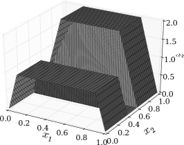
Figure 1: Target function $\hat{z}$ for the control examples.

A spatial finite element mesh of piecewise linear triangular elements is used. The mesh is constructed as $2^{7}\times 2^{7}$ squares and each square is subdivided into two triangular finite element cells. This yields $N=16\,441$ spatial degrees of freedom. The stochastic Galerkin discretisation is based on seven-dimensional Legendre polynomials of order two. This yields $Q=36$ (when $u^{\prime}=0$ in (10)) and the algebraic system in (45) has dimension $1.2\cdot 10^{6}\times 1.2\cdot 10^{6}$. The stochastic collocation method employs a level-two Smolyak sparse grid based on Gauss–Legendre collocation points with $Q=141$ collocation points.

The computer code used for the examples is built on the library DOLFIN [15]. The complete computer code for all presented examples is available as part of the supporting material [20].

Distributive control with cost functional $\mathcal{J}_{1}$

First, we consider a distributive control via $u$ only and using the cost functional $\mathcal{J}_{1}$ in (7) with $\delta=0$. A control function $u$ with the additive structure in (10) is used. The goal is to determine an optimal mean control $\bar{u}$, which is the deterministic input for the controller response.

Perfect controller case

The optimal control for the case $u^{\prime}=0$, which corresponds to the controller action being wholly deterministic, and $\beta=0$, which implies no extra control over the variance of $z$, is computed and the results are shown in Fig. 2 for the case $\gamma=10^{-5}$. The computed mean of the state function, the variance of the state function and the control $\bar{u}$ are all shown. The same quantities are presented in Fig. 3 for the case $\gamma=10^{-3}$. Comparing the results in Figs. 2 and 3, as expected the larger $\gamma$-penalty term leads to a poorer approximation of the target. The values of the cost functional, tracking error $\mathinner{\!\left\lVert z-\hat{z}\right\rVert}^{2}_{L^{2}(D)\otimes L^{2}_{\rho}(\Gamma)}$ and standard deviation $\mathinner{\!\left\lVert\mathrm{std}(z)\right\rVert}_{L^{2}(D)}^{2}$ are summarised in Table 1. The tracking error as a function of $\gamma$ is presented in Fig. 4, illustrating the deterioration in the quality of the computed result for increasing values of $\gamma$.

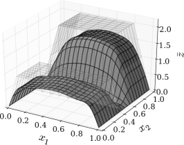
(a) mean state

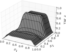
(b) variance state

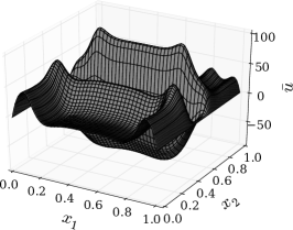
(c) deterministic control

Figure 2: Mean and variance of the optimal state and deterministic control variable $u=\bar{u}$ ($u^{\prime}=0$) associated with the cost functional $\mathcal{J}_{1}$ and computed with the stochastic Galerkin method with $\alpha=1$, $\beta=\delta=0$ and $\gamma=10^{-5}$. The target $\hat{z}$ is illustrated transparently in (a) for reference.

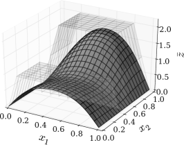
(a) mean state

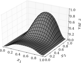
(b) variance state

(c) deterministic control

Figure 3: Mean and variance of the optimal state and deterministic control variable $u=\bar{u}$ ($u^{\prime}=0$) associated with the cost functional $\mathcal{J}_{1}$ and computed with the stochastic Galerkin method with $\alpha=1$, $\beta=\delta=0$ and $\gamma=10^{-3}$. The target $\hat{z}$ is illustrated transparently in (a) for reference.

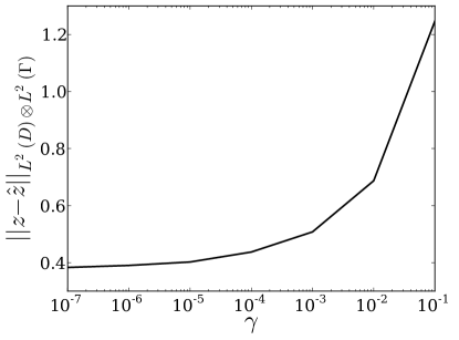
Figure 4: Tracking error $\mathinner{\!\left\lVert z-\hat{z}\right\rVert}_{L^{2}(D)\otimes L^{2}_{\rho}(\Gamma)}$ as a function of the penalty parameter $\gamma$ for the problem considered in Section 6.1.1.

Imperfect controller case

We now consider the impact of an imperfect controller by introducing a known non-zero stochastic term $u^{\prime}$. The stochastic function $u^{\prime}$ is modelled by a three-term Karhunen–Loève expansion based on a zero-mean Gaussian field with an exponential covariance function, unit variance and a unit correlation length. For the examples in this section we set $\gamma=10^{-3}$.

The computed mean and second central moment of the state $z$ and the computed mean optimal control $\bar{u}$ are depicted in Fig. 5 for the case $\beta=0$, and in Fig. 6 for the case $\beta=1$. A comparison between Fig. 2, which corresponds to the case $u^{\prime}=0$, and Fig. 5 shows that the prescribed uncertainty on the control has only a limited effect on the outcome of the optimal control problem for this example. The mean control $\bar{u}$ is visibly unchanged and the variance of the state variable increases slightly. This observation is also reflected in the computed values for the cost functional (see Table 1).

(a) mean state

(b) variance state

(c) mean control

Figure 5: Mean and variance of the optimal state and mean control variable $\bar{u}$ ($u^{\prime}\neq 0$) associated with the cost functional $\mathcal{J}_{1}$ and computed with the stochastic Galerkin method with $\alpha=1$, $\beta=\delta=0$ and $\gamma=10^{-3}$. The target $\hat{z}$ is illustrated transparently in (a) for reference.

To provide control over the variance of the state variable, the parameter $\beta$ in the cost functional (20) can be increased. Comparing the results in Fig. 5 ($\beta=0$) and Fig. 6 ($\beta=1$), the peak variance is reduced, but the correspondence between the mean state and the target is compromised.

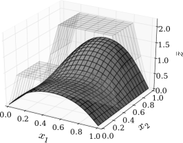
(a) mean state

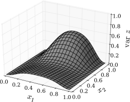
(b) variance state

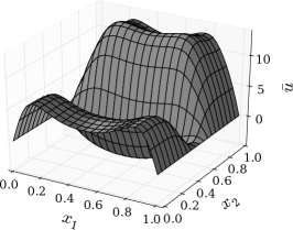
(c) mean control

Figure 6: Mean and variance of the optimal state and mean control variable $\bar{u}$ ($u^{\prime}\neq 0$) associated with the cost functional $\mathcal{J}_{1}$ and computed with the stochastic Galerkin method with $\alpha=1$, $\beta=1$, $\delta=0$ and $\gamma=10^{-3}$. The target $\hat{z}$ is illustrated transparently in (a) for reference.

Distributive control with cost functional $\mathcal{J}_{2}$

We now mirror the imperfect controller problem considered in Section 6.1.2, but for the cost functional $\mathcal{J}_{2}$. The cost functional $\mathcal{J}_{1}$ provides a measure of the average distance between the state and target, whereas the cost functional $\mathcal{J}_{2}$ provides a measure of the distance between the mean state and the target.

For the examples we adopt $\alpha=1$, $\gamma=10^{-3}$ and $\delta=0$ in $\mathcal{J}_{2}$. For the case $\beta=0$, which implies no extra control over the variance of the response, the mean and the variance of the computed state variable $z$ and the computed deterministic part of the control signal $\bar{u}$ are shown in Fig. 7. Compared to the case presented in Fig. 5, the mean of the computed state variable is a better approximation of the target, while the variance of the state variable is significantly larger. A similar result was observed for the case $u^{\prime}=0$. Fig. 8 shows the computed results for the case $\beta=1$. Increasing $\beta$ reduces the variance of the response, but comes at the expense of the approximation of the target by the mean state.

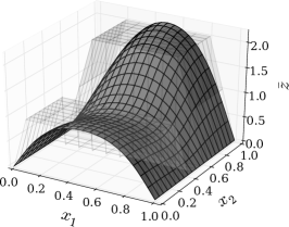
(a) mean state

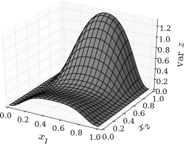
(b) variance state

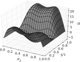
(c) mean control

Figure 7: Mean and variance of the optimal state and mean control variable $\bar{u}$ ($u^{\prime}\neq 0$) associated with the cost functional $\mathcal{J}_{2}$ and computed with the stochastic Galerkin method with $\alpha=1$, $\beta=\delta=0$ and $\gamma=10^{-3}$. The target $\hat{z}$ is illustrated transparently in (a) for reference.

(a) mean state

(b) variance state

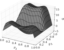
(c) mean control

Figure 8: Mean and variance of the optimal state and mean control variable $\bar{u}$ ($u^{\prime}\neq 0$) associated with the cost functional $\mathcal{J}_{2}$ and computed with the stochastic Galerkin method with $\alpha=1$, $\beta=1$, $\delta=0$ and $\gamma=10^{-3}$. The target $\hat{z}$ is illustrated transparently in (a) for reference.

The advantage of using the cost functional $\mathcal{J}_{2}$ over $\mathcal{J}_{1}$ is that it permits a greater tuning of the relative importance of the mean response versus the variance of the response, via the parameters $\alpha$ and $\beta$. In the case of the cost functional $\mathcal{J}_{1}$, the variance of the state variable is already implicitly minimised by the $\alpha$ term as it is a norm over $L^{2}(D)\times L^{2}_{\rho}(\Omega)$. For the $\mathcal{J}_{1}$ case, increasing $\beta$ only entails an additional contribution of the variance to the cost functional.

	$\mathcal{J}(z,u)$	$\mathinner{\!\left\lVert z-\hat{z}\right\rVert}^{2}_{L^{2}(D)\otimes L^{2}_{\rho}(\Gamma)}$	$\>\mathinner{\!\left\lVert\mathrm{std}(z)\right\rVert}_{L^{2}(D)}^{2}$
deterministic control $u=\bar{u}(x)$, $u^{\prime}(x,y)=0$
cost functional $\mathcal{J}_{1}$, $\beta=0$, $\gamma=10^{-5}$	$2.083\times 10^{-1}$	$4.022\times 10^{-1}$	$2.562\times 10^{-1}$
cost functional $\mathcal{J}_{1}$, $\beta=0$, $\gamma=10^{-3}$	$2.911\times 10^{-1}$	$5.078\times 10^{-1}$	$1.845\times 10^{-1}$
unknown mean control $\bar{u}(x)$, var($u^{\prime}$)$=1$
cost functional $\mathcal{J}_{1}$, $\beta=0$, $\gamma=10^{-3}$	$2.956\times 10^{-1}$	$5.160\times 10^{-1}$	$1.927\times 10^{-1}$
cost functional $\mathcal{J}_{1}$, $\beta=1$, $\gamma=10^{-3}$	$3.767\times 10^{-1}$	$5.636\times 10^{-1}$	$1.367\times 10^{-1}$
cost functional $\mathcal{J}_{2}$, $\beta=0$, $\gamma=10^{-3}$	$1.764\times 10^{-1}$	$2.353\times 10^{-1}$	$2.957\times 10^{-1}$
cost functional $\mathcal{J}_{2}$, $\beta=1$, $\gamma=10^{-3}$	$2.956\times 10^{-1}$	$3.233\times 10^{-1}$	$1.927\times 10^{-1}$

Table 1: Summary of the cost functional, tracking error and standard deviation of the state variable for the considered optimal control problems with a distributive control function.

Boundary control with cost functional $\mathcal{J}_{1}$

In practical applications it is often more plausible to control boundary values rather than the source term. In this section, we consider the same model problem as in Section 6.1, but now an optimal boundary flux control is computed (now $\gamma=0$ in the cost functionals). The right-hand side function in the constraint equation (4) is set to $u=5$. The control boundary flux is computed on the ‘upper’ ($x_{2}=1$) and ‘lower’ ($x_{2}=0$) boundaries.

Perfect controller case

Fig. 9 presents the computed mean state, variance of the state and the boundary flux control $\bar{g}$ for the parameters $\alpha=1$, $\beta=\gamma=0$ and $\delta=10^{-3}$, and with $g^{\prime}=0$. The corresponding values of the cost functional and tracking errors are given in Table 2. As can be anticipated, correspondence between the optimal state and target is poorer in the case of a boundary control than in the case of a distributive control (see Fig. 3). The variance of the state variable in Fig. 9 can be countered by increasing the parameter $\beta$. Results for the case $\beta=1$ are presented in Fig. 10. The reduction in the variance is accompanied by a deterioration in the approximation of the target function.

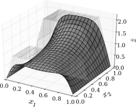
(a) mean state

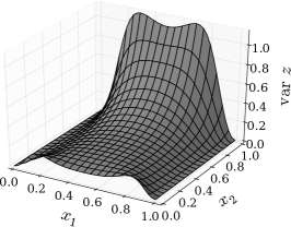
(b) variance state

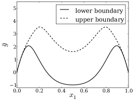
(c) deterministic control

Figure 9: Mean and variance of the optimal state and deterministic control variable $g=\bar{g}$ ($g^{\prime}=0$) associated with the cost functional $\mathcal{J}_{1}$ and computed with the stochastic Galerkin method with $\alpha=1$, $\gamma=0$, $\delta=10^{-3}$ and $\beta=0$. The target $\hat{z}$ is illustrated transparently in (a) for reference.

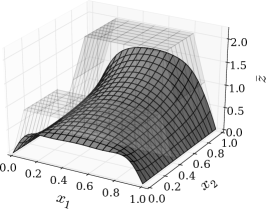
(a) mean state

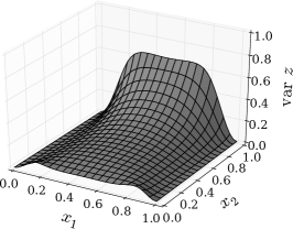
(b) variance state

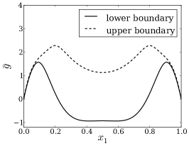
(c) deterministic control

Figure 10: Mean and variance of the optimal state and deterministic control variable $g=\bar{g}$ ($g^{\prime}=0$) associated with the cost functional $\mathcal{J}_{1}$ and computed with the stochastic Galerkin method with $\alpha=1$, $\gamma=0$, $\delta=10^{-3}$ and $\beta=1$. The target $\hat{z}$ is illustrated transparently in (a) for reference.

Imperfect controller case

We now consider the impact of an imperfect controller by decomposing the boundary control $g$ according to (10). The zero-mean stochastic function $g^{\prime}$ is modelled by a three-term Karhunen–Loève expansion based on a Gaussian field with an exponential covariance function, a variance of $0.25$ and unit correlation length.

Fig. 11 presents the optimal mean boundary control $\bar{g}$ along with the first moments of the state variable. The values of the cost functional and tracking errors are given in Table 2. The mean optimal control $\bar{g}$ and the mean state appear visibly equal to the results in Fig. 9 for the case where a perfect control device, i.e., with $g^{\prime}=0$, is modelled, while the variance of $z$ is slightly larger.

(a) mean state

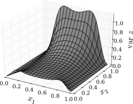
(b) variance state

(c) mean control

Figure 11: Mean and variance of the optimal state and mean control variable $\bar{g}$ ($g^{\prime}\neq 0$) associated with the cost functional $\mathcal{J}_{1}$ and computed with the stochastic Galerkin method with $\alpha=1$, $\beta=\gamma=0$ and $\delta=10^{-3}$. The target $\hat{z}$ is illustrated transparently in (a) for reference.

	$\mathcal{J}(z,g)$	$\mathinner{\!\left\lVert z-\hat{z}\right\rVert}^{2}_{L^{2}(D)\otimes L^{2}_{\rho}(\Gamma)}$	$\>\mathinner{\!\left\lVert\mathrm{std}(z)\right\rVert}_{L^{2}(D)}^{2}$
deterministic control $g=\bar{g}(x)$, $g^{\prime}(x,y)=0$
cost functional $\mathcal{J}_{1}$, $\beta=0$, $\delta=10^{-3}$	$2.711\times 10^{-1}$	$5.421\times 10^{-1}$	$2.091\times 10^{-1}$
cost functional $\mathcal{J}_{1}$, $\beta=1$, $\delta=10^{-3}$	$3.593\times 10^{-1}$	$5.757\times 10^{-1}$	$1.428\times 10^{-1}$
unknown mean control $\bar{g}(x)$, var($g^{\prime}$)$=0.25$
cost functional $\mathcal{J}_{1}$, $\beta=0$, $\delta=10^{-3}$	$2.753\times 10^{-1}$	$5.499\times 10^{-1}$	$2.168\times 10^{-1}$
cost functional $\mathcal{J}_{1}$, $\beta=1$, $\delta=10^{-3}$	$3.673\times 10^{-1}$	$5.835\times 10^{-1}$	$1.506\times 10^{-1}$

Table 2: Summary of the cost functional, tracking error and standard deviation of the state variable for the considered optimal control problems with a boundary control function.

Stochastic inverse examples

When the additive structure of the control function is not enforced and $u$ is permitted to be stochastic and unknown, the optimal control problem effectively becomes a stochastic inverse problem. In this case, the stochastic properties of $u$ are unknown, but will be computed. The problem is: given an observation $\hat{z}$ of a system that must obey the constraints in (4)–(6), find the stochastic source term $u$ that would induce the response $\hat{z}$. Computed higher moments of $u$ provide information on the uncertainty of the driving term. This formulation of the problem is not useful for control problems, since the properties of a control device are considered to be known and it is unclear how a stochastic $u$ could be used as a control signal. The mean of $u$ could be taken as the control, but this will not in general be the optimal control and computing the uncertainty in the system response would require an additional computation.

Stochastic inverse problems associated with the cost functional $\mathcal{J}_{1}$ or $\mathcal{J}_{2}$ and the constraint equations (17)–(19) are solved using the same computational domain, boundary conditions, representation of $\kappa$ and discretisation parameters as in Section 6. For inverse problems, the collocation systems remain decoupled for $\beta=0$ in the cost functional $\mathcal{J}_{1}$. We present some simple examples using a target function $\hat{z}$ that is computed by solving the stochastic forward problem in (17)–(19) with the deterministic source function

$$\hat{u}\mathrel{\mathop{\mathchar 58\relax}}=50\sin(\pi x_{1})\cos(2\pi x_{2}).$$ (69)

Figure 12 illustrates $\hat{u}$ and the first moments of the target function that will be used. We aim to illustrate how the presented framework can be used for a class of inverse problems. Application to realistic inverse problems will require deeper investigations into handling noisy and incomplete data.

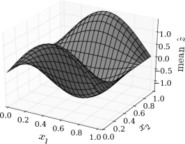
(a) mean target

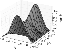
(b) variance target

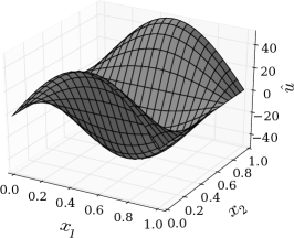
(c) deterministic source

Figure 12: (a)–(b) Mean and variance of the target function $\hat{z}$ for solving a stochastic inverse problem. (c) Deterministic source $\hat{u}$ used for constructing $\hat{z}$ as the solution of the forward problem.

Determination of the source function using cost functional $\mathcal{J}_{1}$

We consider the case with $\beta=0$, which permits the decoupled solution of problems at collocation points. We therefore apply both the stochastic Galerkin and collocation methods in this section.

Deterministic target

As a first case, we consider a stochastic inverse problem with the cost functional $\mathcal{J}_{1}$ and with the target $\hat{z}$ taken as the mean of the forward problem. This represents an inverse problem where only one observation of the system response is available; some stochastic data computed in the forward problem has been discarded. Recall that the stochastic properties of $\kappa$ are known.

The computed first moments of the state and source function, using $\alpha=1$, $\beta=\delta=0$ and $\gamma=10^{-5}$, are shown in Fig. 13. The computed cost functional and tracking error are presented in Table 3. The mean of the target $\hat{z}$ and the mean of the state variable $\bar{z}$ coincide visually, whereas there is a considerable difference between the actual source $\hat{u}$ and the mean of the computed source $\bar{u}$. A large variance of the computed source term relative to its mean is also observed. This is inherent to the posed problem as limited observation data is being used. As $\gamma$ approaches zero, the tracking error is observed to approach zero, as shown in Fig. 14. This figure contrasts the tracking error in Fig. 4 for a control problem, in which case the considered target cannot be reached as the target is not a solution of the forward problem.

(a) mean state

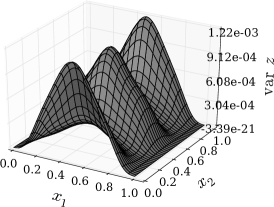
(b) variance state

(c) mean source

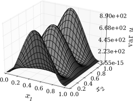
(d) variance source

Figure 13: Mean and variance of the state and source variable for an inverse problem associated with the cost functional $\mathcal{J}_{1}$ and computed with the stochastic collocation method with $\alpha=1$, $\beta=\delta=0$ and $\gamma=10^{-5}$. The mean of the solution to the forward problem is used as the target. The deterministic source $\hat{u}$ is illustrated transparently in (c) for reference.

Figure 14: Tracking error $\mathinner{\!\left\lVert z-\hat{z}\right\rVert}_{L^{2}(D)\otimes L^{2}_{\rho}(\Gamma)}$ as a function of the penalty parameter $\gamma$ for the inverse problem considered in Section 7.1.1.

Stochastic target

A stochastic target in now considered, which is the complete solution of the forward problem. Hence, no data has been discarded from the forward problem. The computed mean of the state variable, the variance of the state variable, the mean of the computed source and the variance of the source function are shown in Fig. 15 for the case $\alpha=1$, $\beta=0$, $\delta=0$ and $\gamma=10^{-5}$. The results were computed using the collocation method. The statistics of the state variable and the target visually coincide. A measure of the quality of the approximation is quantified by the tracking error in Table 3. As the penalty parameter $\gamma$ is decreased the computed state variable better matches the stochastic target. This effect is illustrated in Fig. 16, for which $\gamma=10^{-8}$, and in Table 3. The computed source term in Fig. 16 matches the exact solution $\hat{u}$ very well in both the mean and the variance (which is zero for $\hat{u}$). The stochastic Galerkin method yields similar results, as indicated in Table 3 where various quantities computed with the two methods are summarised.

(a) mean state

(b) variance state

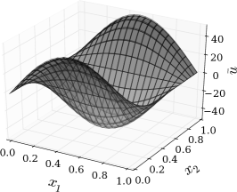
(c) mean source

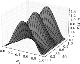
(d) variance source

Figure 15: Mean and variance of the state and source variable for an inverse problem associated with the cost functional $\mathcal{J}_{1}$ and computed with the stochastic collocation method with $\alpha=1$, $\beta=\delta=0$ and $\gamma=10^{-5}$. The mean and variance of the target $\hat{z}$ are illustrated in Fig. 12. The deterministic source $\hat{u}$ is illustrated transparently in (c) for reference.

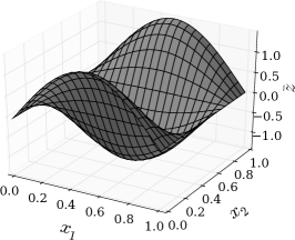
(a) mean state

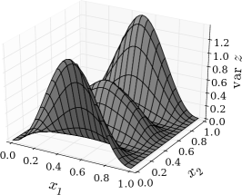
(b) variance state

(c) mean source

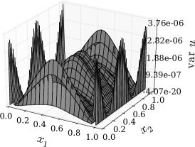
(d) variance source

Figure 16: Mean and variance of the state and source variable for an inverse problem associated with the cost functional $\mathcal{J}_{1}$ and computed with the stochastic collocation method with $\alpha=1$, $\beta=\delta=0$ and $\gamma=10^{-8}$. The mean and variance of the target $\hat{z}$ are illustrated in Fig. 12. The deterministic source $\hat{u}$ is illustrated transparently in (c) for reference.

For small penalty parameters, limited control over the source function is imposed, which can lead to a more expensive iterative solution of the one-shot systems. In the stochastic Galerkin case, the convergence rate of the mean-based preconditioner (see Section 5.1) deteriorates severely for small values of $\gamma$. The collective multigrid method shows robust convergence behaviour. A similar observation on the computational complexity was made by Zabaras [27]. Also, observe the non-smooth variance of the source function on the domain boundaries for $\gamma=10^{-8}$ in Fig. 16(d).

Determination of the source function using cost functional $\mathcal{J}_{2}$

We mirror the stochastic inverse problem considered in Section 7.1.1, but now for the cost functional $\mathcal{J}_{2}$. The $\mathcal{J}_{2}$ formulation involves the mean of an unknown field, which means that a stochastic collocation formulation will not lead to decoupled problems when $\alpha\neq 0$. Fig. 17 shows the computed mean and variance of the state and source functions, computed with the stochastic Galerkin method. As in Fig. 13, the mean of the state variable and the mean target visually coincide. Since the variance of the state variable does not contribute to $\mathcal{J}_{2}$, a larger variance is observed than in Fig. 13(b). The computed source function clearly differs (note the magnitudes) from that computed when using the cost functional $\mathcal{J}_{1}$. The corresponding values of the cost functional and tracking error are summarised in Table 3.

(a) mean state

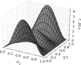
(b) variance state

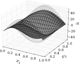
(c) mean source

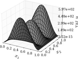
(d) variance source

Figure 17: Mean and variance of the state and source variable for an inverse problem associated with the cost functional $\mathcal{J}_{2}$ and computed with the stochastic collocation method with $\alpha=1$, $\beta=\delta=0$ and $\gamma=10^{-5}$. The mean and variance of the target $\hat{z}$ are illustrated in Fig. 12. The deterministic source $\hat{u}$ is illustrated transparently in (c) for reference.

	$\mathcal{J}(z,u)$	$\mathinner{\!\left\lVert z-\hat{z}\right\rVert}^{2}_{L^{2}(D)\otimes L^{2}_{\rho}(\Gamma)}$		$e_{u}$
Stochastic Galerkin finite element solution ($Q=36$)
cost functional $\mathcal{J}_{1}$, $\hat{z}$ deterministic, $\gamma=10^{-5}$	$6.786\times 10^{-3}$	$7.225$$\ \times\$	$10^{-4}$	4.368$\ \times\$	$10^{-1}$
cost functional $\mathcal{J}_{1}$, $\hat{z}$ stochastic, $\gamma=10^{-5}$	$3.035\times 10^{-3}$	$1.678$$\ \times\$	$10^{-4}$	1.505$\ \times\$	$10^{-3}$
cost functional $\mathcal{J}_{1}$, $\hat{z}$ stochastic, $\gamma=10^{-8}$	$3.123\times 10^{-6}$	$1.882$$\ \times\$	$10^{-10}$	2.339$\ \times\$	$10^{-9}$
cost functional $\mathcal{J}_{2}$, $\gamma=10^{-5}$	$2.107\times 10^{-3}$	$3.784$$\ \times\$	$10^{-5}$	3.193$\ \times\$	$10^{-1}$
cost functional $\mathcal{J}_{2}$, $\gamma=10^{-8}$	$2.127\times 10^{-6}$	$9.833$$\ \times\$	$10^{-11}$	3.190$\ \times\$	$10^{-1}$
Stochastic collocation finite element solution ($Q=141$)
cost functional $\mathcal{J}_{1}$, $\hat{z}$ deterministic, $\gamma=10^{-5}$	$6.957\times 10^{-3}$	$7.406$$\ \times\$	$10^{-4}$	$4.556$$\ \times\$	$10^{-1}$
cost functional $\mathcal{J}_{1}$, $\hat{z}$ stochastic, $\gamma=10^{-5}$	$3.035\times 10^{-3}$	$1.678$$\ \times\$	$10^{-4}$	$1.506$$\ \times\$	$10^{-3}$
cost functional $\mathcal{J}_{1}$, $\hat{z}$ stochastic, $\gamma=10^{-8}$	$3.123\times 10^{-6}$	$1.882$$\ \times\$	$10^{-10}$	$2.334$$\ \times\$	$10^{-9}$

Table 3: Summary of the cost functional, tracking error of the state variable and relative error $e_{u}\mathrel{\mathop{\mathchar 58\relax}}=\mathinner{\!\left\lVert u-\hat{u}\right\rVert}^{2}_{L^{2}(D)\otimes L^{2}_{\rho}(\Gamma)}/\mathinner{\!\left\lVert\hat{u}\right\rVert}^{2}_{L^{2}(D)}$ of the computed source for the considered inverse problems with unknown source function.

Conclusions

A one-shot solution approach for stochastic optimal control problems with PDE constraints has been presented. The problem was formulated as an optimisation problem constrained by a stochastic elliptic PDE, and the framework is sufficiently general to also address a class of inverse problems that involve uncertainty. Statistical moments have been included in the cost functional and uncertainty in the controller response has been accounted for. To compute solutions, a one-shot method is combined with stochastic finite element discretisations. It is shown that the non-intrusivity property of the stochastic collocation method is lost when moments of the state variable appear in the cost functional, or when the control function is a deterministic function. We argue that the control function must contain a deterministic component in order for the problem to constitute a control problem, versus a stochastic inverse problem, hence the non-intrusivity property of the stochastic collocation method will be lost for one-shot formulations. Applying a stochastic Galerkin method does not impose additional difficulties compared to solving stochastic PDEs, hence, for the method presented in this work the stochastic Galerkin method is preferred over the collocation method for control problems. In the case of inverse problems, where the function to be found is wholly stochastic, it was shown that it is possible in some cases to preserve the non-intrusivity property of the stochastic collocation method.

The formulated methods are supported by extensive numerical experiments that address both optimal control and inverse problems. The computed results illustrate the impact of various options in the formulation and the difference between the considered cost functionals. In particular, examples show the impact, for the considered model problem, of the different ways in which statistical data can be included in the cost functionals.

Acknowledgement

This work was performed while E. Rosseel was a visiting researcher at the University of Cambridge with support from the Research Foundation Flanders (Belgium).

Appendix A Evaluating derivatives of stochastic functions

Analytical expressions for inner products of the form

$$\int_{\Gamma}\nabla_{y}\psi_{i}(y)\cdot\nabla_{y}\psi_{j}(y)\rho\operatorname{d\!}y$$ (70)

are derived here based on the orthogonality properties of the generalised polynomial chaos basis functions $\psi_{i}$ in (37). Given (37) and $\delta$ the Kronecker delta, the integral (70) can be rewritten as

$$\int_{\Gamma}\nabla_{y}\psi_{i}(y)\cdot\nabla_{y}\psi_{j}(y)\rho\operatorname{d\!}y=\sum_{k=1}^{L}\prod_{t=1,t\neq k}^{L}\delta_{i_{t},j_{t}}\int_{\Gamma_{k}}\frac{d\varphi_{i_{k}}}{dy_{k}}\frac{d\varphi_{j_{k}}}{dy_{k}}\rho\operatorname{d\!}y_{k}.$$ (71)

Hermite polynomials.

In the case of Hermite polynomials, which are normalised with respect to a standard normal distribution, the derivative of $\varphi_{i_{k}}$ is given by

$$\frac{d\varphi_{i_{k}}}{dy_{k}}=\sqrt{i_{k}}\varphi_{i_{k}-1}.$$ (72)

Expression (71) then simplifies to

$$\int_{\Gamma}\nabla_{y}\psi_{i}(y)\cdot\nabla_{y}\psi_{j}(y)\rho\operatorname{d\!}y=\delta_{i,j}\sum_{k=1}^{L}j_{k}.$$ (73)

Legendre polynomials.

In the case of Legendre polynomials, normalised and scaled to a uniform distribution on $\mathinner{\left[-\sqrt{3},\sqrt{3}\right]}$, it can be shown that the following relation holds:

$$\frac{d\varphi_{i_{k}}}{dy_{k}}=\frac{\sqrt{3\mathinner{\left(2i_{k}+1\right)}}}{3}\sum_{t=0}^{\left\lfloor\frac{j_{k}-1}{2}\right\rfloor}\sqrt{2\mathinner{\left(i_{k}-1-2t\right)}+1}\varphi_{i_{k}-1-2t}.$$ (74)

After some calculations, expression (71) corresponds to

$$\int_{\Gamma}\nabla_{y}\psi_{i}(y)\cdot\nabla_{y}\psi_{j}(y)\rho\operatorname{d\!}y=\sum_{k=1}^{L}\mathinner{\left(1-\mathinner{\left(\mathinner{\left(i_{k}+j_{k}\right)}\bmod 2\right)}\right)}\frac{\sqrt{2i_{k}+1}\sqrt{2j_{k}+1}}{3}\\ \left\lfloor\frac{\min\mathinner{\left(i_{k},j_{k}\right)}+1}{2}\right\rfloor\mathinner{\left(1-2\left\lfloor\frac{1-\min\mathinner{\left(i_{k},j_{k}\right)}}{2}\right\rfloor\right)}\prod_{t=1,t\neq k}^{L}\delta_{j_{t},i_{t}}.$$ (75)

References

- Babuška et al. [2004] I. Babuška, R. Tempone, and G. Zouraris. Galerkin finite element approximations of stochastic elliptic partial differential equations. SIAM J. Numer. Anal., 42:800–825, 2004.
- Babuška et al. [2007] I. Babuška, F. Nobile, and R. Tempone. A stochastic collocation method for elliptic partial differential equations with random input data. SIAM J. Numer. Anal., 45:1005–1034, 2007.
- Babuška et al. [2010] I. Babuška, F. Nobile, and R. Tempone. A stochastic collocation method for elliptic partial differential equations with random input data. SIAM Rev., 52(2):317–355, 2010.
- Bäck et al. [2011] J. Bäck, F. Nobile, L. Tamellini, and R. Tempone. Stochastic spectral Galerkin and collocation methods for PDEs with random coefficients: A numerical comparison. In J. S. Hesthaven and E. M. Rønquist, editors, Spectral and High Order Methods for Partial Differential Equations, volume 76 of Lecture Notes in Computational Science and Engineering, pages 43–62. Springer Berlin Heidelberg, 2011.
- Borzì [2010] A. Borzì. Multigrid and sparse-grid schemes for elliptic control problems with random coefficients. Comput. Visual Sci., 13(4):153–160, 2010.
- Borzì and Schulz [2009] A. Borzì and V. Schulz. Multigrid methods for PDE optimization. SIAM Rev., 51(2):361–395, 2009.
- Borzì and von Winckel [2009] A. Borzì and G. von Winckel. Multigrid methods and sparse-grid collocation techniques for parabolic optimal control problems with random coefficients. SIAM J. Sci. Comput., 31(3):2172–2192, 2009.
- Frauenfelder et al. [2005] P. Frauenfelder, C. Schwab, and R. A. Todor. Finite elements for elliptic problems with stochastic coefficients. Comput. Methods Appl. Mech. Engrg., 194:205–228, 2005.
- Ghanem and Spanos [2003] R. G. Ghanem and P. D. Spanos. Stochastic Finite Elements: A Spectral Approach. Dover, Mineola, New York, USA, 2nd edition, 2003.
- Gunzburger [2003] M. D. Gunzburger. Perspectives in Flow Control and Optimization. SIAM, Philadelphia, USA, 2003.
- Hinze et al. [2009] M. Hinze, R. Pinnau, M. Ulbrich, and S. Ulbrich. Optimization with PDE Constraints. Springer, Berlin, Germany, 2009.
- Hou et al. [2011] L. S. Hou, J. Lee, and H. Manouzi. Finite element approximations of stochastic optimal control problems constrained by stochastic elliptic PDEs. J. Math. Anal. Appl., 384(1):87–103, 2011.
- Jin and Zou [2008] B. Jin and J. Zou. Inversion of Robin coefficient by a spectral stochastic finite element approach. J. Comput. Phys., 227:3282–3306, 2008.
- Loève [1977] M. Loève. Probability Theory. Springer, New York, USA, 1977.
- Logg and Wells [2010] A. Logg and G. N. Wells. DOLFIN: Automated finite element computing. ACM Trans Math Software, 37(2):20:1–20:28, 2010.
- Matthies and Keese [2005] H. G. Matthies and A. Keese. Galerkin methods for linear and nonlinear elliptic stochastic partial differential equations. Comput. Methods Appl. Mech. Engrg., 194:1295–1331, 2005.
- Powell and Elman [2009] C. E. Powell and H. C. Elman. Block-diagonal preconditioning for spectral stochastic finite element systems. IMA J. Numer Anal., 29:350–375, 2009.
- Rees et al. [2010] T. Rees, H. S. Dollar, and A. J. Wathen. Optimal solvers for PDE-constrained optimization. SIAM J. Sci. Comput., 32:271–298, 2010.
- Rosseel and Vandewalle [2010] E. Rosseel and S. Vandewalle. Iterative solvers for the stochastic finite element method. SIAM J. Sci. Comput., 32(1):372–397, 2010.
- Rosseel and Wells [2011] E. Rosseel and G. N. Wells. Supporting material, 2011. URL http://www.eng.cam.ac.uk/~gnw20/stochastic_control.tar.gz.
- Sankaran [2009] S. Sankaran. Stochastic optimization using a sparse grid collocation scheme. Prob. Eng. Mech., 24:382–396, 2009.
- Schöberl and Zulehner [2007] J. Schöberl and W. Zulehner. Symmetric indefinite preconditioners for saddle point problems with applications to PDE-constrained optimization problems. SIAM J. Math. Anal., 29(3):752–773, 2007.
- Tröltzsch [2010] F. Tröltzsch. Optimal Control of Partial Differential Equations: Theory, Methods and Applications. American Mathematical Society, Providence, Rhode Island, USA, 2010.
- Xiu [2009] D. Xiu. Fast numerical methods for stochastic computations: A review. Commun. Comput. Phys., 5(2–4):242–272, 2009.
- Xiu and Hesthaven [2005] D. Xiu and J. S. Hesthaven. High-order collocation methods for differential equations with random inputs. SIAM J. Sci. Comput., 27(3):1118–1139, 2005.
- Xiu and Karniadakis [2002] D. Xiu and G. E. Karniadakis. Modeling uncertainty in steady state diffusion problems via generalized polynomial chaos. Comput. Methods Appl. Mech. Engrg., 191:4927–4948, 2002.
- Zabaras [2011] N. Zabaras. Solving stochastic inverse problems: a sparse grid collocation approach. In L. Biegler, G. Biros, O. Ghattas, Y. Marzouk, M. Heinkenschloss, D. Keyes, B. Mallick, L. Tenorio, B. van Bloemen Waanders, and K. Willcox, editors, Large-scale Inverse Problems and Quantification of Uncertainty, chapter 14, pages 291–319. Wiley, 2011.
- Zabaras and Ganapathysubramanian [2008] N. Zabaras and B. Ganapathysubramanian. A scalable framework for the solution of stochastic inverse problems using a sparse grid collocation approach. J. Comput. Phys., 227:4697–4735, 2008.