Causality and quantum interference in time-delayed laser-induced nonsequential double ionization

Abstract

We perform a detailed analysis of the importance of causality within the strong-field approximation and the steepest descent framework for the recollision-excitation with subsequent tunneling ionization (RESI) pathway in laser-induced nonsequential double ionization (NSDI). In this time-delayed pathway, an electron returns to its parent ion, and, by recolliding with the core, gives part of its kinetic energy to excite a second electron at a time $t^{\prime}$. The second electron then reaches the continuum at a later time $t$ by tunneling ionization. We show that, if $t^{\prime}$ and $t$ are complex, the condition that recollision of the first electron occurs before tunnel ionization of the second electron translates into boundary conditions for the steepest-descent contours, and thus puts constraints on the saddles to be taken when computing the RESI transition amplitudes. We also show that this generalized causality condition has a dramatic effect in the shapes of the RESI electron momentum distributions for few-cycle laser pulses. Physically, causality determines how the dominant sets of orbits an electron returning to its parent ion can be combined with the dominant orbits of a second electron tunneling from an excited state. All features encountered are analyzed in terms of such orbits, and their quantum interference.

I Introduction

Phenomena occurring in the interaction of matter with intense, low-frequency laser fields, such as high-order harmonic generation (HHG), above-threshold ionization (ATI), and laser-induced nonsequential double ionization (NSDI), owe their existence to laser-induced recombination or rescattering processes, in which a previously released electron interacts with its parent ion Corkum . The identification of their common dynamical origin has been instrumental to exploit these effects in a number of applications, such as for the generation of attosecond pulses atto1996 and the dynamic imaging of matter with subfemtosecond precision Attoreview . Since this mechanism is intimately linked to specific dynamical pathways, it also led to efficient semi-analytical approaches, such as the strong-field approximation (SFA) (for seminal work on ionization and laser induced rescattering see, e.g., SFA and SFAresc , respectively). In this approach, the quantum-mechanical transition amplitude is associated to the orbits of an electron returning to its parent ion. The transition amplitude corresponding to a particular strong-field process takes the form of a multiple integral, which, in many cases, can be solved employing saddle-point methods SFApath .

It is also a well-known fact that the orbits along which the active electron returns typically occur in pairs. In particular, thresholds can often be associated to conditions where the two orbits of a given pair become almost degenerate. This violates the saddle-point assumption which leads to expressions in terms of individual orbits, but can be treated successfully in a uniform approximation which describes the two orbits collectively schomerussieber . This approximation has been first applied in strong-field physics to ATI Uniform2002 and, since then, has been used in a wide range of phenomena, such as HHG HHGuniform and NSDI NSDI2004_1 ; NSDI2004_2 ; NSDI2005 . This latter phenomenon is a typical example of a highly correlated two-electron process occurring in strong laser fields. The physical mechanism behind it is a three-step process in which the first electron is released in the continuum by tunneling or multiphoton ionization, and gains kinetic energy from the field. Subsequently, it is driven back by the field towards its parent ion, with which it rescatters. In this recollision, part of its kinetic energy is transferred to the core, so that a second electron is freed.

There are several pathways through which NSDI may occur. Both electrons may, for instance, be released simultaneously in a scattering process in which the first electron, upon return, provides the second electron with enough energy for it to overcome the second ionization potential. This process is known as electron-impact ionization. This pathway has been successfully used to explain a number of experimentally observed features in the electron momentum distribution, such as peaks at non-vanishing momenta VShape1 ; VShape2 ; NSDI2005 , and the recently observed V-shaped structure which can been associated to the long-range electron-electron repulsion NSDI2004_1 ; VShape5 .

Apart from that, the second electron may be released in a time delayed pathway, in which the first electron promotes the second electron to an excited bound state. Near the subsequent field maximum, the second electron tunnels from this excited state. These pathways are becoming increasingly important for two main reasons, which are directly related to attosecond-imaging applications. First, the complexity of studied NSDI targets is systematically increasing, and with this internal excitations become more important. Second, delayed pathways govern the below-threshold regime, for which the driving-field intensities are too low for the second electron to leave by direct ionization Belowthreshold .

These time-delayed pathways are far less understood timedelayed . Besides an overall controversy relating to the physical mechanisms behind them (see, e.g., NSDIReview for a detailed discussion of this topic), they can pose a fundamental problem associated to causality, which we address in the present work. A particularly relevant time-delayed pathway in NSDI is the “recollision with subsequent tunneling ionization” (RESI). In previous work SNF2010 it has been shown that this pathway can be understood as a rescattered ATI-like process for the first electron, followed by direct ATI for the second electron . RESI is a non-standard case within strong-field physics, as the uniform approximation mentioned above requires some modifications. In fact, a rigorous treatment of RESI within a saddle-point framework is a non-trivial problem as the rescattering of the first electron must precede the ionization time of the second electron. So far, this issue has been analyzed mainly in a classical framework, for which both times are real and thus can be ordered. In the SFA, however, the associated orbits have complex ionization times, which are required to account for the non-classical effect of tunneling.

In this work, we address this complication of casuality for complex times and investigate how it affects the momentum distributions in the RESI pathway of NSDI. We approach the problem from the perspective of asymptotic expansions, and resolve it by explicit construction of steepest-descent integration contours. The consequences of causality become apparent when one contrasts the case of a purely monochromatic (and hence infinitely long) driving field to the more realistic scenario of few-cycle driving pulses.

This article is organized as follows. In Sec. II we briefly recall the expression for the RESI transition amplitude and discuss the saddle point trajectories with complex rescattering and ionization times. In Sec. III we calculate the individual momentum distributions of the first and the second electron for monochromatic driving or a few-cycle pulse, disregarding the correlations imposed by causality. In Sec. IV we describe how the causality requirement reflects itself in the complex time plane. This description is then used in Sec. V to compute correlated two-electron momentum distributions. Section VI contains our conclusions.

II Background

II.1 RESI transition amplitude

The strong-field approximation (SFA) transition amplitude for RESI with final electron momenta $\mathbf{p}_{1}$ and $\mathbf{p}_{2}$ reads Kopold2000 ; SF2010 ; SNF2010 .

$$M(\mathbf{p}_{1},\mathbf{p}_{2})$$ (1)

$$\quad=\iiint\limits_{t^{\prime\prime}<t^{\prime}<t}dt^{\prime\prime}\,dt^{\prime}\,dt\int d^{3}kV_{\mathbf{p}_{2}}^{(e)}V_{\mathbf{p}_{1},\mathbf{k}}^{(eg)}V_{\mathbf{k}}^{(g)}e^{iS(\mathbf{p}_{1},\mathbf{p}_{2},\mathbf{k},t^{\prime\prime},t^{\prime},t)},$$

with the action

$$S(\mathbf{p}_{1},\mathbf{p}_{2},\mathbf{k},t^{\prime\prime},t^{\prime},t)=$$

$$\quad E_{\mathrm{1}}^{(g)}t^{\prime\prime}+E_{\mathrm{2}}^{(g)}t^{\prime}+E_{\mathrm{2}}^{(e)}(t-t^{\prime})-\int_{t^{\prime\prime}}^{t^{\prime}}\frac{[\mathbf{k}+\mathbf{A}(\tau)]^{2}}{2}d\tau$$

$$\quad-\int_{t^{\prime}}^{\infty}\frac{[\mathbf{p}_{1}+\mathbf{A}(\tau)]^{2}}{2}d\tau-\int_{t}^{\infty}\frac{[\mathbf{p}_{2}+\mathbf{A}(\tau)]^{2}}{2}d\tau$$ (2)

and the form factors

$$V_{\mathbf{k}}^{(g)} = \left\langle\mathbf{\tilde{k}}(t^{\prime\prime})\right|V\left|\psi_{1}^{(g)}\right\rangle$$ (3)

$$= \frac{1}{(2\pi)^{3/2}}\int d^{3}r_{1}V(\mathbf{r}_{1})e^{-i\mathbf{\tilde{k}}(t^{\prime\prime})\cdot\mathbf{r}_{1}}\psi_{1}^{(g)}(\mathbf{r}_{1}),$$

$$V_{\mathbf{p}_{2}}^{(e)} = \left\langle\mathbf{\tilde{p}}_{2}\left(t\right)\left|V_{\mathrm{ion}}\right|\psi_{2}^{(e)}\right\rangle$$ (4)

$$= \frac{1}{(2\pi)^{3/2}}\int d^{3}r_{2}V_{\mathrm{ion}}(\mathbf{r}_{2})e^{-i\mathbf{\tilde{p}}_{2}(t)\cdot\mathbf{r}_{2}}\psi_{2}^{(e)}(\mathbf{r}_{2}),$$

and

$$V_{\mathbf{p}_{1},\mathbf{k}}^{(eg)} = \left\langle\mathbf{\tilde{p}}_{1}\left(t^{\prime}\right),\psi_{2}^{(e)}\right|V_{12}\left|\mathbf{\tilde{k}}(t^{\prime}),\psi_{2}^{(g)}\right\rangle$$ (5)

$$= \frac{1}{(2\pi)^{3}}\int\int d^{3}r_{2}d^{3}r_{1}\exp[-i(\mathbf{p}_{1}-\mathbf{k})\cdot\mathbf{r}_{1}]$$

$${}\times V_{12}(\mathbf{r}_{1,}\mathbf{r}_{2})[\psi_{2}^{(e)}(\mathbf{r}_{2})]^{\ast}\psi_{2}^{(g)}(\mathbf{r}_{2}).\quad$$

Physically, Eq. (1) is associated to a rescattering process in which an electron, initially in a bound state $|\psi_{1}^{(g)}\rangle$ with energy $E_{1}^{(g)}$, tunnels at time $t^{\prime\prime}$ into a Volkov state $|\mathbf{\tilde{k}}(t^{\prime\prime})\rangle$. From the time $t^{\prime\prime}$ to the time $t^{\prime}$, this electron propagates in the continuum, until it is driven back to its parent ion. Upon return, the electron scatters inelastically with the core at time $t^{\prime}$ and, through the interaction $V_{12}$, elevates the second electron from the ground state $|\psi_{2}^{(g)}\rangle$ of the singly ionized species (with energy $E_{2}^{(g)}$) to the excited state $|\psi_{2}^{(e)}\rangle$ (with energy $E_{2}^{(e)}$). Finally, at a later time $t$, the second electron is released by tunneling ionization from the excited state $|\psi_{e}^{(2)}\rangle$ into a Volkov state $|\mathbf{\tilde{p}}_{2}\left(t\right)\rangle$. Here, $\mathbf{\tilde{k}}(t^{\prime\prime})=\mathbf{k}$ and $\mathbf{\tilde{p}}_{2}(t)=\mathbf{p}_{2}$ in the velocity gauge, and $\mathbf{\tilde{k}}(t^{\prime\prime})=\mathbf{k}+\mathbf{A}(t^{\prime\prime})$, $\mathbf{\tilde{p}}_{2}(t)=\mathbf{p}+\mathbf{A}(t)$ in the length gauge . All the information about the binding potential $V(\mathbf{r}_{1})$ of the first electron and $V_{\mathrm{ion}}(\mathbf{r}_{2})$ of the second electron, and the interaction $V_{12}(\mathbf{r}_{1},\mathbf{r}_{2})$ of the first electron with the core, are embedded in the form factors (3), (4) and (5) respectively, which we will assume to be constant over the parameter range in question.

Throughout this work, we will consider both a monochromatic, linearly polarized field, for which

$$\mathbf{A}(t)=2\sqrt{U_{p}}\sin(\omega t)\hat{e}_{z}$$ (6)

with ponderomotive potential $U_{p}$, and a few-cycle pulse, for which

$$\mathbf{A}(t)=2\sqrt{U_{p}}\sin^{2}\left(\frac{\omega t}{2N}\right)\sin(\phi+\omega t)\hat{e}_{z},$$ (7)

where $\hat{e}_{z}$ denotes the polarization vector, $N$ the number of cycles in the pulse and $\phi$ the carrier-envelope phase. The associated electric field is defined by $\mathbf{E}(t)=-\partial_{t}\mathbf{A}(t)$. A monochromatic wave is a reasonable approximation for long pulses NSDI2004_2 , or for few-cycle pulses when the carrier-envelope phase is integrated over.

II.2 Saddle-point equations

For large driving-field intensities, Eq. (1) is a strongly oscillatory integral which can be evaluated using steepest-descent methods Bleistein . This requires to obtain the saddle points where the action (2) is stationary,

$$\partial_{t^{\prime\prime}}S=\partial_{t^{\prime}}S=\partial_{t}S=0,\quad\partial_{\mathbf{k}}S=\mathbf{0},$$ (8)

and establishes a direct link to semiclassical orbits with complex times and actions. These orbits can be obtained efficiently by recognizing that the action splits into two independent parts,

$$S_{1}(\mathbf{p}_{1},\mathbf{k},t^{\prime\prime},t^{\prime})=E_{\mathrm{1}}^{(g)}t^{\prime\prime}+(E_{\mathrm{2}}^{(g)}-E_{\mathrm{2}}^{(e)})t^{\prime}$$

$$\quad-\int_{t^{\prime}}^{\infty}\frac{[\mathbf{p}_{1}+\mathbf{A}(\tau)]^{2}}{2}d\tau-\int_{t^{\prime\prime}}^{t^{\prime}}\frac{[\mathbf{k}+\mathbf{A}(\tau)]^{2}}{2}d\tau$$ (9)

for the first electron and

$$S_{2}(\mathbf{p}_{2},t)=-\int_{t}^{\infty}\frac{[\mathbf{p}_{2}+\mathbf{A}(\tau)]^{2}}{2}d\tau+E_{\mathrm{2}}^{(e)}t$$ (10)

for the second electron.

II.2.1 First electron

Explicitly, the stationary conditions upon $S_{1}$ lead to the equations

$$\left[\mathbf{k}+\mathbf{A}(t^{\prime\prime})\right]^{2}=-2E_{1}^{(g)},$$ (11)

$$\mathbf{k=}-\frac{1}{t^{\prime}-t^{\prime\prime}}\int_{t^{\prime\prime}}^{t^{\prime}}d\tau\mathbf{A}(\tau),$$ (12)

and

$$[\mathbf{p}_{1}+\mathbf{A}(t^{\prime})]^{2}=\left[\mathbf{k}+\mathbf{A}(t^{\prime})\right]^{2}-2(E_{2}^{(g)}-E_{2}^{(e)}).$$ (13)

Condition (11) states the conservation law of energy for the first electron when it reaches the continuum by tunneling. Condition (12) constrains the intermediate momentum of the first electron so that it returns to the site of its release, and also guarantees that the intermediate momentum $\mathbf{k}$ of the electron is parallel to the laser field. Condition (13) gives the conservation of energy upon rescattering of the first electron, and states that the final kinetic energy of the first electron is its kinetic energy upon return, minus the energy it transferred to the core in order to excite the second electron. One should note that, if $E_{2}^{(g)}=E_{2}^{(e)}$, the elastic rescattering condition for high-order above-threshold ionization is recovered.

In particular, the solutions of the saddle point equations generally lead to complex times, as Eq. (11) admits no real solutions. This is a consequence of the fact that tunneling is not a classically allowed process. The imaginary part of $t^{\prime\prime}$ will be directly related to the width of the barrier through which the electron tunnels: the narrower the barrier, the smaller $\mathrm{Im}[t^{\prime\prime}]$ and the larger the tunneling probability. Furthermore, for given values of momentum, rescattering may or may not have a classical counterpart, depending on whether the maximal kinetic energy of the first electron upon return is larger or smaller than the excitation energy $E_{\mathrm{exc}}=E_{2}^{(g)}-E_{2}^{(e)}$. In order to analyze this aspect, it is useful to recast Eq. (13) in terms of the electron momentum components $p_{1\parallel},p_{1\perp}$ parallel and perpendicular to the laser-field polarization,

$$[p_{1\parallel}+A(t^{\prime})]^{2}=\left[\mathbf{k}+\mathbf{A}(t^{\prime})\right]^{2}-2(E_{2}^{(g)}-E_{2}^{(e)})-p_{1\perp}^{2}.$$ (14)

This implies that a nonvanishing perpendicular momentum $p_{1\perp}$ shifts the energy the first electron must provide to the core in order to excite the second electron. The maximal kinetic energy upon return has to be larger than an effective excitation energy $\tilde{E}_{\mathrm{exc}}=(E_{2}^{(g)}-E_{2}^{(e)})+p_{1\perp}^{2}/2$ for the rescattering process to have a classical counterpart. For that reason, one expects that the classically allowed region in momentum space will be most extensive for vanishing perpendicular momentum $p_{1\perp}$ SF2010 ; SNF2010 . As a function of the parallel component of momentum, the most favorable rescattering conditions are then achieved when the first electron leaves with $p_{1\parallel}=-A(t^{\prime})$ around a maximum of $|A(t^{\prime})|^{2}$, of which there are two per field cycle, and returns near the subsequent field crossing.

In terms of momentum constraints, this translates into the condition $(p_{1\parallel},p_{1\perp})=(-A(t^{\prime}),0)$ for the first electron around which the partial momentum-space maps in the $(p_{1\parallel},p_{1\perp})$ plane discussed in Sec. III will be centered. For the first electron, the solutions of the saddle-point equations will occur in pairs. These pairs correspond to the “long” and the “short” orbit of an electron rescattering with its parent ion Saclay96 . Each cycle will then contain two pairs of orbits, i.e., four orbits altogether. If a classically allowed region is present, the rescattering times $t^{\prime}$ for each pair have vanishingly small imaginary parts of opposite signs, i.e., they are located either in the lower or upper complex half plane related to $t^{\prime}$. The start times $t^{\prime\prime}$ will always exhibit nonvanishing and positive imaginary parts. As one moves away from the center of a classically allowed region, the saddles in a pair approach each other closely, until they almost coalesce at its boundary. If, on the other hand, the parameter range is such that no classically allowed region is present, $\mathrm{Im}[t^{\prime}]$ will no longer be vanishingly small in any momentum region. In this case, the physically relevant saddle will be located in the upper half plane. The remaining saddle will lead to exponentially increasing results and must be discarded (for a detailed discussion see SF2010 ). Longer pairs of orbits, in which the electron returns after having spent over a cycle in the continuum, will contribute much less to the yield due to the spreading of the electronic wave packet and therefore will be ignored.

II.2.2 Second electron

The stationarity condition upon $S_{2}(\mathbf{p}_{2},t)$ yields

$$[\mathbf{p}_{2}+\mathbf{A}(t)]^{2}=\mathbf{-}2E_{2}^{(e)},$$ (15)

which, physically, gives the energy conservation upon ionization of the second electron. This final ionization process is classically forbidden throughout, as it always involves tunneling. If written in terms of the parallel and perpendicular electron momentum components $p_{2\parallel},\mathbf{p}_{2\perp},$ Eq. (15) reads

$$[p_{2\parallel}+A(t)]^{2}=\mathbf{-}2E_{2}^{(e)}-p_{2\perp}^{2}.$$ (16)

This implies that a non-vanishing transverse momentum $\mathbf{p}_{2\perp}$ effectively widens the potential barrier through which the second electron must tunnel. A direct consequence will be an overall decrease in the yield with increasing transverse momentum. The electron tunnels most probably at the field peak, and with $p_{2\perp}=0$. Hence, the momentum-space conditions for which ionization of the second electron is most probable read $(p_{2\parallel},p_{2\perp})=(0,0)$. For the second electron, there exist two saddles per field cycle, which do not coalesce. For vanishing momenta, the real parts of the corresponding ionization times lie at subsequent maxima of the laser field, half a cycle apart from each other. As the parallel electron momentum increases these saddles move towards the field crossings. Since, however, their contributions occupy the same region in momentum space, quantum mechanically they interfere.

Equation (15) is identical to that governing direct ATI. The second electron will therefore obey similar momentum constraints as in this process (for which, however, causality does not play a role). For instance, for a monochromatic field, momentum-resolved distributions should be bounded by $\left|p_{2\parallel}\right|\leq 2\sqrt{U_{p}}$, which corresponds to the traditional ATI cutoff energy of $2U_{p}$ SNF2010 .

II.3 Causality and partial transition amplitudes

The saddle point analysis described in the previous section provides two independent sets of orbits, one set for the first electron, and another set for the second electron. Using steepest descent methods, each set on its own can be used to calculate separate momentum yields of the form

$$M^{(1)}(\mathbf{p}_{1})=\int_{-\infty}^{\infty}dt^{\prime\prime}\int_{t^{\prime\prime}}^{\infty}dt^{\prime}\int d^{3}kV_{\mathbf{p}_{1},\mathbf{k}}^{(eg)}V_{\mathbf{k}}^{(g)}e^{iS_{1}(\mathbf{p}_{1},\mathbf{k},t^{\prime\prime},t^{\prime})}$$ (17)

for the first electron, and

$$M^{(2)}(\mathbf{p}_{2})=\int_{-\infty}^{\infty}dtV_{\mathbf{p}_{2}}^{(e)}e^{iS_{2}(\mathbf{p}_{2},t)}$$ (18)

for the second electron (and we indeed do so in the following section). However, the total RESI transition amplitude Eq. (1) generally does not factorize in this way,

$$M(\mathbf{p}_{1},\mathbf{p}_{2})\neq M^{(1)}(\mathbf{p}_{1})M^{(2)}(\mathbf{p}_{2}).$$ (19)

The reason is the time constraint in the original expression (1). In this original integral, as well as in fully classical theories with real-valued trajectories, the times $t^{\prime\prime}$, $t^{\prime}$, and $t$ are all real and can be ordered. However, the semiclassical pathways all have complex times. Therefore, the underlying issue of causality requires closer attention. In the remainder of this paper, we address this issue by examining the key technical step in the derivation of semiclassical expressions, namely, the construction of steepest descent contours in the complex-time plane. In order to prepare this discussion, we set out in the following Sec. III by providing semiclassical expressions for the partial amplitudes (17) and (18).

III Partial momentum-space maps

In this section we provide a detailed analysis of the partial one-electron transition probabilities $|M^{(1)}(\mathbf{p}_{1})|^{2}$ and $|M^{(2)}(\mathbf{p}_{2})|^{2}$, as functions of the momentum components $(p_{1,2\parallel},p_{1,2\perp})$. We evaluate the partial probabilities asymptotically via the steepest-descent method, which delivers expressions in terms of the saddles of the rapidly fluctuating integrals in Eqs. (17) and (18), respectively. The momentum-space maps obtained in this way will be useful for the construction of the correlated RESI transition amplitude (1), Secs. IV and V, in which causality must be taken into account.

For $M^{(2)}(\mathbf{p}_{2})$, the saddles are always well-separated in the momentum ranges of interest. Hence, it suffices to employ the standard saddle-point approximation, in which the saddles are treated individually and one performs a gaussian expansion around each of them. For the partial transition amplitude $M^{(1)}(\mathbf{p}_{1})$ related to the first electron, however, the separation condition of saddles is not always fulfilled. In fact, at the borders of the classically allowed region in momentum space the saddles will approach each other closely. Hence, each pair of saddles must be treated collectively employing the uniform approximation discussed in Uniform2002 . Beyond the boundary of the classically allowed region, one of the two saddles in a pair will lead to an exponentially increasing transition amplitude and thus must be left out. This switching from two to one saddle near the boundary is known as a Stokes transition Stokes , and occurs via a bifurcation of the steepest descent contour, which visits both saddles before the transition and only one saddle after the transition. This happens when, for two saddles $a$ and $b$ defining a pair, $\mathrm{Re}[S_{1}(\mathbf{p}_{1},\mathbf{k},t_{a}^{\prime},t_{a}^{\prime\prime})]=\mathrm{Re}[S_{1}(\mathbf{p}_{1},\mathbf{k},t_{b}^{\prime},t_{b}^{\prime\prime})]$. If, on the other hand, no classically allowed region exists, one must take the saddle that leads to exponentially decaying contributions throughout and the standard saddle-point approximation. (Similar Stokes transition will be crucial for the analysis of causality in Sec. IV.)

III.1 Monochromatic driving field

Figure 1 shows the resulting partial transition probabilities $|M^{(1)}(\mathbf{p}_{1})|^{2}$ and $|M^{(2)}(\mathbf{p}_{2})|^{2}$ as functions of the perpendicular and parallel momentum components of each electron, for a monochromatic driving field.

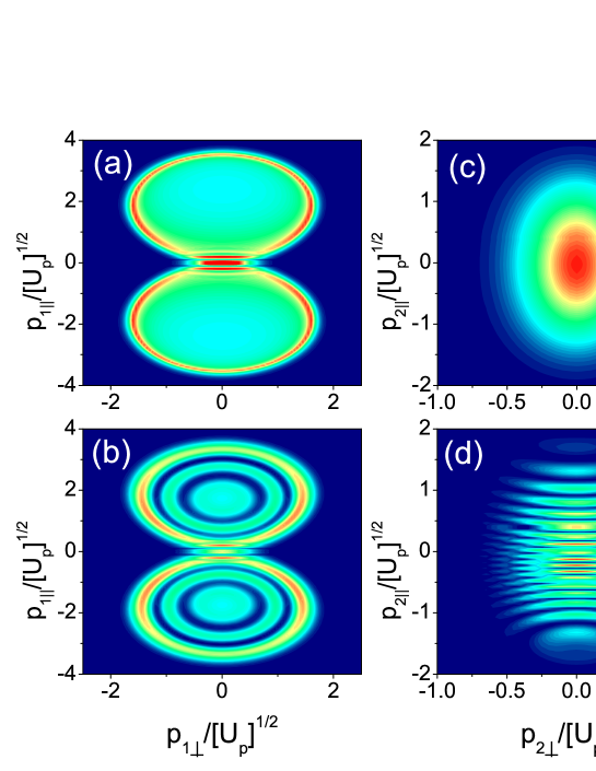
Figure 1: Partial RESI transition probabilities for a monochromatic driving field, as function of the momentum components $p_{1,2\parallel}$ parallel and $p_{1,2\perp}$ perpendicular to the laser field polarization. Panels (a) and (b) depict the transition probability $|M^{(1)}(\mathbf{p}_{1})|^{2}$ for the first electron, Eq. (17), while panels (c) and (d) give the transition probability $|M^{(1)}(\mathbf{p}_{1})|^{2}$ for the second electron, Eq. (18). Panel (a) shows the contribution of the dominant trajectories of the first electron (one per half cycle), while panel (b) shows its interference with the subdominant partner trajectories in the same half cycle, treated collectively in uniform approximation. The trajectory pairs from the two half cycles result in identical distributions for opposite parallel momenta; interference between these pairs of trajectories is negligible. Panel (c) shows the contribution of an individual orbit of the second electron, while panel (d) shows its interference with second orbit in the same field cycle. The distributions have been normalized with regard to the largest value in each panel. Parameters are for Helium ($E^{(g)}_{1}=0.97$ a.u., $E^{(g)}_{2}=2$ a.u. and $E^{(e)}_{2}=0.5$ a.u.), and the driving field is monochromatic with intensity $I=3\times 10^{14}\mathrm{W/cm^{2}}$ and frequency $\omega=0.057$ a.u.

We start with the simpler case of the second electron. For this electron, there are two saddles, whose start times, for vanishing parallel momenta, lie at adjacent field maxima separated by half a cycle of the driving field. Each saddle on its own gives identical contributions to the probability $|M^{(2)}(\mathbf{p}_{2})|^{2}$. These individual contributions are depicted in Fig. 1(c). Figure 1(d) shows the rich interference pattern which arises from the quantum mechanical superposition of the two adjacent saddles. The individual contributions are maximal at $(p_{2\parallel},p_{2\perp})=(0,0)$, for which the effective potential barrier is narrowest and tunneling most probable. These momentum components mark the center of the momentum map. The probability density quickly drops off with increasing momenta $\mathbf{p}_{2}$, i.e., as one moves away from the center of the momentum map. This is expected as the effective potential barrier through which the electron tunnels widens in this case (see discussion of Eq. (16)).

For the first electron, there exist two pairs of saddles. Each pair stems from a half cycle of the field and, for the parameter range employed in the figure, can be associated to a classically allowed region centered at $(p_{2\parallel},p_{2\perp})=(\mp 2\sqrt{U_{p}},0)$ (see discussion of Eq. (14)). Figures 1(a) and (b) show the resulting probability $|M^{(1)}(\mathbf{p}_{1})|^{2}$, calculated either only using the saddle leading to exponentially decaying contributions outside the classical boundary [panel (a)] or the complete pair [panel (b)]. The boundary of the classical region is visible as an outer, bright ring, which indicates the locus of the Stokes transition. If in panel (b) the second saddle would be dropped abruptly beyond the transition one would obtain a cusp. We eliminated this artifact by treating the pair collectively using the uniform approximation Uniform2002 . The remaining fringes are caused by the interference between the two orbits of the pair. In practice, there is only interference between saddles separated by half a cycle around $(p_{1\parallel},p_{1\perp})=(0,0)$, as they mostly populate different momentum regions.

III.2 Few-cycle pulse

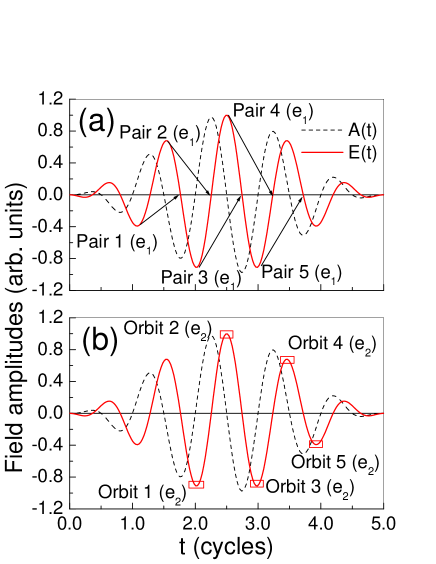
Figure 2: Schematic representation of the electric field $\mathbf{E}(t)$ and the corresponding vector potential $\mathbf{A}(t)$, for a few-cycle pulse of five cycles. The arrows in panel (a) indicate the approximate times around which the first electron leaves, in case it returns at a crossing. The complex return and start times for the indicated pairs of orbits will have real parts in the vicinity of such times. The rectangles in part (b) mark the approximate ionization times for the second electron associated to the orbits utilized in this work (Orbits 1 to 5). The fields have been normalized to $E(t)/E_{0}$ and $A(t)/A_{0}$, where $E_{0}$, $A_{0}$ denote the field amplitudes.

We will now turn to the few-cycle pulse given by Eq. (7), with $N=5$ and carrier envelope phase $\phi=0$. This pulse is shown in Fig. 2, together with the approximate ionization and rescattering times for the first electron, and the ionization times for the second electron [panels (a) and (b), respectively].

The first electron will leave close to an extremum of the field and return near the subsequent field crossing [Fig. 2(a)]. The times indicated in the figure are associated to the real parts of the solutions of the saddle-point equations (11)-(15), for $p_{1\perp}=0$ and $p_{1\parallel}=-A(t^{\prime})$. Each of the five arrows is actually associated to a pair of complex saddle points in the $(t^{\prime\prime},t^{\prime})$ plane. These pairs will be referred to as Pairs $1(e_{1})$ to $5(e_{1})$. Upon recollision, the returning electron will excite a second electron, which will then leave near the subsequent field extremum. The orbits related to these maxima are labeled Orbit $1(e_{2})$ to $5(e_{2})$. The remaining orbits, which are not represented here, will play a negligible role, due to the fact that the ionization times for the first or second electron lie too close to the trailing edges of the pulse. This implies that the corresponding ionization probabilities will be very small. Below, we discuss momentum-space maps for the above-mentioned few-cycle driving pulse.

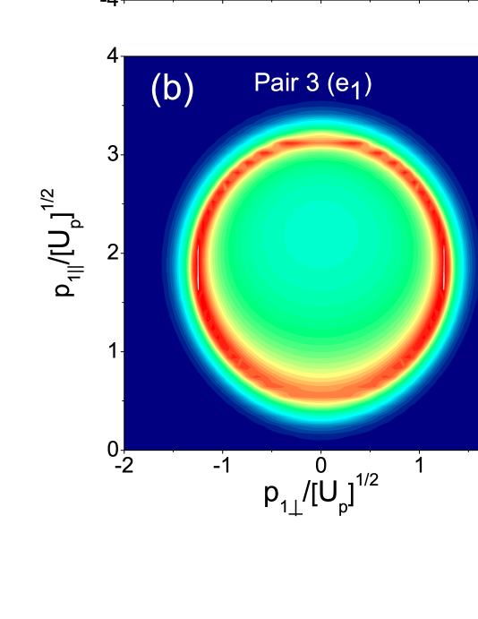
Figure 3: Contributions from specific sets of orbits to the momentum-resolved RESI transition probabilities $|M^{(1)}(\mathbf{p}_{1})|^{2}$ of the first electron, Eq. (17), for the few-cycle pulse of Fig. 2. Panels (a), (b), (c) and (d) correspond to Pairs 2, 3, 4 and 5$(e_{1})$, respectively (to eliminate distorting interference effects, only the dominant orbit, which remains physical beyond the classical boundary, has been taken into account). The pulse has peak intensity $I=2.5\times 10^{14}\mathrm{W/cm^{2}}$, frequency $\omega=0.057$ a.u. and carrier-envelope phase $\phi=0$; the other parameters are the same as in Fig. 1.

We will start by analyzing the transition probability $|M^{(1)}(\mathbf{p}_{1})|^{2}$ for the first electron as a function of $(p_{1\parallel},p_{1\perp}),$ for each of the relevant pairs of orbits indicated in Fig. 2. As in the monochromatic case, a reasonable insight into the relevant momentum range is provided by the orbit in each pair whose contribution decays exponentially outside the classically allowed region. In Fig. 3, we display the contributions of these orbits. As an overall feature, the center of such maps is no longer located at $(p_{1\parallel},p_{1\perp})=(\pm 2\sqrt{U_{p}},0),$ but varies from cycle to cycle. This is due to the fact that this estimate, albeit valid for a monochromatic field, no longer describes a field crossing for a few-cycle pulse. In fact, the exact position of a field crossing will depend on the pulse envelope and on the carrier-envelope phase. Still, the momentum maps remain centered around vanishing transverse momenta $p_{1\perp}.$ This is expected, as the effective widening of the excitation energy for $p_{1\perp}\neq 0$ that can be inferred from Eq. (14) occurs regardless of the shape of the external driving field.

Apart from that, the magnitudes of the partial probabilities $|M^{(1)}(\mathbf{p}_{1})|^{2}$ will vary from cycle to cycle. Whether the contributions of a certain pair will be prominent, irrelevant or even vanishingly small will depend on several issues. If, for instance, the field amplitude is large for a specific cycle, the ionization probability for the first and second electrons are expected to be large as well. Thus, the contributions from orbits starting at such times are expected to prevail. Apart from that, if, for a particular set of orbits, the kinetic energy of the electron upon return is much larger than the energy required to excite the second electron, according to Eq. (13) there will be an extensive classically allowed momentum region. This will also play a role in making the contributions of a particular set of orbits prominent. In the specific case presented here, the contributions from Pair 3$(e_{1})$ and Pair 4$(e_{1})$, depicted in Fig. 3(b) and (c), respectively, are comparable, and at least three orders of magnitude larger than those from the other pairs. This is expected, as the ionization times related to both pairs are very close to the center of the pulse (see Fig. 2). Hence, there is a high tunneling probability for the electron at these times. Further inspection, however, shows that the classically allowed region related to Pair 3$(e_{1})$ is larger. This is related to the kinetic energy the electron exhibits upon return, which is highest for this pair. The contributions of the remaining pairs are less relevant, as the ionization times are closer to the trailing edge of the pulse. For instance, the contributions from Pair 5$(e_{1})$, displayed in Fig. 3(d), are several orders of magnitude smaller than the other pairs. This is due to the fact that for this specific pair of orbits, the first electron does not return with enough kinetic energy to excite the second electron and still reach the detector; hence, rescattering is forbidden throughout. We have verified that this also happens for Pair 1$(e_{1})$. For that reason, we do not include its contributions in the present figure.

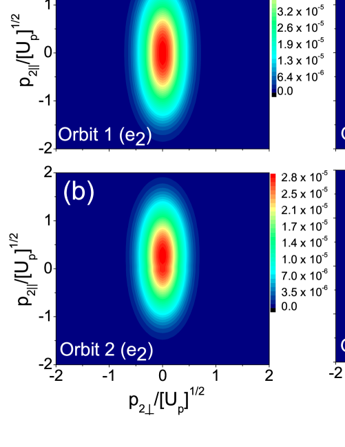
Figure 4: Contributions of individual orbits to the momentum-resolved RESI transition probabilities $|M^{(2)}(\mathbf{p}_{2})|^{2}$ for the second electron, Eq. (18), for the same few cycle pulse and atomic parameters as in Fig. 3. Panels (a), (b), (c) and (d) depict the contributions from the orbits 1, 2, 3 and 4$(e_{2})$, respectively (see Fig. 2).

We will now analyze the partial ionization probability of the second electron by computing $|M^{(2)}(\mathbf{p}_{2})|^{2}$ for Orbits 1-4$(e_{2})$ individually. Fig. 4 shows the outcome of these computations as functions of the parallel and perpendicular momenta $(p_{2\parallel},p_{2\perp})$. Similarly to what has been observed for the first electron, the centers of the momentum-space maps shift away from the position $(p_{2\parallel},p_{2\perp})=(0,0)$. This shift is due to the lack of monochromaticity of the driving field, which introduces an asymmetry around the field extrema and leads to a slight bias towards either the positive or the negative parallel momentum region. This bias is more pronounced for orbits whose ionization times approach the trailing edge of the pulse. For the specific pulse considered in this work, this can be observed in the contributions from Orbits 3$(e_{2})$ and 4$(e_{2})$ [Fig. 4(c) and (d), respectively]. Still, for all cases, the momentum-space maps remain centered at $p_{2\perp}=0.$ This is a consequence of the fact that, effectively, the potential barrier through which the electron must tunnel is narrowest in this case, regardless of the shape of the field (see discussion of Eq. (16)).

Furthermore, the closer the ionization time is to the pulse center, the larger the contributions from the corresponding orbit will be. For the specific pulse considered here, for instance, the contributions from Orbit 1$(e_{2})$ and Orbit 2$(e_{2})$, displayed in Figs. 4(a) and (b), respectively, are at least one order of magnitude larger than those of the remaining orbits. In the figure, we do not include the contributions from Orbit 5$(e_{2})$, as these are at least four orders of magnitude smaller than those of the remaining orbits.

As in the monochromatic-field case, the contributions of the above-stated sets of orbits must be added coherently. This will lead to interference maxima and minima, both in the momentum maps and in the electron-momentum distributions. In Fig. 5, we display the momentum maps for the first and the second electron (left and right panels, respectively). The upper and lower panels, respectively, exhibit the contributions of the dominant sets of orbits, i.e., Pairs $3(e_{1})$ and $4(e_{1})$, and Orbits $1(e_{2})$ and $2(e_{2})$, and the overall partial momentum maps, in which all orbits have been included.

Figs. 5(a) and (b) exhibit two circular regions for which the partial probability density is non-vanishing. These regions are roughly centered at $(p_{1\parallel},p_{1\perp})=(\pm 2\sqrt{U_{p}},0)$. Slight displacements away from these points are again related to the lack of monochromaticity of the field. The negative parallel momentum region is dominated by the contributions of Pair $4(e_{1})$. In fact, due to the large tunneling probability associated with it, it leads to the brightest spot in these panels. This pair interferes with Pair $2(e_{1})$, which is temporally displaced by a full cycle of the driving field; this interference is visible as the substructure in Fig. 5(b). The positive parallel momentum region is dominated by Pair $3(e_{1})$. In both panels, one may identify well-defined annular fringes, which are caused by the interference between the long and the short orbit of Pair $3(e_{1})$. These orbits are temporally close, and their contributions are several orders of magnitude larger than those of the remaining pairs $1(e_{1})$ and $5(e_{1})$.

The interference scenario is different for the second electron. In this case, orbits located near different half cycles of the field lead to contributions in overlapping momentum-space regions, roughly centered at $(p_{2\parallel},p_{2\perp})=(0,0)$. For instance, in Fig. 5(c), inclusion of the dominant Orbits $1(e_{2})$ and $2(e_{2})$ already leads to a rich interference pattern. Additional substructures appear if the remaining orbits considered in Fig. 4 are taken into consideration, as shown in Fig. 5(d).

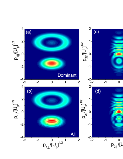
Figure 5: Partial transition probabilities for a few-cycle pulse, as function of the momentum components $p_{n\parallel}$ and $p_{n\perp}$. Panels (a) and (b) depict the partial transition probability $|M^{(1)}(\mathbf{p}_{1})|^{2}$ for the first electron, while panels (c) and (d) depict $|M^{(2)}(\mathbf{p}_{2})|^{2}$ for the second electron. These are obtained by coherently adding the contributions of orbits addressed in Figs. 3 and 4 (the field and atomic parameters are the same as in these figures). In panels (a) and (c), this sum is restricted to the dominant orbits of pairs $3(e_{1})$ and $4(e_{1})$, as well as $1(e_{2})$ and $2(e_{2})$, respectively. The distributions have been normalized with regard to the maximum probability density in each panel.

IV Causality for complex times

In this section, we describe how the fact that ionization of the second electron must be subsequent to the rescattering of the first electron reflects itself in the complex time plane, and exemplify this for a monochromatic driving field and a few-cycle pulse. This construction forms the basis of the calculation of correlated RESI momentum distributions, which are presented in Sec. V.

Causality in the classical sense means that the first electron rescatters with the core prior to the second electron being freed. If both the rescattering time $t^{\prime}$ of the first electron and the ionization time $t$ of the second electron were real, this condition would simply require $t^{\prime}<t$. This condition is also embodied in the integration range of the SFA expression (1) for the transition amplitude. However, because tunneling is not a classical process, the solutions of the saddle-point equations  (11)-(15) are complex. Hence, in order to evaluate the integrals in terms of these orbits one must determine how causality manifests itself in the complex plane.

This can be done by reinspecting the steps that lead to the saddle point approximation of the RESI transition amplitude (1). This amplitude can be rewritten as

$$M(\mathbf{p}_{1},\mathbf{p}_{2})$$ (20)

$$=\int_{-\infty}^{\infty}dt^{\prime\prime}\int_{t^{\prime\prime}}^{\infty}dt^{\prime}\int d^{3}kV_{\mathbf{p}_{1},\mathbf{k}}^{(eg)}V_{\mathbf{k}}^{(g)}e^{iS_{1}(\mathbf{p}_{1},\mathbf{k},t^{\prime\prime},t^{\prime})}M^{(2)}(\mathbf{p}_{2};t^{\prime}),$$

whereupon the time-conditioned amplitude

$$M^{(2)}(\mathbf{p}_{2};t^{\prime})=\int_{t^{\prime}}^{\infty}dtV_{\mathbf{p}_{2}}^{(e)}e^{iS_{2}(\mathbf{p}_{2},t)}$$ (21)

of the second electron depends on the rescattering time $t^{\prime}$ via the lower integration limit and is part of an integrand, in contrast to the partial amplitude $M^{(2)}(\mathbf{p}_{2})=M^{(2)}(\mathbf{p}_{2};-\infty)$, Eq. (18), evaluated in Sec. III.

Let us assume that we have integrated out ${\bf k}$ via a saddle point approximation (which is exact if one neglects the ${\bf k}$ dependence of the form factors) and denote the resulting effective action as $\tilde{S}(\mathbf{p}_{1},\mathbf{p}_{2},t^{\prime\prime},t^{\prime},t)$. We then can deform the integration manifold over the three times $t^{\prime\prime}$, $t^{\prime}$ and $t$ into the complex plane. The integrand can be analytically continued and does not possess any poles. Therefore, the value of the integral does not change by this deformation. In the steepest-descent method Bleistein , this deformation is carried out such that the quickly oscillating part $e^{i\tilde{S}(\mathbf{p}_{1},\mathbf{p}_{2},t,t^{\prime},t^{\prime\prime})}$ of the integrand changes into a smooth expression with maxima around the saddle points. To this end one associates to each saddle $(t^{\prime\prime}_{a},t^{\prime}_{a},t_{a})$ a sheet on which $\mathrm{Re}\,\tilde{S}(\mathbf{p}_{1},\mathbf{p}_{2},t,t^{\prime},t^{\prime\prime})=\mathrm{Re}\,\tilde{S}(\mathbf{p}_{1},\mathbf{p}_{2},t_{a},t^{\prime}_{a},t^{\prime\prime}_{a})$. (In more than one dimension, these sheets are not unique, but this does not affect any results howls .) Different sheets can meet in zeros of the integrand, since there the phase is not well defined. Sheets have to be joined such that the total deformed manifold starts and ends at the original lower and upper integration limits of the integral, respectively. Therefore, one also needs sheets connected to these boundaries, which are again constructed such that the integrand decays rapidly as one moves away from the integration limits. Following this prescription, not all saddle sheets will be part of the total deformed manifold, which means that only a restricted set of all saddles is contributing to the final expression. The saddle point approximation follows by expanding $\tilde{S}$ around the maxima or integration limits, so that one obtains simple integrals for each saddle point on the total contour, as well as each boundary sheet. These individual contributions are accurate approximations if the saddles and integration limits are not too close to each other; otherwise one needs to employ uniform approximations.

In order to apply this procedure to Eqs. (20), (21), we proceed in three interlinked steps.

(I) Consider the time-conditioned amplitude $M^{(2)}(\mathbf{p}_{2};t^{\prime})$. The saddles in the complex $t$ plane are the same as for the partial amplitude (18), and therefore determined by condition (15). However, the steepest descent contour now depends on the integration limit $t^{\prime}$, as we have to construct a continuous contour in the complex $t$ plane that links it to the upper integration limit (at real $+\infty$). The contour therefore starts with a segment of fixed $\mathrm{Re}[S_{2}(\mathbf{p}_{2},t)]=\mathrm{Re}[S_{2}(\mathbf{p}_{2},t^{\prime})]$. This boundary segment has then to be linked with contour segments passing through saddles $t_{a}$, for which $\mathrm{Re}[S_{2}(\mathbf{p}_{2},t)]=\mathrm{Re}[S_{2}(\mathbf{p}_{2},t_{a})]$. Compared to the calculation of the unconditioned amplitude $M^{(2)}(\mathbf{p}_{2})$, this has two effects: (i) There is an additional contribution from the boundary segment linked to $t^{\prime}$, which we will neglect as it is related to the electron-impact pathway NSDI2004_1 and (ii) only a subset of saddles $t_{a}$ contributing to $M^{(2)}(\mathbf{p}_{2})$ will lie on the contour conditioned by starting at $t^{\prime}$. Besides this selection criterion, the individual saddle point contributions do not explicitly depend on $t^{\prime}$. However, the number of relevant saddles changes at Stokes transitions, which for a given saddle $t_{a}$ occur when $\mathrm{Re}[S_{2}(\mathbf{p}_{2},t^{\prime})]=\mathrm{Re}[S_{2}(\mathbf{p}_{2},t_{a})]$. (This condition is not sufficient; whether there is indeed a Stokes transition can be verified by constructing the explicit integration contour, as carried out below.)

(II) Next, we apply the saddle point approximation to the remaining integrals over $t^{\prime\prime}$ and $t^{\prime}$. We will focus at situations not too close to a Stokes transition. Within a range in $t^{\prime}$, the contributions from the saddle points of $M^{(2)}(\mathbf{p}_{2};t^{\prime})$ will then not depend on $t^{\prime}$. Therefore, this term can be treated as approximately constant, and will not affect the saddle point conditions (11)-(13) for $t^{\prime\prime}$ and $t^{\prime}$.

(III) This in turn means that we now can substitute the lower integration limit in $M^{(2)}(\mathbf{p}_{2};t^{\prime})$, which was considered general so far, with the values of complex saddle points $t^{\prime}_{b}$.

As an upshot, we find that for each saddle point trajectory ($t^{\prime\prime}_{b},t^{\prime}_{b}$) of the first electron, only a certain number of saddle points $t_{a}$ of the second electron will contribute. These are the ones that lie on the continuous steepest descend contour in the complex $t$ plane that starts at the rescattering time $t^{\prime}_{b}$ of the first electron. Since the saddle-point values $t^{\prime}_{b}$ depend on the momentum $\mathbf{p}_{1}$ of the first electron, but the remainder of the complex $t$ contour (and in particular the location of the saddles $t_{a}$) depends on the momentum $\mathbf{p}_{2}$ of the second electron, this generalized causality requirement results in additional correlations for the momentum distributions, which will be quantified in the following Sec. V. In the remainder of this section we focus on the explicit construction of the described steepest descent contours.

IV.1 Steepest descent contours for monochromatic driving

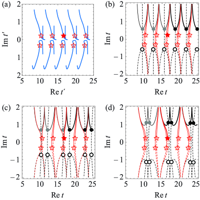
Figure 6: Construction of steepest descent contours for the evaluation of $M^{(2)}(\mathbf{p}_{2};t^{\prime})$, Eq. (21), for monochromatic driving, with complex rescattering times $t^{\prime}$ corresponding to $p_{1\perp}=0$, $p_{1\parallel}=0$. In panel (a), these rescattering times, obtained by solving the saddle point equations (11)-(13), are indicated by the star symbols. For orientation, the curves show the trace of times $t^{\prime}$ when $p_{1\parallel}$ is varied from $-5\sqrt{U_{p}}$ to $+5\sqrt{U_{p}}$ while $p_{1\perp}=0$ remains fixed. In panels (b)-(d), the circles indicate the ionization times $t$ of the second electron for $p_{2\perp}=0$, while the parallel momentum takes the values $p_{2\parallel}=0$ (panel b), $p_{2\parallel}=1.5\sqrt{U_{p}}$ (panel c), and $p_{2\parallel}=3\sqrt{U_{p}}$ (panel d), respectively. These times are obtained by solving the saddle point equation (15). The solid circles indicate saddles that are physically allowed (with positive ${\rm Im}\,S_{2}$), while the open circles are unphysical. The dark solid lines indicate the steepest descent contour through these saddles, while the dark dashed lines indicate steepest ascent contours, as well as steepest descent contour through unphysical saddles. The red (light) lines are steepest descent contours passing through the rescattering times $t^{\prime}$ (star symbols). These lines are all determined from the condition ${\rm Re}\,S_{2}={\rm const}$. A full steepest descent contour must make use of solid lines in order to connect a lower integration limit $t=t^{\prime}$ (stars) to the upper integration limit (at $t=+\infty$). The thick lines show the full contour for one selected starting value, indicated by the solid star. This contour only visits a selection of all physical saddles (dark dots). Between panels (c) and (d) a Stokes transition occurs, where an additional saddle becomes accessible.

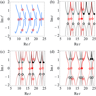
Figure 7: Construction of steepest descent contours as in Fig. 6, but for rescattering times corresponding to $p_{1\perp}=0$, $p_{1\parallel}=2\sqrt{U_{p}}$. Due to this change, in every cycle one pair of rescattering times moves closer to the real axis, corresponding to physically allowed rescattering, while the other pair moves away from the real axis. The initial values of the steepest descent contours in panels (b)-(d) are therefore shifted. For the rescattering time indicated by the solid star, again a Stokes transition occurs, but now a saddle is lost, not gained.

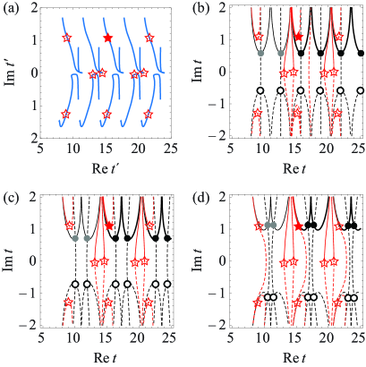
Figure 8: Same as Fig. 6, but for rescattering times corresponding to $p_{1\perp}=0$, $p_{1\parallel}=-2\sqrt{U_{p}}$. In comparison to Fig. 7, the rescattering times are shifted by a half cycle. The rescattering time indicated by the solid star now corresponds to a negligible contribution (its partner saddle is unphysical) and does not exhibit a Stokes transition.

Steepest descent contours for monochromatic driving and different combinations of momenta are shown in Figs. 6-8. In order to identify the starting point of such contours, we show in panel (a) of each figure the rescattering times $t^{\prime}$ of the first electron (star symbols), corresponding to $(p_{1\parallel},p_{1\perp})=(0,0)$ in Fig. 6, $(p_{1\parallel},p_{1\perp})=(2\sqrt{U_{p}},0)$ in Fig. 7, and $(p_{1\parallel},p_{1\perp})=(-2\sqrt{U_{p}},0)$ in Fig. 8 (according to Fig. 1, these values corresponds to the point midway between the maxima in the momentum map, as well as the locations of these maxima). Panels (b)-(d) of Figs. 6-8 show these values as integration limits in the $t$ plane, along with the complex ionization times of the second electrons (dots). In all panels $p_{2\perp}=0$, while the parallel momentum takes the values $p_{2\parallel}=0$ (panel b), $p_{2\parallel}=1.5\sqrt{U_{p}}$ (panel c), and $p_{2\parallel}=3\sqrt{U_{p}}$ (panel d), respectively [according to Fig. 1, panel (b) therefore corresponds to the maximum in the momentum map of the second electron]. The solid lines in these plots show steepest descent segments from which a full contour must be constructed. These only pass saddles in the upper half plane (solid dots), as the saddles in the lower half plane (open dots) have ${\rm Im}\,S_{2}<0$. They will lead to exponentially increasing contributions and therefore are unphysical. However, for a given starting value not all the physical saddles are visited. This is illustrated by sample contours (thick lines) that start at a selected rescattering time, indicated by the solid star, and only pass the saddles indicated by the dark dots, while the gray solid dots are left out.

In this way, for any given saddle-point rescattering time $t^{\prime}$ we can define a clear boundary in the complex $t$ plane that determines whether a saddle-point ionization time is allowed by causality or not. This boundary passes over saddles whenever a Stokes transition occurs. The thick sample contours display a Stokes transition in Figs. 6 and 7, but not in 8.

Inspecting these figures more generally, we see that to a good approximation, the causality requirement assumes the form ${\rm Re}\,t^{\prime}<{\rm Re}\,t$. This is the case because Stokes transitions take place when a start time $t^{\prime}$ crosses over the steepest-ascent segment of a physically allowed ionization time $t$. In the figures, these lines are seen to lead almost vertically from a physical saddle in the upper half of the complex-$t$ plane to an unphysical mirror saddle in the lower half plane. We verified that this approximate causality criterion remains valid over the range of momenta where the momentum maps in Fig. 1 are large.

IV.2 Steepest descent contours for a few-cycle pulse

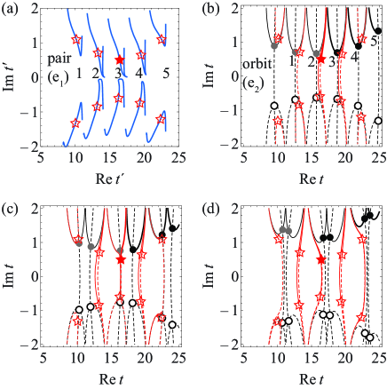
Figure 9: Construction of steepest descent contours as in Fig. 6, but for a few cycle pulse. Labels refer to the orbit pairs (first electron) and orbits (second electron) indicated in Fig. 2. Panel (a) shows the effect of the finite pulse length on the first electron. The stars again denote the rescattering times for $p_{1\perp}=0$, $p_{1\parallel}=0$. In the tails of the pulse the driving is weak, resulting in rescattering times that are shifted away from the real axis. Therefore, some of these trajectories of the first electron become negligible. Panels (b)-(d) show that the same effect also occurs for the ionization times $t$ of the second electron. The solid star indicates a rescattering time in the center of the pulse, which gives the largest semiclassical contribution. The value of this time is close to that in the monochromatic case, and the associated steepest descent contours (thick lines) display the same type of Stokes transition as in that case (cf. Fig. 6).

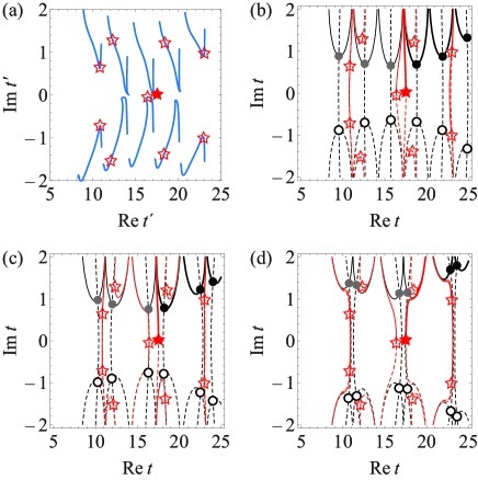
Figure 10: Construction of steepest descent contours for a few cycle pulse as in Fig. 9, but corresponding to $p_{1\perp}=0$, $p_{1\parallel}=2\sqrt{U_{p}}$, for which the rescattering time indicated by the solid star moves closer to the real axis. In comparison to the monochromatic case in Fig. 7, the associated steepest descent contours again display the same type of Stokes transition.

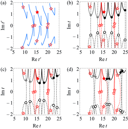
Figure 11: Same as Fig. 9, but for rescattering times corresponding to $p_{1\perp}=0$, $p_{1\parallel}=-2\sqrt{U_{p}}$. As in the monochromatic case (Fig. 8), the rescattering time indicated by the solid star now corresponds to a negligible contribution and does not exhibit a Stokes transition.

Figures 9-11 show the corresponding steepest descent contours for the few cycle pulse. Instead of a periodic repetition cycle-by-cycle, the rescattering times (stars) and ionization times (dots) are now modulated according to their position in the pulse (see Sec. III.2 and Fig. 2). In the tails of the pulse, where the intensity is small, the rescattering and ionization times move away from the real axis. Compared to the monochromatic case, the steepest descent contours are therefore distorted, but the main features are still strikingly similar. In particular, we observe the same type of Strokes transitions, and the simplified causality criterion ${\rm Re}\,t^{\prime}<{\rm Re}\,t$ is clearly still a good approximation. However, from these figures we can still anticipate that the causality constraint in itself plays a much more significant role when it comes to the calculation of actual transition probabilities. Large contributions to the momentum yield should stem from the saddle points close to the center of the pulse. Because of the causality constraint, however, it is not always possible to combine the most favorable rescattering and ionization times. In the figures, this is illustrated by the sample contours, which start at the rescattering time $t^{\prime}$ of the long orbit in pair $4(e_{1})$ (the most favorable time according to Fig. 3). The most favorable ionization time for the second electron is that of orbit $2(e_{2})$ (see Fig. 4), but these orbits generally cannot be combined because of causality. In the following section, we quantify the consequences in terms of the correlated momentum distributions of both electrons.

V Momentum distributions

In this section we compute two-electron momentum distributions as functions of the momentum components $(p_{1\parallel},p_{2\parallel})$ parallel to the laser field polarization, contrasting again the case of a monochromatic field to that of a few cycle pulse. For both cases, we calculate the momentum distribution for resolved parallel and restricted ranges of the transverse momenta. If transverse momenta are fully integrated out, as it is done in many NSDI studies, quantum-interference effects get washed out and causality-related effects can no longer be identified. This also holds for cusps or further artifacts that may be present in saddle-point approximations, and which indicate their breakdown. Hence, transverse momentum integration would mask the very effects we intend to analyze.

We consider the distributions

$$F(p_{1\parallel},p_{2\parallel})=\int^{p^{(\mathrm{max})}_{1\perp}}_{p^{(\mathrm{min})}_{1\perp}}\int^{p^{(\mathrm{max})}_{2\perp}}_{p^{(\mathrm{min})}_{2\perp}}d^{2}p_{1\perp}d^{2}p_{2\perp}|M(\mathbf{p_{1}},\mathbf{p_{2}})+\mathbf{p_{1}}\leftrightarrow\mathbf{p_{2}}|^{2},$$ (22)

which have been symmetrized with regard to electron exchange. This is necessary as the two electrons are indistinguishable. In the above-stated equation, $p^{(\mathrm{min})}_{n\perp}$ and $p^{(\mathrm{max})}_{n\perp}$ $(n=1,2)$ denote the minimal and the maximal transverse momenta to be taken into account.

For a monochromatic driving field, the causality-induced shielding of saddles does not have an observable effect on the momentum distributions. This is so because the saddles are repeating periodically cycle by cycle, and all have to be added coherently,. This eventually results in a closely spaced train of delta functions which embody the Bohr resonance condition for multiple-photon absorption kopold . Smoothing over these delta functions, we find $M(\mathbf{p}_{1},\mathbf{p}_{2})=M^{(1)}(\mathbf{p}_{1})M^{(2)}(\mathbf{p}_{2})$ as if causality had been ignored. For a few-cycle pulse, however, the orbits in different cycles are not equivalent, and casuality has observable consequence. This is demonstrated in Fig. 12, where we present the distributions $F(p_{1\parallel},p_{2\parallel})$ for a monochromatic field (upper panels) and a few-cycle pulse (middle panels ignoring causality, and lower panels respecting casuality), for increasing transverse momenta (left panels: ‘low momenta’ $0<p_{1\perp},p_{2\perp}<0.2\sqrt{U_{p}}$; middle panels: ‘medium momenta’ $0.6\sqrt{U_{p}}<p_{1\perp},p_{2\perp}<0.8\sqrt{U_{p}}$; right panels panels: ‘large momenta’ $\sqrt{U_{p}}<p_{1\perp},p_{2\perp}<1.2\sqrt{U_{p}}$).

For the monochromatic driving field, Figs. 12(a)-(c), all distributions adhere to the momentum constraints defined for RESI SF2010 , i.e., they are cross-shaped and located along the axes $p_{n\parallel}=0$ $(n=1,2)$. The elongation of such distributions is determined by the saddle-point equation (14), which yields the momentum-space regions filled by the rescattering of the first electron, and the width of such distributions is given by the maximal and minimal momenta determined by Eq. (16). They are also symmetric upon the reflection $p_{n\parallel}\rightarrow-p_{n\parallel}$, which is a direct consequence of the time-reversal symmetry of the field. This means that, without symmetrization upon electron exchange, these distributions would be located along the horizontal axis $p_{1\parallel}=0$. The symmetrization $\mathbf{p}_{1}\leftrightarrow\mathbf{p}_{2}$ leads to the vertical axis of the crosses. The rather rich substructure present in the figure is associated to the quantum interference between the long and short orbit for the first electron, and between orbits displaced by half a cycle for the second electron.

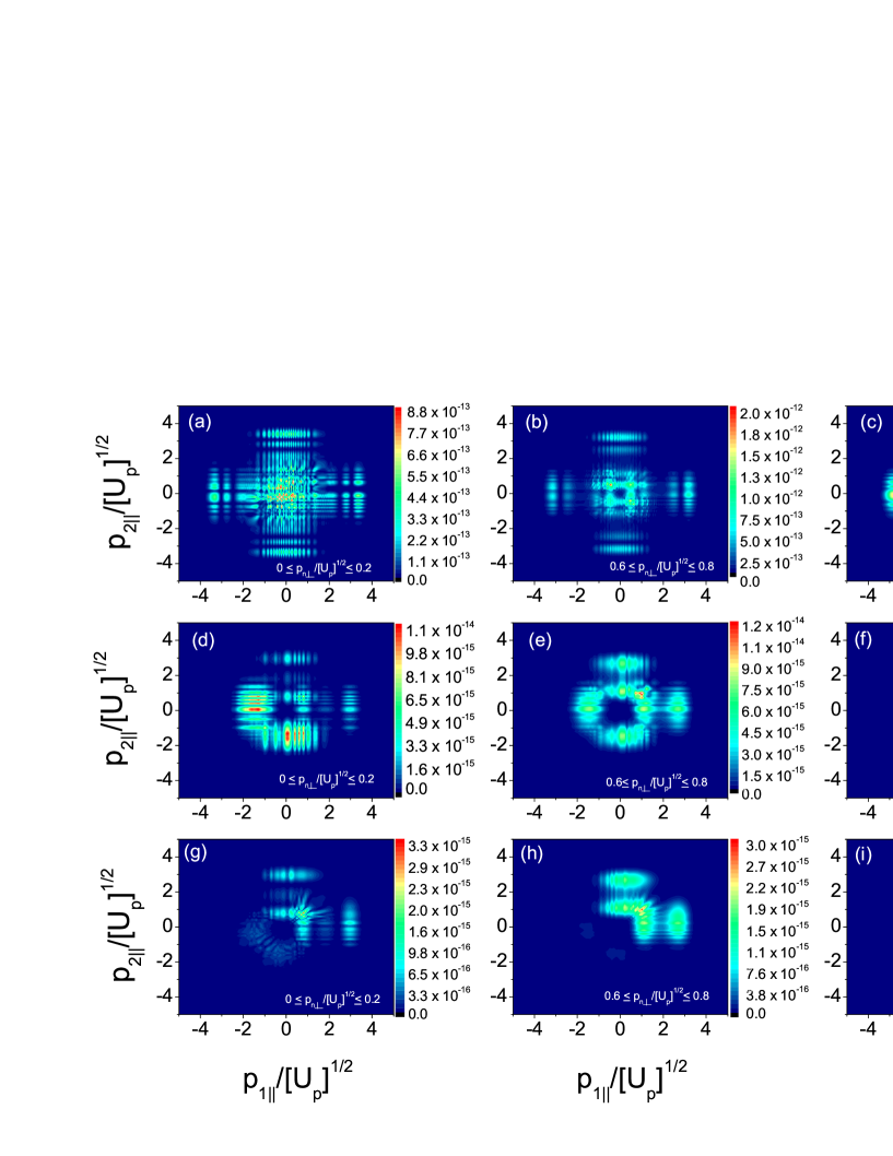
Figure 12: Correlated RESI two-electron momentum distributions $F(p_{1\parallel},p_{2\parallel})$ as functions of the electron momentum components $p_{n\parallel}$ ($n=1,2$) parallel to the laser-field polarization. The atomic parameters correspond to Helium (see Fig. 1). Panels (a) to (c) have been computed for a monochromatic field of intensity $I=3\times 10^{14}\mathrm{W/cm}^{2}$ and frequency $\omega=0.057$ a.u., while in panels (d) to (i) a five-cycle pulse of intensity $I=2.5\times 10^{14}\mathrm{W/cm}^{2}$, frequency $\omega=0.057$ a.u. and carrier-envelope phase $\phi=0$ has been used. The middle row of panels (d)-(f) show results for the few-cycle pulse if causality is discarded (these results are therefore unphysical), while the bottom panels (g)-(i) show the results for the few-cycle pulse including the causality restrictions. From the left to the right column of panels, we integrated over a transverse momentum range centered around low, medium, and large transverse momenta, respectively.

For a few-cycle pulse, in contrast, the electron momentum distributions are very much affected by causality. To isolate these effects, we start by analyzing the situation if causality could be neglected, displayed in Figs. 12(d), (e) and (f). These distributions are again obtained by assuming $M(\mathbf{p}_{1},\mathbf{p}_{2})=M^{(1)}(\mathbf{p}_{1})M^{(2)}(\mathbf{p}_{2})$. The distributions are then asymmetric, which is a direct consequence of the asymmetries in the momentum maps in Fig. 5. The momentum maps are localized in the momentum region determined by the dominant orbits, located close to the center of the pulse. For low transverse momenta, the contribution from Pair $4(e_{1})$ dominates in $M^{(1)}(\mathbf{p}_{1})$, which in Fig. 5(a,b) gives rise to the bright spot at $(p_{1\parallel},p_{1\perp})=(-2\sqrt{U_{p}},0)$. Hence, one expects the distribution to be located in the region $-2\sqrt{U_{p}}\leq p_{2\parallel}\leq 2\sqrt{U_{p}}$ along the negative $p_{1\parallel}$ half axis. Symmetrization upon electron exchange leads to the occupation of the momentum-space region around the negative $p_{2\parallel}$ half axis, with $-2\sqrt{U_{p}}\leq p_{1\parallel}\leq 2\sqrt{U_{p}}$.

For medium transverse momenta the contribution from Pair $3(e_{1})$ [corresponding in Fig. 5(a,b) to the bright ring for $p_{1\parallel}>0$] becomes comparable to that of Pair $4(e_{1})$. Consequently, the two-electron distribution in Fig. 12(e) spreads out in the parallel momentum plane. Indeed, the contributions around the positive half axes $p_{n\parallel}>0$ $(n=1,2)$ are now comparable to those along the negative half axes. For large transverse momenta (Fig. 12(f)), Pair $3(e_{1})$ dominates over $4(e_{1})$, and the distributions moves into the half positive axes. Apart from that, the results show that, the larger the transverse momentum range is, the more concentrated around $p_{n\parallel}=2\sqrt{U_{p}}$ the electron momentum distributions are.

Up to the present stage, however, causality has not been taken into account. For instance, the largest contributions to the partial momentum maps for the first and second electron [Pair $4(e_{1})$ and Orbit $2(e_{2})$, respectively], are not connected by causality, and therefore their combined contribution must be discarded. Indeed, the most favorable overall RESI pathway arises from combining Pair $3(e_{1})$ with Orbits $2(e_{2})$ (if accessible) and $3(e_{2})$. The large contribution related to Pair $4(e_{1})$ is not sufficient to counter-act the lower tunneling probabilities related to Orbits $4(e_{2})$ and $5(e_{2})$. Figs. 12(g) to (i) illustrate the consequences. Since Pair $3(e_{1})$ results in a large yield at $p_{1\parallel}>0$, the electron momentum distributions are now mostly concentrated along the positive half axes $p_{n\parallel}$ $(n=1,2)$. This situation persists over all transverse momentum ranges.

Apart from the reshaping of the distributions, a noteworthy feature in Fig. 12 is an overall decrease of a few orders of magnitude in comparison to the situation in which causality has been disregarded. Taken altogether, these results show that causality has a drastic effect on the two-electron momentum distributions in the RESI pathway.

VI Conclusions

In this work we performed a detailed analysis of the recollision with subsequent tunneling ionization (RESI) mechanism in laser-induced nonsequential ionization (NSDI), with emphasis on the implications of causality. Physically, RESI means that the first electron rescatters with the core at an instant $t^{\prime}$ and excites a second electron, which tunnel ionizes at a subsequent time $t$. Causality means that tunnel ionization of the second electron can only occur after the recollision of the first electron. Applying the saddle point approximation to the strong-field expressions, the rescattering and ionization times become complex (since tunneling does not have a classical counterpart), and the notion of causality has to be generalized into the complex time plane. We have shown that the concepts of “before” and “after” translate into boundary conditions limiting the steepest-descent contours to be taken. These boundary conditions are given by the complex rescattering times of the first electron. Ionization times of the second electron are casually connected to a rescattering event if it lies on a steepest descent contour that connects the rescattering time to the distant future. In practice, this often translates into a simple rule where only the real parts of the complex times have to be compared. Deviations have been observed, however, for pairs of electron orbits associated with the trailing edge of the pulse, or for momentum regions in which the RESI yield is strongly suppressed.

We illustrated the influence of causality and quantum-interference on momentum-resolved two-electron distributions. In order to isolated these effects, we compared distributions for a monochromatic driving field to those for a few-cycle pulse. While causality does not affect the electron momentum distributions obtained for monochromatic fields, it significantly affects the results for a few-cycle pulse. For these pulses, there exist several competing sets of orbits, whose dominance influences the shapes of the electron momentum distributions, which generally are highly asymmetric and concentrated in specific momentum regions. Causality puts constraints on the construction of two-electron trajectories, which drastically changes the momentum regions populated by the distributions.

Causality may have consequences even for monochromatic driving when it is combined with additional effects, such as bound-state depletion. Depending on the laser-field intensity and the binding energy of the excited state, such depletion can be considerable, and if this is the case the ionization time $t$ lying closest in the future of the rescattering time $t^{\prime}$ is expected to contribute most. Such effects go beyond the present work, but may warrant further investigation.

VII Acknowledgements

This work was funded by the UK EPSRC (Grant no EP/D07309X/1) and by the UCL/EPSRC PhD+ scheme. T.S. and C.F.M.F. would like to thank Lancaster University for its kind hospitality.

References

- (1) P. B. Corkum, Phys. Rev. Lett. 71, 1994 (1993).
- (2) P. Antoine, A. L’Huillier, and M. Lewenstein, Phys. Rev. Lett. 77, 1234 (1996).
- (3) See, e.g., F. Krausz and M. Ivanov, Rev. Mod. Phys. 81, 163 (2009).
- (4) L. V. Keldysh, Sov. Phys. JETP 20, 1307 (1965); F.H.M. Faisal, J. Phys. B 6, 289 (1973); H. R. Reiss, Phys. Rev. A 22, 1786 (1980).
- (5) M. Lewenstein, Ph. Balcou, M. Yu. Ivanov, A. L’Huillier and P. B. Corkum, Phys. Rev. A 49, 2117 (1994); W. Becker, S. Long, and J. K. McIver Phys. Rev. A Phys. Rev. A 41, 4112 (1990), ibid. 50, 1540 (1994); A. Lohr, M. Kleber, R. Kopold, and W. Becker, Phys. Rev. A 55, R4003 (1997).
- (6) See, e.g., P. Salières, B. Carré, L. Le Déroff, F. Grasbon, G. G. Paulus, H. Walther, R. Kopold, W. Becker, D. B. Milošević, A. Sanpera, and M. Lewenstein, Science 292, 902 (2001) and references therein.
- (7) H. Schomerus and M. Sieber, J. Phys. A 30, 4537 (1997).
- (8) C. Figueira de Morisson Faria, H. Schomerus and W. Becker, Phys. Rev. A 66, 043413 (2002).
- (9) See, e.g., S. Odzak and D. B. Milošević, Phys. Rev. A 72, 033407 (2005); D. B. Milošević, D. Bauer and W. Becker, J. Mod. Opt. 53, 125 (2006); T. K. Kjeldsen and L. B. Madsen, Phys. Rev. A 72, 023407 (2006); C. Figueira de Morisson Faria, Phys. Rev. A 76, 043407 (2007); G. Sansone, Phys. Rev. A 79, 053410 (2009); C. Figueira de Morisson Faria and B. B. Augstein, Phys. Rev. A 81, 043409 (2010); S. Sukiasyan, S. Patchkovskii, O. Smirnova, T. Brabec and M. Ivanov, Phys. Rev. A 82, 043414 (2010); L. E. Chipperfield, J. S. Robinson, P. L. Knight, J. P. Marangos and J. W. G. Tisch, Laser and Phot. Rev. 4, 697 (2010).
- (10) C. Figueira de Morisson Faria, X. Liu, H.Schomerus and W. Becker, Phys. Rev. A 69, 012402(R)(2004); C. Figueira de Morisson Faria, H. Schomerus, X. Liu and W. Becker, Phys. Rev. A 69, 043405 (2004).
- (11) C. Figueira de Morisson Faria and M. Lewenstein, J. Phys. B 38, 3251 (2005).
- (12) X. Liu and C. Figueira de Morisson Faria, Phys. Rev. Lett. 92, 133006 (2004); C. Figueira de Morisson Faria, X. Liu, A. Sanpera and M. Lewenstein, Phys. Rev. A 70, 043406 (2004).
- (13) A. Staudte, C. Ruiz, M. Schoffler, S. Schössler, D. Zeidler, Th. Weber, M. Meckel, D. M. Villeneuve, P. B. Corkum, A. Becker, and R. Dörner. Phys. Rev. Lett. 99, 263002 (2007).
- (14) A. Rudenko, V. L. B. de Jesus, Th. Ergler, K. Zrost, B. Feuerstein, C. D. Schröter, R. Moshammer, and J. Ullrich, Phys. Rev. Lett. 99, 263003 (2007).
- (15) D. I. Bondar, W. K. Liu, and M. Y. Ivanov. Phys. Rev. A 79, 023417 (2009).
- (16) E. Eremina, X. Liu, H. Rottke, W. Sandner, A. Dreischuh, F. Lindner, F. Grasbon, G.G. Paulus, H. Walther, R. Moshammer, B. Feuerstein, and J. Ullrich, J. Phys. B 36, 3269 (2003); Y. Liu, S. Tschuch, A. Rudenko, M. Dürr, M. Siegel, U. Morgner, R. Moshammer, and J. Ullrich, Phys. Rev. Lett. 101, 053001 (2008); Y. Liu, D. Ye, J. Liu, A. Rudenko, S. Tschuch, M. Dürr, M. Siegel, U. Morgner, Q. Gong, R. Moshammer, and J. Ullrich, Phys. Rev. Lett. 104, 173002 (2010).
- (17) See, e.g., S. L Haan, L. Breen, A. Karim, and J. H. Eberly, Phys. Rev. Lett. 97, 103008 (2006); D.F. Ye and J. Liu, Phys. Rev. A 81, 043402 (2010); D. I. Bondar, G. L. Yudin, W.-K. Liu, M. Yu. Ivanov, and A. D. Bandrauk, Phys. Rev. A 83, 013420 (2011); A. Emmanouilidou, J. S. Parker, L. R. Moore and K. T. Taylor, New J. Phys 13, 043001 (2011).
- (18) C. Figueira de Morisson Faria and X. Liu, J. Mod. Opt., in press.
- (19) T. Shaaran, M.T. Nygren and C. Figueira de Morisson Faria, Phys. Rev. A 81, 063413 (2010).
- (20) N. Bleistein and R. A. Handelsman, Asymptotic Expansions of Integrals (Dover, New York, 1986).
- (21) T. Shaaran and C. Figueira de Morisson Faria, J. Mod. Opt. 57, 984 (2010).
- (22) R. Kopold, W. Becker, H. Rottke, and W. Sandner, Phys. Rev. Lett. 85, 3781 (2000).
- (23) P. Antoine, A. L’Huillier and M. Lewenstein, Phys. Rev. Lett. 77, 1234 (1996).
- (24) C. J. Howls, Proc. R. Soc. Lond. A 453, 2271-2294 (1997).
- (25) M. V. Berry, Philos. Trans. R. Soc. London, Ser. A 422, 7 (1989).
- (26) R. Kopold, Ph.D. Thesis (TU Munich, Germany, 2001).