Transverse Ising Model: Markovian evolution of classical and quantum correlations under decoherence

Abstract

The transverse Ising Model (TIM) in one dimension is the simplest model which exhibits a quantum phase transition (QPT). Quantities related to quantum information theoretic measures like entanglement, quantum discord (QD) and fidelity are known to provide signatures of QPTs. The issue is less well explored when the quantum system is subjected to decoherence due to its interaction, represented by a quantum channel, with an environment. In this paper we study the dynamics of the mutual information $I\left(\rho_{AB}\right)$, the classical correlations $C\left(\rho_{AB}\right)$ and the quantum correlations $Q\left(\rho_{AB}\right)$, as measured by the QD, in a two-qubit state the density matrix of which is the reduced density matrix obtained from the ground state of the TIM in 1d. The time evolution brought about by system-environment interactions is assumed to be Markovian in nature and the quantum channels considered are amplitude damping, bit-flip, phase-flip and bit-phase-flip. Each quantum channel is shown to be distinguished by a specific type of dynamics. In the case of the phase-flip channel, there is a finite time interval in which the quantum correlations are larger in magnitude than the classical correlations. For this channel as well as the bit-phase-flip channel, appropriate quantities associated with the dynamics of the correlations can be derived which signal the occurrence of a QPT.

I Introduction

The correlations which exist between the different constituents of an interacting quantum system have two distinct components: classical and quantum. The most well-known example of quantum correlations is that of entanglement which serves as a fundamental resource in several quantum information processing tasks amico ; lewenstein ; horodecki . In the case of bipartite quantum systems, the quantum discord (QD) has been proposed to quantify quantum correlations more general than those captured by entanglement ollivier ; henderson ; zurek . In fact, there are separable mixed states which by definition are unentangled but have non-zero QD. The utility of such states in certain computational tasks has recently been demonstrated both theoretically datta and experimentally lanyon . QD thus has the potential to serve as an important resource in certain types of quantum information processing tasks.

The quantum mutual information $I\left(\rho_{AB}\right)$ measures the total correlations, with classical as well as quantum components, in a bipartite quantum system and is given by

$$I\left(\rho_{AB}\right)=S\left(\rho_{A}\right)+S\left(\rho_{B}\right)-S\left(\rho_{AB}\right)$$ (1)

where $\rho_{AB}$ is the density matrix of the full system and $\rho_{A}\;\left(\rho_{B}\right)$ the reduced density matrix of subsystem A (B). Also, $S(\rho)$ represents the von Neumann entropy with $S\left(\rho\right)=-\mbox{Tr}\left\{\rho\log_{2}\rho\right\}$. The QD , $Q\left(\rho_{AB}\right)$, is defined to be the difference between $I\left(\rho_{AB}\right)$ and the classical correlations $C\left(\rho_{AB}\right)$, i.e.,

$$Q\left(\rho_{AB}\right)=I\left(\rho_{AB}\right)-C\left(\rho_{AB}\right)$$ (2)

The computation of classical correlations, $C\left(\rho_{AB}\right)$, is carried out in the following manner henderson ; luo ; sarandy . In classical information theory, the mutual information $I\left(A,B\right)=H(A)+H(B)-H(A,B)$ quantifies the total correlation between two random variables $A$ and $B$. $H(A)=-\sum_{a}p_{a}\log_{2}p_{a}$, $H(B)=-\sum_{b}p_{b}\log_{2}p_{b}$ and $H(A,B)=-\sum_{a,b}p_{a,b}\log_{2}p_{a,b}$ are the Shannon entropies for the variable $A$, the variable $B$ and the joint system $AB$ respectively. The joint probability of the variables $A$ and $B$ having the values $a$ and $b$ respectively is represented by $p_{a,b}$ and $p_{a}=\sum_{b}p_{a,b}$, $p_{b}=\sum_{a}p_{a,b}$. The classical mutual information has an equivalent expression $J(A,B)=H(A)-H(A|B)$ via the Bayes’rule. The conditional entropy $H(A|B)$ is a measure of our ignorance about the state of $A$ when that of $B$ is known. In the case of a quantum system, the von Neumann entropy replaces the Shannon entropy and the quantum generalization of the classical mutual information $I(A,B)$ is straightforward yielding the expression in equation (1). The quantum version of $J\left(A,B\right)$ is not, however, equivalent to $I\left(\rho_{AB}\right)$. This is because the magnitude of the quantum conditional entropy depends on the type of measurement performed on subsystem $B$ to gain knowledge of its state so that different measurement choices yield different results. We consider von Neumann-type measurements on $B$ defined in terms of a complete set of orthogonal projectors, ${\Pi_{i}}$, corresponding to the set of possible outcomes $i$. The state of the system, once the measurement is made, is given by

$$\rho_{i}=\left(I\otimes\Pi_{i}^{B}\right)\rho_{AB}\left(I\otimes\Pi_{i}^{B}\right)/p_{i}$$ (3)

with

$$p_{i}=\mbox{Tr}\left(\left(I\otimes\Pi_{i}^{B}\right)\rho_{AB}\left(I\otimes\Pi_{i}^{B}\right)\right)$$ (4)

Here $I$ denotes the identity operator for the subsystem $A$ and $p_{i}$ gives the probability of obtaining the outcome $i$. The quantum analogue of the conditional entropy is

$$S\left(\rho_{AB}|\left\{\Pi_{i}^{B}\right\}\right)=\sum_{i}p_{i}S\left(\rho_{i}\right)$$ (5)

The quantum extension of the classical mutual information is given by

$$J\left(\rho_{AB}|\left\{\Pi_{i}^{B}\right\}\right)=S\left(\rho_{A}\right)-S\left(\rho_{AB}|\left\{\Pi_{i}^{B}\right\}\right)$$ (6)

When projective measurements are made on the subsystem $B$, the non-classical correlations between the subsystems are removed. Since the value of $J\left(\rho_{AB}|\left\{\Pi_{i}^{B}\right\}\right)$ is dependent on the choice of $\left\{\Pi_{i}\right\}$, $J$ should be maximized over all $\left\{\Pi_{i}\right\}$ to ensure that it contains the whole of the classical correlations. Thus the quantity

$$C\left(\rho_{AB}\right)=\underset{\left\{\Pi_{i}^{B}\right\}}{\mbox{max}}\left(J\left(\rho_{AB}|\left\{\Pi_{i}^{B}\right\}\right)\right)$$ (7)

provides a quantitative measure of the total classical correlations henderson .

Though the concept of the QD is firmly established, its computation is restricted to two-qubit states and that too when $\rho_{AB}$ has special forms luo ; sarandy ; ali . For two-qubit $X$-states, the density matrix in the basis $\left\{|11\rangle,|10\rangle,|01\rangle,|00\rangle\right\}$ has the general structure

$$\rho_{X}=\left(\begin{array}[]{cccc}\rho_{11}&0&0&\rho_{14}\\ 0&\rho_{22}&\rho_{23}&0\\ 0&\rho_{32}&\rho_{33}&0\\ \rho_{41}&0&0&\rho_{44}\end{array}\right)$$ (12)

with $\rho_{12}=\rho_{21}=\rho_{13}=\rho_{31}=\rho_{24}=\rho_{42}=\rho_{34}=\rho_{43}=0$. Analytic expressions for the QD can be derived only in some special cases. We restrict attention to the case

$$\rho_{AB}=\left(\begin{array}[]{cccc}a&0&0&f\\ 0&b&z&0\\ 0&z&b&0\\ f&0&0&d\end{array}\right)$$ (17)

where $A$, $B$ correspond to the two individual qubits and $z$, $f$ are real numbers. The eigenvalues of $\rho_{AB}$ are sarandy

$$\lambda_{0} = \frac{1}{4}\left\{\left(1+c_{3}\right)+\sqrt{4c_{4}^{2}+\left(c_{1}-c_{2}\right)^{2}}\right\}$$

$$\lambda_{1} = \frac{1}{4}\left\{\left(1+c_{3}\right)-\sqrt{4c_{4}^{2}+\left(c_{1}-c_{2}\right)^{2}}\right\}$$

$$\lambda_{2} = \frac{1}{4}\left(1-c_{3}+c_{1}+c_{2}\right)$$

$$\lambda_{3} = \frac{1}{4}\left(1-c_{3}-c_{1}-c_{2}\right)$$ (18)

with

$$c_{1} = 2z+2f$$

$$c_{2} = 2z-2f$$

$$c_{3} = a+d-2b$$

$$c_{4} = a-d$$ (19)

The mutual information $I\left(\rho_{AB}\right)$ (equation (1)) can be written as luo ; sarandy

$$I\left(\rho_{AB}\right)=S\left(\rho_{A}\right)+S\left(\rho_{B}\right)+\sum_{\alpha=0}^{3}\lambda_{\alpha}\log_{2}\lambda_{\alpha}$$ (20)

where

$$S\left(\rho_{A}\right)=S\left(\rho_{B}\right) = -\frac{1+c_{4}}{2}\log_{2}\frac{1+c_{4}}{2}$$ (21)

$$-\frac{1-c_{4}}{2}\log_{2}\frac{1-c_{4}}{2}$$

With the expressions for $I\left(\rho_{AB}\right)$ and $C\left(\rho_{AB}\right)$ given in equations (20), (21) and (7) respectively, the QD, $Q\left(\rho_{AB}\right)$, (equation (2)) can in principle be computed. The difficulty lies in the maximization procedure to be carried out in order to compute $C\left(\rho_{AB}\right)$. When $\rho_{AB}$ is of the form given in (17), the maximization can be done analytically fanchini resulting in the following expression for the QD:

$$Q\left(\rho_{AB}\right)=\mbox{min}\left\{Q_{1},Q_{2}\right\}$$ (22)

where

$$Q_{1} = S\left(\rho_{B}\right)-S\left(\rho_{AB}\right)-a\log_{2}\frac{a}{a+b}-b\log_{2}\frac{b}{a+b}$$ (23)

$$-d\log_{2}\frac{d}{d+b}-b\log_{2}\frac{b}{d+b}$$

and

$$Q_{2} = S\left(\rho_{B}\right)-S\left(\rho_{AB}\right)-\Delta_{+}\log_{2}\Delta_{+}$$ (24)

$$-\Delta_{-}\log_{2}\Delta_{-}$$

with $\Delta_{\pm}=\frac{1}{2}\left(1\pm\Gamma\right)$ and $\Gamma^{2}=\left(a-d\right)^{2}+4\left(|z|+|f|\right)^{2}$

Quantum systems, in general, are open systems because of the inevitable interaction of a system with its environment. This results in decoherence, i.e., a gradual loss from a coherent superposition to a statistical mixture with an accompanying decay of the quantum correlations in composite systems. The dynamics of entanglement and QD under system-environment interactions have been investigated in a number of recent studies maziero1 ; almeida ; werlang1 ; maziero2 ; mazzola ; pal . One feature which emerges out of such studies is that the QD is more robust than entanglement in the case of Markovian (memoryless) dynamics. The dynamics may bring about the complete disappearance of entanglement at a finite time termed the ‘entanglement sudden death’maziero1 ; almeida . The QD, however, is found to decay in time but vanishes only asymptotically werlang1 ; mazzola ; pal ; ferraro . Also, under Markovian time evolution and for a class of states, the decay rates of the classical and quantum correlations exhibit sudden changes in behaviour maziero2 ; mazzola . Three general types of dynamics under the effect of decoherence have been observed maziero2 : (i) $C\left(\rho_{AB}\right)$ is constant and $Q\left(\rho_{AB}\right)$ decays monotonically as a function of time, (ii) $C\left(\rho_{AB}\right)$ decays monotonically over time till a parametrized time $p_{sc}$ and remains constant thereafter. $Q\left(\rho_{AB}\right)$ has an abrupt change in the decay rate at $p_{sc}$ and has magnitude greater than that of $C\left(\rho_{AB}\right)$ in a parametrized time interval and (iii) both $C\left(\rho_{AB}\right)$ and $Q\left(\rho_{AB}\right)$ decay monotonically. Mazzola et al. mazzola have demonstrated that under Markovian dynamics (qubits interacting with non-dissipative independent reservoirs) and for a class of initial states the QD remains constant in a finite time interval $0<t<\tilde{t}$. In this time interval, the classical correlations, $C\left(\rho_{AB}\right)$, decay monotonically. Beyond $t=\tilde{t}$, $C\left(\rho_{AB}\right)$ becomes constant while the QD decreases monotonically with time. The sudden change in the decay rate of correlations and their constancy in certain time intervals have been demonstrated in actual experiments xu ; auccaise .

In this paper, we focus on a two-qubit system each qubit of which interacts with an independent reservoir. The density matrix of the two-qubit system is described by the reduced density matrix derived from the ground state density matrix of the transverse Ising model (TIM) in one dimension (1d). We investigate the dynamics of the QD as well as the classical correlations under Markovian time evolution and identify some new features close to the quantum critical point of the model. In Sec. II, the calculational scheme for studying the dynamics of the classical and quantum correlations is introduced. We further describe the quantum channels representing the system-environment interactions for which the computations are carried out. Sec. III presents the major results obtained and a discussion thereof. Sec. IV contains some concluding remarks.

II Dynamics of classical and quantum correlations

We consider the TIM Hamiltonian in 1d described by the Hamiltonian

$$H=-\lambda\sum_{j=1}^{L}\sigma_{j}^{x}\sigma_{j+1}^{x}-\sum_{j=1}^{L}\sigma_{j}^{z}$$ (25)

where $\sigma_{j}^{x}$ and $\sigma_{j}^{z}$ are the Pauli matrices defined at the site $j$ of the chain and $L$ is the total number of sites in the chain. We further assume periodic boundary conditions. The Hamiltonian in (25) can be exactly diagonalized in the thermodynamic limit $L\rightarrow\infty$ dutta ; osborne . When the parameter $\lambda=0$, all the spins are oriented in the positive $z$ direction in the ground state whereas for $\lambda=\infty$, the ground state is doubly degenerate with all the spin pointing in either the positive or the negative direction. As one goes from one limit to the other, a quantum phase transition (QPT) occurs at the critical point $\lambda_{c}=1$ separating two different phases, the paramagnetic phase with the magnetization $\langle\sigma^{x}\rangle$ zero and the ordered ferromagnetic phase characterized by a non-zero magnetization. The QPT is signaled by the divergence of the correlation length at the critical point. Since the ground state wave function undergoes a qualitative change at the critical point, it is reasonable to expect that the quantum correlations present in the ground state would provide signatures of the occurrence of a QPT. Such signatures in fact do exist for different measures of quantum correlations, namely, entanglement amico ; lewenstein ; dutta ; osborne ; osterloh and QD sarandy ; dillenschneider ; werlang2 . For the TIM, the two-site reduced density matrix $\rho_{ij}$ has the form given in equation (17) dutta ; osborne ; dillenschneider ; syljuasen with

$$a = \frac{1}{4}+\frac{\langle\sigma^{z}\rangle}{2}+\frac{\langle\sigma_{i}^{z}\sigma_{j}^{z}\rangle}{4}$$

$$d = \frac{1}{4}-\frac{\langle\sigma^{z}\rangle}{2}+\frac{\langle\sigma_{i}^{z}\sigma_{j}^{z}\rangle}{4}$$

$$b = \frac{1}{4}\left(1-\langle\sigma_{i}^{z}\sigma_{j}^{z}\rangle\right)$$

$$z = \frac{1}{4}\left(\langle\sigma_{i}^{x}\sigma_{j}^{x}\rangle+\langle\sigma_{i}^{y}\sigma_{j}^{y}\rangle\right)$$

$$f = \frac{1}{4}\left(\langle\sigma_{i}^{x}\sigma_{j}^{x}\rangle-\langle\sigma_{i}^{y}\sigma_{j}^{y}\rangle\right)$$ (26)

The magnetization $\langle\sigma^{z}\rangle$ of the TIM is given by dutta ; dillenschneider

$$\langle\sigma^{z}\rangle=-\frac{1}{\pi}\int_{0}^{\pi}d\phi\frac{\left(1+\lambda\cos{\phi}\right)}{\omega_{\phi}}$$ (27)

where

$$\omega_{\phi}=\sqrt{\left(\lambda\sin{\phi}\right)^{2}+\left(1+\lambda\cos{\phi}\right)^{2}}$$ (28)

is the energy spectrum. The spin-spin correlation functions are obtained from the determinant of Toeplitz matrices dillenschneider ; barouch ; pfeuty

$$\left\langle\sigma_{i}^{x}\sigma_{i+r}^{x}\right\rangle = \left|\begin{array}[]{cccc}G_{-1}&G_{-2}&\cdots&G_{-r}\\ G_{0}&G_{-1}&\cdots&G_{-r+1}\\ \vdots&\vdots&\ddots&\vdots\\ G_{r-2}&G_{r-3}&\cdots&G_{-1}\\ \end{array}\right|$$ (33)

$$\left\langle\sigma_{i}^{y}\sigma_{i+r}^{y}\right\rangle = \left|\begin{array}[]{cccc}G_{1}&G_{0}&\cdots&G_{-r+2}\\ G_{2}&G_{1}&\cdots&G_{-r+3}\\ \vdots&\vdots&\ddots&\vdots\\ G_{r}&G_{r-1}&\cdots&G_{1}\\ \end{array}\right|$$ (38)

$$\left\langle\sigma_{i}^{z}\sigma_{i+r}^{z}\right\rangle = \left\langle\sigma^{z}\right\rangle^{2}-G_{r}G_{-r}$$ (39)

where

$$G_{r} = \frac{1}{\pi}\int_{0}^{\pi}d\phi\cos(r\phi)\frac{\left(1+\lambda\cos\phi\right)}{\omega_{\phi}}$$ (40)

$$-\frac{\lambda}{\pi}\int_{0}^{\pi}d\phi\sin(r\phi)\frac{\sin\phi}{\omega_{\phi}}$$

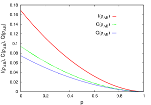
Figure 1: (Color online) Amplitude damping channel: decay of mutual information $I\left(\rho_{AB}\right)$ (solid line), classical correlations $C\left(\rho_{AB}\right)$ (dashed line) and quantum correlations (QD) $Q\left(\rho_{AB}\right)$ (dotted line) as a function of parametrized time $p=1-e^{-\gamma t}$ and $\lambda=0.5$

We next consider the interaction of the chain of qubits, each qubit representing an Ising spin, with an environment. We choose the initial state of the whole system at time $t=0$ to be of the product form, i.e.,

$$\rho(0)=\rho_{s}(0)\otimes\rho_{e}(0)$$ (41)

where the density matrices $\rho_{s}$ and $\rho_{e}$ correspond to the system and environment respectively. We assume that the environment is represented by $L$ independent reservoirs each of which interacts locally with a qubit constituting the Ising chain. The two-qubit reduced density matrix obtained from equation (41) can be written as

$$\rho_{r}(0)=\rho_{rs}(0)\otimes\rho_{re}(0)$$ (42)

where $\rho_{rs}$ and $\rho_{re}$ represent the two-qubit reduced density matrix of the transverse Ising chain and the corresponding reduced density matrix of the two-reservoir environment respectively. The two-qubit reduced density matrix $\rho_{rs}$ is obtained by taking partial trace on $\rho_{s}$ over the states of all the qubits other than the two chosen qubits. Similarly, $\rho_{re}$ is obtained from $\rho_{e}$ by taking a partial trace over the states of all the reservoirs other than the two local reservoirs of the selected qubits. The quantum channel describing the interaction between a qubit and its environment can be of various types: amplitude damping, phase damping, bit-flip, phase-flip, bit-phase-flip etc. maziero1 ; nielsenchuang . Our objective is to investigate the dynamics of the two-qubit classical and quantum correlations (in the form of the QD) under the influence of various quantum channels.

The time evolution of the closed quantum system, comprised of both the system and the environment, is given by

$$\rho_{se}(t)=U(t)\rho_{se}(0)U^{\dagger}(t)$$ (43)

where $U(t)$ is the unitary evolution operator generated by the total Hamiltonian $H$ of the system $\left(U=e^{-iHt/\hbar}\right)$. $H$ is given by $H=H_{s}+H_{e}+H_{se}$ where $H_{s}$ and $H_{e}$ represent the bare system and environment Hamiltonians respectively and $H_{se}$ the Hamiltonian describing the interactions between the system and the environment. The time evolution of the system $s$ subject to the influence of the environment $e$ is obtained by carrying out a partial trace on $\rho_{se}(t)$ (equation (43)) over the environment states, i.e.,

$$\rho_{s}(t)=\mbox{Tr}_{e}\left[U(t)\rho_{se}(0)U^{\dagger}(t)\right]$$ (44)

Let $|e_{k}\rangle$ be an orthogonal basis spanning the finite-dimensional state space of the environment. With the initial state of the whole system given by equation (41),

$$\rho_{s}(t)=\sum_{k}\langle e_{k}|U\left[\rho_{s}(0)\otimes\rho_{e}(0)\right]U^{\dagger}|e_{k}\rangle$$ (45)

Let $\rho_{e}(0)=|e_{0}\rangle\langle e_{0}|$ be the initial state of the environment. Then

$$\rho_{s}(t)=\sum_{k}E_{k}\rho_{s}(0)E_{k}^{\dagger}$$ (46)

where $E_{k}\equiv\langle e_{k}|U|e_{0}\rangle$ is the Kraus operator which acts on the state space of the system only maziero1 ; nielsenchuang . Let $\left\{\phi_{i}\right\}$, $i=1,2,...,d,$ define the basis in the state space of the system $s$. There are then at most $d^{2}$ independent Kraus operators $E_{k}$, $k=0,...,d^{2}-1$ nielsenchuang ; salles . The unitary evolution of $s+e$ is given by the map:

$$|\phi_{1}\rangle|e_{0}\rangle \rightarrow E_{0}|\phi_{1}\rangle|e_{0}\rangle+...+E_{d^{2}-1}|\phi_{1}\rangle|e_{d^{2}-1}\rangle$$

$$|\phi_{2}\rangle|e_{0}\rangle \rightarrow E_{0}|\phi_{2}\rangle|e_{0}\rangle+...+E_{d^{2}-1}|\phi_{2}\rangle|e_{d^{2}-1}\rangle$$

$$\vdots$$

$$|\phi_{d}\rangle|e_{0}\rangle \rightarrow E_{0}|\phi_{d}\rangle|e_{0}\rangle+...+E_{d^{2}-1}|\phi_{d}\rangle|e_{d^{2}-1}\rangle$$ (47)

In compact notation, the map is given by

$$U|\phi_{i}\rangle|e_{0}\rangle\equiv\sum_{k}E_{k}|\phi_{i}\rangle|e_{k}\rangle,\;i=1,2,...,d$$ (48)

In the case of $N$ system parts with each part interacting with a local independent environment, equation (46) becomes

$$\rho_{s}(t)=\sum_{k_{1},..,k_{N}}E_{k_{1}}^{(1)}\otimes..\otimes E_{k_{N}}^{(N)}\rho_{s}(0)E_{k_{1}}^{(1)\dagger}\otimes..\otimes E_{k_{N}}^{(N)\dagger}$$

(49)

where $E_{k_{\alpha}}^{(\alpha)}$ is the $k_{\alpha}$th Kraus operator with the environment acting on system part $\alpha$. The specific form for $\rho_{s}(t)$ arises as the total evolution operator can be written as $U(t)=U_{1}(t)\otimes U_{2}(t)\otimes...\otimes U_{N}(t)$. Following the general formalism of the Kraus operator representation, an initial state, $\rho_{rs}(0)$, of the two-qubit reduced density matrix evolves as werlang1 ; nielsenchuang

$$\rho_{rs}(t)=\sum_{\mu,\nu}E_{\mu,\nu}\rho_{rs}(0)E_{\mu,\nu}^{\dagger}$$ (50)

where the Kraus operators $E_{\mu,\nu}=E_{\mu}\otimes E_{\nu}$ satisfy the completeness relation $\sum_{\mu,\nu}E_{\mu,\nu}E_{\mu,\nu}^{\dagger}=I$ for all $t$. We now briefly describe the various quantum channels considered in the paper and write down the corresponding Kraus operators. A fuller description can be obtained from Refs. werlang1 ; nielsenchuang .

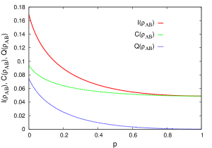
Figure 2: (Color online) Bit-flip channel: decay of mutual information $I\left(\rho_{AB}\right)$ (solid line), classical correlations $C\left(\rho_{AB}\right)$ (dashed line) and quantum correlations (QD) $Q\left(\rho_{AB}\right)$ (dotted line) as a function of parametrized time $p=1-e^{-\gamma t}$ and $\lambda=0.5$

(i) Amplitude Damping Channel.

The channel describes the dissipative interaction between a system and its environment resulting in an exchange of energy between $s$ and $e$ so that $s$ is ultimately in thermal equilibrium with $e$. The $s+e$ time evolution is given by the unitary transformation

$$|0\rangle_{s}|0\rangle_{e} \rightarrow |0\rangle_{s}|0\rangle_{e}$$ (51)

$$|1\rangle_{s}|0\rangle_{e} \rightarrow \sqrt{q}|1\rangle_{s}|0\rangle_{e}+\sqrt{p}|0\rangle_{s}|1\rangle_{e}$$ (52)

where $|0\rangle_{s}$ and $|1\rangle_{s}$ are the ground and excited qubit states and $|0\rangle_{e}$, $|1\rangle_{e}$ denote states of the environment with no excitation (vacuum state) and one excitation respectively. Equation (51) stipulates that there is no dynamic evolution if the system and the environment are in their ground states. Equation (52) states that if the system qubit is in the excited state, the probability to remain in the same state is $q$ and the probability of decaying to the ground state is $p$ $(p+q=1)$. The decay of the qubit state is accompanied by a transition of the environment to a state with one excitation. The qubit states may be two atomic states with the excited state decaying to the ground state by emitting a photon. The environment on acquiring the photon is no longer in the vacuum state. With a knowledge of the map equations (equations (51) and (52)), the Kraus operators for the amplitude damping channel can be written as

$$E_{0}=\left(\begin{array}[]{cc}1&0\\ 0&\sqrt{q}\end{array}\right);\;\;E_{1}=\left(\begin{array}[]{cc}0&\sqrt{p}\\ 0&0\end{array}\right)$$ (57)

where $q=1-p$. The Kraus operators for the two distinct environments (one for each qubit) have identical forms. In the case of Markovian time evolution, $p$ is given by $p=1-e^{-\gamma t}$ with $\gamma$ denoting the decay rate.

(ii) Phase Damping (dephasing) Channel. The channel describes the loss of quantum coherence without loss of energy. The Kraus operators are:

$$E_{0}=\left(\begin{array}[]{cc}1&0\\ 0&\sqrt{q}\end{array}\right);\;\;E_{1}=\left(\begin{array}[]{cc}0&0\\ 0&\sqrt{p}\end{array}\right)$$ (62)

with $q=1-p$ and $p=1-e^{-\gamma t}$.

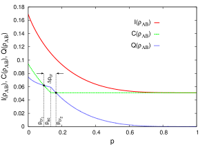
Figure 3: (Color online) Phase-flip channel: decay of mutual information $I\left(\rho_{AB}\right)$ (solid line), classical correlations $C\left(\rho_{AB}\right)$ (dashed line) and quantum correlations (QD) $Q\left(\rho_{AB}\right)$ (dotted line) as a function of parametrized time $p=1-e^{-\gamma t}$ and $\lambda=0.5$. Also, $p_{cr_{1}}=0.0932$, $p_{sc}=0.1347$ and $p_{cr_{2}}=0.1649$

(iii) Bit-flip, phase-flip and bit-phase-flip channels. The channels destroy the information contained in the phase relations without involving an exchange of energy. The Kraus operators are

$$E_{0}=\sqrt{q^{\prime}}\left(\begin{array}[]{cc}1&0\\ 0&1\end{array}\right);\;\;E_{1}=\sqrt{p/2}\sigma_{i}$$ (65)

where $i=x$ for the bit-flip, $i=y$ for the bit-phase-flip and $i=z$ for the phase-flip channel with $q^{\prime}=1-p/2$ and $p=1-e^{-\gamma t}$. The expanded forms of the Kraus operators are:

Bit-flip

$$E_{0} = \left(\begin{array}[]{cc}\sqrt{1-p/2}&0\\ 0&\sqrt{1-p/2}\end{array}\right)$$ (68)

$$E_{1} = \left(\begin{array}[]{cc}0&\sqrt{p/2}\\ \sqrt{p/2}&0\end{array}\right)$$ (71)

Phase-flip

$$E_{0} = \left(\begin{array}[]{cc}\sqrt{1-p/2}&0\\ 0&\sqrt{1-p/2}\end{array}\right)$$ (74)

$$E_{1} = \left(\begin{array}[]{cc}\sqrt{p/2}&0\\ 0&-\sqrt{p/2}\end{array}\right)$$ (77)

Bit-phase-flip

$$E_{0} = \left(\begin{array}[]{cc}\sqrt{1-p/2}&0\\ 0&\sqrt{1-p/2}\end{array}\right)$$ (80)

$$E_{1} = \left(\begin{array}[]{cc}0&-i\sqrt{p/2}\\ i\sqrt{p/2}&0\end{array}\right)$$ (83)

As shown in Ref. nielsenchuang , the phase damping quantum operation is identical to that of the phase-flip channel so that we will consider only one of these, the phase-flip channel, in the following.

For a specific quantum channel, it is now straightforward to calculate the dynamics of the classical and quantum correlations. Equation (50) describes the time evolution of the reduced density matrix of the TIM subjected to the influence of an environment via a quantum channel. The initial state $\rho_{rs}(0)$ has the form given in equation (17) the elements of which are known via the equations (26)-(40). The time-evolved state $\rho_{rs}(t)$ has again the form given in equation (17) with the time dependence occurring in only the off-diagonal elements. With a knowledge of the elements, the mutual information $I(\rho_{AB})$, the QD $Q(\rho_{AB})$ and the classical correlations $C(\rho_{AB})$ can be computed at any time $t$ with the help of the formulae in equations (18)-(24) and equation (2). The results of our calculations for the various quantum channels are described in the next Section.

III Results

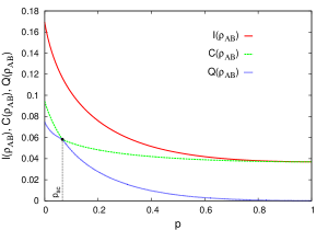
Figure 4: (Color online) Bit-phase-flip channel: decay of mutual information $I\left(\rho_{AB}\right)$ (solid line), classical correlations $C\left(\rho_{AB}\right)$ (dashed line) and quantum correlations (QD) $Q\left(\rho_{AB}\right)$ (dotted line) as a function of parametrized time $p=1-e^{-\gamma t}$ and $\lambda=0.5$. Also, $p_{sc}=0.0666$

In the following, we make the substitution $\rho_{AB}=\rho_{rs}(t)$.

Amplitude Damping Channel. The dynamical evolution of the mutual information $I(\rho_{AB})$, the classical correlations $C(\rho_{AB})$ and the QD $Q(\rho_{AB})$ as a function of the parametrized time $p$ $\left(p=1-e^{-\gamma t}\right)$ is shown in Fig.1 for $\lambda=0.5$. The solid, dashed and dotted lines represent the variations of $I(\rho_{AB})$, $C(\rho_{AB})$ and $Q(\rho_{AB})$ respectively with $p$. All the correlations decay to zero in the asymptotic limit of $t\rightarrow\infty$, i.e., $p\rightarrow 1$. There is further no parametrized time interval or point when the quantum correlation becomes greater than the classical correlation.

Bit-flip Channel. Fig.2 exhibits the dynamical evolution of $I(\rho_{AB})$ (solid line), $C(\rho_{AB})$ (dashed line) and $Q(\rho_{AB})$ (dotted line) as a function of the parametrized times and with $\lambda=0.5$. The quantum correlations disappear completely in the asymptotic limit $p\rightarrow 1$. In the same limit, $I(\rho_{AB})=C(\rho_{AB})$ has a finite value. In the case of both the amplitude damping and bit-flip channels, the same features as observed for $\lambda=0.5$ are obtained for the other values of $\lambda$.

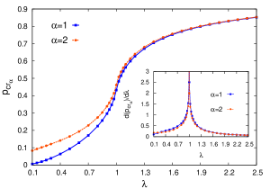
Figure 5: (Color online) Variations of $p_{cr_{1}}$ (solid line) and $p_{cr_{2}}$ (dashed line) with $\lambda$ in the case of the phase-flip channel; (inset) The first derivative of $p_{cr_{1}}$ and $p_{cr_{2}}$ w.r.t $\lambda$ diverges as the QCP $\lambda_{c}=1$ is approached

Phase-flip Channel. In Fig.3, we plot the variations of $I\left(\rho_{AB}\right)$ (solid line), $C\left(\rho_{AB}\right)$ (dashed line) and $Q\left(\rho_{AB}\right)$ (dotted line) versus the parametrized time $p$ with $\lambda=0.5$. There is a sudden change in the decay rates of both $C\left(\rho_{AB}\right)$ and $Q\left(\rho_{AB}\right)$ at $p=p_{sc}$. There are two points, $p=p_{cr_{1}}$ and $p=p_{cr_{2}}$ at which the plots of $C\left(\rho_{AB}\right)$ and $Q\left(\rho_{AB}\right)$ cross each other. The classical correlations remains constant beyond the point $p=p_{sc}$ whereas the QD decays asymptotically to zero. In the parametrized time interval $p_{sc}\leq p\leq 1$, the magnitude of $C\left(\rho_{AB}\right)=\left.I\left(\rho_{AB}\right)\right|_{p=1}$, the mutual information of the completely decohered state $\left(p=1\right)$. In the interval $p_{cr_{1}}<p<p_{cr_{2}}$, the quantum correlations are larger in magnitude than the classical correlations contradicting an earlier conjecture that $C\left(\rho_{AB}\right)\geq Q\left(\rho_{AB}\right)$ in any quantum state maziero2 . At the crossing points, $p_{cr_{1}}$ and $p_{cr_{2}}$, one gets the equality $C\left(\rho_{AB}\right)=Q\left(\rho_{AB}\right)=\frac{I\left(\rho_{AB}\right)}{2}$. Xu et al. xu have recently investigated the dynamics of classical and quantum correlations under decoherence in an all-optical experimental setup. Fig.4 of their paper provides experimental verification of the dynamics displayed in Fig.3.

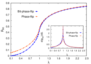
Figure 6: (Color online) Variations of $p_{sc}$ with $\lambda$ for the phase-flip (dashed line) and the bit-phase-flip (solid line) channels; (inset) The first derivative of $p_{sc}$ w.r.t $\lambda$ exhibits a divergence as the QCP $\lambda_{c}=1$ is approached

The sudden change in the decay rates of $Q\left(\rho_{AB}\right)$ and $C\left(\rho_{AB}\right)$ at $p=p_{sc}$ is understood by noting that for $p<p_{sc}$, $Q=Q_{2}$ (equation (22)) and for $p>p_{sc}$, $Q=Q_{1}$ with $C\left(\rho_{AB}\right)$ given by $C\left(\rho_{AB}\right)=I\left(\rho_{AB}\right)-Q\left(\rho_{AB}\right)$. At the crossing points $p_{cr_{1}}$ and $p_{cr_{2}}$, $Q\left(\rho_{AB}\right)=C\left(\rho_{AB}\right)$ so that $p_{cr_{1}}$ and $p_{cr_{2}}$ are the solutions of the equations $Q_{2}=\left(I\left(\rho_{AB}\right)-Q_{2}\right)$ and $Q_{1}=\left(I\left(\rho_{AB}\right)-Q_{1}\right)$ respectively. The constancy of $C\left(\rho_{AB}\right)$ for values of $p>p_{sc}$ is explained by the fact that $Q=Q_{1}$ in this regime. From equations (1), (2) and (23),

$$C\left(\rho_{AB}\right) = S\left(\rho_{A}\right)+a\log_{2}\frac{a}{a+b}+b\log_{2}\frac{b}{a+b}$$ (84)

$$+d\log_{2}\frac{d}{d+b}+b\log_{2}\frac{b}{d+b}$$

As already pointed out, the time-evolved state $\rho_{rs}(t)$ has the form given in equation (17) with the diagonal elements $a$, $b$ and $d$ being independent of time. From (19) and (21), $S\left(\rho_{B}\right)$ is thus independent of time. The other terms in equation (84) are also independent of time since they involve only the elements $a$, $b$ and $d$.

Bit-phase-flip Channel. Fig.4 shows the plots of $I\left(\rho_{AB}\right)$ (solid line), $C\left(\rho_{AB}\right)$ (dashed line) and $Q\left(\rho_{AB}\right)$ (dotted line) as a function of $p$. Again, there is a sudden change, as in the case of the phase flip channel, in the decay dynamics of $C\left(\rho_{AB}\right)$ and $Q\left(\rho_{AB}\right)$ at $p=p_{sc}$ but in this case the two plots do not cross each other but touch at a single point $p=p_{sc}$.

The dynamical features for the different quantum channels have been reported earlier maziero2 for the class of states with $a=d$ in the reduced density matrix of equation (17), i.e., $c_{4}=0$ in equation (19). In our study, the reduced density matrix has the form shown in equation (17) with $a\neq d$, i.e., $c_{4}\neq 0$. The form corresponds to that of the two-qubit reduced density matrix obtained from the ground state of the TIM in 1d. In this case each quantum channel is distinguished by a specific type of dynamics. In Ref. maziero2 , the parameters $c_{1}$, $c_{2}$ and $c_{3}$ are free and different types of dynamics occur in different parameter regions corresponding to the same quantum channel.

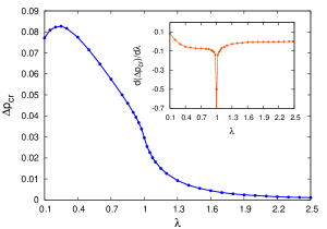
Figure 7: (Color online) Variation of $\Delta p_{cr}=p_{cr_{2}}-p_{cr_{1}}$ with $\lambda$; (inset) The first derivative of $\Delta p_{cr}$ w.r.t $\lambda$ diverges in the negative direction as the QCP $\lambda_{c}=1$ is approached

We now present some totally new results which have not been reported earlier. Fig.5 shows plots of $p_{cr_{1}}$ (solid line) and $p_{cr_{2}}$ (dashed line) versus $\lambda$, the parameter appearing in the TIM Hamiltonian (equation (25)), in the case of the phase-flip channel. The inset of the Figure shows that the first derivative of $p_{cr_{1}}$ and $p_{cr_{2}}$ (both of which depend on $\lambda$) w.r.t. the parameter $\lambda$ diverges as the QCP $\lambda_{c}=1$ is approached. The observation identifies a quantity which provides the signature of a QPT occurring in a system subjected to decoherence under Markovian time evolution. Fig.6 shows a variation of $p_{sc}$ with $\lambda$ for the phase-flip (dashed line) and the bit-phase-flip (solid line) channels. Again, the inset shows that the first derivative of $p_{sc}$ w.r.t $\lambda$ diverges as the QCP $\lambda_{c}=1$ is approached. Fig.7 exhibits the plot of $\Delta p_{cr}=p_{cr_{2}}-p_{cr_{1}}$ versus $\lambda$ in the case of the phase-flip channel. The inset shows that $\frac{d\left(\Delta p_{cr}\right)}{d\lambda}$ diverges in the negative direction as the QCP $\lambda_{c}=1$ is approached. We remind ourselves that when $p$ falls in the interval $\Delta p_{cr}$, the quantum correlations $Q\left(\rho_{AB}\right)$ are larger in magnitude than the classical correlations $C\left(\rho_{AB}\right)$. Fig.7 is an outcome of the results of Fig.5 as $\Delta p_{cr}=p_{cr_{2}}-p_{cr_{1}}$. In summary, the first derivative of any one of the quantities $p_{cr_{1}}$, $p_{cr_{2}}$, $p_{sc}$ and $\Delta p_{cr}$ w.r.t $\lambda$ signals a quantum critical point transition. The quantities correspond to states in which the quantum correlations are either equal to or greater than the classical correlations. At $p=p_{cr_{1}}$ and $p=p_{cr_{2}}$, $Q\left(\rho_{AB}\right)=C\left(\rho_{AB}\right)=I\left(\rho_{AB}\right)/2$ which is characteristic of pure states with $Q\left(\rho_{AB}\right)$ being equal to the entropy of entanglement henderson ; winter . The amplitude damping and bit-flip channels do not have these features. The appearance of singularities in the first derivatives of the quantities $p_{cr_{1}}$, $p_{cr_{2}}$, $p_{sc}$ and $\Delta p_{cr}$ with respect to the tuning parameter as the quantum critical point is approached can be explained by the fact that these quantities depend on two-spin correlation functions which exhibit a similar property close to the critical point. The non-trivial aspect arises from the identification of appropriate quantities associated with the dynamics of correlations which provide clear signatures of QPTs.

IV Concluding remarks

The TIM in 1d is a prototypical example of a quantum system exhibiting a QPT. The many body ground state has both classical and quantum correlations. The QD provides a quantitative measure of the quantum correlations in a two-qubit state. In this paper, we consider a two-qubit state described by the reduced density matrix obtained from the ground state of the TIM in 1d. The two-qubit state undergoes Markovian time evolution, described by the Kraus operator formalism, due to the local interactions of the qubits with independent environments. We consider the quantum channels, representing the interactions, to be of four types: amplitude damping, bit-flip, phase-flip and bit-phase-flip. The dynamics of the classical and quantum correlations exhibit distinctive features for each quantum channel. These features have been reported in an earlier study maziero2 for a different class of initial states. In our study, we have not found evidence of another type of dynamical behaviour mentioned in maziero2 , namely, that the classical correlations, $C\left(\rho_{AB}\right)$, are independent of time throughout the parametrized time interval $p$ whereas the QD, $Q\left(\rho_{AB}\right)$, decreases monotonically and becomes zero in the asymptotic limit $p\rightarrow 1$. The time evolution of the reduced density matrix of the TIM in 1d further does not exhibit the interesting dynamical behaviour described in mazzola , namely, the existence of intervals of parametrized time when $C\left(\rho_{AB}\right)$ and $Q\left(\rho_{AB}\right)$ are individually frozen. The most significant result of our study is the identification of quantities associated with the dynamics of the classical and quantum correlations which diverge as the QCP of the TIM in 1d, $\lambda_{c}=1$, is approached thus providing a distinctive signature of a QPT from a different perspective. The generalization of the result to other model systems exhibiting QPTs will certainly be of significant interest. In the present study, we have restricted our attention to Markovian time evolution. The more general case of non-Markovian time evolution can be investigated only after the appropriate calculational scheme for a system of interacting qubits is developed pal .

References

- (1) L. Amico, R. Fazio, A. Osterloh, V. Vedral, Rev. Mod. Phys. 80, 517 (2008)
- (2) M. Lewenstein, A. Sanpera, V. Ahufinger, B. Damski, A. Sen, U. Sen, Adv. Phys. 56, 243 (2007)
- (3) R. Horodecki, P. Horodecki, M. Horodecki, K. Horodecki, Rev. Mod. Phys. 81, 865 (2009)
- (4) H. Ollivier, W. H. Zurek, Phys. Rev. Lett. 88, 017901 (2001)
- (5) L. Henderson, V. Vedral, J. Phys. A: Math. Gen. 34, 6899 (2001)
- (6) W. H. Zurek, Rev. Mod. Phys. 75, 715 (2003)
- (7) A. Datta, A. Shaji, C. M. Caves, Phys. Rev. Lett. 100, 050502 (2008)
- (8) B. P. Lanyon, M. Bartieri, M. P. Almeida, A. G. White, Phys. Rev. Lett. 101, 200501 (2008)
- (9) S. Luo, Phys. Rev. A 77, 042303 (2008)
- (10) M. S. Sarandy, Phys. Rev. A 80, 022108 (2009)
- (11) M. Ali, A. R. P. Rau, G. Alber, Phys. Rev. A 81, 042105 (2010)
- (12) F. F. Fanchini, T. Werlang, C. A. Brasil, L. G. E. Arruda, A. O. Caldeira, Phys. Rev. A 81, 052107 (2010)
- (13) J. Maziero, T. Werlang, F. F. Fanchini, L. C. Céleri, R. M. Serra, Phys. Rev. A 81, 022116 (2010)
- (14) M. P. Almeida et al., Science 316, 579 (2007)
- (15) T. Werlang, S. Souza, F. F. Fanchini, C. Villas Boas, Phys. Rev. A 80, 024103 (2009)
- (16) J. Maziero, L. C. Céleri, R. M. Serra, V. Vedral, Phys. Rev. A 80, 044102 (2009)
- (17) L. Mazzola, J. Piilo, S. Maniscalco, Phys. Rev. Lett. 104, 200401 (2010)
- (18) A. K. Pal, I. Bose, J. Phys. B: At. Mol. Opt. Phys. 44, 045101 (2011)
- (19) A. Ferraro, L. Aolita, D. Cavalcanti, F. M. Cucchietti, A. Acin, Phys. Rev. A 81, 052318 (2010)
- (20) J.-S. Xu, X.-Y. Xu, C.-F. Li, C.-J. Zhang, X.-B. Zou, G.-C. Guo, Nat. Commun. 1, 7 (2010)
- (21) R. Auccaise et al., Phys. Rev. Lett. 107, 140403 (2011)
- (22) A. Dutta, U. Divakaran, D. Sen, B. K. Chakrabarti, T. F. Rosenbaum, G. Aeppli, arXiv:1012.0653v1 [cond-mat.stat-mech] (2011), to appear in Rev. Mod. Phys.
- (23) J. Osborne, M. A. Nielsen, Phys. Rev. A 66, 032110 (2002)
- (24) A. Osterloh, L. Amico, G. Falci, R. Fazio, Nature 416, 608 (2002)
- (25) R. Dillenschneider, Phys. Rev. B 78, 224413 (2008)
- (26) T. Werlang, G. A. P. Ribeiro, G. Rigolin, Phys. Rev. A 83, 062334 (2011)
- (27) O. F. Syljuåsen, Phys. Rev. A 68, 060301 (R) (2003)
- (28) E. Barouch, B. M. McCoy, Phys. Rev. A 3, 786 (1971)
- (29) P. Pfeuty, Ann. Phys. 57, 79 (1970)
- (30) M. A. Nielsen, I. L. Chuang in Quantum Computation and Quantum Information (Cambridge University Press, Cambridge, England, 2000)
- (31) A. Salles et. al., Phys. Rev. A 78, 022322 (2008)
- (32) B. Groisman, S. Popescu, A. Winter, Phys. Rev. A 72, 032317 (2005)