Natural frequencies of cracked functionally graded material plates by the extended finite element method

Abstract

In this paper, the linear free flexural vibration of cracked functionally graded material plates is studied using the extended finite element method. A 4-noded quadrilateral plate bending element based on field and edge consistency requirement with 20 degrees of freedom per element is used for this study. The natural frequencies and mode shapes of simply supported and clamped square and rectangular plates are computed as a function of gradient index, crack length, crack orientation and crack location. The effect of thickness and influence of multiple cracks is also studied.

1 Introduction

Engineered materials such as laminated composites are widely used in automotive and aerospace industry due to their excellent strength-to and stiffness-to-weight ratios and their possibility of tailoring their properties in optimizing their structural response. But due to sudden change in material properties between the layers in laminated composites, these materials suffer from premature failure or by the decay of stiffness characteristics because of delaminations and chemically unstable matrix and lamina adhesives. The emergence of functionally graded materials (FGMs) [1, 2] has revolutionized the aerospace and aerocraft industry. The FGMs used initially as thermal barrier materials for aerospace structural applications and fusion reactors are now developed for general use as structural components in high temperature environments. FGMs are manufactured by combining metals and ceramics. These materials are inhomogeneous, in the sense that the material properties vary smoothly and continuously in one or more directions. FGMs combine the best properties of metals and ceramics and are strongly considered as a potential structural material candidates for certain class of aerospace structures exposed to a high temperature environment.

It is seen from the literature that the amount of work carried out on the vibration characteristics of FGMs is considerable [3, 4, 5, 6, 7, 8, 9]. He et al., [5] presented finite element formulation based on thin plate theory for the vibration control of FGM plate with integrated piezoelectric sensors and actuators under mechanical load whereas Liew et al., [6]have analyzed the active vibration control of plate subjected to a thermal gradient using shear deformation theory. Ng et al., [7] have investigated the parametric resonance of plates based on Hamilton‘s principle and the assumed mode technique. Yang and Shen [10] have analyzed the dynamic response of thin FGM plates subjected to impulsive loads using Galerkin procedure coupled with modal superposition method whereas, by neglecting the heat conduction effect, such plates and panels in thermal environments have been examined based on shear deformation with temperature dependent material properties in [8]. Qian et al., [11] studied the static deformation and vibration of FGM plates based on higher-order shear deformation theory using meshless local Petrov-Galerkin method. Matsunaga [4] presented analytical solutions for simply supported rectangular FGM plates based on second-order shear deformation plates. Vel and Batra [3] proposed three-dimensional solutions for vibrations of simply supported rectangular plates. Reddy [12] presented a finite element solution for the dynamic analysis of a FGM plate and Ferreira et al., [9] peformed dynamic analysis of FGM plate based on higher order shear and normal deformable plate theory using the meshless local Petrov-Galerkin method. Akbari et al., [13] studied two-dimensional wave propagation in functionally graded solids using the meshless local Petrov-Galerkin method. The above list is no way comprehensive and interested readers are referred to the literature.

FGM plates or in general plate structures, may develop flaws during manufacturing or after they have been subjected to large cyclic loading. Hence it is important to understand the dynamic response of a FGM plate with an internal flaw. It is known that cracks or local defects affect the dynamic response of a structural member. This is because, the presence of the crack introduces local flexibility and anisotropy. Moreover the crack will open and close depending on the vibration amplitude. The vibration of cracked plates was studied as early as 1969 by Lynn and Kumbasar [14] who used a Green’s function approach. Later, in 1972, Stahl and Keer [15] studied the vibration of cracked rectangular plates using elasticity methods. The other numerical methods that are used to study the dynamic response and instability of plates with cracks or local defects are: (1) Finite fourier series transform [16]; (2) Rayleigh-Ritz Method [17]; (3) harmonic balance method [18]; and (4) finite element method [19, 20]. Recently,  [21] proposed solutions for the virbations of side-cracked FGM thick plates based on Reddy third-order shear deformation theory using Ritz technique. Kitipornchai et al., [22] studied nonlinear vibration of edge cracked functionally graded Timoshenko beams using Ritz method. Yang et al., [23] studied the nonlinear dynamic response of a functionally graded plate with a through-width crack based on Reddy’s third-order shear deformation theory using a Galerkin method.

In this paper, we apply the extended finite element method (XFEM) to study the free flexural vibrations of cracked FGM plates based on first order shear deformation theory. We carry out a parametric study on the influence of gradient index, crack location, crack length, crack orientation and thickness on the natural frequencies of FGM plates using the 4-noded shear flexible element based on field and edge consistency approach [24]. The effect of boundary conditions and multiple cracks is also studied. Earlier, the XFEM has been applied to study the vibration of cracked isotropic plates [25, 26, 27]. Their study focussed on center and edge cracks with simply supported and clamped boundary conditions.

The paper is organized as follows, the next section will give an introduction to FGM and a brief overview of Reissner-Mindlin plate theory. Section 3 illustrates the basic idea of XFEM as applicable to plates. Section 4 presents results for the free flexural vibration of cracked plates under different boundary conditions and aspect ratios, followed by concluding remarks in the last section.

2 Theoretical Formulation

2.1 Functionally Graded Material

A functionally graded material (FGM) rectangular plate (length $a$, width $b$ and thickness $h$), made by mixing two distinct material phases: a metal and ceramic is considered with coordinates $x,y$ along the in-plane directions and $z$ along the thickness direction (see Figure (2)). The material on the top surface $(z=h/2)$ of the plate is ceramic and is graded to metal at the bottom surface of the plate $(z=-h/2)$ by a power law distribution. The homogenized material properties are computed using the Mori-Tanaka Scheme [28, 29].

Estimation of mechanical and thermal properties

Based on the Mori-Tanaka homogenization method, the effective bulk modulus $K$ and shear modulus $G$ of the FGM are evaluated as [28, 29, 30, 11]

$${K-K_{m}\over K_{c}-K_{m}} = {V_{c}\over 1+(1-V_{c}){3(K_{c}-K_{m})\over 3K_{m}+4G_{m}}}$$

$${G-G_{m}\over G_{c}-G_{m}} = {V_{c}\over 1+(1-V_{c}){(G_{c}-G_{m})\over G_{m}+f_{1}}}$$ (1)

where

$$f_{1}={G_{m}(9K_{m}+8G_{m})\over 6(K_{m}+2G_{m})}$$ (2)

Here, $V_{i}~{}(i=c,m)$ is the volume fraction of the phase material. The subscripts $c$ and $m$ refer to the ceramic and metal phases, respectively. The volume fractions of the ceramic and metal phases are related by $V_{c}+V_{m}=1$, and $V_{c}$ is expressed as

$$V_{c}(z)=\left({2z+h\over 2h}\right)^{n},\hskip 5.69046ptn\geq 0$$ (3)

where $n$ in Equation (3) is the volume fraction exponent, also referred to as the gradient index. Figure (1) shows the variation of the volume fractions of ceramic and metal, respectively, in the thickness direction $z$ for the FGM plate. The top surface is ceramic rich and the bottom surface is metal rich.

Figure 1: Through thickness variation of volume fraction

The effective Young’s modulus $E$ and Poisson’s ratio $\nu$ can be computed from the following expressions:

$$E={9KG\over 3K+G}$$

$$\nu={3K-2G\over 2(3K+G)}$$ (4)

The effective mass density $\rho$ is given by the rule of mixtures as [3]

$$\rho=\rho_{c}V_{c}+\rho_{m}V_{m}$$ (5)

The material properties $P$ that are temperature dependent can be written as [31]

$$P=P_{o}(P_{-1}T^{-1}+1+P_{1}T+P_{2}T^{2}+P_{3}T^{3}),$$ (6)

where $P_{o},P_{-1},P_{1},P_{2},P_{3}$ are the coefficients of temperature $T$ and are unique to each constituent material phase.

2.2 Plate formulation

Using the Mindlin formulation, the displacements $u,v,w$ at a point $(x,y,z)$ in the plate (see Figure (2)) from the medium surface are expressed as functions of the mid-plane displacements $u_{o},v_{o},w_{o}$ and independent rotations $\theta_{x},\theta_{y}$ of the normal in $yz$ and $xz$ planes, respectively, as

Figure 2: Co-ordinate system of a rectangular FGM plate.

$$u(x,y,z,t) = u_{o}(x,y,t)+z\theta_{x}(x,y,t)$$

$$v(x,y,z,t) = v_{o}(x,y,t)+z\theta_{y}(x,y,t)$$

$$w(x,y,z,t) = w_{o}(x,y,t)$$ (7)

where $t$ is the time. The strains in terms of mid-plane deformation can be written as

$$\boldsymbol{\varepsilon}=\left\{\begin{array}[]{c}\boldsymbol{\varepsilon}_{p}\\ 0\end{array}\right\}+\left\{\begin{array}[]{c}z\boldsymbol{\varepsilon}_{b}\\ \boldsymbol{\varepsilon}_{s}\end{array}\right\}$$ (8)

The midplane strains $\boldsymbol{\varepsilon}_{p}$, bending strain $\boldsymbol{\varepsilon}_{b}$, shear strain $\boldsymbol{\varepsilon}_{s}$ in Equation (8) are written as

$$\boldsymbol{\varepsilon}_{p}=\left\{\begin{array}[]{c}u_{o,x}\\ v_{o,y}\\ u_{o,y}+v_{o,x}\end{array}\right\},\hskip 28.45274pt\boldsymbol{\varepsilon}_{b}=\left\{\begin{array}[]{c}\theta_{x,x}\\ \theta_{y,y}\\ \theta_{x,y}+\theta_{y,x}\end{array}\right\}$$ (15)

$$\boldsymbol{\varepsilon}_{s}=\left\{\begin{array}[]{c}\theta_{x}+w_{o,x}\\ \theta_{y}+w_{o,y}\end{array}\right\},\hskip 28.45274pt$$ (18)

where the subscript ‘comma’ represents the partial derivative with respect to the spatial coordinate succeeding it. The membrane stress resultants $\mathbf{N}$ and the bending stress resultants $\mathbf{M}$ can be related to the membrane strains, $\boldsymbol{\varepsilon}_{p}$ and bending strains $\boldsymbol{\varepsilon}_{b}$ through the following constitutive relations

$$\mathbf{N} = \left\{\begin{array}[]{c}N_{xx}\\ N_{yy}\\ N_{xy}\end{array}\right\}=\mathbf{A}\boldsymbol{\varepsilon}_{p}+\mathbf{B}\boldsymbol{\varepsilon}_{b}$$ (22)

$$\mathbf{M} = \left\{\begin{array}[]{c}M_{xx}\\ M_{yy}\\ M_{xy}\end{array}\right\}=\mathbf{B}\boldsymbol{\varepsilon}_{p}+\mathbf{D_{b}}\boldsymbol{\varepsilon}_{b}$$ (26)

where the matrices $\mathbf{A}=A_{ij},\mathbf{B}=B_{ij}$ and $\mathbf{D_{b}}=D_{ij};(i,j=1,2,6)$ are the extensional, bending-extensional coupling and bending stiffness coefficients and are defined as

$$\left\{A_{ij},~{}B_{ij},~{}D_{ij}\right\}=\int_{-h/2}^{h/2}\overline{Q}_{ij}\left\{1,~{}z,~{}z^{2}\right\}~{}dz$$ (27)

Similarly, the transverse shear force $Q=\{Q_{xz},Q_{yz}\}$ is related to the transverse shear strains $\boldsymbol{\varepsilon}_{s}$ through the following equation

$$Q_{ij}=E_{ij}\boldsymbol{\varepsilon}_{s}$$ (28)

where $E_{ij}=\int_{-h/2}^{h/2}\overline{Q}\upsilon_{i}\upsilon_{j}~{}dz;~{}(i,j=4,5)$ is the transverse shear stiffness coefficient, $\upsilon_{i},\upsilon_{j}$ is the transverse shear coefficient for non-uniform shear strain distribution through the plate thickness. The stiffness coefficients $\overline{Q}_{ij}$ are defined as

$$\overline{Q}_{11}=\overline{Q}_{22}={E(z,T)\over 1-\nu^{2}};\hskip 28.45274pt\overline{Q}_{12}={\nu E(z,T)\over 1-\nu^{2}};\hskip 28.45274pt\overline{Q}_{16}=\overline{Q}_{26}=0$$

$$\overline{Q}_{44}=\overline{Q}_{55}=\overline{Q}_{66}={E(z,T)\over 2(1+\nu)}$$ (29)

where the modulus of elasticity $E(z,T)$ and Poisson’s ratio $\nu$ are given by Equation (4). The strain energy function $U$ is given by

$$U(\boldsymbol{\delta})={1\over 2}\int_{\Omega}\left\{\boldsymbol{\varepsilon}_{p}^{\textup{T}}\mathbf{A}\boldsymbol{\varepsilon}_{p}+\boldsymbol{\varepsilon}_{p}^{\rm T}\mathbf{B}\boldsymbol{\varepsilon}_{b}+\boldsymbol{\varepsilon}_{b}^{\textup{T}}\mathbf{B}\boldsymbol{\varepsilon}_{p}+\boldsymbol{\varepsilon}_{b}^{\textup{T}}\mathbf{D}\boldsymbol{\varepsilon}_{b}+\boldsymbol{\varepsilon}_{s}^{\textup{T}}\mathbf{E}\boldsymbol{\varepsilon}_{s}\right\}~{}d\Omega$$ (30)

where $\boldsymbol{\delta}=\{u,v,w,\theta_{x},\theta_{y}\}$ is the vector of the degree of freedom associated to the displacement field in a finite element discretization. Following the procedure given in [32], the strain energy function $U$ given in Equation (30) can be rewritten as

$$U(\boldsymbol{\delta})={1\over 2}\boldsymbol{\delta}^{\textup{T}}\mathbf{K}\boldsymbol{\delta}$$ (31)

where $\mathbf{K}$ is the linear stiffness matrix. The kinetic energy of the plate is given by

$$T(\boldsymbol{\delta})={1\over 2}\int_{\Omega}\left\{I_{o}(\dot{u}_{o}^{2}+\dot{v}_{o}^{2}+\dot{w}_{o}^{2})+I_{1}(\dot{\theta}_{x}^{2}+\dot{\theta}_{y}^{2})\right\}~{}d\Omega$$ (32)

where $I_{o}=\int_{-h/2}^{h/2}\rho(z)~{}dz,~{}I_{1}=\int_{-h/2}^{h/2}z^{2}\rho(z)~{}dz$ and $\rho(z)$ is the mass density that varies through the thickness of the plate given by Equation (5). Substituting Equation (31) - (32) in Lagrange’s equations of motion, the following governing equation is obtained

$$\mathbf{M}\ddot{\boldsymbol{\delta}}+\mathbf{K}\boldsymbol{\delta}=\mathbf{0}$$ (33)

where $\mathbf{M}$ is the consistent mass matrix. After substituting the characteristic of the time function [33] $\ddot{\boldsymbol{\delta}}=-\omega^{2}\boldsymbol{\delta}$, the following algebraic equation is obtained

$$\left(\mathbf{K}-\omega^{2}\mathbf{M}\right)\boldsymbol{\delta}=\mathbf{0}$$ (34)

where $\mathbf{K}$ is the stiffness matrix, $\omega$ is the natural frequency.

3 Overview of the extended finite element method

In this section, we give a brief overview of the XFEM for plates. By exploiting the idea of partition of unity noted by Babuška et al., [34], Belytschko’s group [35] introduced the XFEM to solve linear elastic fracture mechanics problems. The conventional expansion of the displacement field using a polynomial basis fails to capture the local behavior of the problem (e.g., steep stress gradients, material discontinuity). Hence, new functions are added to the conventional set of basis functions that contain information regarding the localized behavior. In general, the field variables are approximated by [35, 36, 37, 38, 39, 40]:

$$\mathbf{u}^{h}(\mathbf{x})=\sum\limits_{i\in\mathcal{N}^{\rm{fem}}}{N_{i}}(\mathbf{x})\mathbf{q}_{i}+\textup{enrichment functions}$$ (35)

where $N_{i}(\mathbf{x})$ are standard finite element shape functions, $\mathbf{q}_{I}$ are nodal variables associated with node $I$. In the following, we briefly describe the standard discretization of a plate using the field consistent Q4 plate element. The enriched field consistent Q4 element is then described. And finally, the discretized equations for the eigenvalue problem is given. In this section, only the essential details are given, interested readers are referred to recent review papers on XFEM [41, 42]. A review on the implementation of the extended finite element is given in [43] and a detailed description of the state of the art on the simulation of cracks by partition of unity enriched methods is given in [44].

3.1 Element Description

The plate element employed here is a $\mathcal{C}^{0}$ continuous shear flexible field consistent element with five degrees of freedom $(u_{o},v_{o},w_{o},\theta_{x},\theta_{y})$ at four nodes in an 4-noded quadrilateral (QUAD-4) element. If the interpolation functions for QUAD-4 are used directly to interpolate the five variables $(u_{o},v_{o},w_{o},\theta_{x},\theta_{y})$ in deriving the shear strains and membrane strains, the element will lock and show oscillations in the shear and membrane stresses. The field consistency requires that the transverse shear strains and membrane strains must be interpolated in a consistent manner. Thus, the $\theta_{x}$ and $\theta_{y}$ terms in the expressions for shear strain $\boldsymbol{\varepsilon}_{s}$ have to be consistent with the derivative of the field functions, $w_{o,x}$ and $w_{o,y}$. This is achieved by using field redistributed substitute shape functions to interpolate those specific terms, which must be consistent as described in [24, 33]. This element is free from locking and has good convergence properties. For complete description of the element, interested readers are referred to the literature [24, 33], where the element behavior is discussed in great detail. Since the element is based on the field consistency approach, exact integration is applied for calculating various strain energy terms.

3.2 Enriched Q4 element

Consider a mesh of field consistent Q4 elements and an independent crack geometry as shown in Figure (3). The following enriched approximation proposed by Dolbow et al., [45] for the plate displacements and the section rotations are used:

Figure 3: A typical FE mesh with an arbitrary crack. ‘Squared’ nodes are enriched with the heaviside function and ‘circled’ nodes with the near tip functions, which allows representing cracks independent of the background mesh.

$$\begin{split}(u^{h},v^{h},w^{h})\left(\mathbf{x}\right)=\sum_{i\in\mathcal{N}^{\rm{fem}}}\phi_{i}(\mathbf{x})(u_{i},v_{i},w_{i})+\sum_{j\in\mathcal{N}^{\rm{c}}}\phi_{j}(\mathbf{x})H(\mathbf{x})(b_{j}^{u},b_{j}^{v},b_{j}^{w})+\\ \sum_{k\in\mathcal{N}^{\rm{f}}}\phi_{k}(\mathbf{x})\left(\sum_{l=1}^{4}(c_{kl}^{u},c_{kl}^{v},c_{kl}^{w})G_{l}(r,\theta)\right)\end{split}$$ (36)

The section rotations in the shear terms are approximated by

$$\begin{split}(\theta_{x}^{h},\theta_{y}^{h})\left(\mathbf{x}\right)=\sum_{i\in\mathcal{N}^{\rm{fem}}}\tilde{\phi}_{i}(\mathbf{x})(\theta_{x_{i}},\theta_{y_{i}})+\sum_{j\in\mathcal{N}^{\rm{c}}}\tilde{\phi}_{j}(\mathbf{x})H(\mathbf{x})(b_{j}^{\theta_{x}},b_{j}^{\theta_{y}})+\\ \sum_{k\in\mathcal{N}^{\rm{f}}}\tilde{\phi}_{k}(\mathbf{x})\left(\sum_{l=1}^{4}(c_{kl}^{\theta_{x}},c_{kl}^{\theta_{y}})F_{l}(r,\theta)\right).\end{split}$$ (37)

In Equations (36) and (37), $(u_{i},v_{i},w_{i},\theta_{x_{i}},\theta_{y_{i}})$ are the nodal unknown vectors associated with the continuous part of the finite element solution, $b_{j}$ is the nodal enriched degree of freedom vector associated with the Heaviside (discontinuous) function, and $c_{kl}$ is the nodal enriched degree of freedom vector associated with the elastic asymptotic crack-tip functions. The asymptotic functions, $G_{l}$ and $F_{l}$ in Equations (36) and (37) are given by ([45]):

$$G_{l}(r,\theta)\equiv\left\{\sqrt[3]{r}\sin\left(\frac{\theta}{2}\right),\sqrt[3]{r}\cos\left(\frac{\theta}{2}\right),\sqrt[3]{r}\sin\left(\frac{3\theta}{2}\right),\sqrt[3]{r}\cos\left(\frac{3\theta}{2}\right)\right\},$$ (38a)

$$F_{l}(r,\theta)\equiv\sqrt{r}\left\{\sin\left(\frac{\theta}{2}\right),\cos\left(\frac{\theta}{2}\right),\sin\left(\frac{\theta}{2}\right)\sin\left(\theta\right),\cos\left(\frac{\theta}{2}\right)\sin\left(\theta\right)\right\}.$$ (38b)

Here $(r,\theta)$ are polar coordinates in the local coordinate system with the origin at the crack tip. The functions described here to recover the singular fields around the crack tip were originally proposed for isotropic plates [45]. As we are interested in the global behavior of the cracked FGM plate, we propose to use the same enrichment functions. The role of these enrichment functions is to aid in representing the discontinuous surface independent of the mesh.

In Equations (36) and (37), $\mathcal{N}^{\rm{fem}}$ is the set of all nodes in the mesh; $\mathcal{N}^{\rm{c}}$ is the set of nodes whose shape function support is cut by the crack interior (squared nodes in Figure (3)) and $\mathcal{N}^{\rm{f}}$ is the set of nodes whose shape function support is cut by the crack tip (circled nodes in Figure (3)). For any node in $\mathcal{N}^{\rm{f}}$, the support of the nodal shape function is fully cut into two disjoint pieces by the crack. If for a certain node $n_{i}$, one of the two pieces is very small compared to the other, then the generalized Heaviside function used for the enrichment is almost a constant over the support, leading to an ill-conditioned matrix [46]. Therefore, in this case, the node $n_{i}$ is removed from the set $\mathcal{N}^{\rm{c}}$. The area-criterion for the nodal inclusion in $\mathcal{N}^{\rm{c}}$ is as follows: let the area above the crack is $A^{ab}_{\omega}$ and the area below the crack is $A^{be}_{\omega}$ and $A_{\omega}=A^{ab}_{\omega}+A^{be}_{\omega}$. If either of the two ratios, $A^{ab}_{\omega}/A_{\omega}$ or $A^{be}_{\omega}/A_{\omega}$ is below a prescribed tolerance, the node is removed from the set $\mathcal{N}^{\rm{c}}$. A tolerance of 10^-4 is used in the computations.

3.3 Discretized equations for enriched Q4 plate element

Now, applying the displacement field approximated by Equations (36) - (37) in Equation (30) and Equation (32), one gets the modified Lagrange’s equations of motion in discretized form as:

$$\left(\tilde{\mathbf{K}}-\omega^{2}\tilde{\mathbf{M}}\right)\boldsymbol{\delta}=\mathbf{0},$$ (39)

where the element stiffness matrix is given by:

$$\tilde{\mathbf{K}}^{e}=\left[\begin{array}[]{*{20}c}\tilde{\mathbf{K}}_{uu}^{e}&\tilde{\mathbf{K}}_{ua}^{e}\\ \tilde{\mathbf{K}}_{au}^{e}&\tilde{\mathbf{K}}_{aa}^{e}\end{array}\right]=\int_{\Omega^{e}}\left[\begin{array}[]{*{20}c}\mathbf{B}_{std}^{T}\mathbf{D}\mathbf{B}_{std}&\mathbf{B}_{std}^{T}\mathbf{D}\mathbf{B}_{enr}\\ \mathbf{B}_{enr}^{T}\mathbf{D}\mathbf{B}_{std}&\mathbf{B}_{enr}^{T}\mathbf{D}\mathbf{B}_{enr}\end{array}\right]~{}d\Omega_{e},$$ (40)

where $\mathbf{B}_{std}$ and $\mathbf{B}_{enr}$ are the standard and enriched part of the strain-displacement matrix, respectively and $\mathbf{D}$ is the material matrix. The element mass matrix is given by:

$$\tilde{\mathbf{M}}^{e}=\left[\begin{array}[]{*{20}c}\tilde{\mathbf{M}}_{uu}^{e}&\tilde{\mathbf{M}}_{ua}^{e}\\ \tilde{\mathbf{M}}_{au}^{e}&\tilde{\mathbf{M}}_{aa}^{e}\end{array}\right]=\int_{\Omega^{e}}\left[\begin{array}[]{*{20}c}\mathbf{N}_{std}^{T}~{}\rho\mathbf{N}_{std}&\mathbf{N}_{std}^{T}~{}\rho\mathbf{N}_{enr}\\ \mathbf{N}_{enr}^{T}~{}\rho\mathbf{N}_{std}&\mathbf{N}_{enr}^{T}~{}\rho\mathbf{N}_{enr}\end{array}\right]~{}d\Omega_{e}.$$ (41)

where in deriving the above element mass matrix, the plate displacements and the section rotations given by Equations (36) - (37) are used. In solving for the eigenvalues, the QR algorithm, based on the QR decomposition is used [47].

4 Numerical results

In this section, we present the natural frequencies of a cracked functionally graded material plates using the extended Q4 formulation. We consider both square and rectangular plates with simply supported, cantilevered and clamped boundary conditions. In all cases, we present the non dimensionalized free flexural frequencies as, unless specified otherwise:

$$\Omega=\omega\left(\frac{b^{2}}{h}\right)\sqrt{\frac{\rho_{c}}{E_{c}}}$$ (42)

where $E_{c},\nu_{c}$ are the Young’s moulus and Poisson’s ratio of the ceramic material, and $\rho_{c}$ is the mass density. In order to be consistent with the existing literature, properties of the ceramic are used for normalization. The effect of plate thickness $a/h$, aspect ratio $b/a$, crack length $d/a$, crack orientation $\theta$, location of the crack, multiple cracks and boundary condition on the natural frequencies are studied. Based on progressive mesh refinement, a $34\times 34$ structured mesh is found to be adequate to model the full plate for the present analysis. The material properties used for the FGM components are listed in Table 1.

Before proceeding with the detailed study on the effect of different parameters on the natural frequency, the formulation developed herein is validated against available results pertaining to the linear frequencies of cracked isotropic and functionally graded material plates with different boundary conditions. The computed frequencies for cracked isotropic simply supported rectangular plate is given in Table 3. Tables 4 and 5 gives a comparison of computed frequencies for simply supported square plate with a side crack and cantilevered plate with a side crack, respectively. It can be seen that the numerical results from the present formulation are found to be in good agreement with the existing solutions.

The FGM plate considered here consists of silicon nitride (SI₃N₄) and stainless steel (SUS304). The material is considered to be temperature dependent and the temperature coefficients corresponding to SI₃N₄/SUS304 are listed in Table 2  [48, 31]. The mass density $(\rho)$ and thermal conductivity $(K)$ are: $\rho_{c}$=2370 kg/m³, $K_{c}$=9.19 W/mK for SI₃N₄ and $\rho_{m}$ = 8166 kg/m³, $K_{m}$ = 12.04 W/mK for SUS304. Poisson’s ratio $\nu$ is assumed to be constant and taken as 0.28 for the current study [48, 49]. Here, the modified shear correction factor obtained based on energy equivalence principle as outlined in [50] is used. The boundary conditions for simply supported and clamped cases are (see Figure (4)):

Simply supported boundary condition:

$$u_{o}=w_{o}=\theta_{y}=0\hskip 28.45274pt~{}\textup{on}~{}x=0,a$$

$$v_{o}=w_{o}=\theta_{x}=0\hskip 28.45274pt~{}\textup{on}~{}y=0,b$$ (43)

Clamped boundary condition:

$$u_{o}=w_{o}=\theta_{y}=v_{o}=\theta_{x}=0\hskip 28.45274pt~{}\textup{on}~{}x=0,a$$

$$u_{o}=w_{o}=\theta_{y}=v_{o}=\theta_{x}=0\hskip 28.45274pt~{}\textup{on}~{}y=0,b$$ (44)

Table 1: Material properties of the FGM components. ^†Ref [21], ^∗[31, 48]

Material	Properties
	E(GPa)	$\nu$	$\rho$ (Kg/m3)
Aluminum (Al)†	70.0	0.30	2702
Alumina (Al2O3)†	380.0	0.30	3800
Zirconia (ZrO2)†	200.0	0.30	5700
Steel (SUS304)∗	201.04	0.28	8166
Silicon Nitride (Si3N4)∗	348.43	0.28	2370

Table 2: Temperature dependent coefficient for material SI₃N₄/SUS304, Ref [31, 48].

Material	Property	$P_{o}$	$P_{-1}$	$P_{1}$	$P_{2}$	$P_{3}$
SI3N4	$E$(Pa)	348.43e9	0.0	-3.070e-4	2.160e-7	-8.946$e^{-11}$
	$\alpha$ (1/K)	5.8723e-6	0.0	9.095e-4	0.0	0.0
SUS304	$E$(Pa)	201.04e9	0.0	3.079e-4	-6.534e-7	0.0
	$\alpha$ (1/K)	12.330e-6	0.0	8.086e-4	0.0	0.0

Table 3: Comparison of frequency parameters $\omega(b^{2}/h)\sqrt{\rho_{c}/E_{c}}$ for a simply supported homogeneous rectangular thin plate with a horizontal crack $(a/b=2,b/h=100,c_{y}/b=0.5,d/a=0.5,\theta=0)$.

mode	Ref [15]	Ref [51]	Ref [21]	Present
1	3.050	3.053	3.047	3.055
2	5.507	5.506	5.503	5.508
3	5.570	5.570	5.557	5.665
4	9.336	9.336	9.329	9.382
5	12.760	12.780	12.760	12.861

Table 4: Non-dimensionalized natural frequency for a simply supported square Al/Al₂O₃ plate with a side crack $(a/b=1,a/h=10)$. Crack length $d/a=0.5$.

gradient	Mode 1		Mode 2		Mode 3
index, $n$	Ref [21]	Present	Ref [21]	Present	Ref [21]	Present
0	5.379	5.387	11.450	11.419	13.320	13.359
0.2	5.001	5.028	10.680	10.659	12.410	12.437
1	4.122	4.122	8.856	8.526	10.250	10.285
5	3.511	3.626	7.379	7.415	8.621	8.566
10	3.388	3.409	7.062	7.059	8.289	8.221

Table 5: Fundamental frequency $\omega b^{2}/h\sqrt{\rho_{c}/E_{c}}$ for cantilevered square Al/ZrO₂ FGM plates with horizontal size crack $(b/h=10,c_{y}/b=0.5,d/a=0.5)$.

$a/b$	Mode		gradient index, $n$
			0	0.2	1	5	10
1	1	Ref [21]	1.0380	1.0080	0.9549	0.9743	0.9722
		Present	1.0380	1.0075	0.9546	0.9748	0.9722
	2	Ref [21]	1.7330	1.6840	1.5970	1.6210	1.6170
		Present	1.7329	1.6834	1.5964	1.6242	1.6194
	3	Ref [21]	4.8100	4.6790	4.4410	4.4760	4.4620
		Present	4.8231	4.6890	4.4410	4.4955	4.4845

4.1 Plate with a center crack

Consider a plate of uniform thickness, $h$ and with length and width as $a$ and $b$, respectively. Figure (4) shows a plate with all edges simply supported with a center crack of length $c$.

Figure 4: Simply supported plate with a center crack.

Effect of crack length, crack orientation and gradient index

The influence of the crack length $d/a$, crack orientation $\theta$ and gradient index $n$ on the fundamental frequency for a simply supported square FGM plate with thickness $a/h=$10 is shown in Tables 6 and 7. It is observed that as the crack length increases, the frequency decreases. This is due to the fact that increasing the crack length increases local flexibility and thus decreases the frequency. Also, with increase in gradient index $n$, the frequency decreases. This is because of the stiffness degradation due to increase in metallic volume fraction. It can be seen that the combined effect of increasing the crack length and gradient index is to lower the fundamental frequency. Further, it is observed that the frequency is lowest for a crack orientation $\theta=45^{o}$. The frequency values tend to be symmetric with respect to a crack orientation $\theta=45^{o}$. This is also shown in Figure (5) for gradient index $n=5$ and crack length $d/a=0.8$.

Table 6: Fundamental frequency $\omega b^{2}/h\sqrt{\rho_{c}/E_{c}}$ for simply supported Si₃N₄/SUS304 FGM square plate. ^†denotes change in trend.

gradient	Crack	Crack length, $d/a$.
index, $n$	orientation, $\theta$	0	0.4	0.6	0.8
0	0	5.5346	5.0502	4.7526	4.5636
	10	5.5346	5.0453	4.7386	4.5337
	20	5.5346	5.0379	4.7043	4.4509
	30	5.5346	5.0278	4.6640	4.3528
	40	5.5346	5.0207	4.6370	4.2849
	45†	5.5346	5.0173	4.6342	4.2754
	50	5.5346	5.0204	4.6370	4.2849
	60	5.5346	5.0278	4.6640	4.3528
	70	5.5346	5.0380	4.7043	4.4509
	80	5.5346	5.0453	4.7384	4.5337
	90	5.5346	5.0503	4.7527	4.5636
1	0	3.3376	3.0452	2.8657	2.7518
	10	3.3376	3.0422	2.8571	2.7337
	20	3.3376	3.0376	2.8362	2.6833
	30	3.3376	3.0315	2.8117	2.6237
	40	3.3376	3.0271	2.7953	2.5825
	45†	3.3376	3.0252	2.7936	2.5767
	50	3.3376	3.0270	2.7953	2.5824
	60	3.3376	3.0315	2.8117	2.6237
	70	3.3376	3.0377	2.8363	2.6833
	80	3.3376	3.0422	2.8571	2.7337
	90	3.3376	3.0452	2.8657	2.7518

Table 7: Fundamental frequency $\omega b^{2}/h\sqrt{\rho_{c}/E_{c}}$ for simply supported Si₃N₄/SUS304 FGM square plate. ^†denotes change in trend.

gradient	Crack	Crack length, $d/a$.
index, $n$	orientation, $\theta$	0	0.4	0.6	0.8
2	0	3.0016	2.7383	2.5769	2.4747
	10	3.0016	2.7356	2.5692	2.4583
	20	3.0016	2.7315	2.5504	2.4130
	30	3.0016	2.7259	2.5283	2.3594
	40	3.0016	2.7220	2.5136	2.3223
	45†	3.0016	2.7202	2.5120	2.3170
	50	3.0016	2.7219	2.5135	2.3222
	60	3.0016	2.7259	2.5283	2.3594
	70	3.0016	2.7315	2.5504	2.4130
	80	3.0016	2.7356	2.5692	2.4583
	90	3.0016	2.7383	2.5770	2.4747
5	0	2.7221	2.4833	2.3371	2.2445
	10	2.7221	2.4809	2.3302	2.2297
	20	2.7221	2.4772	2.3131	2.1887
	30	2.7221	2.4722	2.2932	2.1402
	40	2.7221	2.4686	2.2798	2.1067
	45†	2.7221	2.4670	2.2785	2.1019
	50	2.7221	2.4685	2.2798	2.1066
	60	2.7221	2.4722	2.2932	2.1402
	70	2.7221	2.4772	2.3132	2.1887
	80	2.7221	2.4809	2.3301	2.2297
	90	2.7221	2.4833	2.3371	2.2445

Figure 5: Varition of fundamental frequency with orientation of the crack for a simply suppored square FGM plate, $a/h=10$.

Effect of crack location

Next, the influence of the crack location on the natural frequency of a square plate with thickness, $a/h=10$ and crack length, $d/a=0.2$ is studied. The results are presented in Figure (6). It is observed that the natural frequency of the plate monotonically decreases as the crack moves along the edges and towards the center of these edges. The natural frequency of the plate is maximum when the damage is situated at the corner. As the crack moves along the center lines of the plate from the edges and towards the center of the plate, the natural frequency increases up to a certain distance and then decreases. When the crack is situated at the center of the plate, the frequency is minimum.

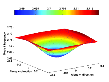
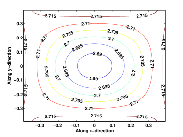
Figure 6: Variation of fundamental frequency as a function of crack position for a simply supported square FGM plate. The crack orientation, $\theta$ is taken to be 0, i.e., horizontal crack.

Plate with multiple cracks

Figure (7) shows a plate with two cracks with lengths $a_{1}$ and $a_{2}$ and with orientations $\theta_{1}$ and $\theta_{2}$ they subtend with the horizontal. The effect of respective crack orientation on the fundamental frequency for a simply supported FGM plate is numerically studied. The horizontal and vertical separation (see Figure (7)) between the crack tips is set to a constant value, $H=$0.2 and $V=$0.1, respectively. Table 8 shows the variation of fundamental frequency for plate with gradient index $n=$5 and crack lengths $a_{1}=a_{2}=$ 0.2 as a function of crack orientations. Figure (8) shows the variation of frequency as a function of orientation of one crack for different orientations of the second crack. It can be seen that with increase in crack orientation, the frequency initially decreases until it reaches a mimimum at $\theta=45^{o}$. With further increase in crack orientation, the frequency increases and reaches maximum at $\theta_{1}=\theta_{2}=$90^o. The frequency value at $\theta=0^{o}$ is not the same as that at $\theta=90^{o}$ as we would expect. This is because when $\theta_{1}=\theta_{2}=90^{o}$, the crack is located away from the center of the plate and crack disturbs the mode shape slightly.

Figure 7: Plate with multiple cracks: geometry

Table 8: Fundamental frequency $\omega b^{2}/h\sqrt{\rho_{c}/E_{c}}$ for simply supported Si₃N₄/SUS304 FGM square plate, gradient index, $n=$5. ^†denotes change in trend.

Crack	Crack orientation, $\theta_{2}$.
Orientation, $\theta_{1}$	0	10	20	30	40	45	50†	60	70	80	90
0	2.6149	2.6122	2.6077	2.6034	2.5997	2.5988	2.5981	2.5993	2.6023	2.6066	2.6098
10	2.6122	2.6094	2.6049	2.6006	2.5969	2.5960	2.5953	2.5964	2.5994	2.6037	2.6068
20	2.6077	2.6049	2.6004	2.5961	2.5924	2.5914	2.5907	2.5919	2.5948	2.5991	2.6022
30	2.6034	2.6006	2.5961	2.5918	2.5881	2.5871	2.5864	2.5876	2.5905	2.5948	2.5979
40	2.5997	2.5969	2.5924	2.5881	2.5844	2.5835	2.5827	2.5839	2.5868	2.5910	2.5941
45	2.5987	2.5959	2.5914	2.5871	2.5834	2.5825	2.5818	2.5829	2.5858	2.5901	2.5931
50†	2.5980	2.5952	2.5907	2.5864	2.5827	2.5818	2.5811	2.5822	2.5851	2.5893	2.5924
60	2.5992	2.5964	2.5918	2.5876	2.5839	2.5829	2.5822	2.5834	2.5863	2.5905	2.5935
70	2.6022	2.5993	2.5948	2.5905	2.5868	2.5858	2.5851	2.5863	2.5891	2.5933	2.5963
80	2.6065	2.6036	2.5990	2.5947	2.5910	2.5900	2.5893	2.5904	2.5933	2.5974	2.6004
90	2.6098	2.6069	2.6022	2.5979	2.5942	2.5932	2.5924	2.5935	2.5964	2.6005	2.6035

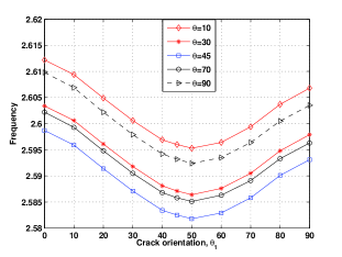
(a) Effect of crack orientation, $\theta$

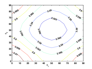
(b) Effect of gradient index, $n$

Figure 8: Variation of fundamental frequency for a simply supported square Si₃N₄/SUS304 FGM plate with a center crack as a function crack orientation with $H=$0.2, $V=$0.1 and $a/h=$10 (see Figure (7)).

Effect of aspect ratio, thickness and boundary conditions

The influence of plate aspect ratio $b/a$, plate thickness $a/h$ and boundary condition on a cracked FGM plate with a horizontal center crack is shown in Table 9. Two types of boundary conditions are studied: Simply supported (SS) and Clamped condition (CC). For a given crack length and for a given crack location, decreasing the plate thickness and increasing the plate aspect ratio, increases the frequency. The increase in stiffness is the cause for increase in frequency when the boundary condition is changed from SS to CC for a fixed aspect ratio and plate thickness.

Table 9: Effect of plate aspect ratio $b/a$, plate thickness $a/h$ and boundary condition on fundamental frequency $\omega b^{2}/h\sqrt{\rho_{c}/E_{c}}$ for Si₃N₄/SUS304 FGM plate with horizontal center crack $(c_{y}/b=0.5,d/a=0.5)$. ^†Simply Supported, ^∗Clamped Support.

$b/a$	$a/h$	Mode 1			Mode 2
		SS†	CC∗		SS†	CC∗
0.5	10	1.1205	2.2202		2.1586	2.8588
	20	1.1974	2.5043		2.5482	3.4621
	100	1.2625	2.6748		2.6593	4.0903
1	10	2.4051	4.1624		5.2792	6.6286
	20	2.4831	4.4592		5.8338	7.6464
	100	2.5473	4.6311		6.2765	8.5774
2	10	6.6864	12.7513		10.5295	15.9115
	20	6.8101	13.4551		10.8647	17.0301
	100	6.8847	13.7540		11.0392	17.6030

4.2 Plate with side crack

Consider a plate of uniform thickness, $h$, with length and width as $a$ and $b$, respectively. Figure (9) shows a cantilevered plate with a side crack of length $d$ located at a distance of $c_{y}$ from the x-axis and at an angle $\theta$ with respect to the $x-$ axis. The influence of plate thickness, crack orientation and gradient index on the fundamental frequency is shown in Table 10 and in Figure (10). With increase in gradient index $n$, the frequency decreases for all crack orientations and for different plate thickness. With increase in crack orientation from $\theta=-60^{o}$ to $\theta=60^{o}$, the frequency initially decreases until $\theta=-40^{o}$ and then reaches the maximum when the crack is horizontal. And with further increase in the crack orientation, the frequency decreases and the plate’s response is symmetric. This is because, when the crack is horizontal $(\theta=0)$, the crack is aligned to the first mode shape and the response of the plate is similar to the cantilevered plate without a crack. The frequency of the plate without a crack is greater than a plate with a crack. Figures (11) and (12) shows first two mode shapes for a cantilevered plate with and without a horizontal crack. As explained earlier the frequency and the first mode shape for a plate with and without a crack are very similar. For any other crack orientation, the mode shape would be influenced by the presence of the crack. Figures (13) and (14) shows the first mode shape of a cantilevered plate with a side crack with orientations $\theta=\pm 40^{o}$ and $\theta=\pm 60^{o}$, respectively.

Figure 9: Cantilevered plate with a side crack: geometry

Table 10: Fundamental frequency $\omega b^{2}/h\sqrt{\rho_{c}/E_{c}}$ for cantilevered square plate Si₃N₄/SUS304 FGM plate with a side crack $(c_{y}/b=0.5,d/a=0.5)$ as a function of crack angle and gradient index. ^†denotes change in trend.

$a/h$	crack	gradient index, $n$
	angle, $\theta$	0	1	2	5	10
10	-60	0.9859	0.5918	0.5322	0.4838	0.4610
	-50	0.9840	0.5906	0.5312	0.4829	0.4601
	-40†	0.9838	0.5905	0.5311	0.4828	0.4600
	-30	0.9862	0.5919	0.5323	0.4840	0.4611
	-20	0.9900	0.5943	0.5344	0.4859	0.4630
	-10	0.9936	0.5964	0.5364	0.4876	0.4646
	0†	0.9951	0.5973	0.5372	0.4884	0.4653
	10	0.9936	0.5964	0.5364	0.4876	0.4646
	20	0.9900	0.5943	0.5344	0.4859	0.4630
	30	0.9862	0.5919	0.5323	0.4840	0.4611
	40†	0.9838	0.5905	0.5311	0.4828	0.4600
	50	0.9840	0.5906	0.5312	0.4829	0.4601
	60	0.9859	0.5918	0.5322	0.4838	0.4610
20	-60	0.9949	0.5972	0.5371	0.4883	0.4653
	-50	0.9927	0.5959	0.5359	0.4872	0.4643
	-40†	0.9924	0.5957	0.5357	0.4871	0.4641
	-30	0.9944	0.5969	0.5368	0.4881	0.4651
	-20	0.9979	0.5989	0.5387	0.4898	0.4667
	-10	1.0011	0.6009	0.5404	0.4913	0.4682
	0†	1.0024	0.6016	0.5411	0.4920	0.4688
	10	1.0011	0.6009	0.5404	0.4913	0.4682
	20	0.9979	0.5989	0.5387	0.4898	0.4667
	30	0.9944	0.5969	0.5368	0.4881	0.4651
	40†	0.9924	0.5957	0.5357	0.4871	0.4641
	50	0.9927	0.5959	0.5359	0.4872	0.4643
	60	0.9949	0.5972	0.5371	0.4883	0.4653

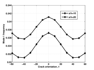
(a) Effect of aspect ratio, $a/h$

(b) Effect of gradient index, $n$

Figure 10: Variation of fundamental frequency for a cantilevered square Si₃N₄/SUS304 FGM plate with a side crack as a function of crack orientation. $d/a=$0.5, $c_{y}/a$=0.5.

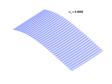
(a) Without crack, $\omega_{1}=$0.4885

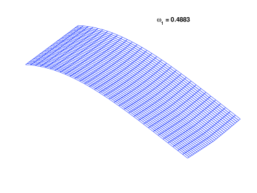
(b) With crack, $\omega_{1}=$0.4883

Figure 11: First Mode shape for a cantilevered plate with a side crack with $\theta=0,n=5,c_{y}/b=0.5,d/a=0.5,a/h=10,b/a=1$.

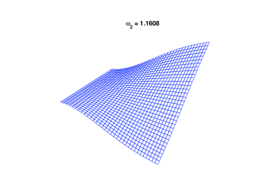
(a) Without crack, $\omega_{2}=$1.1608

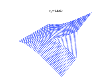
(b) With crack, $\omega_{2}=$0.8223

Figure 12: Second Mode shape for a cantilevered plate with a side crack with $\theta=0,n=5,c_{y}/b=0.5,d/a=0.5,a/h=10,b/a=1$.

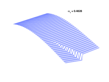
(a) $\theta=40^{o}$

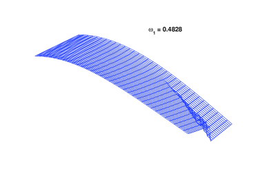
(b) $\theta=-40^{o}$

Figure 13: First Mode shape $(\omega_{1}=0.4828)$ for a cantilevered plate with a side crack with $n=5,c_{y}/b=0.5,d/a=0.5,a/h=10,b/a=1$.

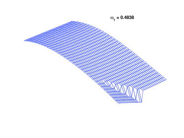
(a) $\theta=60^{o}$

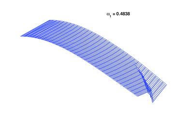
(b) $\theta=-60^{o}$

Figure 14: First Mode shape $(\omega_{1}=0.4838)$ for a cantilevered plate with a side crack with $n=5,c_{y}/b=0.5,d/a=0.5,a/h=10,b/a=1$.

5 Conclusion

Natural frequencies of cracked functionally graded material plate is studied using the extended finite element method. The formulation is based on first order shear deformation theory for plates and a four-noded field consistent enriched element is used. The material is assumed to be temperature dependent and graded in the thickness direction. Numerical experiments have been conducted to bring out the effect of gradient index, crack length, crack orientation, crack location, boundary condition, plate aspect ratio and plate thickness on the natural frequency of the FGM plate. Also the influence of multiple cracks and their relative orientation on the natural frequency is studied. From the detailed numerical study, the following can be concluded:

• Increasing the crack length decreases the natural frequency. This is due to the reduction in stiffness of the material structure. The frequency is lowest when the crack is located at the center of the plate.

• Increasing gradient index $n$ decreases the natural frequency. This is due to the increase in metallic volume fraction.

• Decreasing the plate thickness $a/h$ and increasing the aspect ratio $b/a$ increases the frequency.

• For a cantilevered plate with a side crack, horizontal crack has the maximum frequency and the trend changes at $\theta=\pm 40^{o}$.

• Crack orientation $\theta=45^{o}$ has been observed to be a critical angle. At this crack orientation, the frequency changes its trend for a square plate.

• Increasing the number of cracks, decreases the overall stiffness of the plate and thus decreasing the frequency. The frequency is lowest when both the cracks are oriented at $\theta=50^{o}$.

Acknowledgements

S Natarajan acknowledges the financial support of (1) the Overseas Research Students Awards Scheme; (2) the Faculty of Engineering, University of Glasgow, for period Jan. 2008 - Sept. 2009 and of (3) the School of Engineering (Cardiff University) for the period Sept. 2009 onwards.

S Bordas would like to thank the support of the Royal Academy of Engineering and of the Leverhulme Trust for his Senior Research Fellowship entitled “Towards the next generation surgical simulators” as well as the support of EPSRC under grants EP/G042705/1 Increased Reliability for Industrially Relevant Automatic Crack Growth Simulation with the eXtended Finite Element Method.

References

- [1] M. Koizumi, The concept of FGM, Ceram. Trans. Funct. Graded Mater 34 (1993) 3–10.
- [2] M. Koizumi, FGM activities in Japan, Composites 28 (1997) 1–4.
- [3] S. Vel, R. Batra, Three-dimensional exact solution for the vibration of functionally graded rectangular plates, Journal of Sound and Vibration 272 (2004) 703–730.
- [4] H. Matsunaga, Free vibration and stability of functionally graded plates according to a 2-D higher-order deformation theory, Composite Structures 82 (2008) 499–512.
- [5] X. He, T. Ng, S. Sivashankar, K. Liew, Active control of fgm plates with integrated piezoelectric sensors and actuators, International Journal of Solids and Structures 38 (2001) 1641–1655.
- [6] K. Liew, X. He, T. Ng, S. Sivashankar, Active control of fgm plates subjected to a temperature gradient: modeling via finite element method based on FSDT, International Journal for Numerical Methods in Engineering 52 (2001) 1253–1271.
- [7] T. Ng, K. Lam, K. Liew, Effect of FGM materials on parametric response of plate structures, Computer Methods in Applied Mechanics and Engineering 190 (2000) 953–962.
- [8] J. Yang, H. Shen, Vibration characteristic and transient response of shear-deformable functionally graded plates in thermal environments, Journal of Sound and Vibration 255 (2002) 579–602.
- [9] A. Ferreira, R. Batra, C. Roque, L. Qian, R. Jorge, Natural frequencies of functionally graded plates by a meshless method, Composite Structures 75 (2006) 593–600.
- [10] J. Yang, H. Shen, Dynamic response of initially stressed functionally graded rectangular thin plates, Composite Structures 54 (2001) 497–508.
- [11] L. Qian, R. Batra, L. Chen, Static and dynamic deformations of thick functionally graded elastic plates by using higher order shear and normal deformable plate theory and meshless local petrov galerkin method, Composites Part B: Engineering 35 (2004) 685–697.
- [12] J. Reddy, Analysis of functionally graded plates, International Journal for Numerical Methods in Engineering 47 (2000) 663–684.
- [13] A. A. R, A. Bagri, S. Bordas, T. Rabczuk, Analysis of thermoelastic waves in a two-dimensional functionally graded materials domain by the meshless local Petrov-Galerkin method, Computer Modelling in Engineering and Science 65 (2010) 27–74.
- [14] P. Lynn, N. Kumbasar, Free vibrations of thin rectangular plates having narrow cracks with simply supported edges, Dev. Mech 4 (1967) 928–991.
- [15] B. Stahl, L. Keer, Vibration and stability of cracked rectangular plates., International Journal of Solids and Structures 8 (1972) 69–91.
- [16] R. Solecki, Bending vibration of rectangular plate with arbitrarly located rectilinear crack, Engineering Fracture Mechanics 22 (4) (1985) 687–695.
- [17] S. Khadem, M. Rezaee, Introduction of modified comparison functions for vibration analysis of a rectangular cracked plate., Journal of Sound and Vibration 236 (2) (2000) 245–258.
- [18] G. Wu, Y. Shih, Dynamic instability of rectangular plate with an edge cracked, Computers and Structures 84 (1-2) (2005) 1–10.
- [19] G. Qian, S. Gu, J. Jiang, A finite element model of cracked plates and application to vibration problems, Computers and Structures 39 (5) (1991) 483–487.
- [20] H. Lee, S. Lim, Vibration of cracked rectangular plates including transverse shear deformation and rotary inertia, Computers and Structures 49 (4) (1993) 715–718.
- [21] C. Huang, O. M. III, M. Chang, Vibrations of cracked rectangular FGM thick plates, Commposite Structuresdoi:10.1016/j.compstruct.2011.01.005.
- [22] S. Kitipornchai, L. Ke, J. Y. andY Xiang, Nonlinear vibration of edge cracked functionally graded Timoshenko beams, Journal of Sound and Vibration 324 (2009) 962–982.
- [23] J. Yang, Y. Hao, W. Zhang, S. Kitipornchai, Nonlinear dynamic response of a functionally graded plate with a through-width surface crack, Nonlinear Dynamics 59 (2010) 207–219.
- [24] B. Somashekar, G. Prathap, C. R. Babu, A field-consistent four-noded laminated anisotropic plate/shell element, Computers and Structures 25 (1987) 345–353.
- [25] M. Bachene, R. Tiberkak, S. Rechak, Vibration analysis of cracked plates using the extended finite element method, Arch. Appl. Mech. 79 (2009) 249–262. doi:10.1007/s00419-008-0224-7.
- [26] M. Bachene, R. Tiberkak, S. Rechak, G. Maurice, B. Hachi, Enriched finite element for modal analysis of cracked plates, in: Damage and Fracture Mechanics: Failure Analysis and Engineering Materials and Structures, Springer Science, 2009, pp. 463–471.
- [27] R. Tiberkak, M. Bachene, B. Hachi, S. Rechak, M. Haboussi, Dynamic response of cracked plate subjected to impact loading using the extended finite element method, in: Damage and Fracture Mechanics: Failure Analysis and Engineering Materials and Structures, Springer Science, 2009, pp. 297–306.
- [28] T. Mori, K. Tanaka, Average stress in matrix and average elasticenergy of materials with misfitting inclusions, Acta Metallurgica 21 (1973) 571–574.
- [29] Y. Benvensite, A new approach to the application of mori–tanaka’s theory in composite materials, Mechanics of Materials 6 (1987) 147–157.
- [30] Z.-Q. Cheng, R. Batra, Three dimensional thermoelastic deformations of a functionally graded elliptic plate, Composites Part B: Engineering 2 (2000) 97–106.
- [31] J. Reddy, C. Chin, Thermomechanical analysis of functionally graded cylinders and plates, Journal of Thermal Stresses 21 (1998) 593–629.
- [32] S. Rajasekaran, D. Murray, Incremental finite element matrices, ASCE Journal of Structural Divison 99 (1973) 2423–2438.
- [33] M. Ganapathi, T. Varadan, B. Sarma, Nonlinear flexural vibrations of laminated orthotropic plates, Computers and Structures 39 (1991) 685–688.
- [34] I. Babuška, G. Caloz, J. Osborn, Special finite element methods for a class of second order elliptic problems with rough coefficients, SIAM Journal of Numerical Analysis 31 (1994) 945–981.
- [35] T. Belytschko, T. Black, Elastic crack growth in finite elements with minimal remeshing, International Journal for Numerical Methods in Engineering 45 (1999) 601–620.
- [36] J. M. Melenk, On generalized finite element methods, Ph.D. thesis, University of Maryland, College Park, MD (1995).
- [37] C. A. Duarte, T. J. Liszka, W. W. Tworzydlo, Clustered generalized finite element methods for mesh unrefinement, non-matching and invalid meshes, International Journal for Numerical Methods in Engineering 69 (11) (2007) 2409–2440. doi:10.1002/nme.1862.
- [38] I. Babuška, J. Melenk, The partition of unity finite element method, International Journal for Numerical Methods in Engineering 40 (1997) 727–758.
- [39] I. Babuska, V. Nistor, N. Tarfulea, Generalized finite element method for second-order elliptic operators with dirichlet boundary conditions, Journal of Computational and Applied Mathematics 218 (1) (2008) 175–183. doi:10.1016/j.cam.2007.04.041.
- [40] A. Simone, C. Duarte, E. V. der Giessen, A generalized finite element method for polycrystals with discontinuous grain boundaries, International Journal for Numerical Methods in Engineering 67 (2006) 1122–1145.
- [41] B. Karihaloo, Q. Xiao, Modelling of stationary and growing cracks in FE framework without remeshing: a state-of-the-art review, Computers and Structures 81 (3) (2003) 119–129. doi:10.1016/S0045-7949(02)00431-5.
- [42] A. Yazid, N. Abdelkader, H. Abdelmadjid, A state-of-the-art review of the x-fem for computational fracture mechanics, Applied Mathematical Modelling 33 (12) (2009) 4269–4282. doi:10.1016/j.apm.2009.02.010.
- [43] S. Bordas, P. V. Nguyen, C. Dunant, A. Guidoum, H. Nguyen-Dang, An extended finite element library, International Journal for Numerical Methods in Engineering 71 (2007) 703–732.
- [44] T. Rabczuk, S. Bordas, G. Zi, On three-dimensional modelling of crack growth using partition of unity methods, Computers and Structures 88 (2010) 1391–1411.
- [45] J. Dolbow, N. Moës, T. Belytschko, Modeling fracture in mindlin-reissner plates with the extended finite element method, International Journal of Solids and Structures 37 (48-50) (2000) 7161–7183. doi:10.1016/S0020-7683(00)00194-3.
- [46] N. Moës, J. Dolbow, T. Belytschko, A finite element method for crack growth without remeshing, International Journal for Numerical Methods in Engineering 46 (1) (1999) 131–150.
- [47] D. S. Watkins, Fundamentals of matrix computations, Wiley Publishers, 2002.
- [48] N. Sundararajan, T. Prakash, M. Ganapathi, Nonlinear free flexural vibrations of functionally graded rectangular and skew plates under thermal environments, Finite Elements in Analysis and Design 42 (2) (2005) 152–168.
- [49] T. Prakash, N. Sundararajan, M. Ganapathi, On the nonlinear axisymmetric dynamic buckling behavior of clamped functionally graded spherical caps, Journal of Sound and Vibration 299 (2007) 36–43.
- [50] M. Singh, T. Prakash, M. Ganapathi, Finite element analysis of functionally graded plates under transverse load, Finite Elements in Analysis and Design 47 (2011) 453–460.
- [51] C. Huang, A. Lieissa, Vibration analysis of rectangular plates with side cracks via the Ritz method, Journal of Sound and Vibration 323 (2009) 974–988.