Fermion spectrum and localization on kinks in a deconstructed dimension

Abstract

We study the deconstructed scalar theory having nonlinear interactions and being renormalizable. It is shown that the kink-like configurations exist in such models. The possible forms of Yukawa coupling are considered. We find the degeneracy in mass spectrum of fermions coupled to the nontrivial scalar configuration.

I Introduction

The concept of the brane and brane world exhibits broad possibilities in the particle theory beyond the standard model. In the early stage of study on the higher dimensional theories, it has been considered that we may live in a domain wall perpendicular to the fifth dimension dw . The domain wall may be described by a kink configuration of an self-interacting scalar field. The matter field which couples to the kink is localized in the extra dimension and acquires a mass spectrum consisting both discrete and continuum modes in general.

Even if we consider the model with a compact dimension, the kink or solitonic configuration is expected to play important roles. The localization of fermions due to solitonic domain walls can explain the hierarchy in masses and the Yukawa couplings ex . The compactified dimension is taken as $S^{1}$ or $S^{1}/Z_{2}$ in such a case. The kink solutions in the periodic compact space are known to be topologically unstable like sphalerons. They have been studied by some authors sph .

In the recent decade, another approach to the particle physics models has been explored. The idea of dimensional deconstruction DD is to construct the models mimicking the higher dimensional gauge theory from the four dimensional gauge theory. In some sense, the deconstruction means introducing the discrete extra space into the theory. Some merits of higher dimensional theory can be inherited by four dimensional theory, whose high-energy behavior can be well controlled.

Therefore it is worth examining the ‘deconstructed kink model’ in the framework of four dimensional theory. Fortunately, discrete models for kink-like solutions have been considered apart from particle physics Speight . Thus we must study the solutions with specific boundary conditions and especially coupling to fermions to apply the discrete models to particle physics.

Most general starting point is to consider the multi-scalar model in four dimensions, whose Lagrangian density reads

$${\cal L}=\frac{1}{2}\sum_{i=1}^{N}\partial^{\mu}\phi_{i}\partial_{\nu}\phi_{i}-V(\phi_{1},\phi_{2},\ldots,\phi_{N})\,,$$ (1)

where $\phi_{i}$ are real scalar fields and $V$ is the potential. Unlike the original dimensional deconstruction scheme, the gauge invariance is not assumed. Moreover even if the continuum limit is uniquely defined, it is known that the discretized action can be exhibited by various different forms Speight . Since the other guiding principles are needed for detailed study, we will refer the supersymmetric model as shown later.

The original dimensional deconstruction is found to be associated with the graph structure KS . Thus we begin with considering the bilinear term in scalar fields and construct the interaction terms on vertices or edges of a graph taking the correspondence with the continuum theory into consideration.

In the next section, we review the kink solution in $(1+1)$-dimensional field theory. Since we must include fermions later, we consider a supersymmetric theory; the structure of this theory will be referred in the later sections. In Sec. III, we consider discretized or deconstructed free scalar models, whose continuum limit is the compactified theory with $S^{1}$ or $S^{1}/Z_{2}$. In Sec. IV, we choose the form of the scalar interactions, which is expected to make the ‘discrete kink’ configurations possible. The result of numerical calculations on the solitonic solutions is shown in Sec. V. In Sec. VI, we consider the Yukawa coupling of fermions and scalars. Various ‘discrete’ versions of the Yukawa coupling are possible, though their ‘continuum’ limits are all the same one. In this paper, we consider the models whose couplings are similar to those of the supersymmetric model mentioned in Sec. II in the continuum limit. The numerical result for the fermionic spectra is exhibited in Sec. VII. The last section is devoted to summary and prospects.

II kink solutions in the continuum theory

In this section, we review a continuum theory for kink solutions Raj . The form of the action is used to determine the way for discretization of bosonic as well as fermionic sector later.

We consider the $(1+1)$-dimensional supersymmetric field theory, whose Lagrangian density is

$${\cal L}=\frac{1}{2}(\partial\phi)^{2}-\frac{1}{2}\left(\frac{\partial W(\phi)}{\partial\phi}\right)^{2}+\frac{1}{2}i\bar{\psi}\partial\!\!\!/\psi-\frac{1}{2}\frac{\partial^{2}W(\phi)}{\partial\phi^{2}}\bar{\psi}\psi\,,$$ (2)

where we choose the superpotential $W(\phi)$ as

$$W(\phi)=g\left(\frac{\phi^{3}}{3}-a^{2}\phi\right)\,,$$ (3)

with $g$ and $a$ are constants.

Then the bosonic part of the Lagrangian density reads

$${\cal L}_{B}=\frac{1}{2}(\partial\phi)^{2}-\frac{1}{2}g^{2}\left(\phi^{2}-a^{2}\right)^{2}\,,$$ (4)

and thus we find the equation of motion as

$$-\partial_{t}^{2}\phi+\partial_{x}^{2}\phi-2g^{2}(\phi^{2}-a^{2})\phi=0\,.$$ (5)

A non trivial static solution, a kink solution, satisfies the equation of motion, and expressed as

$$\phi_{0}(x)=a\tanh gax\,,$$ (6)

where we set an integration constant for $\phi_{0}(0)=0$. One can find that this solution also satisfies

$$\partial_{x}\phi+g\left(\phi^{2}-a^{2}\right)=\partial_{x}\phi+\frac{\partial W}{\partial\phi}=0\,.$$ (7)

The coupling of the scalar and the (Majorana) fermion is proportional to $-g\phi\bar{\psi}\psi$. In the present case, it is not surprising and is of the usual Yukawa form. This coupling with general coupling constant (say, $-G\phi\bar{\psi}\psi$) or similar type of models have been investigated in the soliton physics DJR .

The solitonic configurations in the periodic compact space have also been considered in several authors sph . It has been shown that he nature of quasi-stable solutions depends on the size of the compact space. A solution of (7) is not necessarily a solution of the equation of motion in the compact space. Interestingly, these features are also true in some sense for the case of discrete solitons studied in Sec. IV.

III deconstructing a free scalar field theory and a graph

Suppose $N$ real scalar fields $\phi_{i}$ $(i=1,\dots,N)$. The mass spectrum of the scalars is the same as that of the vector bosons in the dimensional deconstruction model DD , if the action is given by

$${\cal L} = \sum_{i=1}^{N}\frac{1}{2}(\partial\phi_{i})^{2}-\frac{1}{2}f^{2}\sum_{i}({{\it\Delta}}\phi_{i})^{2}$$ (8)

$$= \sum_{i=1}^{N}\frac{1}{2}(\partial\phi_{i})^{2}-\frac{1}{2}f^{2}\sum_{i}(\phi_{i+1}-\phi_{i})^{2}\,,$$

where ${\it\Delta}\phi_{i}\equiv\phi_{i+1}-\phi_{i}$ and $f$ is a mass scale. In the four-dimensional point of view, we can say that the potential is of a ‘difference-squared’ type.

The sum in the potential is interpreted as $\phi_{N+1}\equiv\phi_{1}$ and from $i=1$ to $N$. Then the large $N$ limit leaving $L\equiv N/f$ constant leads to the five dimensional scalar theory with $S^{1}$ (Kaluza-Klein) compactification. Namely, the $N\times N$ mass-square matrix in this model is

$$f^{2}\left(\begin{array}[]{cccccc}2&-1&0&\cdots&0&-1\\ -1&2&-1&\cdots&0&0\\ 0&-1&2&\cdots&0&0\\ \vdots&\vdots&\vdots&\vdots&\vdots&\vdots\\ 0&0&0&\cdots&2&-1\\ -1&0&0&\cdots&-1&2\end{array}\right)\equiv f^{2}{\Delta}(C)\,,$$ (9)

and the eigenvalues are

$$4f^{2}\sin^{2}\frac{k\pi}{N}\qquad(k=0,1,\ldots,N-1)\,,$$ (10)

which becomes $(2\pi k/L)^{2}$ in the large $N$ limit mentioned above. Here $L$ corresponds to the circumference of $S^{1}$.

The other summation rule is possible. The sum in the expression (8) is taken from $i=1$ to $N-1$. In this case the $N\times N$ mass-square matrix becomes

$$f^{2}\left(\begin{array}[]{cccccc}1&-1&0&\cdots&0&0\\ -1&2&-1&\cdots&0&0\\ 0&-1&2&\cdots&0&0\\ \vdots&\vdots&\vdots&\vdots&\vdots&\vdots\\ 0&0&0&\cdots&2&-1\\ 0&0&0&\cdots&-1&1\end{array}\right)\equiv f^{2}{\Delta}(P)\,,$$ (11)

and its eigenvalues are

$$4f^{2}\sin^{2}\frac{k\pi}{2N}\qquad(k=0,1,\ldots,N-1)\,,$$ (12)

and the large $N$ limit yields the theory with the compactification on $S^{1}/Z_{2}$.

In conclusion so far, the construction of the potential is associated with the structure of a graph, in the sense of graph theory graphtheory . A graph consists of vertices and edges each of which connects two vertices. The edge $e$ connects the vertices $o(e)$ and $t(e)$. The vertex $o(e)$ means the origin of the edge $e$ while the vertex $t(e)$ means the terminus of the edge $e$. We assign $N$ scalar fields onto $N$ vertices of the graph and their action is written by

$${\cal L}=\sum_{v\in{\cal V}}\frac{1}{2}(\partial\phi_{v})^{2}-\frac{1}{2}f^{2}\sum_{e\in{\cal E}}(\phi_{t(e)}-\phi_{o(e)})^{2}\,,$$ (13)

where ${\cal V}$ and ${\cal E}$ denote the set of vertices and edges, respectively.

Now we can express the mass term by using the incidence matrix $E$ defined as

$$(E)_{ve}=\left\{\begin{array}[]{cc}1&{\rm if~{}}v=o(e)\\ -1&{\rm if~{}}v=t(e)\\ 0&{\rm otherwise}\end{array}\right.\,,$$ (14)

since in both cases, the difference ${\it\Delta}\phi$ is defined as associated with each edge such that

$$({\it\Delta}\phi)_{e}=\phi_{t(e)}-\phi_{o(e)}=-\sum_{v\in{\cal V}}(E^{T})_{ev}\phi_{v}\,,$$ (15)

and then

$$\sum_{e\in{\cal E}}(\phi_{t(e)}-\phi_{o(e)})^{2}=\sum_{v,v^{\prime}\in{\cal V}}\sum_{e\in{\cal E}}\phi_{v^{\prime}}(E)_{v^{\prime}e}(E^{T})_{ev}\phi_{v}\,,$$ (16)

where the matrix $E^{T}$ is the transposed matrix of $E$.

For the first case introduced in this section, the incidence matrix is

$$E(C)=\left(\begin{array}[]{ccccc}1&0&\cdots&0&-1\\ -1&1&\cdots&0&0\\ 0&-1&\cdots&0&0\\ \vdots&\vdots&\ddots&\vdots&\vdots\\ 0&0&\cdots&1&0\\ 0&0&\cdots&-1&1\end{array}\right)\,,$$ (17)

and its transposed matrix is

$$E^{T}(C)=\left(\begin{array}[]{cccccc}1&-1&0&\cdots&0&0\\ 0&1&-1&\cdots&0&0\\ \vdots&\vdots&\vdots&\ddots&\vdots&\vdots\\ 0&0&0&\cdots&1&-1\\ -1&0&0&\cdots&0&1\end{array}\right)\,.$$ (18)

The corresponding graph is the cycle graph in the term of graph theory (Fig. 1).

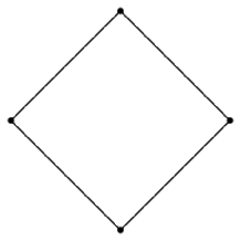
Figure 1: The cycle graph $C_{4}$ and the path graph $P_{4}$. Each suffix indicates the number of vertices in the graph.

Note that $\Delta(C)=E(C)E^{T}(C)$, where $\Delta(C)$ is known as a graph Laplacian for a cycle graph.

For the second case introduced in this section, the incidence matrix is

$$E(P)=\left(\begin{array}[]{cccc}1&0&\cdots&0\\ -1&1&\cdots&0\\ 0&-1&\cdots&0\\ \vdots&\vdots&\ddots&\vdots\\ 0&0&\cdots&1\\ 0&0&\cdots&-1\end{array}\right)\,,$$ (19)

and its transposed matrix is

$$E^{T}(P)=\left(\begin{array}[]{cccccc}1&-1&0&\cdots&0&0\\ 0&1&-1&\cdots&0&0\\ \vdots&\vdots&\vdots&\ddots&\vdots&\vdots\\ 0&0&0&\cdots&1&-1\end{array}\right)\,.$$ (20)

The corresponding graph is the path graph in the term of graph theory (Fig. 1). Note that $\Delta(P)=E(P)E^{T}(P)$, where $\Delta(P)$ is known as a graph Laplacian for a path graph.

In the next section, we will examine the nonlinear interaction of scalars, which is essential for the kink-like configurations, by referring the graph structure.

IV deconstructing the scalar potential

In the previous section, the term corresponding to the kinetic term of the scalar theory has been simply discretized. However, we should consider some constraints to the interaction term in the discretized action, because there are many possible descretizations which have the same continuum limit.

First of all, we want to avoid apparently complicated interactions. We postulate renormalizability, at least superficially. At most four scalar fields coupled mutually at a point in four dimensions. Secondly, we wish to consider models possessing a continuum limit for a large number of four-dimensional scalar field. In this limit, the static configuration is much alike kinks or sphalerons on $S^{1}/Z_{2}$ or $S^{1}$. Thirdly, the structure of the interaction should reflect a graph structure. The deconstructed ‘kinetic term’ is expressed as a sum over edges of a graph as shown in the previous section, so the deconstructed interaction term should also be written as a sum of the contribution assigned at edges.

Now the possible Lagrangian density is the following:

$${\cal L}=\sum_{v\in{\cal V}}\frac{1}{2}(\partial\phi_{v})^{2}-\frac{1}{2}f^{2}\sum_{e\in{\cal E}}(\phi_{t(e)}-\phi_{o(e)})^{2}-\frac{1}{2}\sum_{e\in{\cal E}}g^{2}\left(\frac{p\phi_{t(e)}^{2}+q\phi_{t(e)}\phi_{o(e)}+p\phi_{o(e)}^{2}}{2p+q}-a^{2}\right)^{2}\,,$$ (21)

where $p$ and $q$ are dimensionless constants and we consider only a path graph or a cycle graph, corresponding to the continuum theory on $S^{1}/Z_{2}$ or $S^{1}$, respectively.

For a cycle or path graph, the potential term in the sense of the four-dimensional theory is

$$V=\frac{1}{2}f^{2}\sum_{i}(\phi_{i+1}-\phi_{i})^{2}+\frac{1}{2}\sum_{i}g^{2}\left(\frac{p\phi_{i+1}^{2}+q\phi_{i+1}\phi_{i}+p\phi_{i}^{2}}{2p+q}-a^{2}\right)^{2}\,.$$ (22)

Setting the derivative with respect to $\phi_{k}$ ($k$ is not $1$ or $N$ for the case with a path graph) to zero yields the recurrence relation among three terms. Unfortunately, it seems that this recurrence relation cannot be satisfied by multiple use of some recurrence relations in two terms. Thus for a finite number of fields, similar relations to the continuum theory like (7) cannot hold.

Because this is still far from a specific model due to arbitrary numbers $p$ and $q$, we select the case by special conditions $p=q=1$. This selection was adopted first by Speight and Ward (in Speight ). In this case, we find

$$g\left(\frac{\phi_{i+1}^{2}+\phi_{i+1}\phi_{i}+\phi_{i}^{2}}{3}-a^{2}\right){\it\Delta}\phi_{i} = g\left(\frac{\phi_{i+1}^{2}+\phi_{i+1}\phi_{i}+\phi_{i}^{2}}{3}-a^{2}\right)(\phi_{i+1}-\phi_{i})$$

$$=g\left(\frac{\phi_{i+1}^{3}-\phi_{i}^{3}}{3}-a^{2}(\phi_{i+1}-\phi_{i})\right) = W(\phi_{i+1})-W(\phi_{i})\,.$$ (23)

This relation shows that the derivative of the superpotential $\frac{\partial W}{\partial\phi}$ is replaced by the difference $\frac{{\it\Delta}W}{{\it\Delta}\phi}$, or

$${\it\Delta}W=-E^{T}W\,,\quad{\rm where}~{}~{}W=\left(\begin{array}[]{c}W(\phi_{1})\\ W(\phi_{2})\\ \vdots\\ W(\phi_{N})\end{array}\right).$$

Thus in this case, we can say that the interaction terms is related to the graph structure.

For $p=q=1$, which we concentrate on this case hereafter, the potential minimum is given by the simultaneous equations

$$\frac{\partial V}{\partial\phi_{k}} = -f^{2}(\phi_{k+1}-2\phi_{k}+\phi_{k-1})+g^{2}\left(\frac{\phi_{k+1}^{2}+\phi_{k+1}\phi_{k}+\phi_{k}^{2}}{3}-a^{2}\right)\frac{\phi_{k+1}+2\phi_{k}}{3}$$ (24)

$$+g^{2}\left(\frac{\phi_{k}^{2}+\phi_{k}\phi_{k-1}+\phi_{k-1}^{2}}{3}-a^{2}\right)\frac{2\phi_{k}+\phi_{k-1}}{3}=0\,,$$

where $k$ is not $1$ or $N$ for the case with a path graph. To obtain static scalar configurations, we should solve the recursion relation (24) for a cycle graph, and for a path graph with additional ‘boundary’ equations,

$$\frac{\partial V}{\partial\phi_{1}} = -f^{2}(\phi_{2}-\phi_{1})+g^{2}\left(\frac{\phi_{2}^{2}+\phi_{2}\phi_{1}+\phi_{1}^{2}}{3}-a^{2}\right)\frac{\phi_{2}+2\phi_{1}}{3}=0\,,$$ (25)

$$\frac{\partial V}{\partial\phi_{N}} = -f^{2}(-\phi_{N}+\phi_{N-1})+g^{2}\left(\frac{\phi_{N}^{2}+\phi_{N}\phi_{N-1}+\phi_{N-1}^{2}}{3}-a^{2}\right)\frac{2\phi_{N}+\phi_{N-1}}{3}=0\,.$$ (26)

V numerical solutions

We can look for symmetric configurations by numerical calculations. The recursion relation (24) can be rewritten as

$$-\frac{y_{k+1}-2y_{k}+y_{k-1}}{h^{2}}+\left(\frac{y_{k+1}^{2}+y_{k+1}y_{k}+y_{k}^{2}}{3}-1\right)\frac{y_{k+1}+2y_{k}}{3}$$

$$+\left(\frac{y_{k}^{2}+y_{k}y_{k-1}+y_{k-1}^{2}}{3}-1\right)\frac{2y_{k}+y_{k-1}}{3}=0\,,$$ (27)

where $y_{i}\equiv\phi_{i}/a$ and $h\equiv ga/f$.

Although the third order equations can be analytically solved, here we use Mathematica and the command FindMimimum to solve the solution for potential minima, without detailed analysis on numerical errors. This is partly because our model is still a toy model and because we consider only modest number of fields as a considerable field theory.

We try to find non trivial solution for $N=4,8,{\rm and}~{}16$ for both cases with path and cycle graphs.

V.1 a soliton on a path graph

FIG. 2 shows the solitonic profile for $N=4,8,~{}{\rm and}~{}16$. Even for the small number of $N$, a non trivial configuration exists for a sufficiently large value for $h$. Larger values of $h$ seem to induce the excess of the value of $\phi_{i}$ beyond $a$, near the center of the kink.

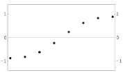
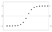
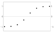
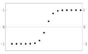
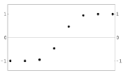
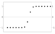
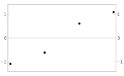
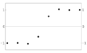
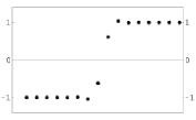
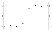
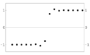
Figure 2: Numerical solutions for the scalar field configuration in the cases with $P_{4}$ for the left column, $P_{8}$ for the center column, and $P_{16}$ for the right column. Each vertical axis indicates $y_{i}=\phi_{i}/a$. The figures in the five rows correspond to the parameter $h=2^{-1},2^{-0.5},1,2^{0.5},2^{1}$, from the top to the bottom.

V.2 a soliton on a cycle graph

FIG. 3 shows the solitonic profile for $N=4,8,~{}{\rm and}~{}16$. The feature is the same as the case with the path graph.

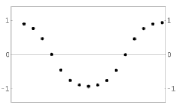
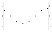
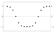
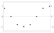
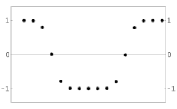
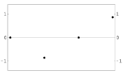
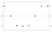
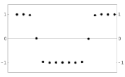
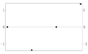
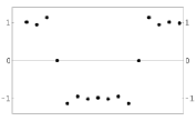
Figure 3: Numerical solutions for the scalar field configuration in the cases with $C_{4}$ for the left column, $C_{8}$ for the center column, and $C_{16}$ for the right column. Each vertical axis indicates $y_{i}=\phi_{i}/a$. The figures in the five rows correspond to the parameter $h=2^{-1},2^{-0.5},1,2^{0.5},2^{1}$, from the top to the bottom.

In both cases, a large $h$ means that the nonlinear part of the potential dominates the difference-square part. The tendency indicates that the simultaneous limit $N\rightarrow\infty$ and $h\rightarrow 0$ leads to the continuous solitons.

VI Yukawa couplings

Now we consider fermion fields coupled to the scalar fields. Our starting point is the discretization of the kinetic term in the continuum action in Sec. II. It is already known KS that the fermion kinetic term can be expressed in the incidence matrix ($E$). One set of chiral fermion fields $\psi$ are assigned on vertices of a graph and the other set of chiral fermion fields $\chi$ with the opposite chirality are assigned on edges of a graph. Then the discretized kinetic term has the form

$$-f\bar{\psi}E\chi+h.c.\,,$$

where indices are suppressed.

Now we postulate three possibilities of Yukawa interaction. We call them Case A, Case B, and Case C, for later convenience.

VI.1 a definition from difference operations

In the continuum theory, we have already seen that the scalar $(mass)^{2}$ matrix can be written in the form

$$\left|\frac{\partial W}{\partial\phi}\right|^{2}\,,$$ (28)

in the two-dimensional $\phi^{4}$ theory in Sec. II, while in our model,

$$\left|\frac{{\it\Delta}W}{{\it\Delta}\phi}\right|^{2}\,,$$ (29)

gives the potential, where

$$W(\phi_{i})=\frac{\phi_{i}^{3}}{3}-a^{2}\phi_{i}\,.$$ (30)

In the supersymmetric model, the fermion mass matrix is often given in the form

$$\frac{\partial^{2}W}{\partial\phi^{2}}\,,$$ (31)

in the continuum theory. The naive discretization of this form will be formally expressed as

$$\frac{{\it\Delta}^{2}W}{{\it\Delta}\phi^{2}}\,.$$ (32)

In actual, since ${\it\Delta}W/{\it\Delta}\phi$ is

$$g\left(\frac{\phi_{i+1}^{2}+\phi_{i+1}\phi_{i}+\phi_{i}^{2}}{3}-a^{2}\right)\,,$$ (33)

the difference of two sequential terms becomes

$$g\frac{\phi_{i+1}^{2}+\phi_{i+1}\phi_{i}-\phi_{i}\phi_{i-1}-\phi_{i-1}^{2}}{3}=g\frac{\phi_{i+1}+\phi_{i}+\phi_{i-1}}{3}(\phi_{i+1}-\phi_{i-1})\,,$$ (34)

$$= g\frac{\phi_{i+1}+\phi_{i}+\phi_{i-1}}{3}(\phi_{i+1}-\phi_{i}+\phi_{i}-\phi_{i-1})=g\frac{\phi_{i+1}+\phi_{i}+\phi_{i-1}}{3}({\it\Delta}\phi_{i}+{\it\Delta}\phi_{i-1})\,.$$

Graph theoretically speaking, the difference ${\it\Delta}\phi$ lives on each edge of a graph. Therefore we force chiral fermion fields on edges to couple the second difference in (34). Namely, for a cycle graph,

$${\tiny Y_{d}(C)=\frac{1}{3}\left(\begin{array}[]{cccccc}\phi_{N}+\phi_{1}+\phi_{2}&0&0&\cdots&0&\phi_{N}+\phi_{1}+\phi_{2}\\ \phi_{1}+\phi_{2}+\phi_{3}&\phi_{1}+\phi_{2}+\phi_{3}&0&\cdots&0&0\\ 0&\phi_{2}+\phi_{3}+\phi_{4}&\phi_{2}+\phi_{3}+\phi_{4}&\cdots&0&0\\ \vdots&\vdots&\vdots&\ddots&\vdots&\vdots\\ 0&0&0&\cdots&\phi_{N-2}+\phi_{N-1}+\phi_{N}&\phi_{N-2}+\phi_{N-1}+\phi_{N}\\ \phi_{N-1}+\phi_{N}+\phi_{1}&0&0&\cdots&0&\phi_{N-1}+\phi_{N}+\phi_{1}\end{array}\right)\,,}$$ (35)

couples to $\chi$ as $Y_{d}(C)\chi$, where

$$\chi=\left(\begin{array}[]{c}\chi_{1}\\ \chi_{2}\\ \vdots\\ \chi_{N}\end{array}\right)\,.$$ (36)

For a path graph, the coupling at both ends should be fixed by hand. We take

$${\tiny Y_{d}(P)=\frac{1}{3}\left(\begin{array}[]{cccccc}2\phi_{1}+\phi_{2}&0&0&\cdots&0&0\\ \phi_{1}+\phi_{2}+\phi_{3}&\phi_{1}+\phi_{2}+\phi_{3}&0&\cdots&0&0\\ 0&\phi_{2}+\phi_{3}+\phi_{4}&\phi_{2}+\phi_{3}+\phi_{4}&\cdots&0&0\\ \vdots&\vdots&\vdots&\ddots&\vdots&\vdots\\ 0&0&0&\cdots&\phi_{N-2}+\phi_{N-1}+\phi_{N}&\phi_{N-2}+\phi_{N-1}+\phi_{N}\\ 0&0&0&\cdots&0&\phi_{N-1}+2\phi_{N}\end{array}\right)}$$ (37)

which couples to $\chi$ as $Y_{d}(P)\chi$, where

$$\chi=\left(\begin{array}[]{c}\chi_{1}\\ \chi_{2}\\ \vdots\\ \chi_{N-1}\end{array}\right)\,.$$ (38)

We consider the four-dimensional fermion bilinear term

$$f\bar{\psi}(-E+h^{\prime}a^{-1}Y_{d})\chi+h.c.\,,$$ (39)

where $\psi=(\psi_{1},\psi_{2},\cdots,\psi_{N})$ is fermions on vertices of the opposite chirality to $\chi$. The coupling $h^{\prime}$ is $Ga/f$, where $G$ is the general Yukawa coupling.

VI.2 a definition from SUSY inspired structures

Suppose a cycle graph. The superpotential $W_{i}$ can be defined on each edge as

$$W_{i}([\phi],[\Phi])=[\Phi]_{i}\left[f([\phi]_{i+1}-[\phi]_{i})+g\left(\frac{[\phi]_{i+1}^{2}+[\phi]_{i+1}[\phi]_{i}+[\phi]_{i}^{2}}{3}-a^{2}\right)\right]\,,$$ (40)

where the superfields represent multiplets, each of which consists of a scalar, a chiral fermion, and an auxiliary field:

$$[\phi]_{i}\ni(\phi_{i},\psi_{i},F^{v}_{i})\,,$$ (41)

$$[\Phi]_{i}\ni(\Phi_{i},\chi_{i},F^{e}_{i})\,.$$ (42)

Then we get

$$\left(\frac{\partial W_{i}}{\partial\Phi_{i}}\right)^{2} = f^{2}(\phi_{i+1}-\phi_{i})^{2}+g^{2}\left(\frac{\phi_{i+1}^{2}+\phi_{i+1}\phi_{i}+\phi_{i}^{2}}{3}-a^{2}\right)^{2}$$ (43)

$$+2fg\left(\frac{\phi_{i+1}^{3}-\phi_{i}^{3}}{3}-a^{2}(\phi_{i+1}-\phi_{i})\right)\,.$$

Assuming $\Phi_{i}=0$, the potential for $\phi_{i}$ is given by

$$\sum_{i=1}^{N}\left(\frac{\partial W_{i}}{\partial\Phi_{i}}\right)^{2}=\sum_{i=1}^{N}\left[f^{2}(\phi_{i+1}-\phi_{i})^{2}+\left(\frac{\phi_{i+1}^{2}+\phi_{i+1}\phi_{i}+\phi_{i}^{2}}{3}-a^{2}\right)^{2}\right]\,,$$ (44)

since there is no terminal vertex in a cycle graph. This is just the scalar sector in our model considered in the present paper.

Thus we can derive the coupling terms from (40). The fermion bilinear term is found to be

$$\sum_{i}\bar{\chi}_{i}\left[f(\psi_{i+1}-\psi_{i})+g\frac{2\phi_{i+1}\psi_{i+1}+\phi_{i}\psi_{i+1}+\phi_{i+1}\psi_{i}+2\phi_{i}\psi_{i}}{3}\right]+h.c.\,.$$ (45)

Now we define

$${\small Y^{T}_{s}(C)=\frac{1}{3}\left(\begin{array}[]{cccccc}2\phi_{1}+\phi_{2}&\phi_{1}+2\phi_{2}&0&\cdots&0&0\\ 0&2\phi_{2}+\phi_{3}&\phi_{2}+2\phi_{3}&\cdots&0&0\\ \vdots&\vdots&\vdots&\ddots&\vdots&\vdots\\ 0&0&0&\cdots&2\phi_{N-1}+\phi_{N}&\phi_{N-1}+2\phi_{N}\\ \phi_{N}+2\phi_{1}&0&0&\cdots&0&2\phi_{N}+\phi_{1}\end{array}\right)\,,}$$ (46)

and rewrite the bilinear term as

$$f\bar{\chi}(-E^{T}+ha^{-1}Y_{s}^{T})\psi+h.c.\,.$$ (47)

The coupling $h$ may be changed to $h^{\prime}$ in a general case.

In the case with a path graph,

$${\small Y^{T}_{s}(P)=\frac{1}{3}\left(\begin{array}[]{cccccc}2\phi_{1}+\phi_{2}&\phi_{1}+2\phi_{2}&0&\cdots&0&0\\ 0&2\phi_{2}+\phi_{3}&\phi_{2}+2\phi_{3}&\cdots&0&0\\ \vdots&\vdots&\vdots&\ddots&\vdots&\vdots\\ 0&0&0&\cdots&2\phi_{N-1}+\phi_{N}&\phi_{N-1}+2\phi_{N}\end{array}\right)}$$ (48)

can be selected. Note in this case, although the terminal vertices may break an exact supersymmetry. Of course, supersymmetry is merely a guiding principle here.

VI.3 a definition from a simple democracy on edges and vertices

Another simple choice respecting a graph structure for the Yukawa couplings is possible. The definition is

$${\small Y^{T}_{e}(C)=\left(\begin{array}[]{cccccc}\phi_{1}&\phi_{2}&0&\cdots&0&0\\ 0&\phi_{2}&\phi_{3}&\cdots&0&0\\ \vdots&\vdots&\vdots&\ddots&\vdots&\vdots\\ 0&0&0&\cdots&\phi_{N-1}&\phi_{N}\\ \phi_{1}&0&0&\cdots&0&\phi_{N}\end{array}\right)\,,}$$ (49)

for a cycle graph and also

$${\small Y^{T}_{e}(P)=\left(\begin{array}[]{cccccc}\phi_{1}&\phi_{2}&0&\cdots&0&0\\ 0&\phi_{2}&\phi_{3}&\cdots&0&0\\ \vdots&\vdots&\vdots&\ddots&\vdots&\vdots\\ 0&0&0&\cdots&\phi_{N-1}&\phi_{N}\end{array}\right)}$$ (50)

for a path graph.

The four dimensional fermion bilinear term is

$$f\bar{\chi}(-E^{T}+h^{\prime}a^{-1}Y_{e}^{T})\psi\,.$$ (51)

We considered three cases for Yukawa couplings. In the next section, we will obtain the spectrum of the fermions for each case.

VII mass spectra for fermions and localization

FIG. 4 shows the fermion mass spectrum for the model associated with a path graph and that with a cycle graph. The eigenvalues of the matrix $(-E+ha^{-1}Y)(-E^{T}+ha^{-1}Y^{T})$ are plotted, where the suffices indicating definitions of the Yukawa coupling are suppressed. The Yukawa coupling constant is taken as $h^{\prime}=h$, so that the model in the continuum limit is expected to correspond with the supersymmetric model in Sec. II.

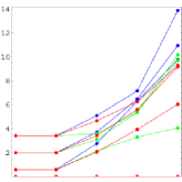
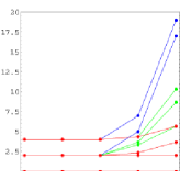
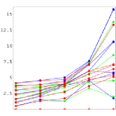
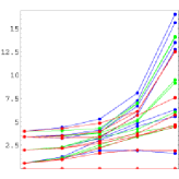
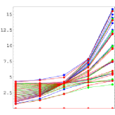
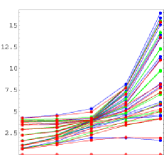
Figure 4: The spectra of the fermion mass-square in the case with a path graph for the left column and a cycle graph for the rught column. The figures in the three rows correspond to $N=4,8,16$, from the top to the bottom. The horizontal ticks correspond to the parameter $h=2^{-1},2^{-0.5},1,2^{0.5},2^{1}$, from the left to the right. The red points indicate the eigenvalues in Case A, the green points indicate the eigenvalues in Case B, while the blue points indicate the eigenvalues in Case C.

For the mode with a path graph $P_{16}$, we can see the degeneracy of eigenvalues at $h\sim 1$. In other cases, the degeneracy may occur at slightly large value for $h$.

It is known that the fermion spectrum has the finite discrete modes and continuous modes in the background of a kink in the continuum theory DJR . The degeneracy of our case reflects the continuum spectrum in the corresponding field theory. This phenomenon bring about for the appropriate coupling $h$, because the scalar configuration leaves far from the kink shape for small and large $h$. For a small $h$, the difference-squared part is dominant. For a large $h$, the non-linear potential is dominant. In both cases the shape of a kink is deformed.

Finally we show the localization of zero mode fields. In applications to the particle physics, the localization of matter fields is expected and is substantial for inclusion of other interactions among the matter fields dw ; ex . In FIG. 5, the eigenvectors associated with zero eigenvalues for $P_{16}$ with $h=1$ are exhibited.

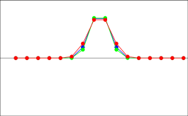
Figure 5: The profiles of the eigenvectors associated with zero modes for $P_{16}$ with $h=1$. The red points indicate the eigenmodes in Case A, the green points indicate the eigenmodes in Case B, while the blue points indicate the eigenmodes in Case C.

The difference of profiles of zero modes is minute for the three choices for the Yukawa couplings. As in the model with a continuous extra dimension, we can utilize the ‘localization’ for constructing elaborated gauge interacting models with several gauge groups.

VIII Summary and outlook

We investigated the solitonic configuration of scalar fields in deconstructed theory, or in a discrete extra space. It is expected that a large number of fields realizes the thee configuration corresponding to the kink in the continuum space.

We found discrete eigenvalues for fermions appropriately coupled to the kink-like configuration of scalar fields and the appearance of degeneracy of them for a set of certain critical couplings. This degeneracy is not observed in the continuum theory, where the continuum spectrum can be found. We also emphasis on the simple features of the models: the localization of matter fields occurs and the existence of zero modes, which correspond to the standard-model particles, is guaranteed.

The application of the deconstructed scalar model to particle physics turns to be interesting. The degeneracy in the spectrum may lead to the significant quantum effects on the zero mode fields if the other interactions are turned on. The difference from the higher-dimensional model with compactification is expected to be found, since the continuum theory includes infinite tower of fields. Moreover the study of the Casimir effect will be important especially if gravitation is incorporated into the models. We think that the dynamical creation and evolution of the kink or ‘topological’ (not in the strict meanings) configuration are worth studying in the cosmological context.

The generalization of models to those with the structure of general graphs other than cycle and path graphs is mathematically interesting. We wish also to investigate deconstructing non-linear sigma models and ‘topological’ configurations in them in the future works.

References

• (1) K. Akama, Gauge Theory and Gravitation, Proceedings of the International Symposium, Nara, Japan, 1982, ed. K. Kikkawa, N. Nakanishi and H. Nariai (Springer-Verlag, 1983), p. 267. V. Rubakov and M. Shaposhnikov, Phys. Lett. B125 (1983) 139.
• (2) M. Sakamoto, M. Tachibana, and K. Takenaga, Phys. Lett. B457 (1999) 33. N. Arkani-hamed and M. Schmaltz, Phys. Rev. D61 (2000) 033005. E. A. Mirabelli and M. Schmaltz, Phys. Rev. D61 (2000) 113011. H. Georgi, A. K. Grant and G. Hailu, Phys. Rev. D63 (2001) 064027. B. Grzadkowski and M. Toharia, Nucl. Phys. B686 (2004) 165. H. T. Cho, Phys. Rev. D72 (2005) 065010. M. Toharia and M. Trodden, Phys. Rev. D77 (2008) 025029. R. Davies, D. P. George and R. R. Volkas, Phys. Rev. D77 (2008) 124038. B. D. Callen and R. R. Volkas, Phys. Rev. D83 (2011) 056004.
• (3) N. S. Manton and T. M. Samols, Phys. Lett. B207 (1988) 179. J.-Q. Liang, H. J. W. Müller-Kirsten, and D. H. Tchrakian, Phys. Lett. B282 (1992) 105. I. Bakas and C. Sourdis, Fortschr. Phys. 50 (2002) 815.
• (4) N. Arkani-hamed, A. G. Cohen, and H. Georgi, Phys. Lett. B513 (2001) 232; Phys. Rev. Lett. 86 (2001) 4757; C. T. Hill, S. Spokorski, and J. Wang, Phys. Rev. D64 (2001) 105005.
• (5) J. M. Speight and R. S. Ward, Nonlinearity 7 (1994) 475 [arXiv:patt-sol/9911008]; J. M. Speight, Nonlinearity 10 (1997) 1615 [arXiv:patt-sol/9703005]. F. Cooper, A. Khare, B. Mihaila, and A. Saxena, Phys. Rev. E72 (2005) 036605. S. V. Dmitriev, P. G. Kevrekidis, N. Yoshikawa, and D. J. Frantzeskakis, Phys. Rev. E74 (2006) 046609. I. Roy, S. V. Dmitriev, P. G. Kevrekidis, and A. Saxena, Phys. Rev. E76 (2007) 026601.
• (6) N. Kan and K. Shiraishi, J. Math. Phys. 46 (2005) 112301. N. Kan, K. Kobayashi and K. Shiraishi, Phys. Rev. D80 (2009) 045005.
• (7) For reviews, R. Rajaraman, “Solitons and Instantons” (North-Holland, Amsterdam, 1987). M. Shifman and A. Yung, “Supersymmetric Solitons” (Cambridge Univ. Press, New York, 2009).
• (8) R. F. Dashen, B. Hasslacher, and A. Neveu, Phys. Rev. D10 (1974) 4130. R. Jackiw and C. Rebbi, Phys. Rev. D13 (1976) 3398.
• (9) C. Godsil and G. Royle, Algebraic Graph Theory (2001) (NewYork: Springer). D. Cvetković, P. Rowlinson and S. Simić, An Introduction to the Theory of Graph Spectra (London Mathematical Society Student Texts vol 75) (2010) (Cambridge: Cambridge University Press).