Entanglement Spectra of the 2D AKLT Model: VBS/CFT Correspondence
Abstract
We investigate the entanglement properties of the valence-bond-solid (VBS) state defined on two-dimensional lattices, which is the exact ground state of the Affleck-Kennedy-Lieb-Tasaki model. It is shown that the entanglement entropy obeys an area law and the non-universal prefactor of the leading term is strictly less than . The analysis of entanglement spectra for various lattices reveals that the reduced density matrix associated with the VBS state is closely related to a thermal density matrix of a holographic spin chain, whose spectrum is reminiscent of that of the spin-1/2 Heisenberg chain. This correspondence is further supported by comparing the entanglement entropy in the holographic spin chain with conformal field theory predictions.
pacs:
75.10.Jm, 75.10.Kt, 05.30.-d, 03.67.MnI Introduction
There has been considerable recent interest in understanding quantum entanglement in many-body systems.Amico_review ; Eisert_review Entanglement (von Neumann) entropy and the family of Rényi entropies are often used to quantify the degree of entanglement of a bipartite system consisting of two subsystems and . However, as pointed out by Li and Haldane,Li_Haldane the entanglement spectrum (ES), the eigenvalue spectrum of the reduced density matrix (RDM) of either system or , provides a more complete description of the ground state and the low-energy states of the system. In general, the RDM for may be written as with the entanglement Hamiltonian . Li and Haldane demonstrated that the spectrum of for fractional quantum Hall states on a sphere reflects the gapless edge excitations in the disk geometry. Since then, the ES has been applied to other systems such as topologically ordered systems Lauchli_ES ; Thomale_ES ; Fidkowski_ES ; Qi_Katsura_Ludwig and quantum spin models,Calabrese_ES ; Pollmann_ES ; Poilblanc_ES ; Yao_Qi_ES and the entanglement gap was proposed as a non-local order in gapless spin chains.Thomale_spin_chain
Although the analysis of the ES has turned out to be a powerful tool to extract universal properties, the application has so far been limited to one-dimensional (1D) or topological systems. To fill this gap in the literature, we examine the ES in the two-dimensional (2D) quantum spin model proposed by Affleck, Kennedy, Lieb, and Tasaki (AKLT).AKLT The AKLT model in one dimension was first introduced as a solvable model to illustrate the Haldane-gap phase in integer spin chains. The exact ground state is known as the valence-bond-solid (VBS) state. The construction of the VBS state generalizes to two and higher dimensions.KLT ; Kirillov_Korepin The VBS state has recently attracted renewed interest from the viewpoint of quantum computation. It was proposed that VBS states on a 2D hexagonal lattice can serve as resources for measurement-based quantum computation.Wei_Affleck ; Miyake Thus, the study of the ES in VBS states on various 2D lattices can shed some light on this important issue.
In this paper, we study numerically the ES in the 2D AKLT model defined on various lattices. We develop an efficient way to evaluate the RDM using a Monte Carlo (MC) method. The ES is then obtained by numerical diagonalization. It is shown that the ES is not flat in 2D, which is in contrast to the 1D case where all eigenvalues of the RDM become degenerate in the thermodynamic limit. Xu_Katsura_Korepin_Hirano ; Korepin_Xu When a system is on a cylinder, we can study the ES as a function of momentum. The low-lying spectrum of the entanglement Hamiltonian for square (hexagonal) VBS state is reminiscent of that of the 1D antiferromagnetic (ferromagnetic) Heisenberg chain. This indicates that the entanglement Hamiltonian is very close to the Heisenberg Hamiltonian in one dimension. To further support this idea, we introduce a new concept, nested entanglement entropy (NEE), and find that, for the square lattice VBS state, the low-energy effective Hamiltonian of is well described by conformal field theory (CFT) despite that the starting quantum state (the AKLT state in this paper) is not critical. For a hybrid system consisting of squares and hexagons, we find that the ES is gapped and is close to the alternating Heisenberg chain in which ferromagnetic and antiferromagnetic interactions are mixed.
The organization of the rest of the paper is as follows. In Sec. II, we first review the construction of the VBS ground states on two-dimensional lattices. We then show how to obtain the spectrum of RDM from the Schmidt decomposition of the VBS state. We see that the Schmidt coefficients are related to the eigenvalues of the overlap matrix (see Eq. (6) for the precise definition). In Sec. III, we show numerical results of entanglement entropy and spectrum of the VBS states on both square and hexagonal lattices. We then introduce the NEE and study its scaling properties. We also present an example of the gapped entanglement spectrum, which is obtained from the VBS state on the hybrid lattice consisting of squares and hexagons. We conclude with a summary in Sec. IV. Analytical and numerical approaches for obtaining the overlap matrix are, respectively, presented in Appendices A and B.
II 2D VBS states
II.1 AKLT Hamiltonian
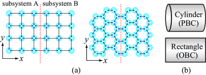
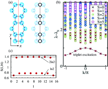
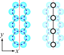
We study the AKLT model on the square and hexagonal lattices shown in Fig. 1 (a). For simplicity, we focus on the basic model in which there is a single valence bond on each edge. The spin- Hamiltonian for this model is written as a sum of projection operators as
| (1) |
where is an arbitrary positive number and projects the total spin of each pair of neighboring spins onto the subspace of . The spin magnitude and the coordination number are related through , where for the square lattice, while for the hexagonal lattice. The unique ground state (VBS state) of is written as
| (2) |
where and are Schwinger bosons at site , satisfying
| (3) |
with all other commutators vanishing, and denotes the vacuum state.Arovas_Auerbach_Haldane With the constraint that the total number of bosons at each site is , the original spin operators can be represented by the Schwinger bosons as
| (4) |
We will study VBS states defined on lattices with both periodic (PBC; cylindrical geometry) and open (OBC; rectangular geometry) boundary conditionsfootnote:boundary shown in Fig. 1 (b).
II.2 Reduced density matrix
Let us consider a bipartition into two subsystems and , each of which is a mirror image of the other, and the boundary between them is chosen to be the reflection axis. We denote the bulk width of () by and the number of bonds on the boundary by . The Hamiltonian can be written in the form where and denote the Hamiltonians within subsystems and , respectively, while contains all the interactions across the boundary. The RDM for describing the entanglement between the two subsystems is defined by , where . To obtain the spectrum of , we follow the same approach used in Ref. KKKKT, . The ground state of the system can be written as
| (5) |
where and () is a set of degenerate ground states of (), each of which is characterized by a configuration of bosons at the boundary sites. These states are linearly independent but not orthogonal. We now introduce overlap matrices as
| (6) |
for two subsystems, respectively. Due to the reflection symmetry, one can show that and is real symmetric and positive definite. One can then construct the orthonormal states out of () using an orthogonal matrix that diagonalizes , i.e., :
| (7) |
The ground state of the full system in the new basis is written in the Schmidt decomposition as
| (8) |
and hence . Therefore, the spectrum of is equivalent to that of the following matrix
| (9) |
where denotes the standard matrix trace (not to be confused with ). One can regard as a thermal density matrix of an auxiliary spin chain, which we call a holographic spin chain. The notion of this hidden spin chain was first introduced in Ref. KKKKT, . The entanglement Hamiltonian is defined via .
We can obtain the overlap matrix analytically for VBS states defined on vertical ladders (i.e. ) (see Appendix A). For VBS states on lattices with a larger width (), in which case results converge to the 2D limit, we develop an efficient algorithm of MC method (see Appendix B for details). We sample all possible configurations of bosons stochastically, and each matrix element can be numerically obtained as the accumulation number of states.
III Entanglement entropy, spectrum, and nested entanglement entropy
In this section, we show the results of entanglement entropy and spectrum for the VBS states obtained by the MC method combined with exact diagonalization. As we will show, the ES of the square (hexagonal) VBS state resembles the energy spectrum of the antiferromagnetic (ferromagnetic) Heisenberg Hamiltonian in one dimension. We also introduce a new quantity, nested entanglement entropy, and further elucidate the relationship between the holographic spin chain and the Hamiltonian for the Heisenberg chain.
III.1 Entanglement entropy
Let us first study the entanglement entropy (EE) which can be obtained from
| (10) |
where () are the eigenvalues of .
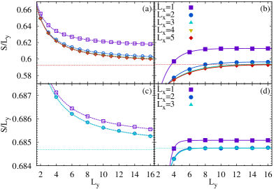
The obtained EE divided by the boundary length for the square and hexagonal lattices are shown in Fig. 2. In both cases, we investigate lattices with both PBC and OBC, results of which are expected to be equivalent in the thermodynamic limit (). The EE per unit boundary length in 2D AKLT model is found to be strictly less than , which is in contrast to the result for the 1D AKLT model.Fan_Korepin ; Xu_Katsura_Korepin_Hirano ; Korepin_Xu Note that the area law is satisfied, as approaches to a constant in the thermodynamic limit.
The difference between 1D and 2D EE results can be understood in terms of “valence bond loops” (VBL), which are formed by sequences of singlets connected head-to-tail. (A precise definition of VBL in the context of Schwinger boson can be found in Appendix B.) The existence of such loops is a unique feature of 2D VBS states, which provides additional correlations between two separated singlets. As a result, we expect extra correlations between boundary bosons in the 2D VBS states, which lead to modification of the EE from the 1D result. The possibility of forming a valence bond loop decays exponentially fast with respect to its length. (The reason is discussed in Appendix B). This can be related to multiple observed pheonomena of EE from our numerical calculation.
First of all, in VBS states on the square lattice, the magnitude of deviation from the 1D result () is significantly larger than that of the hexagonal lattice. To understand this, we observe that elemental loops (shortest VBLs that have largest possibility) connects two boundary sites directly in the square lattice, while an extra site is in between two boundary spins in the hexagonal lattice. As a result, the amplitude of elemental loops is higher in the square lattice. In the end, we obtain considerably more VBLs, which then induce larger amount of extra correlations on the boundary in the square lattice than in the hexagonal lattice.
Meanwhile, increasing the number of sites in the bulk direction provides additional valence bond loops which involve sites not only on the boundary, but also inside the two-dimensional lattice. Hence the EE is further reduced when expanding bulk width . The effect converges exponentially fast, however. The 2D limit has been almost reached at and for square and hexagonal VBS states, respectively. It is again related to the fact that the amplitude of a VBL decreases with its length.
We also observe that the thermodynamic limit () of EE is achieved with totally different behaviors for lattices with rectangular (OBC) and cylindrical (PBC) geometries, as shown in Fig. 2. For VBS states on a lattice with OBC, is found to scale with the boundary length () as
| (11) |
where are the fitting parameters and denotes the EE per boundary length in the thermodynamic limit. The magnitude of is significantly less than , as shown in Table 1. In contrast, for a lattice wrapped on a cylinder (PBC), the thermodynamic limit is approached exponentially fast in , i.e., , where (also shown in the table) is of the order of the lattice spacing.
| square | |||||
|---|---|---|---|---|---|
| OBC | PBC | ||||
| hexagonal | |||||
|---|---|---|---|---|---|
| OBC | PBC | ||||
Such distinctively different behaviors of EE for PBC and OBC lattices are closely related to VBL formations. For example, for the square lattice the leading correction to boundary spin correlations and EE is associated with a group of elemental valence bond loops mentioned above, each connecting two nearest neighbor boundary spins. In a lattice with rectangular geometry (OBC), the number of such elemental loops is always less than the number of boundary sites . As a result, the leading correction to entropy per boundary spin is proportional to , which approaches in the thermodynamic limit. Accordingly, we expect that the entanglement entropy converges slowly following the function , as observed in Fig. 2.
For a lattice wrapped on a cylinder (PBC), winding loops associated with periodic boundary provide extra spin-spin correlations to the system. The EE in a finite system is lower than the result in the thermodynamic limit, due to the fact that such winding valence bond loops are more prominent in a smaller lattice compared with those in a larger one. Furthermore, amplitudes associated with winding loops decay exponentially fast according to the number of boundary spins , which is of the same order of winding loops’ length. As a result, we observe a exponentially converging behavior of the entanglement entropy in a PBC lattice.
III.2 Entanglement spectrum
Let us now consider the ES defined as a set of eigenvalues of the entanglement Hamiltonian . In a system with PBC, we are able to study the ES as a function of momentum in the -direction ( in Fig. 3).
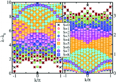
As shown in Fig. 3, the ES obtained from the square (hexagonal) VBS states resembles the spectrum of the spin-1/2 antiferromagnetic (ferromagnetic) Heisenberg chain. The reason for the dependence of the ES on the lattice structure is as follows: Although both the square and hexagonal lattices are bipartite, neighboring boundary spins belong to the different sublattices in the case of the square VBS state. As a result, the entanglement Hamiltonian is reminiscent of the AFM Heisenberg chain. In contrast, in the hexagonal lattice, all boundary spins belong to the same sublattice, hence the FM spectrum appears. The lowest-lying modes in the left panel can be identified as the des Cloizeaux-Pearson spectrum in the AFM Heisenberg chain desCloizeaux_Pearson . In the right panel, the excitations with the total spin look like the ordinary spin-wave spectrum in the FM Heisenberg chain. In fact, due to the translational symmetry in the direction, the Bloch theorem applies and the single-magnon states in the FM chain are exact eigenstates of the RDM for the hexagonal VBS state.
III.3 Nested entanglement entropy
In order to further establish the correspondence between the holographic spin chain and the Hamiltonian for the Heisenberg chain, we introduce a measure, which we call nested entanglement entropy (NEE), and study its scaling properties. One might think that the finite-size scaling analysis of the ground state energy is sufficient to reveal the CFT structure in the holographic spin chain. However, there is a subtle point here. The spectrum of the RDM can only tell us that the entanglement Hamiltonian can be expressed as with the Hamiltonian for the holographic chain . There is no unique way to disentangle a fictitious temperature from . Assuming that is gapless and its low-energy dispersion is given by , we can estimate from the slope of the modes at in the left panel of Fig. 3 (see Table 2). The obtained slope shows saturation at about , which suggests that the fictitious temperature is presumably nonzero () in the infinite 2D system. As we will see, however, the NEE provides a more clear-cut approach to investigate the critical behavior of without any assumption.
Let us now give a precise definition of the NEE. Based on the ground state of the entanglement Hamiltonian , we construct the nested RDM for the sub-chain of length in the holographic spin chain as
| (12) |
where denotes the normalized ground state of and the trace is taken over the remaining sites excluding the sub-chain. The NEE is then obtained from the nested RDM as
| (13) |
where the trace is over the sites on the sub-chain. Since the low-energy physics of the AFM Heisenberg chain is described by CFT, the NEE is expected to behave as Calabrese_Cardy
| (14) | |||||
| (15) |
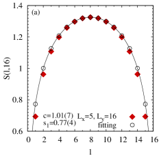
for a lattice with PBC, where is the central charge, and is a non-universal constant. In Fig. 4 (a), we show NEE obtained from the square VBS state with and . The CFT prediction, Eq. (14), well explains the spatial profile of the NEE. The fit yields which is reasonably close to .
The NEE for (half-NEE) is simplified to be
From the data with the finite-size scaling form of the NEE, we can also extract the central charge as summarized in Table 3.
For the case , is remarkably close to unity. This further supports our conjecture: a correspondence between the entanglement Hamiltonian of the 2D AKLT model and the physical Hamiltonian of the 1D Heisenberg chain. A slight modification of is observed as the bulk width increases from to .
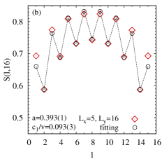
In the case of the rectangular geometry (OBC), a staggered pattern of NEE is expected from studies of the standard EE in open spin chains Laflorencie_et_al ; Hikihara_et_al :
| (16) |
In Fig. 4 (b), we show the NEE for the square VBS state on the rectangle with and . We take the central charge to be and the Tomonaga-Luttinger parameter , and tune and as fitting parameters. The fit is reasonably good except for the boundaries. This deviation might be due to logarithmic corrections which appear in the SU(2) symmetric AFM spin chains Laflorencie_et_al but are not taken into account in Eq. (16).
To provide further evidence for the holographic spin chain, we now consider the hybrid system comprised of squares and hexagons, shown in Fig. 5(a). It is expected that the entanglement Hamiltonian is described by the FM-AFM alternating Heisenberg model. Figure 5(b) shows the ES for this system. It is clearly seen that there is a gap between the ground state and the continuum. The gap rapidly saturates with increasing . The behavior of the ES is totally consistent with the energy spectrum of the alternating Heisenberg chain whose interactions are denoted and .Hida_alternating Comparing the bound-state spectrum in Fig. 5(b) with that of the triplet-pair excitation in the alternating Heisenberg chain,Hida_alternating we estimate the ratio of the FM exchange divided by the AFM one as . Note that one can further manipulate of the holographic spin chain by tuning the lattice structure and the number of valence bonds on each edge the lattice. The NEE associated with the ground state of is shown in Fig. 5(c). The NEE is when two AFM bonds are cut, whereas it becomes about when both FM and AFM bonds are cut. The obtained result is in good agreement with the standard EE in the alternating Heisenberg chain studied in Ref. Hirano-Hatsugai, .
IV Conclusion
We have studied both the entanglement entropy and spectrum associated with the VBS ground state of the AKLT model on various 2D lattices. It was shown that the reduced density matrix of a subsystem can be interpreted as a thermal density matrix of the holographic spin chain, whose spectrum resembles that of the spin-1/2 Heisenberg chain. To elucidate this relationship, we have introduced the concept, nested entanglement entropy (NEE), which allows us to clarify this correspondence in a quantitative way without information on the fictitious temperatures. The finite-size scaling analysis of the NEE revealed that the low-energy physics of the holographic chain associated with the square lattice VBS is well described by conformal field theory. The NEE was also applied to the hybrid VBS state, the entanglement spectrum of which is gapped, and the holographic chain was found to be the alternating Heisenberg chain.
Acknowledgment
The authors thank Toshiya Hikihara, Vladimir E. Korepin, Takafumi Suzuki, and Hal Tasaki for valuable discussions, and Hidetoshi Nishimori for TITPACK, ver. 2. This work was supported by Grant-in-Aid for JSPS Fellows (23-7601), for Young Scientists (B) (23740298), for Scientific Research (B) (22340111), and for Scientific Research on Priority Areas (19052004). Numerical calculations were performed on supercomputers at the Institute for Solid State Physics, University of Tokyo.
Note added.— While completing this work, we became aware of a paper by I. J. Cirac et al. Cirac_et_al in which similar results were obtained using different approaches.
Appendix A Analytical method for
In this appendix, we show how to explicitly calculate the reduced density matrix for ladders with OBC and PBC based on an extension of the method described in Ref. KKKKT, , in which the authors analytically obtained entanglement entropies of the VBS states with OBC using a transfer matrix technique. According to Ref. KKKKT, , the overlap matrix for vertical ladder, i.e. is given by
| (17) |
where denotes the coordination number at the -th site, is the unit vector defined by , and is the Pauli matrix vector. For PBC, . The above expression for can be derived using the Schwinger boson representation and coherent state representation. It is convenient to introduce -matrix defined by
| (18) | |||||
Since the only difference between and is the overall factor, the spectrum of is equivalent to that of the following matrix:
| (19) |
where is taken over -spin spaces. Then in order to calculate entanglement properties of the VBS state on a vertical ladder, it is necessary to obtain the explicit form of -matrix. There is a useful relation shown in lemma 3.3 in Ref. KLT, :
| (20) |
where . Using the above relation we obtain the following relation:
| (21) | |||||
where and . The summation is taken over admissible combinations of for . It is useful to express Eq. (21) in terms of graphical representations.
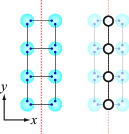
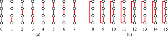
Figure 6 shows the relationship between the original VBS state and the one-dimensional holographic spin chain. The circles in the right panel in Fig. 6 indicate the sites in the spin chain, on which the Pauli vectors in Eq. (21) act. -matrix is represented by sum of admissible configurations each of which has a corresponding graph (see Fig. 7). Here the number of admissible configurations is .
Let us consider the case for illustrative purposes. Figure 7(a) shows all admissible configurations for OBC using a bit representation in which the thin and thick lines denote and , respectively. The end points of thick lines in Fig. 7 indicate .
For example, the contributions of the states 3 and 5 to the -matrix are expressed as
| (22) | |||
| (23) |
respectively. Note that in Eq. (21) corresponds to the number of clusters connected by thick lines contiguously in each graphical representation. Summing all contributions, we arrive at the following expression for the -matrix:
| (24) | |||||
where is a -dimensional identity matrix.
Next, we examine the case of PBC where the number of admissible configurations is . We have to consider the states depicted in Fig. 7 (b) in addition to the states in Fig. 7 (a). For example, contribution of the state 11 to the -matrix is given as
| (25) |
Including additional contributions from the states from to in Fig. 7 (b), the -matrix for PBC is given as
| (26) | |||||
In principle, we can obtain an explicit form of the -matrix for larger using the method based on the graphical representations.
Next we show how to calculate the -matrices for hexagonal-lattice vertical ladders (i.e. ). The relationship between the VBS on the hexagonal-lattice vertical ladder and the holographic spin chain is shown in Fig. 8.
The only difference between the square and hexagonal vertical ladders is the definition of the length between sites on the holographic spin chain. We can then calculate the -matrix for the hexagonal-lattice vertical ladder as follows:
| (27) | |||||
where and . The difference between Eq. (21) and Eq. (27) is an exponent of .
After we obtain an explicit form of -matrix, we can study entanglement properties. Indeed, we have compared the results based on this method with those obtained by Monte Carlo method and have confirmed that they are completely consistent, which ensures the validity of our Monte Carlo approach.
Appendix B Monte Carlo Method for Calculating Overlap Matrix
In this appendix, we explain our proposed Monte Carlo method used for obtaining the overlap matrix . As we mentioned in Sec. II, the VBS state can be regarded as a singlet-covering state, expressed by Eq. (2). In the case of bipartite lattices (square and hexagonal), we can avoid negative signs by a local gauge transformation:
| (28) |
where and denote the two sublattices. The VBS state can then be represented as
| (29) |
where runs over all connected neighboring sites in the graph. If we introduce as the quantum number of SU(2) boson operators, the VBS state can be written as
| (30) |
where denotes the boson between -th and -th site on the bulk of the subsystem . As a result, we can reproduce VBS state through stochastic sampling of boson configurations of the system.
The element of overlap matrix , is given by
| (31) |
where is the VBS state with fixed boundary :
| (32) | |||||
where denotes the boundary of . The variables specifies the unpaired spins on the boundary. We can further simplify the problem by considering (32) in the occupation number basis:
| (33) |
where (the summation is taken over all nearest neighbor sites of ) is the number of bosons of type at the site . The degeneracy of occupation number state can be easily derived as:
| (34) |
As a result, we obtain the element of the overlap matrix as
with weight
| (36) |
In the end, by generating boson states stochastically while keeping the constraint for all and , we can numerically calculate the element of the overlap matrix as accumulation number of boson configurations with corresponding boundary condition, through Monte Carlo importance sampling.
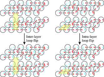
It is convenient to introduce graphical representation for each boson configurations , as shown in Fig. 9. The red (dark) and blue (light) lines indicate bosons with quantum number and , respectively. Colored but unconnected dots on the edge correspond to boundary bosons . Notice that we show two layers in the graphical representation, as they stand for the sub-system state and its conjugate , respectively. Due to the fact that the full system is reflection symmetric, one may also consider two layers as two subsystems A and B, with sites (big circles) and bonds (lines) on top of each other being symmetric counterparts.
Using this graphical representation, we can easily illustrate two MC update schemes we use to sample all possible boson configurations, while automatically satisfying the constrain: for all and .
(i)Inter-layer flip (Left panel of Fig. 9): In the boson state , we choose arbitrarily a valence bond connecting sites and such that (colored as red/blue) is satisfied. A trial state is given as (colored as blue/red) with all other bosons unchanged. The update is accepted/rejected according to the ratio of probabilities which satisfies detailed-balance condition. In Fig. 9, a yellow loop is drawn showing bosons being flipped ().
(ii)Intra-layer flip (Right panel of Fig. 9): In order to apply intra-layer flip without violating the constraints, we attempt to construct a “valence bond loop” (VBL), or a sequence of connected singlets, with alternating colors (). Flipping a VBL is equivalent to operating
| (37) |
on the VBS state (except for the weight change), where the loop is formed by sites in the order of , and are the alternating colors along the loop. (from red to blue and vice versa). In the right column of Fig. 9, we show a possible loop that consists of 4 sites and 4 valence bonds, denoted by yellow region. In our MC simulation scheme, we construct a loop by using a random walker. The walker starts from a randomly chosen site, as well as a randomly chosen direction. After such a movement, we choose next direction so that the color of next valence bond alternates. Since turning back to the previous site is in the list of candidates, it is always possible to choose such a direction. When the walker comes back to the initial position, the loop is formed. Therefore, loops can be of arbitary length, as long as color is alternating along the loop. Meanwhile, the possibility (amplitude) decrease significantly for longer loops. Nevertheless, obviously, flipping all the bonds in a valence bond loop does not affect the occupation number at any site on the loop.
Following above two updating rules, we can obtain efficiently the overlap matrix with high accuracy, while satisfying the ergodicity condition. This MC sampling approach can be applied to arbitrarily large systems. Number of sites along the bulk dimension has limited effect on the cost of calculations. The computational limit is mainly related to the diagonalization of the overlap matrix, the dimension of which grows exponentially as the number of boundary sites increases.
References
- (1) L. Amico, R. Fazio, A. Osterloh, and V. Vedral, Rev. Mod. Phys. 80, 517 (2008).
- (2) J. Eisert, M. Cramer, and M. B. Plenio, Rev. Mod. Phys. 82, 277 (2010).
- (3) H. Li and F. D. M. Haldane, Phys. Rev. Lett. 101, 010504 (2008).
- (4) A. M. Lauchli, E. J. Bergholtz, J. Suorsa, and M. Haque, Phys. Rev. Lett. 104, 156404 (2010).
- (5) R. Thomale, A. Sterdyniak, N. Regnault, and B. A. Bernevig, Phys. Rev. Lett. 104, 180502 (2010).
- (6) L. Fidkowski, Phys. Rev. Lett. 104, 130502 (2010).
- (7) X-L. Qi, H. Katsura, and A. W. W. Ludwig, arXiv:1103.5437v1 [cond-mat.mes-hall].
- (8) P. Calabrese and A. Lefevre, Phys. Rev A 78, 032329 (2008).
- (9) F. Pollmann, A. M. Turner, E. Berg, and M. Oshikawa, Phys. Rev. B 81, 064439 (2010).
- (10) D. Poilblanc, Phys. Rev. Lett. 105, 077202 (2010).
- (11) H. Yao and X-L. Qi, Phys. Rev. Lett. 105, 080501 (2010).
- (12) R. Thomale, D. P. Arovas, and B. A. Bernevig Phys. Rev. Lett. 105, 116805 (2010).
- (13) I. Affleck, T. Kennedy, E. H. Lieb, and H. Tasaki, Phys. Rev. Lett. 59, 799 (1987); I. Affleck, T. Kennedy, E. H. Lieb, and H. Tasaki, Commun. Math. Phys. 115, 477 (1988).
- (14) T. Kennedy, E. H. Lieb, and H. Tasaki, J. Stat. Phys. 53, 383 (1988).
- (15) A. N. Kirillov and V. E. Korepin, Algebra i Analiz. 1, 47 (1989); [St. Petersburg Math. J. 1, 343 (1990)].
- (16) T-C. Wei, I. Affleck, and R. Raussendorf, Phys. Rev. Lett. 106, 070501 (2011).
- (17) A. Miyake, Ann. Phys. 326, 1656 (2011).
- (18) Y. Xu, H. Katsura, T. Hirano, V. E. Korepin, J. Stat. Phys. 133, 347 (2008).
- (19) V. E. Korepin and Y. Xu, Int. J. Mod. Phys. B, 24, 1361 (2010).
- (20) D. Arovas, A. Auerbach, and F. D. M. Haldane, Phys. Rev. Lett. 60, 531 (1988).
- (21) Spins at the boundary sites have a different spin magnitude that is less than the bulk one ().
- (22) H. Katsura, N. Kawashima, A. N. Kirillov, V. E. Korepin, and S. Tanaka, J. Phys. A: Math. Theor. 43, 255303 (2010).
- (23) H. Fan, V. E. Korepin, and V. Roychowdhury, Phys. Rev. Lett. 93, 227203 (2004).
- (24) J. des Cloizeaux and J. J. Pearson, Phys. Rev. 128, 2131 (1962).
- (25) P. Calabrese and J. Cardy, J. Stat. Mech. P06002 (2004).
- (26) N. Laflorencie, E. S. Sorensen, M-S. Chang, and Ian Affleck, Phys. Rev. Lett. 96, 100603 (2006).
- (27) T. Hikihara, S. Lukyanov, and A. Furusaki (private communication).
- (28) K. Hida, J. Phys. Soc. Jpn. 63, 2514 (1994).
- (29) T. Hirano and Y. Hatsugai, J. Phys. Soc. Jpn. 76, 074603 (2007).
- (30) J. I. Cirac, D. Poilblanc, N. Schuch, and F. Verstraete, Phys. Rev. B 83, 245134 (2011).