The Kuramoto Model with Time-Varying Parameters

Abstract

We analyze the Kuramoto model generalized by explicit consideration of deterministically time-varying parameters. The oscillators’ natural frequencies and/or couplings are influenced by external forces with constant or distributed strengths. A new dynamics of the collective rhythms is observed, consisting of the external system superimposed on the autonomous one, a characteristic feature of many thermodynamically open systems. This deterministic, stable, continuously time-dependent, collective behaviour is fully described, and the external impact to the original system is defined in both, the adiabatic and non-adiabatic limits.

I Introduction

Biological examples provided the original motivation lying behind the Kuramoto model (KM) of coupled phase oscillators Strogatz_sync . However, neither the original model Kuramoto_book , nor any of its extensions Acebron_review , have incorporated a fundamental property of living systems – their inherent time-variability. Many important characteristics of open systems can be missed by not accounting for the non-equilibrium dynamics that stems from their time-dependent (TD) parameters. Additionally, the application of the KM to many problems would move closer to reality by allowing for the natural frequency of each oscillator, or the coupling strengths, to be externally modulated by TD forcing, as commonly occurs in living systems. Among the numerous collective rhythms traceable back to TD parameters, are frequency flows in brain signals Rudrauf , the modeling of brain dynamics under anaesthesia Jane1 where anaesthetic strength modulates natural frequencies Musizza , event-related oscillatory responses of the brain Pfurtschelle:99 , and the dynamics of cardiovascular ageing yuri10 . None of these are adequately described by existing models. Additionally, similar considerations are to be expected in non-biological examples such as pattern formation in a nonlinear medium far from equilibrium Lee2011 . Here, using trapped ions, one can vary the parameters at will and see the effect on the synchronization.

There has already been much work on coupled oscillators influenced by noise as a special form of external dynamics Strogatz2 . Likewise, driving by an external periodic force Shinomoto is a long-explored model, characterized by the interplay to the phases of each oscillator between the external pacemaker and the mean field of all other oscillators. A generalization of the KM that allowed certain time-varying frequencies and couplings was also numerically explored in Cumin2007 . However, the simulations were performed over a very small number of oscillators, the dynamics were not described analytically, and a qualitative description was not given for slow or fast varying cases. Other studies of non-constant collective rhythms include asymmetrically-coupled ensembles Montbrio and populations with multimodally distributed natural frequencies Bonilla1992 , with their complex mean field being a result of multimodal distribution of the parameters. Frequency adaptation as discussed in Taylor2010 assumes non-constant natural frequencies, but without external influence. It is similar to the models with inertia Acebron_inertia and its dynamics, apart from the stable incoherence, are characterized by either synchronization or bistable regime of both synchronized and incoherent states. In addition, the model with drifting frequencies Rougemont assumes frequency dynamics formulated as an Ornstein-Uhlenbeck process, but it also leads to time-independent mean fields, resembling the simple KM under influence of colored noise. Alternately-switching connectivity So2008 or periodic couplings Lee2012 , are some of examples with varying coupling strengths. Yet, most of the discussions in these are concerned with the networks and graph theory properties of the system, and only Heaviside step functions are considered for the interaction between oscillators.

Nevertheless, the TD mean fields in most of these models result either from multistability or from unstable equilibria. Despite this, even in the cases where it stems from some external system Cumin2007 ; So2008 ; Lee2012 , the low-dimensional mean field dynamics and slow/fast reduced approaches are still missing. As such, none of these models can fully demonstrate the deterministic and stable TD dynamics of many real physical, chemical, biological, or social systems that can never be completely isolated from their surroundings. These systems do not reach equilibrium but, instead, exhibit complex dynamical behavior that includes the TD frequencies and couplings. We will show that our generalization of the Kuramoto model encompasses these dynamics.

II Model

An external, explicitly time-dependent, bounded function $x(t)$ is introduced. It modulates the frequencies or couplings of the original model. This external influence can also originate from another Jane:11 non-constant mean field. In the most general case, the strengths of the interactions $I_{i}$ are distributed according to a probability density function (PDF) $h(I)$, and likewise the distribution $g(\omega)$ of the natural frequencies $\omega_{i}$. Thus, depending on which parameter is influenced two generalized Kuramoto models emerge

$$A :\ \ \ \dot{\theta}_{i}=\omega_{i}+I_{i}x(t)+K\ r(t)\sin[\psi(t)-\theta_{i}],$$ (1)

$$B :\ \ \ \dot{\theta}_{i}=\omega_{i}+[K+I_{i}x(t)]\ r(t)\sin[\psi(t)-\theta_{i}].$$ (2)

Here, a TD complex order parameter is introduced

$$z(t)=r(t)\mathrm{e}^{i\psi(t)}=\frac{1}{N}\sum_{j=1}^{N}\mathrm{e}^{i\theta_{j}},$$ (3)

where $r(t)$ and $\psi(t)$ are the TD mean-field amplitude and phase respectively. For clarity, their explicit time-dependence will henceforth be omitted.

For each oscillator at any given time there is 1:1 correspondence between the fixed and TD parameters, i.e.

$$\tilde{\omega}_{i}(t)=\omega_{i}+I_{i}x(t)$$

for model A, and

$$\tilde{K}_{i}(t)=K+I_{i}x(t)$$

for model B, or in general

$$\tilde{I}_{i}(t)=I_{i}x(t).$$

Thus, for known forcing $x(t)$, a single oscillator from both NA models can be uniquely defined by fixed parameters $\omega_{i}$ and $I_{i}$, or by the TD natural frequencies for the model A and TD couplings for model B, $\tilde{\omega}_{i}$ and $\tilde{K}_{i}$ respectively, which in this case also encompass $x(t)$. Similarly, instead of $\tilde{\omega}_{i}$ and $\tilde{K}_{i}$, $\omega_{i}$ and $\tilde{I}_{i}$ can be used, whereas distributions of these TD variables accordingly become $\tilde{g}(\tilde{\omega})$, $\tilde{\Gamma}(\tilde{K})$ and $\tilde{h}(\tilde{I})$.

To analyze the models (1), (2) the thermodynamic limit $N\rightarrow\infty$ is assumed. Here, the state of the system with fixed forcing ($x(t)=const.$) would have been described by a continuous PDF $\rho(\theta,\omega,I,t)$ which gives the proportion of oscillators with phase $\theta$ at time $t$, for fixed $\omega$ and $I$ Mirollo2007 . On the other hand, the one to one correspondence between the fixed and TD parameters in terms of PDFs implies that the same number of oscillators can be described by either of the following PDFs

$$|h(I)dI|=|\tilde{h}(\tilde{I}(I,t))\ d\tilde{I}|,$$ (4)

or

$$|g(\omega)d\omega|=|\tilde{g}(\tilde{\omega}(\omega,I,t))d\tilde{\omega}|$$

and

$$|\Gamma(K,I)dK|=|\tilde{\Gamma}(\tilde{K}(K,I,t))d\tilde{K}|$$

if $\tilde{\omega}$ and $\tilde{K}$ are used for describing the population. Also, the infinitesimal number of oscillators $dN$ is given by

$$dN = |\rho(\theta,\omega,I,t)\ g(\omega)\ h(I)\ d\theta\ d\omega\ dI|=$$ (5)

$$|\tilde{\rho}(\theta,\omega,\tilde{I},t)\ g(\omega)\ \tilde{h}(\tilde{I})\ d\theta\ d\omega\ d\tilde{I}|,$$

where PDFs $\rho$ and $\tilde{\rho}$ give the proportion of oscillators with phase $\theta$ at time $t$, for given fixed $\omega$ and $I$, or fixed $\omega$ and TD $\tilde{I}$ respectively. From probability theory it is known that by definition any PDF is nonnegative, and by substituting (4) into (5) directly follows

$$\rho(\theta,\omega,I,t)=\tilde{\rho}(\theta,\omega,\tilde{I},t),\ \ \text{where $\tilde{I}=Ix(t)$ }.$$ (6)

Analogously, for $\tilde{\omega}$ and $\tilde{K}$ instead of $\tilde{I}$, one would obtain

$$\rho(\theta,\omega,I,t)=\tilde{\rho}_{1}(\theta,\tilde{\omega},K,t)=\tilde{\rho}_{2}(\theta,\omega,\tilde{K},t),$$

with $\tilde{\omega}=\omega+Ix(t)$ and $\tilde{K}=K+Ix(t)$.

Thereafter, the state of the oscillatory system can be described either by a continuous PDF $\rho(\theta,\omega,I,t)$ which assumes fixed parameters, or by its counterpart $\tilde{\rho}(\theta,\omega,\tilde{I},t)$ with TD parameters. However, since using PDF with TD parameters would further complicate the continuity equation for fixed volume by including gradients along the TD variables also, we choose to define the distribution for the fixed $\omega$ and $I$. In this way, the only gradient of the PDF $\rho$ is along the phases.

The chosen probability density function $\rho$ is then normalized as

$$\int_{0}^{2\pi}\rho(\theta,\omega,I,t)d\theta=1.$$

Moreover in the $\theta,\omega,I$ parameter space the number of oscillators given by $\rho(\theta,\omega,I,t)g(\omega)h(I)d\theta d\omega dI$ for each natural frequency $\omega$ and strength $I$ of the forcing $x(t)$ is conserved, and only phases $\theta$ change with time. Thus, the gradient along $\theta$ will be solely responsible for divergence of the oscillators. Hence the continuity equation for every fixed $\omega$ and $I$ is given by

$$A :\ \ \frac{\partial\rho}{\partial t}=-\frac{\partial}{\partial\theta}\{[\omega+Ix(t)+\frac{K}{2i}(z\mathrm{e}^{-i\theta}-z^{\ast}\mathrm{e}^{i\theta})]\rho\},\$$ (7)

$$B :\ \ \frac{\partial\rho}{\partial t}=-\frac{\partial}{\partial\theta}\{[\omega+\frac{K+Ix(t)}{2i}(z\mathrm{e}^{-i\theta}-z^{\ast}\mathrm{e}^{i\theta})]\rho\},\$$ (8)

where the velocity along $\theta$ is substituted from the governing equations (1, 2). The definition (3) is also included in (7, 8), rewritten using

$$\frac{1}{N}\sum_{j}\sin(\theta_{j}-\theta_{i})={\rm Im}\{z\mathrm{e}^{-i\theta_{i}}\},$$

so that it becomes

$$z=\int_{0}^{2\pi}\int_{-\infty}^{\infty}\int_{-\infty}^{\infty}\rho(\omega,I,\theta,t)g(\omega)h(I)\mathrm{e}^{i\theta}d\theta d\omega dI.$$ (9)

The same reasoning for preserving the number of oscillators would also apply for $\tilde{\rho}(\theta,\omega,\tilde{I},t)g(\omega)\tilde{h}(\tilde{I})d\theta d\omega d\tilde{I}$ if the infinitesimal volume of the space $\theta,\omega,\tilde{I}$ is moving with $x(t)$ along the axis of the TD parameter, which in this case is $\tilde{I}$. Thus again the only gradient of $\tilde{\rho}$ would be along phases, and continuity equations would have the same form as (7, 8) with $Ix(t)$ substituted with $\tilde{I}$, and $\rho$ with $\tilde{\rho}$.

III Low-dimensional dynamics

Since $\rho(\theta,\omega,I,t)$ is real and $2\pi$ periodic in $\theta$, it allows a Fourier expansion. The same would also hold for $\tilde{\rho}(\theta,\omega,\tilde{I},t)$. Next, we apply the Ott and Antonsen ansatz Ott1 in its coefficients, such that

$$f_{n}(\omega,I,t)=[\alpha(\omega,I,t)]^{n}.$$

Thus,

$$\rho(\theta,\omega,I,t)=\frac{1}{2\pi}\{1+\{\sum_{n=1}^{\infty}{[\alpha(\omega,I,t)]^{n}\mathrm{e}^{in\theta}+{\rm c.c.}}\}\},\ \ \ \$$ (10)

where c.c. is the complex conjugate. Substituting (10) into the continuity equations (7, 8), it follows that this special form of $\rho$ is their particular solution as long as $\alpha(\omega,I,t)$ evolves with

$$A :\ \ \ \frac{\partial\alpha}{\partial t}+i[\omega+Ix(t)]\alpha+\frac{K}{2}(z\alpha^{2}-z^{\ast})=0,$$ (11)

$$B :\ \ \ \frac{\partial\alpha}{\partial t}+i\omega\alpha+\frac{K+Ix(t)}{2}(z\alpha^{2}-z^{\ast})=0,$$ (12)

for models A and B respectively. The same ansatz implemented in Eq. (9), reduces the order parameter to

$$z^{\ast}=\int_{-\infty}^{+\infty}\int_{-\infty}^{+\infty}\alpha(\omega,I,t)g(\omega)h(I)d\omega dI.$$ (13)

Eqs. (11, 12) hold for any distributions of $\omega$ and $I$, and for any forcing $x(t)$. They describe the evolution of the parameter $\alpha$ which is related to the complex mean field through the integral equation (13). These integrals can be analytically solved for certain distributions $g(\omega)$ and $h(I)$, thus directly leading to the low-dimensional evolution of $z$. Hereafter we focus on all such cases and therefore in all further analysis the natural frequencies follow a Lorentizan distribution, and $\alpha(\omega,I,t)$ is continued to the complex $\omega$-plane so $g(\omega)$ can be written as

$$g(\omega)=\frac{1}{2\pi i}[\frac{1}{\omega-(\hat{\omega}-i\gamma)}-\frac{1}{\omega-(\hat{\omega}+i\gamma)}]$$

with poles $\omega_{p1,2}=(\hat{\omega}\pm i\gamma)$, where $\hat{\omega}$ is the mean of $g(\omega)$.

III.1 Time-dependent natural frequencies

The simplest case of model A, Eq. (1), is when the external forcing is identical for each oscillator, $h(I)=\delta(I-\epsilon)$. This leads to trivial dynamics, solved by simply making the reference frame rotate at the TD frequency $\hat{\omega}+f(t)$, where $\hat{\omega}$ is the mean of $g(\omega)$ and $f+\dot{f}t=\epsilon x$.

The non-autonomous (NA) dynamics arises for nonidentical forcing. We first assume strengths proportional to frequencies, i.e.

$$\tilde{\omega}(t)=\omega[1+\epsilon x(t)]$$

with a constant $\epsilon$. This means that $I=\epsilon\omega$ and $h(I)=g(\epsilon\omega)$, and since $\omega$ and $I$ in this case are not independent variables, the latter can be omitted in the PDF $\rho$. Hence, the integration in Eq. (13) is now only over $\omega$, and by closing the integral in any of the complex half-planes, is given by the residue of the encircled pole. As a requirement from Ott1 , $|\alpha(\omega,t)|\rightarrow 0$ as $\Im(\omega)\rightarrow\mp\infty$, depending on which pole is encircled. The last limit transforms Eq. (11) into $\frac{\partial\alpha}{\partial t}=-\tilde{\omega}(t)\alpha$. Thus, for $[1+\epsilon x(t)]>0$, the encircling is around the pole $\omega_{p2}=(\hat{\omega}-i\gamma)$, while for $[1+\epsilon x(t)]<0$ the upper half-plane encircling involves $\omega_{p1}=(\hat{\omega}+i\gamma)$. Next, the residue at these poles,

$$z^{\ast}=\alpha(\hat{\omega}\mp i\gamma,t),$$

is substituted in Eq. (11) yielding

$$\dot{r}=-r[\gamma|1+\epsilon x(t)|+\frac{K}{2}(r^{2}-1)];\ \dot{\psi}=\hat{\omega}[1+\epsilon x(t)].\ \ \ \ \$$ (14)

The ansatz (10) holds only for nonidentical oscillators Ott2 , implying the requirement $\tilde{\omega}(t)\neq 0,\forall t$.

If the previously discussed alternative continuity equation for $\tilde{\rho}$ was used, then $\alpha(\omega,I,t)$ would become $\tilde{\alpha}(\omega,\tilde{I},t)$ and the the poles of $\tilde{I}$ would be TD. Nevertheless, substituting $\tilde{\alpha}(\omega,{I},t)$ into the continuity equation that includes $\tilde{I}$ would lead to the same evolution for the mean field, thus confirming the analysis.

Figure 1: (color online) The time-varying mean field for model A, Eq. (1) resembles the externally applied cosine (a-c), or chaotic forcing (d). Numerical simulations of the full system Eq. (1) (light blue) are in agreement with the low-dimensional dynamics (dashed red): Eqs. (14-III.1) (see text for details). Adiabatic (dotted brown), and non-adiabatic evolutions (dashed-dotted green), Eqs. (23-27), confirm the reduced dynamics in its limits (see text for details). The distribution $h(I)$ is: (a-b) same as $g(\omega)$, $K=3.5,\epsilon=0.6$, $\Omega=5$ and $\Omega=0.05$ respectively; (c) independent Lorentzian, $K=4.5$, $\gamma_{I}=0.6$ and $\Omega=1$; and (d) bimodal $\delta$, $K=8$, $\gamma=1$, $\gamma_{I}=1$ and $\hat{I}=1$.

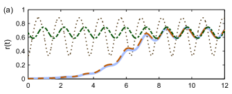
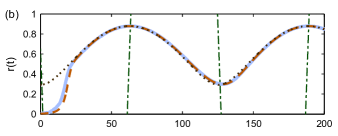
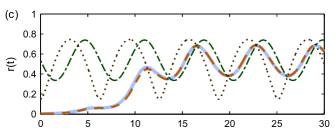
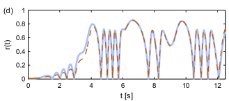
Model A is also solvable with an independent Lorentzian distribution of forcing strengths. The frequencies follow $\tilde{\omega}(t)=\omega+Ix(t)$ and the mean and half-width of $h(I)$ are $\hat{I}$ and $\gamma_{I}$ respectively. The integrals in Eq. (13) can again be closed in the lower or upper complex half-plane, and the requirements for $\alpha(\omega,I,t)$ are similar to those in the previous case. Hence, the $I$ integral for $x(t)>0$ is around the pole $I_{p1}=(\hat{I}+i\gamma_{I})$ and around $I_{p2}=(\hat{I}-i\gamma_{I})$ otherwise, while in the $\omega$ integral the encircling is around the pole $\omega_{p2}=\hat{\omega}-i\gamma$. Thus, the residues give

$$z^{\ast}=\alpha(\hat{\omega}-i\gamma,\hat{I}-i\gamma_{I},t),$$

which is applied in Eq. (11), so we finally obtain

$$\dot{r}=-r[\gamma+\gamma_{I}|x(t)|+\frac{K}{2}(r^{2}-1)],\ \dot{\psi}=\hat{\omega}+\hat{I}x(t).\ \$$ (15)

A similar analysis would be possible for any other polynomial Lorentzian-like distributions of $\omega$ and $I$.

The only other analytically solvable form of model A that we are aware of is with multimodal $\delta$-distributed external strengths. For simplicity we choose the bimodal function

$$h(I)=\frac{1}{2}[\delta(I-\hat{I}-\gamma_{I})+\delta(I-\hat{I}+\gamma_{I})].$$

The integral (13) now leads to

$$z^{\ast}=\frac{1}{2}[\alpha_{1}(\hat{\omega}-i\gamma,\hat{I}-\gamma_{I},t)+\alpha_{2}(\hat{\omega}-i\gamma,\hat{I}+\gamma_{I},t)],\ \ \ \ \$$ (16)

with dynamics consistently described by the evolutions of $\alpha_{1,2}$ obtained from Eq. (11),

$$\frac{\partial\alpha_{1,2}}{\partial t}=-\{i[\hat{\omega}+(\hat{I}\mp\gamma_{I})x(t)]-\gamma\}\alpha_{1,2}+$$

$$\ \ \ \ \ \ \ \ \ \ +\frac{K}{4}[\alpha_{1}+\alpha_{2}-\alpha_{1,2}^{2}(\alpha_{1}+\alpha_{2})^{\ast}].$$ (17)

This case of model A was also investigated in Choi , where Choi et al. carried out a bifurcation analysis near the limit $rK\ll 1$.

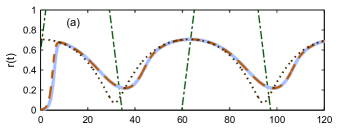
Following the restrictions on $x(t)$ in the problems analyzed in Fig. 1, we took

$$x(t)=\cos\Omega t\ \ \text{and}\ \ \epsilon<1$$

in the case of strength proportional to the frequency, while for model A with independent Lorentzianly-distributed strengths, the forcing is

$$x(t)=1+\cos\Omega t.$$

Finally, for bimodal $\delta$-distributed strengths, the absence of restrictions on the external field allows it to be the $x$ component of a Rössler oscillator Rossler . In all the problems shown, the NA TD dynamics is revealed and fully described by the reduced NA low-dimensional system. A Runge-Kutta 4 algorithm was used for numerical integration of Eqs. (1, 2) over $100000$ oscillators, with a time-step of $0.0025s$, while half-width and mean of the natural frequencies were $\gamma=1$ and $\hat{\omega}=0$, except where otherwise stated.

III.2 Time-dependent coupling strengths

We have also investigated the low-dimensional evolution of NA model B, Eq. (2). Since all the couplings in the original model are equal, there is no qualitative difference between the situations with identical forcing to each coupling, and coupling-dependent forcing. We chose the latter and proceed as for model A, yielding

$$\dot{r}=-r[\gamma+\frac{K}{2}[1+\epsilon x(t)](r^{2}-1)];\ \ \ \dot{\psi}=\hat{\omega}.\ \ \ \$$ (18)

The analysis for multimodal $\delta$-distributed strengths is also very similar to that for model A (1). E.g. for bimodal $h(I)$, Eq. (16) holds again with $\alpha_{1,2}$ evolving as

$$\frac{\partial\alpha_{1,2}}{\partial t}=-(i\hat{\omega}-\gamma)\alpha_{1,2}+\frac{1}{4}K[1+(\hat{I}\mp\gamma_{I})x(t)]$$ (19)

$$\ \ \ \ \ \ \ \ \ \ \times[\alpha_{1}+\alpha_{2}-\alpha_{1,2}^{2}(\alpha_{1}+\alpha_{2})^{\ast}].$$

Figure 2: (color online) Time-varying mean field for model B, Eq. (2), follows the external cosine (a) or the chaotic (b) forcing. Numerical simulation of Eq. (2) (light blue) coincides with the low-dimensional evolution (dashed red), Eq. (18) – (a) and Eq. (19) – (b). (a) Adiabatic (dotted brown), Eq. (26), and non-adiabatic evolution (dashed-dotted green), Eq. (25) for constant forcing with $K=3$, $\Omega=0.1$ and $\epsilon=0.33$. (b) Bimodal $\delta$-distributed strengths with $K=5$, $\gamma_{I}=1$ and $\hat{I}=0$.

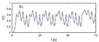
However, for a Lorentzian distribution $h(I)$, contour integration cannot be applied to Eq. (13). Namely, the integration contour should be such that if $\alpha(\omega,I,t)$ is analytic and $|\alpha|\leq 1$ everywhere inside the contour at $t=0$, this would also hold for all $t>0$. However, for this to happen, one of the requirements from Montbrio2011 is $|\alpha|\leq 0$, for $|\alpha|=1$. This should be taken in regard to the semicircular integration path $I=|I|e^{i\vartheta}$ with $|q|\rightarrow\infty$ and $\vartheta\in(0,\pi)$ or $\vartheta\in(-\pi,0)$ depending on the half-plane of the contour. Thus, substituting for $I$ into Eq. (12) and taking $|\alpha|=1$ , it yields

$$\frac{\partial|\alpha|}{\partial t}=|I|x(t)r\sin\vartheta\sin[\phi(\omega,I,t)-\psi(t)].$$ (20)

Here, $\phi$ is the phase of $\alpha$ that depends on $\omega$, $I$ and $t$, implying that the last sine can have either signs. Consequently, it cannot be proven that the condition $\frac{\partial{|\alpha|}}{\partial t}\leq 0$ holds for $\forall$ $t$ and $\omega$, on either of the half-planes. As a result, the integral in the Eq. (9) cannot be solved for $I$ using the residue theorem.

In contrast, the restrictions do not affect the NA parts of the other discussed variations of model B. To confirm this generality, $x(t)$ for the problem shown in Fig. 2 (b) is a chaotic signal from a Rössler oscillator. Similarly, the chosen amplitude of the cosine forcing in Fig. 2 (a) allows close-to-incoherent dynamics to be observed in some intervals, so that appear the limitations of the slow-fast approaches discussed in the following section.

A theorem in Ott2 states that Eqs. (11, 12) asymptotically capture all macroscopic behavior of the system as $t\rightarrow\infty$. Moreover the incoherent and partly synchronized states both belong to the manifold defined by Eqs. (11, 12) Ott1 , and initial incoherent state is set with uniformly distributed phases at time $t=0$. Thereafter, the ansatz (11, 12) and the evolutions (14-19) should continuously describe our system, as confirmed by Figs. 1 and 2.

IV Reduced dynamics

The plots in Figs. 1 (a)-(c) and 2 (a) show that the oscillations of the mean field follow the frequency of the external forcing, but this raises the questions of what is the amplitude of the oscillations and whether they can adiabatically follow the forcing. Similarly, an obvious feature of the same results is the low-frequency filtering of the external fields, i.e. the only difference between plots (a) and (b) of Fig. 1 is the frequency of the external forcing, while its influence is much more prominent in the latter. This is actually a well-known, but not much explored, characteristic of population models, and it is a direct consequence of their intrinsic transient dynamics Strogatz_sync .

In the following we adopt fast-slow reduction to simplify the evolution for simple periodic forcing. The reduction depends on the period of the external field $T=2\pi/\Omega$, relative to the system’s transition time, $\tau$, and has not been applied to similar systems. The exponential damping rate of the original system is defined by $\tau$ Ott1 and

$$\tau=1/|K/2-\gamma|.$$

For a system far from incoherence, $K=2\gamma+{\rm O}(2\gamma)$, $\tau\approx 1/{\rm O}(\gamma)$ holds, meaning that the transition time depends only on the width of the distribution of natural frequencies. Thereafter for this case, the system’s response is adiabatic for slow external fields, $\Omega\ll\gamma$, and non-adiabatic for fast, $\Omega\gg\gamma$. From now on, the dependence on $\gamma$ is removed by scaling the time and the couplings in the autonomous system, $t=t/\gamma$, $K=K/2\gamma$ and $\tau=1/|K-1|$ (the scaled variables keep the same letters).

For model A, Eq. (1), with $x(t)=\cos\Omega t$ and $h(I)=\delta(I-\epsilon)$, after the initial transition and in the absence of bifurcations, the amplitude of the mean field consists of a constant term $r_{0}$ and a TD term $\Delta r(t)$. For the non-adiabatic response, simulations, grey lines in Fig. 1(a), show that $\Delta r(t)\sim 1/\Omega$ and $r_{0}\gg\Delta r(t)$. Thereafter $r_{0}$ can be expressed as averaged over one period $T=2\pi/\Omega$ of the oscillations of $\Delta r(t)$. This way it follows $0=-r_{0}+K(r_{0}^{3}-r_{0})$ comment , or

$$r_{0}=\sqrt{1-1/K}.$$

Further, we apply $r(t)\approx r_{0}$ and $\frac{dr}{dt}=\frac{d\Delta r}{dt}$ to Eq. (14) and then integrate it. From there

$$\Delta r(t)=-r_{0}\frac{\epsilon}{\Omega}\sin\Omega t,$$

and the magnitude of the NA response is

$$\Delta_{\rm fast}=2\frac{\epsilon}{\Omega}\sqrt{1-\frac{1}{K}}.$$ (21)

Hence the long-term non-adiabatic evolution follows

$$r_{\rm fast}(t)=\sqrt{1-\frac{1}{K}}(1-\frac{\epsilon}{\Omega}\sin\Omega t).$$ (22)

The adiabatic behavior emerges through the introduction of a slow time-scale $t^{\prime}=\Omega t$, such that the system is constant on the fast time-scale $t$, and changes only in $t^{\prime}$. Hence the l.h.s. of Eq. (14) is zero, whence

$$r_{\rm slow}(t)=\sqrt{1-\frac{1+\epsilon\cos\Omega t}{K}},$$ (23)

while, for the magnitude of the NA part, we obtain

$$\Delta_{\rm slow}=\sqrt{1-\frac{1-\epsilon}{K}}-\sqrt{1-\frac{1+\epsilon}{K}}.$$ (24)

An analogous analysis can be performed for the appropriate form of model B, Eq. (2), leading to the low-dimensional evolution for fast cosine forcing given by

$$r_{\rm fast}(t)=\left(1+\frac{\epsilon}{\Omega}\sin\Omega t\right)\sqrt{1-\frac{1}{K}},$$ (25)

and for slow forcing

$$r_{\rm slow}(t)=\sqrt{1-\frac{1}{K(1+\epsilon\cos\Omega t)}}.$$ (26)

For the dynamics of model A with independent Lorentzian strengths and cosine forcing, $x(t)=1+\cos\Omega t$, the time is scaled by $(\gamma+\gamma_{I})$, and the dynamics follows

$$r_{\rm fast}(t)=\sqrt{1-\frac{1}{K}}[1-\frac{\gamma_{I}}{\Omega(\gamma+\gamma_{I})}\sin\Omega t]$$ (27)

for fast forcing, while for slow driving

$$r_{\rm slow}(t)=\sqrt{1-\frac{1}{K}-\frac{\gamma_{I}\cos\Omega t}{K(\gamma+\gamma_{I})}}.$$ (28)

The adiabatic responses can also be obtained from the self-consistency of Eqs. (7, 9) for stationary states of the mean field. Namely, assuming very slow dynamics of the external forcing, the system can be treated as quasistationary. This is similar to assuming stationarity on a fast time scale. Thus one obtains

$$r=\sqrt{1-2\gamma(t)/K(t)},$$

which corresponds to the results (23), (26).

Figure 3: (color online) Magnitude of the response, $\Delta(\epsilon,\Omega)$, of the NA model A to the cosine forcing, Eq. (1). External forcing strengths follow the distribution of frequencies, $K=4.25$ and $\Omega\in[10^{-2},10^{2}]$. (a) Results from Eq. (14) for $\epsilon\in[0.05,0.99]$. (b) Non-adiabatic (dotted black), Eq. (21) and adiabatic, Eq. (24), (dashed black) evolution for $\epsilon\in\{0.05,0.1055,0.2225,0.4693,0.99\}$, compared with the real dynamics (light blue), Eq. (14).

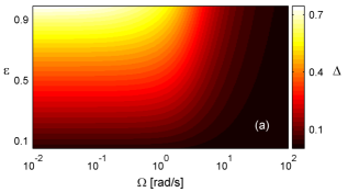
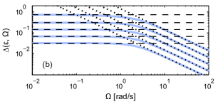
All the evolutions for reduced dynamics, Fig. 1(a)-(c) and 2(a), are in line with the above analysis, confirming the interplay between external and internal time scales of the NA system. The magnitudes of the slow/fast responses to cosine forcing are given in Fig. 3 for model A, Eq. (1), with forcing strengths following the frequencies’ distribution. They confirm the obtained dependance of $\Delta$ on the frequency and amplitude of the external field. The low-frequency filtering mentioned before is also obvious. The transient behavior for slow and fast forcing can be seen in Fig. 3(b), where $\Delta$ is shown for both the actual and the reduced dynamics. This plot perfectly matches the analytic limits for application of the reduction approaches. Similar plots can also be obtained for the other problems analyzed. However, for coupling close to critical, the system’s transition time increases and for $K\approx K_{c}$, $\tau\rightarrow\infty$. As a result, the slow dynamics fails, as shown in Fig. 2(a) at the minima of $r$ when it is close to $0$, unlike the case $K=K_{c}+{\rm O}(K_{c})$ given in Fig. 1(a)-(b) or Fig. 2(a) for $r$ far from 0.

V Discussion

With the analysis of the reduced dynamics, supplementing the full low-dimensional description, all aspects of the TD KM have been demonstrated. The former is shown only for simple periodic forcing, but this does not decrease the generality of the reduction, since any external field can be represented by its Fourier components. These methods are of great importance in modeling systems with multiple time-scales of oscillation and interaction, such as the human cardiovascular system Aneta1 , or inhibitory neurons in the cortex Wechselberger:09 .

In summary, we have characterised a new dynamics of interacting oscillators subject to continuous, deterministic perturbation. It consists of the dynamics of an external system superimposed on the original collective rhythm and was missing from earlier models Acebron_review , possibly leading to an incorrect interpretation of some real dynamical systems. We have derived the impact of the forcing and evaluated the effect of its dynamics, amplitude and distribution. Thus, we have proposed a generalization of the Kuramoto model that encompasses NA systems Rasmussen_book and is directly applicable to any thermodynamically open system. For example, the observed time-variations of brain dynamics can be easily explained as a consequence of TD frequencies or couplings of the single neurons, where the source of the external variation could be due to anaesthesia Jane1 , event-related Pfurtschelle:99 , or due to some influence from another part of the brain. In particular, the stable, time-varying mean field can now be reconstructed and, in this way, a large range of systems tackled by the Kuramoto model – spanning from a single cell up to the level of brain dynamics – can be described more realistically.

References

- (1) S. Strogatz. Sync: The Emerging Science of Spontaneous Order (Hyperion, New York, 2003).
- (2) Y. Kuramoto, Chemical Oscillations, Waves, and Turbulence (Springer-Verlag, Berlin, 1984).
- (3) J. A. Acebrón et al., Rev. Mod. Phys. 77, 137 (2005); S. H. Strogatz, Physica D 143, 1 (2000); A. Pikovsky, M. Rosenblum and J. Kurths, Synchronization – A Universal Concept in Nonlinear Sciences (CUP, Cambridge, 2001).
- (4) D. Rudrauf et al., Neuroimage 31, 209 (2006).
- (5) J. H. Sheeba, A. Stefanovska, and P. V. E. McClintock, Biophys. J. 95, 2722 (2008).
- (6) B. Musizza et al., J. Physiol. 580
- (7) G. Pfurtschelle and F. H. Lopes da Silva, Clin. Neurophysiol. 110, 1842 (1999).
- (8) Y. Shiogai, A. Stefanovska and P. V. E. McClintock, Phys. Reports 488, 51–110 (2010).
- (9) T. E. Lee and M. C. Cross, Phys. Rev. Lett. 106, 143001 (2011).
- (10) S. H. Strogatz and R. E. Mirollo, J. Statist. Phys. 63, 613 (1991).
- (11) S. Shinomoto and Y. Kuramoto, Prog. Theor. Phys. 75, 1105 (1986); H. Sakaguchi, Prog. Theor. Phys. 79, 39 (1988).
- (12) D. Cumin and C. Unsworth, Physica D 226, 181 (2007).
- (13) E. Montbrió, J. Kurths, and B. Blasius, Phys. Rev. E 70, 056125 (2004); J. H. Sheeba, V. K. Chandrasekar, A. Stefanovska, and P. V. E. McClintock, Phys. Rev. E 79, 046210 (2009);
- (14) L. L. Bonilla, J. C. Neu, and R. Spigler, J. Stat. Phys. 67, 313 (1992); J. A. Acebrón, L. L. Bonilla, S. De Leo and R. Spigler, Phys. Rev. E 57, 5287 (1998).
- (15) D. Taylor, E. Ott, J. G. Restrepo, Phys. Rev. E 81, 046214 (2010).
- (16) J. A. Acebrón and R. Spigler, Phys. Rev. Lett. 81, 2229 (1998).
- (17) J. Rougemont and F. Naef, Phys. Rev. E 73, 011104 (2006).
- (18) P. So, A. Bernard B. C. Cotton, and E. Barreto , Chaos 18, 037114 (2008); S. P. Kuznetsov, A. Pikovsky, and M. Rosenblum, Chaos 20, 043134 (2010).
- (19) S. H. Lee, S. Lee, S.-W. Son, and P. Holme, Phys. Rev. E 85, 027202 (2012).
- (20) J. H. Sheeba, V. K. Chandrasekar, and M. Lakshmanan, Phys. Rev. E 84, 036210 (2011).
- (21) R. Mirollo and S. H. Strogatz, J. Nonlinear Sci. 17, 309 (2007).
- (22) E. Ott and T. M. Antonsen, Chaos 18, 037113 (2008).
- (23) M. Y. Choi, Y. W. Kim, and D. C. Hong, Phys. Rev. E 49, 3825 (1994).
- (24) O. E. Rössler, Synergetics (a workshop), ed. H. Haken (Springer, Berlin, 1977) p. 184.
- (25) E. Montbrió and D. Pazó, Phys. Rev. Lett. 106, 254101 (2011).
- (26) E. Ott and T. M. Antonsen, Chaos 19, 023117 (2009).
- (27) This is obtained from averaging both sides of Eq. (14) for one period. The term in the integral vanishes only if , which is self-consistently proved as the obtained form of for non-adiabatic response, Eq. (22), follows this assumption.
- (28) A. Stefanovska and M. Brai, Contemp. Phys. 40, 31 (1999).
- (29) B. Ermentrout and M. Wechselberger. SIAM J. Appl. Dyn. Syst. 8 253 (2009).
- (30) M. Rasmussen, Attractivity and Bifurcation for Nonautonomous Dynamical Systems, (Lecture Notes in Mathematics 1907) (Springer, 2007).