Bayesian analysis of the astrobiological implications of life’s early emergence on Earth

Abstract

Life arose on Earth sometime in the first few hundred million years after the young planet had cooled to the point that it could support water-based organisms on its surface. The early emergence of life on Earth has been taken as evidence that the probability of abiogenesis is high, if starting from young-Earth-like conditions. We revisit this argument quantitatively in a Bayesian statistical framework. By constructing a simple model of the probability of abiogenesis, we calculate a Bayesian estimate of its posterior probability, given the data that life emerged fairly early in Earth’s history and that, billions of years later, curious creatures noted this fact and considered its implications. We find that, given only this very limited empirical information, the choice of Bayesian prior for the abiogenesis probability parameter has a dominant influence on the computed posterior probability. Although terrestrial life’s early emergence provides evidence that life might be common in the Universe if early-Earth-like conditions are, the evidence is inconclusive and indeed is consistent with an arbitrarily low intrinsic probability of abiogenesis for plausible uninformative priors. Finding a single case of life arising independently of our lineage (on Earth, elsewhere in the Solar System, or on an extrasolar planet) would provide much stronger evidence that abiogenesis is not extremely rare in the Universe.

Gyr, gigayear ($10^{9}$ years); PDF, probability density function; CDF, cumulative distribution function

1 Introduction

Astrobiology is fundamentally concerned with whether extraterrestrial life exists and, if so, how abundant it is in the Universe. The most direct and promising approach to answering these questions is surely empirical, the search for life on other bodies in the Solar System [1, 2] and beyond in other planetary systems [3, 4]. Nevertheless, a theoretical approach is possible in principle and could provide a useful complement to the more direct lines of investigation.

In particular, if we knew the probability per unit time and per unit volume of abiogenesis in a pre-biotic environment as a function of its physical and chemical conditions and if we could determine or estimate the prevalence of such environments in the Universe, we could make a statistical estimate of the abundance of extraterrestrial life. This relatively straightforward approach is, of course, thwarted by our great ignorance regarding both inputs to the argument at present.

There does, however, appear to be one possible way of finessing our lack of detailed knowledge concerning both the process of abiogenesis and the occurrence of suitable pre-biotic environments (whatever they might be) in the Universe. Namely, we can try to use our knowledge that life arose at least once in an environment (whatever it was) on the early Earth to try to infer something about the probability per unit time of abiogenesis on an Earth-like planet without the need (or ability) to say how Earth-like it need be or in what ways. We will hereinafter refer to this probability per unit time, which can also be considered a rate, as $\lambda$ or simply the “probability of abiogenesis.”

Any inferences about the probability of life arising (given the conditions present on the early Earth) must be informed by how long it took for the first living creatures to evolve. By definition, improbable events generally happen infrequently. It follows that the duration between events provides a metric (however imperfect) of the probability or rate of the events. The time-span between when Earth achieved pre-biotic conditions suitable for abiogenesis plus generally habitable climatic conditions [5, 6, 7] and when life first arose, therefore, seems to serve as a basis for estimating $\lambda$. Revisiting and quantifying this analysis is the subject of this paper.

We note several previous quantitative attempts to address this issue in the literature, of which one [8] found, as we do, that early abiogenesis is consistent with life being rare, and the other [9] found that Earth’s early abiogenesis points strongly to life being common on Earth-like planets (we compare our approach to the problem to that of [9] below, including our significantly different results). Furthermore, an argument of this general sort has been widely used in a qualitative and even intuitive way to conclude that $\lambda$ is unlikely to be extremely small because it would then be surprising for abiogenesis to have occurred as quickly as it did on Earth [12, 13, 14, 15, 16, 17, 18]. Indeed, the early emergence of life on Earth is often taken as significant supporting evidence for “optimism” about the existence of extra-terrestrial life (i.e., for the view that it is fairly common) [19, 20, 9]. The major motivation of this paper is to determine the quantitative validity of this inference. We emphasize that our goal is not to derive an optimum estimate of $\lambda$ based on all of the many lines of available evidence, but simply to evaluate the implication of life’s early emergence on Earth for the value of $\lambda$.

2 A Bayesian Formulation of the Calculation

Bayes’s theorem [21] can be written as ${\rm P}[\mathcal{M}|\mathcal{D}]=\left({\rm P}[\mathcal{D}|\mathcal{M}]\times{\rm P}_{\rm prior}[\mathcal{M}]\right)/{\rm P}[\mathcal{D}]$. Here, we take $\mathcal{M}$ to be a model and $\mathcal{D}$ to be data. In order to use this equation to evaluate the posterior probability of abiogenesis, we must specify appropriate $\mathcal{M}$ and $\mathcal{D}$.

2.1 A Poisson or Uniform Rate Model

In considering the development of life on a planet, we suggest that a reasonable, if simplistic, model is that it is a Poisson process during a period of time from $t_{\rm min}$ until $t_{\rm max}$. In this model, the conditions on a young planet preclude the development of life for a time period of $t_{\rm min}$ after its formation. Furthermore, if the planet remains lifeless until $t_{\rm max}$ has elapsed, it will remain lifeless thereafter as well because conditions no longer permit life to arise. For a planet around a solar-type star, $t_{\rm max}$ is almost certainly  $\sim$$<$ 10 Gyr (10 billion years, the main sequence lifetime of the Sun) and could easily be a substantially shorter period of time if there is something about the conditions on a young planet that are necessary for abiogenesis. Between these limiting times, we posit that there is a certain probability per unit time ($\lambda$) of life developing. For $t_{\rm min}<t<t_{\rm max}$, then, the probability of life arising $n$ times in time $t$ is

$${\rm P}[\lambda,n,t]={\rm P}_{\rm Poisson}[\lambda,n,t]=e^{-\lambda(t-t_{\rm min})}\frac{\{\lambda(t-t_{\rm min})\}^{n}}{n!}\,,$$ (1)

where $t$ is the time since the formation of the planet.

This formulation could well be questioned on a number of grounds. Perhaps most fundamentally, it treats abiogenesis as though it were a single instantaneous event and implicitly assumes that it can occur in only a single way (i.e., by only a single process or mechanism) and only in one type of physical environment. It is, of course, far more plausible that abiogenesis is actually the result of a complex chain of events that take place over some substantial period of time and perhaps via different pathways and in different environments. However, knowledge of the actual origin of life on Earth, to say nothing of other possible ways in which it might originate, is so limited that a more complex model is not yet justified. In essence, the simple Poisson event model used in this paper attempts to “integrate out” all such details and treat abiogenesis as a “black box” process: certain chemical and physical conditions as input produce a certain probability of life emerging as an output. Another issue is that $\lambda$, the probability per unit time, could itself be a function of time. In fact, the claim that life could not have arisen outside the window $(t_{\rm min},t_{\rm max})$ is tantamount to saying that $\lambda=0$ for $t\leq t_{\rm min}$ and for $t\geq t_{\rm max}$. Instead of switching from 0 to a fixed value instantaneously, $\lambda$ could exhibit a complicated variation with time. If so, however, ${\rm P}[\lambda,n,t]$ is not represented by the Poisson distribution and eq. (1) is not valid. Unless a particular (non top-hat-function) time-variation of $\lambda$ is suggested on theoretical grounds, it seems unwise to add such unconstrained complexity.

A further criticism is that $\lambda$ could be a function of $n$: it could be that life arising once (or more) changes the probability per unit time of life arising again. Since we are primarily interested in the probability of life arising at all – i.e., the probability of $n\neq 0$ – we can define $\lambda$ simply to be the value appropriate for a prebiotic planet (whatever that value may be) and remain agnostic as to whether it differs for $n\geq 1$. Thus, within the adopted model, the probability of life arising is one minus the probability of it not arising:

$${\rm P}_{\rm life}=1-{\rm P}_{\rm Poisson}[\lambda,0,t]=1-e^{-\lambda(t-t_{\rm min})}\,.$$ (2)

2.2 A Minimum Evolutionary Time Constraint

Naively, the single datum informing our calculation of the posterior of $\lambda$ appears to be simply that life arose on Earth at least once, approximately 3.8 billion years ago (give or take a few hundred million years). There is additional significant context for this datum, however. Recall that the standard claim is that, since life arose early on the only habitable planet that we have examined for inhabitants, the probability of abiogenesis is probably high (in our language, $\lambda$ is probably large). This standard argument neglects a potentially important selection effect, namely: On Earth, it took nearly 4 Gyr for evolution to lead to organisms capable of pondering the probability of life elsewhere in the Universe. If this is a necessary duration, then it would be impossible for us to find ourselves on, for example, a ($\sim$4.5-Gyr old) planet on which life first arose only after the passage of 3.5 billion years [22]. On such planets there would not yet have been enough time for creatures capable of such contemplations to evolve. In other words, if evolution requires 3.5 Gyr for life to evolve from the simplest forms to intelligent, questioning beings, then we had to find ourselves on a planet where life arose relatively early, regardless of the value of $\lambda$.

In order to introduce this constraint into the calculation we define $\delta t_{\rm evolve}$ as the minimum amount of time required after the emergence of life for cosmologically curious creatures to evolve, $t_{\rm emerge}$ as the age of the Earth from when the earliest extant evidence of life remains (though life might have actually emerged earlier), and $t_{0}$ as the current age of the Earth. The data, then, are that life arose on Earth at least once, approximately 3.8 billion years ago, and that this emergence was early enough that human beings had the opportunity subsequently to evolve and to wonder about their origins and the possibility of life elsewhere in the Universe. In equation form, $t_{\rm emerge}<t_{0}-\delta t_{\rm evolve}$.

Models of $t_{0}=4.5$ Gyr-Old Planets
Model Hypothetical Conserv.₁ Conserv.₂ Optimistic   $t_{\rm min}$ 0.5 0.5 0.5 0.5 $t_{\rm emerge}$ 0.51 1.3 1.3 0.7 $t_{\rm max}$ 10 1.4 10 10 $\delta t_{\rm evolve}$ 1 2 3.1 1 $t_{\rm required}$ 3.5 1.4 1.4 3.5 $\Delta t_{1}$ 0.01 0.80 0.80 0.20 $\Delta t_{2}$ 3.00 0.90 0.90 3.00 $\mathcal{R}$ 300 1.1 1.1 15

All times are in Gyr. Two “Conservative” (Conserv.) models are shown, to indicate that $t_{\rm required}$ may be limited either by a small value of $t_{\rm max}$ (“Conserv.₁”), or by a large value of $\delta t_{\rm evolve}$ (“Conserv.₂”).

2.3 The Likelihood Term

We now seek to evaluate the ${\rm P}[\mathcal{D}|\mathcal{M}]$ term in Bayes’s theorem. Let $t_{\rm required}\equiv\min[t_{0}-\delta t_{\rm evolve},t_{\rm max}]$. Our existence on Earth requires that life appeared within $t_{\rm required}$. In other words, $t_{\rm required}$ is the maximum age that the Earth could have had at the origin of life in order for humanity to have a chance of showing up by the present. We define $\mathcal{S_{E}}$ to be the set of all Earth-like worlds of age approximately $t_{0}$ in a large, unbiased volume and $L[t]$ to be the subset of $\mathcal{S_{E}}$ on which life has emerged within a time $t$. $L[t_{\rm required}]$ is the set of planets on which life emerged early enough that creatures curious about abiogenesis could have evolved before the present ($t_{0}$), and, presuming $t_{\rm emerge}<t_{\rm required}$ (which we know was the case for Earth), $L[t_{\rm emerge}]$ is the subset of $L[t_{\rm required}]$ on which life emerged as quickly as it did on Earth. Correspondingly, $N_{\mathcal{S_{E}}}$, $N_{t_{\rm r}}$, and $N_{t_{\rm e}}$ are the respective numbers of planets in sets $\mathcal{S_{E}}$, $L[t_{\rm required}]$, and $L[t_{\rm emerge}]$. The fractions $\varphi_{t_{\rm r}}\equiv N_{t_{\rm r}}/N_{\mathcal{S_{E}}}$ and $\varphi_{t_{\rm e}}\equiv N_{t_{\rm e}}/N_{\mathcal{S_{E}}}$ are, respectively, the fraction of Earth-like planets on which life arose within $t_{\rm required}$ and the fraction on which life emerged within $t_{\rm emerge}$. The ratio $r\equiv\varphi_{t_{\rm e}}/\varphi_{t_{\rm r}}=N_{t_{\rm e}}/N_{t_{\rm r}}$ is the fraction of $L_{t_{\rm r}}$ on which life arose as soon as it did on Earth. Given that we had to find ourselves on such a planet in the set $L_{t_{\rm r}}$ in order to write and read about this topic, the ratio $r$ characterizes the probability of the data given the model if the probability of intelligent observers arising is independent of the time of abiogenesis (so long as abiogenesis occurs before $t_{\rm required}$). (This last assumption might seem strange or unwarranted, but the effect of relaxing this assumption is to make it more likely that we would find ourselves on a planet with early abiogenesis and therefore to reduce our limited ability to infer anything about $\lambda$ from our observations.) Since $\varphi_{t_{\rm e}}=1-{\rm P}_{\rm Poisson}[\lambda,0,t_{\rm emerge}]$ and $\varphi_{t_{\rm r}}=1-{\rm P}_{\rm Poisson}[\lambda,0,t_{\rm required}]$, we may write that

$${\rm P}[\mathcal{D}|\mathcal{M}]=\frac{1-\exp[-\lambda(t_{\rm emerge}-t_{\rm min})]}{1-\exp[-\lambda(t_{\rm required}-t_{\rm min})]}$$ (3)

if $t_{\rm min}<t_{\rm emerge}<t_{\rm required}$ (and ${\rm P}[\mathcal{D}|\mathcal{M}]=0$ otherwise). This is called the “likelihood function,” and represents the probability of the observation(s), given a particular model. It is via this function that the data “condition” our prior beliefs about $\lambda$ in standard Bayesian terminology.

2.4 Limiting Behavior of the Likelihood

It is instructive to consider the behavior of equation (3) in some interesting limits. For $\lambda(t_{\rm required}-t_{\rm min})\ll 1$, the numerator and denominator of equation (3) each go approximately as the argument of the exponential function; therefore, in this limit, the likelihood function is approximately constant:

$${\rm P}[\mathcal{D}|\mathcal{M}]\approx\frac{t_{\rm emerge}-t_{\rm min}}{t_{\rm required}-t_{\rm min}}\,.$$ (4)

This result is intuitively easy to understand as follows: If $\lambda$ is sufficiently small, it is overwhelmingly likely that abiogenesis occurred only once in the history of the Earth, and by the assumptions of our model, the one event is equally likely to occur at any time during the interval between $t_{\rm min}$ and $t_{\rm required}$. The chance that this will occur by $t_{\rm emerge}$ is then just the fraction of that total interval that has passed by $t_{\rm emerge}$ – the result given in equation (4).

In the other limit, when $\lambda(t_{\rm emerge}-t_{\rm min})\gg 1$, the numerator and denominator of equation (3) are both approximately 1. In this case, the likelihood function is also approximately constant (and equal to unity). This result is even more intuitively obvious since a very large value of $\lambda$ implies that abiogenesis events occur at a high rate (given suitable conditions) and are thus likely to have occurred very early in the interval between $t_{\rm min}$ and $t_{\rm required}$.

These two limiting cases, then, already reveal a key conclusion of our analysis: the posterior distribution of $\lambda$ for both very large and very small values will have the shape of the prior, just scaled by different constants. Only when $\lambda$ is neither very large nor very small – or, more precisely, when $\lambda(t_{\rm emerge}-t_{\rm min})\approx 1$ – do the data and the prior both inform the posterior probability at a roughly equal level.

2.5 The Bayes Factor

In this context, note that the probability in equation (3) depends crucially on two time differences, $\Delta t_{1}\equiv t_{\rm emerge}-t_{\rm min}$ and $\Delta t_{2}\equiv t_{\rm required}-t_{\rm min}$, and that the ratio of the likelihood function at large $\lambda$ to its value at small $\lambda$ goes roughly as

$$\mathcal{R}\equiv\frac{{\rm P}[\rm data|large~{}\lambda]}{{\rm P}[\rm data|small~{}\lambda]}\approx\frac{\Delta t_{2}}{\Delta t_{1}}\,.$$ (5)

$\mathcal{R}$ is called the Bayes factor or Bayes ratio and is sometimes employed for model selection purposes. In one conventional interpretation [23], $\mathcal{R}\leq 10$ implies no strong reason in the data alone to prefer the model in the numerator over the one in the denominator. For the problem at hand, this means that the datum does not justify preference for a large value of $\lambda$ over an arbitrarily small one unless equation (5) gives a result larger than roughly ten.

Since the likelihood function contains all of the information in the data and since the Bayes factor has the limiting behavior given in equation 5, our analysis in principle need not consider priors. If a small value of $\lambda$ is to be decisively ruled out by the data, the value of $\mathcal{R}$ must be much larger than unity. It is not for plausible choices of the parameters (see Table 1), and thus arbitrarily small values of $\lambda$ can only be excluded by some adopted prior on its values. Still, for illustrative purposes, we now proceed to demonstrate the influence of various possible $\lambda$ priors on the $\lambda$ posterior.

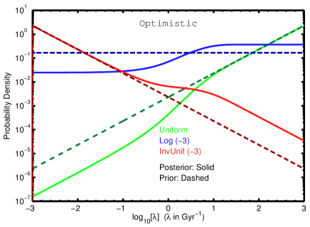
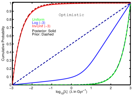
Figure 1: PDF and CDF of $\lambda$ for uniform, logarithmic, and inverse-uniform priors, for model Optimistic, with $\lambda_{\rm min}=10^{-3}\rm~{}Gyr^{-1}$ and $\lambda_{\rm max}=10^{3}\rm~{}Gyr^{-1}$. Top: The dashed and solid curves represent, respectively, the prior and posterior probability distribution functions (PDFs) of $\lambda$ under three different assumptions about the nature of the prior. The green curves are for a prior that is uniform on the range $0{\rm~{}Gyr^{-1}}\leq\lambda\leq\lambda_{\rm max}$ (“Uniform”); the blue are for a prior that is uniform in the log of $\lambda$ on the range $-3\leq\log\lambda\leq 3$ (“Log (-3)”); and the red are for a prior that is uniform in $\lambda^{-1}$ on the interval $10^{-3}{\rm~{}Gyr}\leq\lambda^{-1}\leq 10^{3}{\rm~{}Gyr}$ (“InvUnif (-3)”). Bottom: The curves represent the cumulative distribution functions (CDFs) of $\lambda$. The ordinate on each curve represents the integrated probability from 0 to the abscissa (color and line-style schemes are the same as in the top panel). For a uniform prior, the posterior CDF traces the prior almost exactly. In this case, the posterior judgment that $\lambda$ is probably large simply reflects the prior judgment of the distribution of $\lambda$. For the prior that is uniform in $\lambda^{-1}$ (InvUnif), the posterior judgment is quite opposite – namely, that $\lambda$ is probably quite small – but this judgment is also foretold by the prior, which is traced nearly exactly by the posterior. For the logarithmic prior, the datum (that life on Earth arose within a certain time window) does influence the posterior assessment of $\lambda$, shifting it in the direction of making greater values of $\lambda$ more probable. Nevertheless, the posterior probability is $\sim$12% that $\lambda<1\rm~{}Gyr^{-1}$. Lower $\lambda_{\rm min}$ and/or lower $\lambda_{\rm max}$ would further increase the posterior probability of very low $\lambda$, for any of the priors.

2.6 The Prior Term

To compute the desired posterior probability, what remains to be specified is ${\rm P}_{\rm prior}[\mathcal{M}]$, the prior joint probability density function (PDF) of $\lambda$, $t_{\rm min}$, $t_{\rm max}$, and $\delta t_{\rm evolve}$. One approach to choosing appropriate priors for $t_{\rm min}$, $t_{\rm max}$, and $\delta t_{\rm evolve}$, would be to try to distill geophysical and paleobiological evidence along with theories for the evolution of intelligence and the origin of life into quantitative distribution functions that accurately represent prior information and beliefs about these parameters. Then, in order to ultimately calculate a posterior distribution of $\lambda$, one would marginalize over these “nuisance parameters.” However, since our goal is to evaluate the influence of life’s early emergence on our posterior judgment of $\lambda$ (and not of the other parameters), we instead adopt a different approach. Rather than calculating a posterior over this 4-dimensional parameter space, we investigate the way these three time parameters affect our inferences regarding $\lambda$ by simply taking their priors to be delta functions at several theoretically interesting values: a purely hypothetical situation in which life arose extremely quickly, a most conservative situation, and an in between case that is also optimistic but for which there does exist some evidence (see Table 1).

For the values in Table 1, the likelihood ratio $\mathcal{R}$ varies from $\sim$1.1 to 300, with the parameters of the “optimistic” model giving a borderline significance value of $\mathcal{R}=15$. Thus, only the hypothetical case gives a decisive preference for large $\lambda$ by the Bayes factor metric, and we emphasize that there is no direct evidence that abiogenesis on Earth occurred that early, only 10 million years after conditions first permitted it!

We also lack a first-principles theory or other solid prior information for $\lambda$. We therefore take three different functional forms for the prior – uniform in $\lambda$, uniform in $\lambda^{-1}$ (equivalent to saying that the mean time until life appears is uniformly distributed), and uniform in $\log_{10}\lambda$. For the uniform in $\lambda$ prior, we take our prior confidence in $\lambda$ to be uniformly distributed on the interval 0 to $\lambda_{\rm max}=1000$ $\rm~{}Gyr^{-1}$ (and to be 0 otherwise). For the uniform in $\lambda^{-1}$ and the uniform in $\log_{10}[\lambda]$ priors, we take the prior density functions for $\lambda^{-1}$ and $\log_{10}[\lambda]$, respectively, to be uniform on $\lambda_{\rm min}\leq\lambda\leq\lambda_{\rm max}$ (and 0 otherwise). For illustrative purposes, we take three values of $\lambda_{\rm min}$: $10^{-22}\rm~{}Gyr^{-1}$, $10^{-11}\rm~{}Gyr^{-1}$, and $10^{-3}\rm~{}Gyr^{-1}$, corresponding roughly to life occuring once in the observable Universe, once in our galaxy, and once per 200 stars (assuming one Earth-like planet per star).

In standard Bayesian terminology, both the uniform in $\lambda$ and the uniform in $\lambda^{-1}$ priors are said to be highly “informative.” This means that they strongly favor large and small, respectively, values of $\lambda$ in advance, i.e., on some basis other than the empirical evidence represented by the likelihood term. For example, the uniform in $\lambda$ prior asserts that we know on some other basis (other than the early emergence of life on Earth) that it is a hundred times less likely that $\lambda$ is less than $10^{-3}\rm~{}Gyr^{-1}$ than that it is less than $0.1\rm~{}Gyr^{-1}$. The uniform in $\lambda^{-1}$ prior has the equivalent sort of preference for small $\lambda$ values. By contrast, the logarithmic prior is relatively “uninformative” in standard Bayesian terminology and is equivalent to asserting that we have no prior information that informs us of even the order-of-magnitude of $\lambda$.

In our opinion, the logarithmic prior is the most appropriate one given our current lack of knowledge of the process(es) of abiogenesis, as it represents scale-invariant ignorance of the value of $\lambda$. It is, nevertheless, instructive to carry all three priors through the calculation of the posterior distribution of $\lambda$, because they vividly illuminate the extent to which the result depends on the data vs the assumed prior.

2.7 Comparison with Previous Analysis

Using a binomial probability analysis, Lineweaver & Davis [9] attempted to quantify $q$, the probability that life would arise within the first billion years on an Earth-like planet. Although the binomial distribution typically applies to discrete situations (in contrast to the continuous passage of time, during which life might arise), there is a simple correspondence between their analysis and the Poisson model described above. The probability that life would arise at least once within a billion years (what [9] call $q$) is a simple transformation of $\lambda$, obtained from equation (2), with $\Delta t_{1}=1$ Gyr:

$$q=1-e^{-(\lambda)(1\rm~{}Gyr)}\qquad\mbox{or}\qquad\lambda=\ln[1-q]/(1\rm~{}Gyr)\,.$$ (6)

In the limit of $\lambda(1{\rm~{}Gyr})\ll 1$, equation (6) implies that $q$ is equal to $\lambda(1{\rm~{}Gyr})$. Though not cast in Bayesian terms, the analysis in [9] draws a Bayesian conclusion and therefore is based on an implicit prior that is uniform in $q$. As a result, it is equivalent to our uniform-$\lambda$ prior for small values of $\lambda$ (or $q$), and it is this implicit prior, not the early emergence of life on Earth, that dominates their conclusions.

3 The Posterior Probability of Abiogenesis

We compute the normalized product of the probability of the data given $\lambda$ (equation 3) with each of the three priors (uniform, logarithmic, and inverse uniform). This gives us the Bayesian posterior PDF of $\lambda$, which we also derive for each model in Table 1. Then, by integrating each PDF from $-\infty$ to $\lambda$, we obtain the corresponding cumulative distribution function (CDF).

Figure 1 displays the results by plotting the prior and posterior probability of $\lambda$. The top panel presents the PDF, and the bottom panel the CDF, for uniform, logarithmic, and inverse-uniform priors, for model Optimistic, which sets $\Delta t_{1}$ (the maximum time it might have taken life to emerge once Earth became habitable) to 0.2 Gyr, and $\Delta t_{2}$ (the time life had available to emerge in order that intelligent creatures would have a chance to evolve) to 3.0 Gyr. The dashed and solid curves represent, respectively, prior and posterior probability functions. In this figure, the priors on $\lambda$ have $\lambda_{\rm min}=10^{-3}\rm~{}Gyr^{-1}$ and $\lambda_{\rm max}=10^{3}\rm~{}Gyr^{-1}$. The green, blue, and red curves are calculated for uniform, logarithmic, and inverse-uniform priors, respectively. The results of the corresponding calculations for the other models and bounds on the assumed priors are presented in the Supporting Information, but the cases shown in Fig. 1 suffice to demonstrate all of the important qualitative behaviors of the posterior.

In the plot of differential probability (PDF; top panel), it appears that the inferred posterior probabilities of different values of $\lambda$ are conditioned similarly by the data (leading to a jump in the posterior PDF of roughly an order of magnitude in the vicinity of $\lambda\sim 0.5$ Gyr^-1). The plot of cumulative probability, however, immediately shows that the uniform and the inverse priors produce posterior CDFs that are completely insensitive to the data. Namely, small values of $\lambda$ are strongly excluded in the uniform in $\lambda$ prior case and large values are equally strongly excluded by the uniform in $\lambda^{-1}$ prior, but these strong conclusions are not a consequence of the data, only of the assumed prior. This point is particularly salient, given that a Bayesian interpretation of [9] indicates an implicit uniform prior. In other words, their conclusion that $q$ cannot be too small and thus that life should not be too rare in the Universe is not a consequence of the evidence of the early emergence of life on the Earth but almost only of their particular parameterization of the problem.

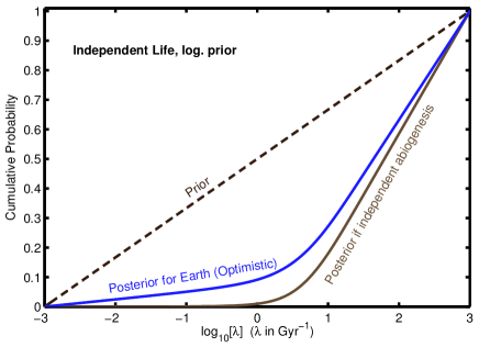
Figure 2: CDF of $\lambda$ for abiogenesis with independent lineage, for logarithmic prior. $\lambda_{\rm min}=10^{-3}\rm~{}Gyr^{-1}$, $\lambda_{\rm max}=10^{3}\rm~{}Gyr^{-1}$. A discovery that life arose independently on Mars and Earth or on an exoplanet and Earth – or that it arose a second, independent, time on Earth – would significantly reduce the posterior probability of low $\lambda$.

For the Optimistic parameters, the posterior CDF computed with the uninformative logarithmic prior does reflect the influence of the data, making greater values of $\lambda$ more probable in accordance with one’s intuitive expectations. However, with this relatively uninformative prior, there is a significant probability that $\lambda$ is very small (12% chance that $\lambda<1\rm~{}Gyr^{-1}$). Moreover, if we adopted smaller $\lambda_{\rm min}$, smaller $\lambda_{\rm max}$, and/or a larger $\Delta t_{1}/\Delta t_{2}$ ratio, the posterior probability of an arbitrarily low $\lambda$ value can be made acceptably high (see Fig. 3 and the Supporting Information).

3.1 Independent Abiogenesis

We have no strong evidence that life ever arose on Mars (although no strong evidence to the contrary either). Recent observations have tenatively suggested the presence of methane at the level of $\sim$20 parts per billion (ppb) [26], which could potentially be indicative of biological activity. The case is not entirely clear, however, as alternative analysis of the same data suggests that an upper limit to the methane abundance is in the vicinity of $\sim$3 ppb [27]. If, in the future, researchers find compelling evidence that Mars or an exoplanet hosts life that arose independently of life on Earth (or that life arose on Earth a second, independent time [28, 29]), how would this affect the posterior probability density of $\lambda$ (assuming that the same $\lambda$ holds for both instances of abiogenesis)?

If Mars, for instance, and Earth share a single $\lambda$ and life arose arise on Mars, then the likelihood of Mars’ $\lambda$ is the joint probability of our data on Earth and of life arising on Mars. Assuming no panspermia in either direction, these events are independent:

$${\rm P}[\mathcal{D}|\mathcal{M}] = \left(1-\exp[-\lambda(t_{\rm emerge}^{\rm Mars}-t_{\rm min}^{\rm Mars})]\right)$$ (7)

$$\times\frac{1-\exp[-\lambda(t_{\rm emerge}^{\rm Earth}-t_{\rm min}^{\rm Earth})]}{1-\exp[-\lambda(t_{\rm required}^{\rm Earth}-t_{\rm min}^{\rm Earth})]}\,.$$

For Mars, we take $t_{\rm max}^{\rm Mars}=t_{\rm emerge}^{\rm Mars}=1$ Gyr and $t_{\rm min}^{\rm Mars}=0.5$ Gyr. The posterior cumulative probability distribution of $\lambda$, given a logarithmic prior between 0.001 Gyr^-1 and 1000 Gyr^-1, is as represented in Fig. 2 for the case of finding a second, independent sample of life and, for comparison, the Optimistic case for Earth. Should future researchers find that life arose independently on Mars (or elsewhere), this would dramatically reduce the posterior probability of very low $\lambda$ relative to our current inferences.

3.2 Arbitrarily Low Posterior Probability of $\lambda$

We do not actually know what the appropriate lower (or upper) bounds on $\lambda$ are. Figure 3 portrays the influence of changing $\lambda_{\rm min}$ on the median posterior estimate of $\lambda$, and on 1-$\sigma$ and 2-$\sigma$ confidence lower bounds on posterior estimates of $\lambda$. Although the median estimate is relatvely insensitive to $\lambda_{\rm min}$, a 2-$\sigma$ lower bound on $\lambda$ becomes arbitrarily low as $\lambda_{\rm min}$ decreases.

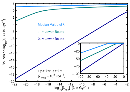
Figure 3: Lower bound on $\lambda$ for logarithmic prior, Hypothetical model. The three curves depict median (50%), 1-$\sigma$ (68.3%), and 2-$\sigma$ (95.4%) lower bounds on $\lambda$, as a function of $\lambda_{\rm min}$.

4 Conclusions

Within a few hundred million years, and perhaps far more quickly, of the time that Earth became a hospitable location for life, it transitioned from being merely habitable to being inhabited. Recent rapid progress in exoplanet science suggests that habitable worlds might be extremely common in our galaxy [30, 31, 32, 33], which invites the question of how often life arises, given habitable conditions. Although this question ultimately must be answered empirically, via searches for biomarkers [34] or for signs of extraterrestrial technology [35], the early emergence of life on Earth gives us some information about the probability that abiogenesis will result from early-Earth-like conditions.

A Bayesian approach to estimating the probability of abiogenesis clarifies the relative influence of data and of our prior beliefs. Although a “best guess” of the probability of abiogenesis suggests that life should be common in the Galaxy if early-Earth-like conditions are, still, the data are consistent (under plausible priors) with life being extremely rare, as shown in Figure 3. Thus, a Bayesian enthusiast of extraterrestrial life should be significantly encouraged by the rapid appearance of life on the early Earth but cannot be highly confident on that basis.

Our conclusion that the early emergence of life on Earth is consistent with life being very rare in the Universe for plausible priors is robust against two of the more fundamental simplifications in our formal analysis. First, we have assumed that there is a single value of $\lambda$ that applies to all Earth-like planets (without specifying exactly what we mean by “Earth-like”). If $\lambda$ actually varies from planet to planet, as seems far more plausible, anthropic-like considerations imply planets with particularly large $\lambda$ values will have a greater chance of producing (intelligent) life and of life appearing relatively rapidly, i.e., of the circumstances in which we find ourselves. Thus, the information we derive about $\lambda$ from the existence and early appearance of life on Earth will tend to be biased towards large values and may not be representative of the value of $\lambda$ for, say, an “average” terrestrial planet orbiting within the habitable zone of a main sequence star. Second, our formulation of the problem analyzed in this paper implicitly assumes that there is no increase in the probability of intelligent life appearing once $\delta t_{\rm evolve}$ has elapsed following the abiogenesis event on a planet. A more reasonable model in which this probability continues to increase as additional time passes would have the same qualitative effect on the calculation as increasing $\delta t_{\rm evolve}$. In other words, it would make the resulting posterior distribution of $\lambda$ even less sensitive to the data and more highly dependent on the prior because it would make our presence on Earth a selection bias favoring planets on which abiogenesis occurred quickly.

We had to find ourselves on a planet that has life on it, but we did not have to find ourselves (i) in a galaxy that has life on a planet besides Earth nor (ii) on a planet on which life arose multiple, independent times. Learning that either (i) or (ii) describes our world would constitute data that are not subject to the selection effect described above. In short, if we should find evidence of life that arose wholly idependently of us – either via astronomical searches that reveal life on another planet or via geological and biological studies that find evidence of life on Earth with a different origin from us – we would have considerably stronger grounds to conclude that life is probably common in our galaxy. With this in mind, research in the fields of astrobiology and origin of life studies might, in the near future, help us to significantly refine our estimate of the probability (per unit time, per Earth-like planet) of abiogenesis.

Supplementary Material

Formal Derivation of the Posterior Probability of Abiogenesis

Let $t_{a}$ be the time of abiogenesis and $t_{i}$ be the time of the emergence of intelligence ($t_{0}$, $t_{\rm emerge}$, and $t_{\rm required}$ are as defined in the text: $t_{0}$ is the current age of the Earth; $t_{\rm emerge}$ is the upper limit on the age of the Earth when life first arose; and $t_{\rm required}$ is the maximum age the Earth could have had when life arose in order for it to be possible for sentient beings to later arise by $t_{0}$). By “intelligence”, we mean organisms that think about abiogenesis. Furthermore, let
$E=t_{\rm min}<t_{a}<t_{\rm emerge}$
$R=t_{\rm min}<t_{a}<t_{\rm required}$
$I=t_{\rm min}<t_{i}\leq t_{0}$
$\mathcal{M}=``$The Poisson rate parameter has value $\lambda^{\prime\prime}$

We assert (perhaps somewhat unreasonably) that the probability of intelligence arising ($I$) is independent of the actual time of abiogeneis ($t_{a}$), so long as life shows up within $t_{\rm required}$ ($R$).

$${\rm P}[I|R,\mathcal{M},t_{a}]={\rm P}[I|R,\mathcal{M}]\,.$$ (8)

Although the probability of intelligence arising could very well be greater if abiogenesis occurs earlier on a world, the consequence of relaxing this assertion (discussed in the Conclusion and elsewhere in the text) is to increase the posterior probability of arbitrarily low $\lambda$.

Using the conditional version of Bayes’s theorem,

$${\rm P}[t_{a}|R,\mathcal{M},I]=\frac{{\rm P}[I|R,\mathcal{M},t_{a}]\times{\rm P}[t_{a}|R,\mathcal{M}]}{{\rm P}[I|R,\mathcal{M}]}\,,$$ (9)

and Eq. (8) then implies that ${\rm P}[t_{a}|R,\mathcal{M},I]={\rm P}[t_{a}|R,\mathcal{M}]$. An immediate result of this is that

$${\rm P}[E|R,\mathcal{M},I]={\rm P}[E|R,\mathcal{M}]\,.$$ (10)

We now apply Bayes’s theorem again to get the posterior probability of $\lambda$, given our circumstances and our observations:

$${\rm P}[\mathcal{M}|E,R,I]=\frac{{\rm P}[E|R,\mathcal{M},I]\times{\rm P}[\mathcal{M}|R,I]}{{\rm P}[E,R,I]}$$ (11)

Note that, since $t_{e}<t_{r}$, $E\Rightarrow R$. And, as discussed in the main text, ${\rm P}[E|R,\mathcal{M}]={\rm P}[E|\mathcal{M}]/{\rm P}[R|\mathcal{M}]$. Finally, since we had to find ourselves on a planet on which $R$ and $I$ hold, these conditions tell us nothing about the value of $\lambda$. In other words, ${\rm P}[\mathcal{M}|R,I]={\rm P}[\mathcal{M}]$. We therefore use Eq. (10) to rewrite Eq. (11) as the posterior probability implied in the text:

$${\rm P}[\mathcal{M}|E,I]=\frac{\frac{{\rm P}[E|\mathcal{M}]}{{\rm P}[R|\mathcal{M}]}\times{\rm P}[\mathcal{M}]}{{\rm P}[E,I]}\,.$$ (12)

Model-Dependence of Posterior Probability of Abiogenesis

In the main text, we demonstrated the strong dependence of the posterior probability of life on the form of the prior for $\lambda$. Here, we present a suite of additional calculations, for different bounds to $\lambda$ and for different values of $\Delta t_{1}$ and $\Delta t_{2}$.

Figure 4 displays the results of analogous calculations to those of Fig. 1, for three sets model of parameters (Hypothetical, Optimistic, Conservative) and for three values of $\lambda_{\rm min}$ ($10^{-22}\rm~{}Gyr^{-1}$, $10^{-11}\rm~{}Gyr^{-1}$, $10^{-3}\rm~{}Gyr^{-1}$). For all three models, the posterior CDFs for the uniform and the inverse-uniform priors almost exactly match the prior CDFs, and, hence, are almost completely insensitive to the data. For the Conservative model (in which $\Delta t_{1}=0.8$ Gyr and $\Delta t_{2}=0.9$ Gyr – certainly not ruled out by available data), even the logarithmic prior’s CDF is barely sensitive to the observation that there is life on Earth.

Finally, the effect of $\delta t_{\rm evolve}$ – the minimum timescale required for sentience to evolve – is to impose a selection effect that becomes progressively more severe as $\delta t_{\rm evolve}$ approaches $t_{0}-t_{\rm emerge}$. Figure 5 makes this point vividly. For the Optimistic model, posterior probabilities are shown as color maps as functions of $\lambda$ (abscissa) and $\delta t_{\rm evolve}$ (ordinate). At each horizontal cut across the PDF plots (left column), the values integrate to unity, as expected for a proper probability density function. For short values of $\delta t_{\rm evolve}$, the selection effect (that intelligent creatures take some time to evolve) is unimportant, and the data might be somewhat informative about the true distribution of $\lambda$. For larger values of $\delta t_{\rm evolve}$, the selection effect becomes more important, to the point that the probability of the data given $\lambda$ approaches 1, and the posterior probability approaches the prior.

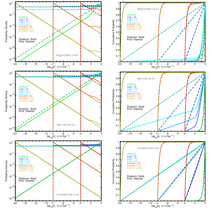
Figure 4: PDF (left) and CDF (right) of $\lambda$ for uniform, logarithmic, and inverse-uniform priors, for models Hypothetical (top), Optimistic (middle), Conservative (bottom). Curves are shown for priors with $\lambda_{\rm min}=10^{-22}\rm~{}Gyr^{-1}$, $\lambda_{\rm min}=10^{-11}\rm~{}Gyr^{-1}$, and $\lambda_{\rm min}=10^{-3}\rm~{}Gyr^{-1}$. The uniform and inverse-uniform priors lead to CDFs that are completely insensitive to the data for all three models; for the Conservative model, even the logarithmic prior is insesnsitive to the data.

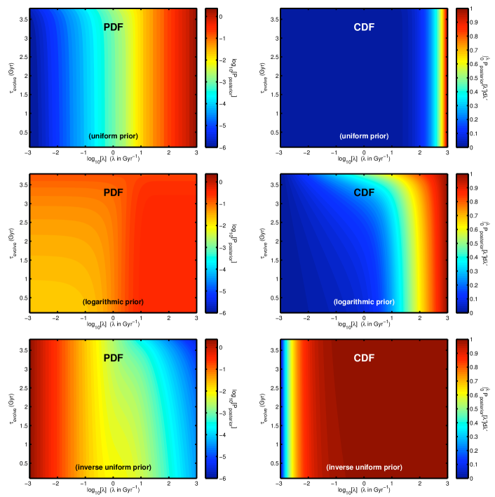
Figure 5: The influence of $\delta t_{\rm evolve}$. Uniform prior (top), logarithmic prior (middle), and inverse-uniform prior (bottom). PDF (left) and CDF (right). Aside from $\delta t_{\rm evolve}$, parameters are set to the Optimistic model with $\lambda_{\rm min}=10^{-3}\rm~{}Gyr^{-1}$ in the logarithmic and inverse-uniform cases.