Higher order Laguerre–Gauss mode degeneracy in realistic, high finesse cavities

Abstract

Higher order Laguerre–Gauss (LG) beams have been proposed for use in future gravitational wave detectors, such as upgrades to the Advanced LIGO detectors and the Einstein Telescope, for their potential to reduce the effects of the thermal noise of the test masses. This paper details the theoretical analysis and simulation work carried out to investigate the behaviour of LG beams in realistic optical setups, in particular the coupling between different LG modes in a linear cavity. We present a new analytical approximation to compute the coupling between modes, using Zernike polynomials to describe mirror surface distortions. We apply this method in a study of the behaviour of the LG₃₃ mode within realistic arm cavities, using measured mirror surface maps from the Advanced LIGO project. We show mode distortions that can be expected to arise due to the degeneracy of higher order spatial modes within such cavities and relate this to the theoretical analysis. Finally we identify the mirror distortions which cause significant coupling from the LG₃₃ mode into other order 9 modes and derive requirements for the mirror surfaces.

I introduction

The sensitivities of second generation gravitational wave detectors such as Advanced LIGO and Advanced Virgo are expected to be limited by the thermal noise of the test masses within a significant range of signal frequencies around 100 Hz Rowan05 . To reach even better sensitivities, it has been proposed to use laser beams with an intensity pattern other than that of the fundamental Gaussian beam to reduce the effects of this thermal noise Vinet07 ; Mours06 . A beam whose intensity is distributed more homogeneously over the mirror surface, for the same clipping losses, benefits from a more effective averaging over the mirror surface distortions caused by thermal effects Vinet09 . The specific advantage of using higher order LG modes, as opposed to mesa Ambrosio03 and conical Bondarescu08 beams, is that they are compatible with spherical mirrors as currently used in GW detectors and other high precision optical setups. Research into the potential of the LG₃₃ mode in gravitational wave detectors has been carried out using numerical simulations and table-top experiments Chelkowski09 ; Fulda10 . The sensing and control signals for an LG₃₃ beam were found to perform as well as for the fundamental mode in all aspects examined and the LG₃₃ behaved as expected in short linear and triangular optical cavities. However, an optical cavity resonant for a higher–order Gaussian mode is degenerate so that a number of modes can resonate at the same time. This is a fundamental difference to a well designed cavity for the fundamental Gaussian mode, in which any resonant enhancement of other modes can be suppressed. This degeneracy can potentially cause additional optical losses. Simulations have shown that the use of the LG₃₃ beam, compared to the fundamental mode, LG₀₀, could result in a significant contrast defect at the dark fringe Miller ; Galimberti ; Yamamoto . It is the aim of this paper to investigate how mirror surface distortions affect the purity of an LG₃₃ beam in high finesse cavities, by analytical calculation and numerical simulation. We will focus on the direct coupling from a distorted mirror and how this affects the mode content in a linear cavity, with our final aim to produce specifications for the mirror surfaces.

II Representing mirror surface distortions and LG modes

II.1 Mirror surface maps

Ideally the mirrors in gravitational wave detectors should be perfectly smooth with a radius of curvature matching that of the incident beam. However, real mirrors deviate from a perfect surface, altering the beams which interact with them. If a beam $U(x,y,z)$ is incident on a distorted surface described by $Z(x,y)$ and uniform reflectivity $r$, then the reflected beam is given by:

$$U_{ref}(x,y,z)=U(x,y,z)\ r\exp{(i2kZ(x,y))},$$ (1)

Fig. 1 illustrates this effect.

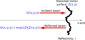
Figure 1: A diagram illustrating the phase shift introduced when a beam is reflected from a distorted mirror surface with reflectivity $r$. The surface $Z(x,y)$ is defined as a height field across a plane perpendicular to the optical axis along $z$.

In order to investigate the effects of surface distortions measured mirror surface maps can be used. The term mirror map refers to an array of data detailing the optical properties of a mirror, often its surface height in nanometers. This data can be used to represent realistic mirrors in numerical simulations of gravitational wave detectors. Mirror maps have been produced from uncoated Advanced LIGO mirror substrates which represent the best mirror surfaces of this kind currently available. In the following we have made use of one such map, the surface map of the substrate ETM08 ETM08 . The deviation of this map surface from a perfectly spherical surface with radius of curvature 2249.28 m is shown in Fig. 2. This substrate shows an RMS surface figure error of 0.523 nm.

II.2 Zernike polynomials

Zernike polynomials are well suited for the purposes of describing mirror surface distortions. Zernike polynomials can be used to describe classical distortions such as tilts and curvatures Zernike . They are a complete set of functions which are orthogonal over the unit disc and defined by radial index, $n$, and azimuthal index, $m$, with $n\geq m\geq 0$. For any index $m$ we have one odd and one even polynomial Wolf :

$$\begin{array}[]{ll}Z_{n}^{+m}(\rho,\phi)=A_{n}^{+m}\ \cos(m\phi)R_{n}^{m}(\rho)&\mbox{even polynomial}\\ \\ Z_{n}^{-m}(\rho,\phi)=A_{n}^{-m}\ \sin(m\phi)R_{n}^{m}(\rho)&\mbox{odd polynomial}\\ \end{array}$$ (2)

where $\rho$ is the normalised radial coordinate, $\phi$ is the azimuthal angle, $A_{n}^{\pm m}$ is the amplitude and $R_{n}^{m}(\rho)$ is the radial function. The radial function is given by the following sum:

$$R_{n}^{m}(\rho)=\sum_{h=0}^{\frac{1}{2}(n-m)}\frac{(-1)^{h}(n-h)!}{h!\left(\frac{1}{2}(n+m)-h\right)!\left(\frac{1}{2}(n-m)-h\right)!}\rho^{n-2h}$$ (3)

for $n-m$ even and 0 otherwise. This gives $n+1$ non-zero Zernike polynomials for each value of $n$ (for $m=0$ the odd polynomial is zero). Fig. 3 shows the surfaces described by the Zernike polynomials corresponding to orders (n) 0 to 4. The lower order polynomials represent some common optical distortions, some of which are summarised in table 1.

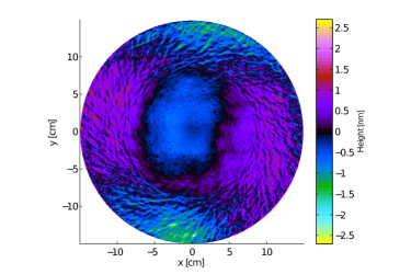
Figure 2: A surface plot of the mirror map ETM08 corresponding to the surface heights of an Advanced LIGO end test mass. The curvature has been fitted and removed from the map data.

$n$	$m$	Common name
0	0	Offset
1	$\pm 1$	Tilt in $x$/$y$ direction
2	0	Curvature
2	$\pm 2$	Astigmatism
3	$\pm 1$	Coma along $x$/$y$ axis

Table 1: Summary of some common names for the lower order Zernike polynomials Zernike .

The odd polynomial describes the same surface as the even polynomial, but rotated by 90^∘. Combinations of the odd and even polynomials relate to this same distortion rotated by a given angle. The magnitude of this surface distortion can be given by the root mean squared amplitude of the polynomials:

$$A_{n}^{m}=\sqrt{\left(A_{n}^{-m}\right)^{2}+\left(A_{n}^{+m}\right)^{2}}$$ (4)

where $+$ refers to the even polynomial and $-$ refers to the odd polynomial. Any surface defined over a disc can be described by a sum of Zernike polynomials, with the higher order polynomials representing the higher spatial frequencies present in the surface.

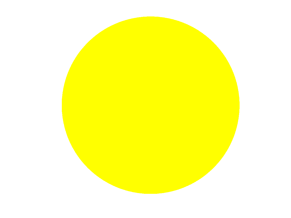
$n=0$

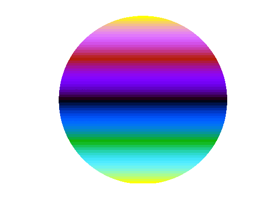
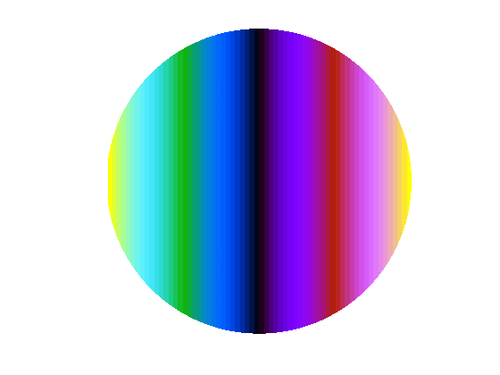
$n=1$

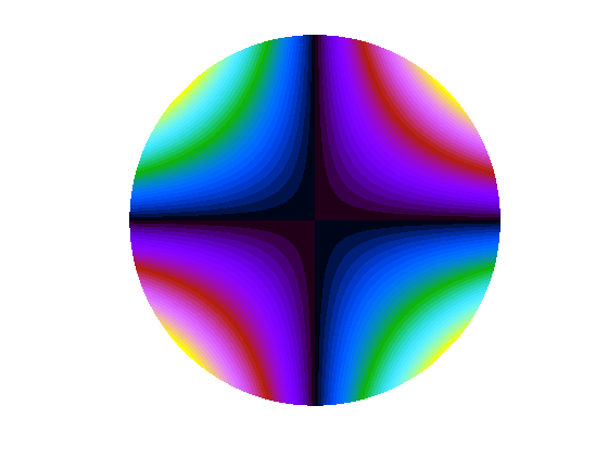
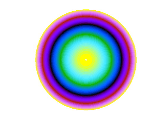
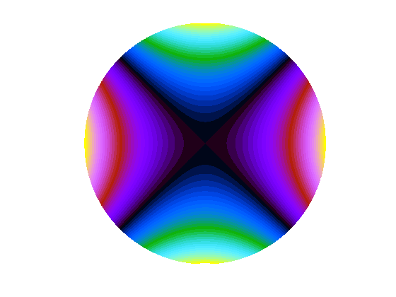
$n=2$

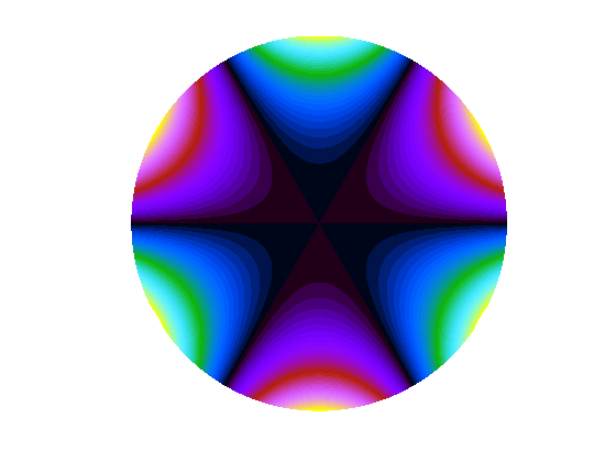
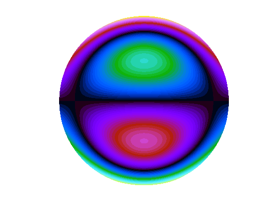
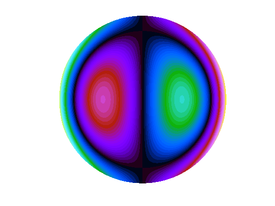
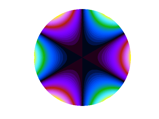
$n=3$

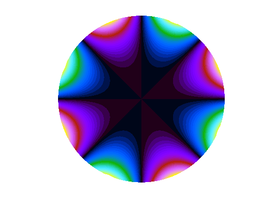
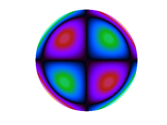
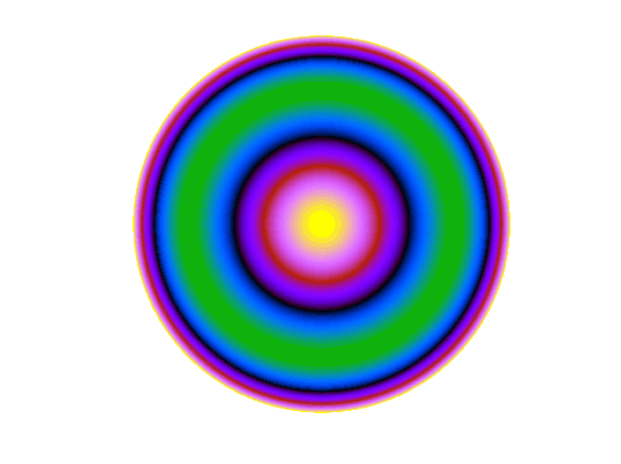
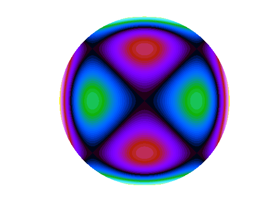
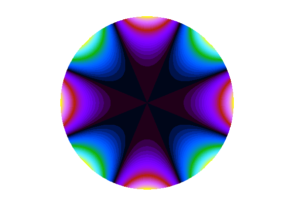
$n=4$

Figure 3: Plots of the non-zero Zernike polynomials from $n=0$ to $n=4$ with the odd polynomials with $m=-n$ on the far left and the even polynomials with $m=n$ on the far right, in steps of 2. The colour scale represents negative surface heights with greens and blues, zero with black and positive surface heights with reds and purples.

II.3 Laguerre-Gauss modes

The shape of any paraxial beam can be described as a sum of Hermite-Gauss or Laguerre-Gauss modes. The Laguerre-Gauss modes are a complete and orthogonal set of functions defined by radial index $p$ and azimuthal index $l$. The helical type of LG modes are typically given as Lasers :

$$\begin{split}U_{p,l}(r,\phi,z)={}&\frac{1}{w(z)}\sqrt{\frac{2p!}{\pi(|l|+p)!}}\exp{\left(i\left(2p+|l|+1\right)\Psi(z)\right)}\\ {}&\times\left(\frac{\sqrt{2}r}{w(z)}\right)^{|l|}L^{|l|}_{p}\left(\frac{2r^{2}}{w^{2}(z)}\right)\\ {}&\exp{\left(-\frac{ikr^{2}}{2R_{c}(z)}-\frac{r^{2}}{w^{2}(z)}+il\phi\right)}\end{split}$$ (5)

where $k$ is the wavenumber, $w(z)$ is the beam spot size parameter, $\Psi(z)$ is the Gouy phase and $R_{c}(z)$ is the radius of curvature of the beam. $L^{|l|}_{p}(x)$ refer to the associated Laguerre polynomials. When considering these beams in cavities we note that the resonance conditions for these beams differ from that of a plane wave due to the $(2p+|l|+1)\Psi(z)$ phase shift. The order of an LG mode is given by $2p+|l|$ and modes with the same order will acquire the same round trip phase shift whilst circulating in a cavity. Therefore the cavity is degenerate for LG modes of the same order.

The effects of mirror surface distortions on the shape of a reflected beam can be described in terms of coupling between LG modes. When a perfectly aligned Gaussian beam is reflected by a perfectly spherical mirror with the radius of curvature of the mirror matching that of the beam’s phase front, the shape of the reflected beam is identical to the shape of the incident beam, or, in other words, the mode composition has not changed. However, if the mirror surface is distorted the reflected beam will generally have a different mode composition. The coupling from an incident mode (indices $p$ and $l$) impinging on a completely reflecting surface $Z$ into a mode (indices $p^{\prime}$ and $l^{\prime}$) in the reflected beam can be described by a coupling coefficient Bayer-Helms ; Freise10 :

$$k_{p,l,p^{\prime},l^{\prime}}^{Z}=\int_{S}U_{p,l}\exp{\left(2ikZ\left(r,\phi\right)\right)}U^{*}_{p^{\prime},l^{\prime}}$$ (6)

$Z$ describes the surface height of the mirror and $S$ describes an infinite plane perpendicular to the optical axis.

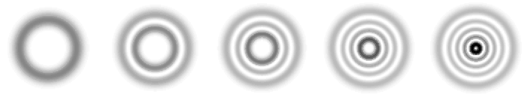
Figure 4: Plots of the intensity distributions of the order 9 helical Laguerre–Gauss modes. From left to right: LG_0±9, LG_1±7, LG_2±5, LG_3±3 and LG_4±1.

Currently the fundamental mode, LG₀₀, is used in gravitational wave detectors. Investigations have shown that mirror surface distortions have little effect on the beam purity when LG₀₀ is used. The presence of mirror surface distortions introduces modes into the detectors other than the input mode, but since LG₀₀ is the only mode of order 0 any coupling out this mode will result in modes of a different order, which will be suppressed in the cavities. The LG₃₃ mode is one of several modes of order 9. In total there are 10 order 9 modes; LG_0,±9, LG_1,±7, LG_2,±5, LG_3,±3 and LG_4,±1 (Fig. 4). These modes will be resonant in the arm cavities of the detectors, potentially resulting in a large proportion of the circulating power being in modes other than LG₃₃. The distortions present in the mirrors in each arm cavity will be different and so the mode content in each arm will differ, resulting in a larger contrast defect at the main beam splitter.

III Analytical description of mode coupling via mirror surface distortions

Using Zernike polynomials as a description of mirror surface distortions we can look at the coupling between Laguerre–Gauss modes analytically. The coupling between different Laguerre-Gauss modes when the surface is described by a particular Zernike polynomial is given by:

$$k^{n,m}_{p,l,p^{\prime},l^{\prime}}=\int_{S}U_{p,l}\exp{\left(2ikZ_{n}^{m}\right)}U^{*}_{p^{\prime},l^{\prime}}$$ (7)

In order to simplify the integral we use the fact that when $kZ$ is small we can approximate:

$$\exp{(2ikZ)}\approx 1+2ikZ$$

The amplitudes of the Zernike polynomials in the mirrors used in gravitational wave detectors are not expected to exceed 10 nm. With a wavelength of 1064 nm we have $2kZ\approx 0.1$ and so the approximation should be suitable for this investigation. We are concerned with coupling into other modes, not back into the input mode, so the equation to solve becomes:

$$k^{n,m}_{p,l,p^{\prime},l^{\prime}}=\int_{0}^{2\pi}\int_{0}^{R}U_{p,l}U^{*}_{p^{\prime},l^{\prime}}(2ikZ_{n}^{m})rdrd\phi$$ (8)

due to the orthogonal properties of LG modes.

Both the Zernike polynomials and the Laguerre-Gauss modes can be easily separated into their angular and radial parts. The angular function to integrate is:

$$\exp{(i\phi(l-l^{\prime}))}\begin{array}[]{ll}\cos{(m\phi)}&\ \ \ \mbox{even polynomial}\\ \sin{(m\phi)}&\ \ \ \mbox{odd polynomial}\\ \end{array}$$

Considering the even Zernike polynomial we obtain:

$$\begin{array}[]{c}\displaystyle\int_{0}^{2\pi}e^{i\phi(l-l^{\prime})}\frac{e^{im\phi}+e^{-im\phi}}{2}d\phi=\\ \\ \displaystyle\left[\frac{e^{i\phi(l-l^{\prime}+m)}}{2i(l-l^{\prime}+m)}+\frac{e^{i\phi(l-l^{\prime}-m)}}{2i(l-l^{\prime}-m)}\right]^{2\pi}_{0}\\ \end{array}$$

As the integral is evaluated over the entire unit disc and $e^{i0}=e^{iN\times 2\pi}=1$, where $N$ is an integer, the integral is equal to 0. The only combination of Zernike polynomials and Laguerre-Gauss beams to give a non-zero result occurs when one of the exponentials disappears before the integration takes place. This occurs when we have:

$$m=|l-l^{\prime}|$$ (9)

The same condition also gives the only non-zero results for the odd Zernike polynomials. This is a very interesting result as it suggests that surfaces described by Zernike polynomials will only cause significant coupling from one LG mode to another if the Zernike azimuthal index is equal to the difference between the azimuthal indices of the two modes. This requirement for $m$ also gives the minimum order ($n$) of Zernike polynomial required to produce significant coupling, as $m\leq n$.

Using this condition we can integrate with respect to $\phi$. The integrals were found to be $\pi$ for the even Zernike polynomials and $\pm i\pi$ for the odd polynomials, depending on the sign of $(l-l^{\prime})$. The final equation is given by:

$$\begin{split}k_{p,l,p^{\prime},l^{\prime}}^{n,m}={}&A_{n}^{m}k\sqrt{p!p^{\prime}!(p+|l|)!(p^{\prime}+|l^{\prime}|)!}\\ {}&\times\left|\sum_{i=0}^{p}\sum_{j=0}^{p^{\prime}}\sum_{h=0}^{\frac{1}{2}(n-m)}\frac{(-1)^{i+j+h}}{(p-i)!(|l|+i)!i!}\right.\\ {}&\times\frac{1}{(p^{\prime}-j)!(|l^{\prime}|+j)!j!}\frac{(n-h)!}{(\frac{1}{2}(n+m)-h)!}\\ {}&\left.\times\frac{1}{\left(\frac{1}{2}(n-m)-h\right)!h!}\frac{1}{X^{\frac{1}{2}(n-2h)}}\right.\\ {}&\left.\times\ \gamma(i+j-h+\frac{1}{2}(|l|+|l^{\prime}|+n)+1,X)\ \right|\\ \end{split}$$ (10)

where $X=\frac{2R^{2}}{w^{2}}$, $R$ is the Zernike radius and $w$ is the beam radius, and $\gamma$ is the lower incomplete gamma function. The full derivation is given in Appendix A.

In our approximation of the coupling coefficients we only consider the magnitude of the coefficients. However, the real coefficients have both real and imaginary parts indicating that there is some phase shift caused by the distortions. Therefore, when considering the coupling from a surface in terms of the coupling from the individual polynomials making up the surface we also need to consider the phase shifts. The largest possible coupling from a surface occurs when all the individual Zernike couplings have the same phase and therefore the magnitude of the coupling is equal to the sum of the individual couplings.

IV Analysis of coupling into order 9 modes

We want to verify the results of the analytical description of the coupling coefficients. Using the condition for significant coupling outlined previously in Sec. III we can identify the azimuthal Zernike indices which will cause a large amount of coupling from LG₃₃ into the other order 9 modes. These are summarised in table 2. Because $m\leq n$ this condition for the azimuthal index also tells us the lowest order ($n$) Zernike polynomial required to cause a large amount of coupling from the LG₃₃ beam into each of the other order 9 modes.

$m$	2	2	4	4	6	6	8	10	12
$U_{p,l}$ mode	2, 5	4, 1	1, 7	4,-1	0, 9	3,-3	2,-5	1,-7	0,-9

Table 2: The azimuthal index ($m$) of the Zernike polynomial required to achieve significant coupling from an LG₃₃ incident beam into the other order 9 modes.

Higher order Zernike polynomials represent higher order spatial frequencies, which generally have smaller amplitudes in the mirror surfaces. Therefore we would expect the coupling caused by higher order polynomials, such as into LG_1-7 and LG_0-9, to be smaller than those caused by lower order polynomials. We would also expect the polynomials with $m=2$, 4 and 6 to have a large effect on the beam purity as they each couple from LG₃₃ into two other order 9 modes.

Using Matlab the original integration (Eq. 7) was performed numerically, computing the coupling occurring from a mirror surface defined completely by a single Zernike polynomial. This particular example shows the results for Z${}_{4}^{4}$, in which we expect a large coupling from LG₃₃ into LG₁₇ and LG_4-1 (table 2) and much less coupling into other order 9 modes. The coupling coefficients between the LG₃₃ beam and all the other order 9 modes were calculated. The numerical integration was carried out for a range of $\frac{w}{R}$ and the results, for a polynomial amplitude of 1 nm, are summarised in Fig. 5.

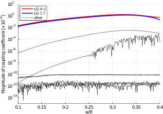
Figure 5: Plots of the coupling coefficients for different order 9 LG modes when an LG₃₃ beam is incident on a surface described by the Zernike polynomial Z${}_{4}^{4}$. The amplitude of the coefficients is plotted against the ratio of the beam radius, $w$, and the Zernike radius, $R$. These plots show numerical results for the coefficients without any approximation. The coefficients for LG_4-1 and LG₁₇ are significantly larger than those of the other modes.

In this plot the two largest coupling coefficients over this range of $\frac{w}{R}$ correspond to LG_4-1 and LG₁₇. The coefficients for the other LG modes are significantly smaller. These results agree with our predictions.

Fig. 6 shows a comparison of the analytical results from Eq. 10 with the numerical results. Here only the coupling coefficients for LG_4-1 and LG₁₇ are plotted as the analytical approach gives 0 for $m\neq|l-l^{\prime}|$. Over this range the two sets of numbers match up very well and we consider this a good confirmation of the analytical approximation.

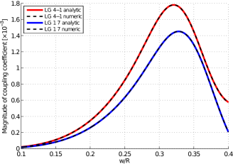
Figure 6: A plot showing the coupling into the LG_4-1 and LG₁₇ modes from an LG₃₃ beam incident on a surface described by the Zernike polynomial Z${}_{4}^{4}$. The results are plotted against the relative beam radius on the mirror, $\frac{w}{R}$. The results from an analytical approximation and a numerical integration method are plotted.

IV.1 Beam size and Zernike order

Figs. 5 and 6 seem to suggest that the coupling coefficients also depend on the beam size relative to the radius of the Zernike polynomial, or mirror radius. However, this ratio is typically not a free parameter. For a good reduction in thermal noise a large beam radius is desirable. An upper limit for the beam width can be derived from optical loss due to beam clipping. This so-called clipping loss refers to the power lost over the mirror edges given by Chelkowski09 :

$$l_{\mbox{clip}}=1-\int_{S}\left|U_{p,l}\right|^{2},$$ (11)

where the integral represents the normalised power reflected by a perfect mirror of finite size (see Appendix B). In gravitational wave detectors the clipping loss should be lower than 100 ppm (parts per million) and often an arbitrary requirement of 1 ppm is used during the interferometer design phase. This yields an optimal beam radius of $0.232\,R$ ($R$ being the mirror radius) for an LG₃₃ beam. A clipping loss of 100 ppm instead leads to an optimal beam radius of $0.255\,R$.

V Cavity simulations with Advanced LIGO mirror maps

We want to investigate how the degeneracy of the order 9 modes affects the purity of an LG₃₃ mode in high finesse cavities. The aim of this investigation is to assess the effects of higher-order mode degeneracy and derive requirements for the mirror surfaces which would result in an acceptably high LG₃₃ beam purity. The Advanced LIGO cavities consist of two curved mirrors; the input test mass (ITM) and the end test mass (ETM) separated by an arm length of approximately 4 km (Fig. 7). The design properties of these mirrors are summarised in table 3 ITM ; ETM , giving a high finesse of 450.

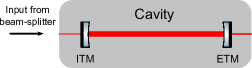
Figure 7: The optical layout of an Advanced LIGO arm cavity. Light from the beam-splitter is incident on the flat anti-reflective surface of the ITM. The light circulates between the two highly reflective, curved surfaces of the ITM and ETM. Light is transmitted by the cavity through the ETM.

Mirror	ITM	ETM
$R_{a}$	20 ppm	500 ppm
$L_{a}$	1 ppm	1 ppm
$T_{h}$	0.014	5 ppm
$L_{h}$	0.3 ppm	0.3 ppm

Table 3: Optical properties of the mirrors designed for the Advanced LIGO arm cavities. The two mirrors have a design thickness of 200 mm and index of refraction of 1.45. $R$, $T$ and $L$ refer to the reflectivity, transmission and loss of power at the mirror. $a$ and $h$ refer to the anti-reflective and highly reflective coated surfaces of each mirror.

To simulate mirror surface distortions we used mirror maps measured from uncoated mirror substrates produced for Advanced LIGO . However, the Advanced LIGO cavities were not designed to be compatible with the LG₃₃ mode. The LG₃₃ mode is more spatially extended than the LG₀₀ mode, and so experiences a larger clipping loss at the mirrors for a given beam spot size value. For the Advanced LIGO cavity parameters, the clipping loss for the LG₃₃ mode is much larger than acceptable, at around 35%. It was therefore necessary to adjust the cavity length to bring the LG₃₃ clipping to a level that allowed us to carry out a meaningful investigation. Using a cavity length of 2802.9 m we achieve similar clipping losses to those experienced by LG₀₀ in the original cavities, for the 30 cm aperture represented by the mirror maps. The results from this optical setup should be representative of longer cavities with larger mirrors. The simulated cavity parameters are summarised in table 4.

Parameter	ITM Rc	ETM Rc	Cavity length
Value [m]	-1934	2245	2802.9

Table 4: Cavity parameters for simulations of Advanced LIGO style arm cavities AdLIGO . The length of the cavity was reduced from the original length of 3994.5 m to prevent a large clipping loss when using LG₃₃ beams.

V.1 Laguerre-Gauss mode purity with Advanced LIGO mirror maps

For the purposes of this investigation the mirror map corresponding to the Advanced LIGO end test mass ETM08 was used; see Fig. 2. To predict the direct couplings from this mirror we look at the Zernike polynomials representing the mirror surface. This is achieved by performing a convolution between the surface defined by the mirror map and the different Zernike polynomials:

$$\int_{S}Z_{map}\cdot Z_{n}^{m}=A_{n}^{m}\int_{S}Z_{n}^{m}\cdot Z_{n}^{m}$$ (12)

where $Z_{map}$ is the surface defined by the mirror map and $A_{n}^{m}$ is the amplitude of the corresponding Zernike polynomial in the surface. The convolution was performed for all Zernike polynomials with $n\leq 30$. The polynomials which cause significant coupling into the other order 9 modes ($m=2$, 4,$\dots$12) are summarised in table 5. Here the polynomials are ranked in order of the power they couple into the other order 9 modes when an LG₃₃ beam is reflected from a surface described by the polynomial.

Z${}_{n}^{m}$ polynomial	2, 2	4, 2	4, 4	6, 2	10, 8	other
$A_{n}^{m}$ [nm]	0.908	0.202	0.213	0.124	0.116	-
Power [ppm]	4.66	0.331	0.0431	0.0099	0.0059	$<$ 0.005

Table 5: Zernike polynomials present in the Advanced LIGO mirror map ETM08 which cause significant coupling from LG₃₃ into the other order 9 LG modes ($m=2$, 4,$\dots$12). The power coupled from LG₃₃ into the other order 9 modes by reflection from surfaces described by the individual polynomials is included, calculated from a coupling approximation.

From this we can suggest which order 9 LG modes will have significant amplitudes in the simulated cavity. The two polynomials which cause the largest individual power couplings have $m=2$. The astigmatism (Z${}_{2}^{2}$) in particular extracts a large amount of power from LG₃₃. Therefore, we would expect the LG₄₁ and LG₂₅ modes to have relatively large amplitudes in the cavity as the $m=2$ polynomials cause significant coupling into these modes.

The cavity defined in Sec. 7 was simulated using the interferometer simulation tool Finesse  Finesse ; Finesse2 . An input beam of pure LG₃₃ was used with the ETM08 mirror map applied to the end mirror and a perfect input mirror. The cavity was tuned to be on resonance for the LG₃₃ mode and the beam circulating in the cavity was detected. A plot of the circulating field is shown in Fig. 8.

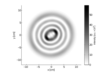
Figure 8: A plot of the field circulating in a simulated high finesse cavity. In the simulation the Advanced LIGO mirror map ETM08 is applied to the end test mass and a pure LG₃₃ beam is injected into the cavity.

The purity of an LG mode, $U_{p,l}$, in a given beam $U$ is defined as $|c_{p,l}|^{2}$ where Chu :

$$c_{p,l}=\int_{S}U\ U_{p,l}^{*}$$ (13)

The plot in Fig. 8 (compared with the plot of LG₃₃ in Fig. 4) suggests that the circulating beam now contains modes other than LG₃₃. The purity of the LG₃₃ beam in this simulated cavity was found to be 88.6%. The power in the different modes present in the circulating field are summarised in table 6.

$U_{p,l}$ mode	3, 3	4, 1	2, 5	4,-1	1, 7	other
$m_{SC}$	-	2	2	4	4	-
Power (%)	88.6	5.70	5.02	0.333	0.313	$<$ 0.05

Table 6: The power in the LG modes circulating in a cavity simulated with Finesse with an LG₃₃ input beam and the Advanced LIGO mirror map ETM08. $m_{SC}$ refers to the azimuthal index of the Zernike polynomial required to cause significant coupling from LG₃₃ to the given mode.

The results of the decomposition show that the surface distortions of the end mirror cause significant coupling into other LG modes, particularly the other order 9 modes. The distortions also cause coupling into modes of other orders, but these are not resonant at the same cavity tuning as the LG₃₃ mode and so are strongly suppressed.

Other than LG₃₃ the two largest modes in the cavity are LG₄₁ (5.7 %) and LG₂₅ (5.0 %). This agrees with the predictions made by studying the Zernike content of the ETM08 mirror map (table 5). LG_4-1 and LG₁₇ also have relatively large amplitudes in the cavity. This may be due to the direct coupling out of the LG₃₃ caused by the Z${}_{4}^{4}$ polynomial. However, the LG_4-1 and LG₁₇ modes can also be strongly coupled out of the LG₄₁ and LG₂₅ modes via $m=2$ polynomials, further contributing to the effect these polynomials have on the purity of the beam. Overall the coupling process in a cavity is complicated by these multiple cross-couplings, but the results of this simulation suggest that the direct coupling from a mirror surface is the dominant effect on the mode content of the circulating beam. A theoretical understanding of the direct coupling has therefore allowed us to make valid predictions about the resulting mode content.

V.2 Frequency splitting

The presence of mirror surface distortions not only causes coupling between LG modes but introduces additional phase shifts of the modes. This results in slight shifts of the resonance frequency of individual modes. These shifts in resonance frequency depend on the particular mode and so modes of the same order will be resonant at slightly different frequencies. Thus the mode degeneracy can be broken. We will refer to this effect as frequency splitting. For the frequency splitting to be effective the shifts in resonance frequency must be larger than the cavity bandwidth in order to separate the resonance peaks of the different order 9 modes.

Using the ETM08 mirror map the high finesse cavity defined in Sec. 7 was simulated. The beam circulating in the cavity was detected as the laser frequency was tuned around the cavity resonance. The maximum power of the order 9 modes in the cavity and the difference in their resonance frequencies is summarised in table 7. The frequency splitting is of the order of 10 Hz, smaller than the cavity bandwidth of 120 Hz and so is not sufficient to completely break the degeneracy. The result is 10 quasi-degenerate modes. The resonance frequencies are slightly different and so when the cavity is tuned to the resonance of the LG₃₃ mode the other modes will be slightly suppressed. However, the frequency splitting is small and therefore these modes will still have relatively large amplitudes in the cavity. The coupling into order 9 modes is therefore still the dominant effect on the mode purity.

$U_{p,l}$ mode	3, 3	4, 1	2, 5	4, -1	1, 7	3, -3	0, -9	2, -5	0, 9	1, -7
Power [W]	221.8	14.38	12.62	0.865	0.802	0.102	0.038	0.038	0.032	0.001
Frequency [Hz]	0	1.3	0.7	7.0	6.6	7.6	-7.3	-16.1	-14.8	9.3

Table 7: A summary of the power in each order 9 mode in a simulated cavity where the mirror map ETM08 is applied to the end mirror and the input mode is LG₃₃. The frequency is tuned around the cavity resonance and the difference in resonance frequency, compared to LG₃₃, is included for each mode.

V.3 Laguerre-Gauss mode purity with improved mirror maps

We want to find ways in which the mirror maps could be improved for the specific application of the LG₃₃ beam. By considering the mirror surfaces analytically it appears that reducing the astigmatism for this particular map could improve the purity of LG₃₃ in our simulated cavity. To demonstrate this the astigmatism was removed from the ETM08 mirror map. The cavity was then simulated with this processed map, with the resulting circulating field detected and decomposed in to LG modes. The circulating beam is plotted in Fig. 9. Simply comparing this plot with the original circulating beam (Fig. 8) suggests that the purity of the field has increased. The LG content of the beam is summarised in table 8. The purity of the circulating LG₃₃ beam is now 99.5%, a significant improvement from the original results.

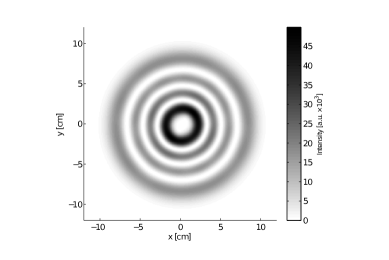
Figure 9: A plot of the field circulating in a cavity simulated with an input mode of pure LG₃₃ and the Advanced LIGO ETM08 mirror map, with astigmatism removed.

$U_{p,l}$ mode	3, 3	4, 1	2, 5	1, 7	4,-1	0,-9	other
$m_{SC}$	-	2	2	4	4	12	-
Power [%]	99.5	0.231	0.208	0.0524	0.0165	0.0137	$<$ 0.01

Table 8: The power in the LG modes circulating in a simulated cavity. The cavity was simulated with an LG₃₃ input beam and with the ETM08 mirror map with astigmatism removed. $m_{SC}$ refers to the azimuthal index of the Zernike polynomial required to cause significant coupling from LG₃₃ to the given mode.

The results of the decomposition show that the power in both the LG₄₁ and LG₂₅ modes has decreased significantly, as predicted. The power in the other modes has also noticeably decreased. This result suggests that the astigmatism is a major factor in coupling from the LG₃₃ mode, not only for its direct coupling into LG₂₅ and LG₄₁ but for the coupling from these new modes into other modes of order 9. For this setup we can conclude that the astigmatism should be limited in the mirror surfaces to reduce the problems caused by higher order mode degeneracy.

V.4 Mirror requirements for LG₃₃

In order to use LG₃₃ in GW detectors we require certain Zernike polynomials in the mirrors to be smaller than in the current state of the art mirrors, in order to achieve an acceptable beam purity in the cavity. Here we investigate the direct coupling from ETM08 and suggest limits to the amplitudes of specific polynomials in the mirror surfaces, presenting an Advanced LIGO mirror map adapted for the use of LG₃₃.

Using our theoretical analysis we can identify the particular Zernike polynomials to reduce in the mirrors. We have already seen that the Zernike polynomials with odd values of $n$ and with $m>12$ don’t have a large effect on the purity. To assess the other polynomials we use Eq. 10 to approximate the coupling into order 9 modes caused by the polynomials in the ETM08 mirror map, for the optical setup defined in Sec. 7. For each order 9 LG mode the coupling was calculated for the Zernike polynomials with $n=2$, 4 $\dots$30 and with $m$ required to give significant coupling. Fig. 10 represents these coupling coefficients.

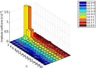
Figure 10: A bar chart showing the coupling, $k_{p,l,p^{\prime},l^{\prime}}^{n,m}$, into the order 9 modes when an LG₃₃ beam is incident on a surface described by the Zernike polynomial with $m$ required to cause significant coupling. The Zernike amplitudes correspond to those in the ETM08 mirror map.

This chart shows that the largest couplings occur from Z${}_{2}^{2}$, into LG₂₅ and LG₄₁, as previously suggested. There is also some strong coupling from Z${}_{4}^{2}$ and Z${}_{4}^{4}$. The other couplings are significantly smaller. Therefore, the first step in modifying the mirrors for LG₃₃ is to limit these 3 polynomials to give similar couplings to the higher order polynomials.

Another plot illustrating the coupling from this map is shown in Fig. 11. In this plot the maximum possible coupling from the ETM08 mirror map is estimated using our analytical approximation. For each order 9 mode the sum of the coupling is calculated for all Zernike polynomial orders smaller than $n$. The plot illustrates the magnitude of the direct coupling expected as we include higher order Zernike polynomials in our model.

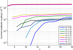
Figure 11: Plots showing an approximation of the coupling from LG₃₃ into the other order 9 LG modes from the ETM08 mirror map as higher order ($n$) Zernike polynomials are included in our model. The sum of the coupling from polynomials with order $\leq n$ are plotted for each mode.

Fig. 11 can be used to illustrate how this particular map, ETM08, should be adapted for LG₃₃. The coupling into LG₂₅ and LG₄₁ is around 10 times greater than any other coupling. The coupling into these two modes is also not significantly increased by including the higher order modes. Therefore, limiting the lower order polynomials with $m=2$ will greatly reduce the coupling into these two modes and the overall coupling into order 9 modes. From this plot we conclude that the overall coupling into order 9 modes can be reduced by around a factor of 10 by reducing the lower order polynomials. Reducing the coupling further will involve limits on multiple polynomials.

By assessing the direct coupling from ETM08 we can set requirments for the lower order Zernike polynomials. When an LG₃₃ beam is incident on the ETM08 mirror map in our setup the reflected beam is predominantly LG₃₃. However, we find 31 ppm (parts per million) of the power is now in other modes, with 6.8 ppm in the other order 9 modes. Table 5 shows the power coupled from surfaces described by the polynomials present in the ETM08 map, from LG₃₃ into the other order 9 modes. For this map we consider the polynomials causing a large amount of coupling as those coupling more than 0.01 ppm into the order 9 modes; Z${}_{2}^{2}$, Z${}_{4}^{2}$ and Z${}_{4}^{4}$. For LG₃₃ we require these polynomials to be limited in the mirror surfaces. The requirements for these polynomials were calculated to give power couplings of 0.01 ppm into the other order 9 modes and are summarised in table 9.

$Z_{n}^{m}$ polynomial	2, 2	4, 2	4, 4
Amplitude [nm]	0.042	0.035	0.100

Table 9: A summary of the amplitude requirements for the Zernike polynomials required to give individual couplings of 0.01 ppm from LG₃₃ into the other order 9 modes in the ETM08 mirror map.

These amplitude limits were applied to the ETM08 mirror map, resulting in coupling of 19 ppm into modes other than LG₃₃ and 0.043 ppm into the other order 9 modes. The cavity defined in Sec. 7 was simulated with this limited map, resulting in 815 ppm impurity in the circulating beam. This is a very good improvement on the original impurity of 0.114, illustrating that a high beam purity is achievable with these mirror requirements. To achieve an even higher beam purity will involve reducing the amplitudes of these polynomials further, as well as additional Zernike requirements.

VI Conclusion

We have investigated the coupling which occurs when Laguerre-Gauss modes are incident on a mirror with surface distortions. Taking an analytical approach we used Zernike polynomials to represent mirror surface distortions and derived an approximate equation for the significant coupling when an LG mode is reflected from a surface defined by a particular Zernike polynomial. This derivation resulted in a condition for significant coupling, $m=|l-l^{\prime}|$, where $m$ is the azimuthal index of the Zernike polynomial and $l$ and $l^{\prime}$ are the azimuthal indices of the incident and coupled modes respectively. This is a significant result as it allows us to predict which order 9 modes will be largely coupled by particular Zernike polynomials and suggest which modes will have large amplitudes in the arm cavities

We investigated the performance of LG₃₃ in high finesse cavities by simulation with Advanced LIGO mirror maps. This illustrated the degraded purity of the circulating beam in realistic cavities due to higher order mode degeneracy. The results were then analysed by looking at the Zernike polynomials representing our example mirror map. The analysis and results were consistent with the predictions made from Eq. 10. This suggested that astigmatism was causing a significant amount of coupling, particularly into the LG₄₁ and LG₂₅ modes. This was confirmed when the cavity was simulated again with the astigmatism removed from the mirror map and we observed a dramatic increase in the LG₃₃ mode purity.

The analytical description enabled us to identify the specific Zernike polynomials which cause large couplings as well as the LG modes which would dominate as a result. Using this we were able to derive certain requirements for our example mirror map, ETM08, in terms of limits on the amplitudes of the Zernike polynomials Z${}_{2}^{2}$, Z${}_{4}^{2}$ and Z${}_{4}^{4}$ (table 9). Using this map the resulting circulating beam impurity was found to be 815 ppm, a significant reduction from the original impurity of 0.114.

This investigation has demonstrated that a high beam purity is achievable using an LG₃₃ beam when modifications are made to the low order Zernike polynomials in Advanced LIGO mirrors. Implementing the LG₃₃ beam in gravitational wave detectors will be challenging as we require very small amplitudes on these lower order polynomials. We should also consider that the example mirror surfaces considered here refer to uncoated substrates. The coating process is likely to add to the lower order features in the mirror surfaces. However, using this analytical approach we can derive specific requirements for the mirror surfaces leading to designs for suitable mirrors for these higher order beams.

Appendix A Derivation of coupling coefficients

The product of two Laguerre-Gauss modes is:

$$\begin{split}U_{p,l}U^{*}_{p^{\prime},l^{\prime}}={}&\frac{1}{w^{2}}\frac{2}{\pi}\sqrt{\frac{p!p^{\prime}!}{(|l|+p)!(|l^{\prime}|+p^{\prime})!}}\\ {}&\times\exp{\left(i\left(2p+|l|-2p^{\prime}-|l^{\prime}|\right)\Psi\right)}\\ {}&\left(\frac{\sqrt{2}r}{w}\right)^{|l|+|l^{\prime}|}L^{|l|}_{p}\left(\frac{2r^{2}}{w^{2}}\right)L^{|l^{\prime}|}_{p^{\prime}}\left(\frac{2r^{2}}{w^{2}}\right)\\ {}&\exp{\left(-\frac{2r^{2}}{w^{2}}\right)}\exp{\left(i\phi\left(l-l^{\prime}\right)\right)}\end{split}$$ (14)

The following derivation follows from Eq. 9. Currently we are concerned with the magnitude of the coupling coefficients, so we ignore any constant phase shifts and integrate with respect to $\phi$:

$$\begin{split}k^{n,m}_{p,l,p^{\prime},l^{\prime}}={}&\left|\int_{0}^{R}\frac{2}{\pi w^{2}}\sqrt{\frac{p!p^{\prime}!}{(|l|+p)!(|l^{\prime}|+p^{\prime})!}}2kA_{n}^{m}\pi R_{n}^{m}(r)\right.\\ {}&\times\left(\frac{\sqrt{2}r}{w}\right)^{|l|+|l^{\prime}|}L_{p}^{|l|}\left(\frac{2r^{2}}{w^{2}}\right)L_{p^{\prime}}^{|l^{\prime}|}\left(\frac{2r^{2}}{w^{2}}\right)\\ {}&\left.\times\exp{\left(-\frac{2r^{2}}{w^{2}}\right)}rdr\right|\\ \end{split}$$ (15)

In order to further simplify the equation the following variable substitution is made:

$$x=\frac{2r^{2}}{w^{2}}$$ (16)

and a new limit to the integral:

$$X=\frac{2R^{2}}{w^{2}}$$ (17)

where $R$ is the Zernike radius. This gives the integral:

$$\begin{split}k^{n,m}_{p,l,p^{\prime},l^{\prime}}={}&kA_{n}^{m}\sqrt{\frac{p!p^{\prime}!}{(|l|+p)!(|l^{\prime}|+p^{\prime})!}}\\ {}&\times\left|\int_{0}^{X}R_{n}^{m}(x)x^{\frac{1}{2}(|l|+|l^{\prime}|)}\right.\\ {}&\times\left.L_{p}^{|l|}(x)L_{p^{\prime}}^{|l^{\prime}|}(x)\exp{(-x)}dx\right|\end{split}$$ (18)

Substituting in the sums representing the Laguerre polynomials and the radial Zernike function as a function of $x$ gives:

$$\begin{split}k_{p,l,p^{\prime},l^{\prime}}^{n,m}={}&A_{n}^{m}k\sqrt{p!p^{\prime}!(p+|l|)!(p^{\prime}+|l^{\prime}|)!}\\ {}&\times\left|\sum_{i=0}^{p}\sum_{j=0}^{p^{\prime}}\sum_{h=0}^{\frac{1}{2}(n-m)}\frac{(-1)^{i+j+h}}{(p-i)!(|l|+i)!i!}\right.\\ {}&\times\frac{1}{(p^{\prime}-j)!(|l^{\prime}|+j)!j!}\frac{(n-h)!}{(\frac{1}{2}(n+m)-h)!}\\ {}&\left.\times\frac{1}{\left(\frac{1}{2}(n-m)-h\right)!h!}\frac{1}{X^{\frac{1}{2}(n-2h)}}\right.\\ {}&\left.\times\int_{0}^{X}x^{i+j-h+\frac{1}{2}(|l|+|l^{\prime}|+n)}\exp{(-x)}dx\right|\\ \end{split}$$ (19)

This type of integral results in the lower incomplete gamma function:

$$\gamma(a,x)=\int_{0}^{x}t^{a-1}e^{-t}dt$$ (20)

When $a$ is equal to $n$, an integer, the function is given by the following sum:

$$\gamma(n,x)=(n-1)!\left(1-e^{-x}\sum_{k=0}^{n-1}\frac{x^{k}}{k!}\right)$$ (21)

Therefore, the final equation for this approximation of the magnitude of the coupling coefficients is given by:

$$\begin{split}k_{p,l,p^{\prime},l^{\prime}}^{n,m}={}&A_{n}^{m}k\sqrt{p!p^{\prime}!(p+|l|)!(p^{\prime}+|l^{\prime}|)!}\\ {}&\times\left|\sum_{i=0}^{p}\sum_{j=0}^{p^{\prime}}\sum_{h=0}^{\frac{1}{2}(n-m)}\frac{(-1)^{i+j+h}}{(p-i)!(|l|+i)!i!}\right.\\ {}&\times\frac{1}{(p^{\prime}-j)!(|l^{\prime}|+j)!j!}\frac{(n-h)!}{(\frac{1}{2}(n+m)-h)!}\\ {}&\left.\times\frac{1}{\left(\frac{1}{2}(n-m)-h\right)!h!}\frac{1}{X^{\frac{1}{2}(n-2h)}}\right.\\ {}&\left.\times\ \gamma(i+j-h+\frac{1}{2}(|l|+|l^{\prime}|+n)+1,X)\ \right|\\ \end{split}$$ (22)

Appendix B Clipping loss

Clipping loss is given by:

$$l_{\mbox{clip}}=1-\int_{S}\left|U_{p,l}\right|^{2}$$ (23)

where the integral represents the normalised power reflected by a perfect mirror. $S$ defines an infinite plane perpendicular to the beam axis. The magnitude squared of an LG mode is:

$$\begin{split}\left|U_{p,l}\right|^{2}={}&\frac{1}{w^{2}}\frac{2p!}{\pi(|l|+p)!}\left(\frac{2r^{2}}{w^{2}}\right)^{|l|}\\ {}&\times\left(L^{|l|}_{p}\left(\frac{2r^{2}}{w^{2}}\right)\right)^{2}\exp{\left(-\frac{2r^{2}}{w^{2}}\right)}\\ \end{split}$$ (24)

where $w$ is the beam radius, $p$ and $l$ are the mode indices and $r$ is the radial position. Integrating over the surface and taking a similar approach as for the coupling coefficients we get:

$$\begin{split}l_{\mbox{clip}}={}&1-p!(p+|l|)!\sum_{m=0}^{p}\sum_{n=0}^{p}\frac{(-1)^{n+m}}{(p-n)!(p-m)!}\\ {}&\times\frac{1}{(|l|+n)!(|l|+m)!n!m!}\ \gamma(|l|+n+m+1,X)\\ \end{split}$$ (25)

where $X=\frac{2R^{2}}{w^{2}}$, $R$ is the radius of the mirror and $\gamma$ is the lower incomplete gamma function.

Appendix C Zernike composition of a mirror surface

For certain Zernike polynomials (those with non-zero $m$) their amplitudes in a surface depend on the orientation of that surface with respect to the Zernike surface. For example, consider the two polynomials responsible for astigmatism, Z${}_{2}^{\pm 2}$. The two polynomials actually describe the same shape, with one just rotated by 90 degrees with respect to the other. Therefore, rotating a surface, such as the one described by mirror map ETM08, will change the amplitudes of these two polynomials within the surface. Fig. 12 illustrates this effect. The plots show the amplitudes of the order 2 Zernike polynomials present in the ETM08 mirror surface as it is rotated. As expected the amplitude of the Z${}_{2}^{0}$ polynomial remains constant as it has no angular dependence. The amplitudes of the Z${}_{2}^{\pm 2}$ polynomials oscillate and, at a certain rotation (around 120^∘) the astigmatism of the surface is completely described by Z${}_{2}^{+2}$, and 90^∘ later completely described by Z${}_{2}^{-2}$. The root mean squared amplitude ($A_{2}^{2}$) of the polynomials remains constant.

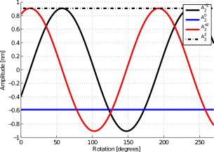
Figure 12: Plots of the amplitudes of the order 2 Zernike polynomials present in the surface described by the ETM08 Advanced LIGO mirror map as a function of the rotation of the surface.

Appendix D Analysis of Zernike approach

We have used Zernike polynomials to describe mirror surface distortions and analyse the coupling that occurs from LG₃₃ into other order 9 modes. This approach appears to be very suitable as we have been able to identify specific polynomials which extract significant amounts of power from the input mode. However, there is an alternative method used to investigate mirror surface distortions, which involves looking at the spatial frequencies present in real mirrors. In this section we compare these two methods.

To look at the spatial frequencies present in realistic mirrors we perform a 2D Fourier transform of the surface height data. The resulting spectra is then analysed and synthetic maps are created with the same spatial frequencies. This method focuses on identifying particular spatial wavelengths which cause a large degree of coupling from LG₃₃. Many synthetic maps are created and used in simulations of gravitational wave detectors. A statistical approach is then taken to determine the extent of the coupling when specific spatial frequencies are present in the mirror.

In the Zernike approach we look at the different polynomials present in mirror surface distortions. This can be thought of as equivalent to looking at the spectra of the mirror surfaces as the different polynomials represent different spatial frequencies. The plot in Fig. 13 illustrates this. The spectrum of the ETM08 Advanced LIGO mirror map is shown, along with the spectra of maps made up from the Zernike polynomials present in the ETM08 mirror. Each of the Zernike maps recreates the LIGO map with polynomials up to a certain order. The plots show that as the order of Zernike polynomials present increases the higher spatial frequencies are represented in the mirror map. This is because these higher order polynomials represent the higher order spatial frequencies. Looking at the spatial frequencies present in the Zernike polynomials we found that the frequencies depended on the order, $n$. A consequence of this is that if we just consider the spatial frequencies present in the mirror maps we will not be able to distinguish between polynomials with different $m$. As we have seen, the azimuthal index is very significant as it determines which modes are largely coupled from LG₃₃. Therefore looking at the spatial frequencies doesn’t identify the important shapes in the mirror surfaces. The Zernike approach would seem to be the most suitable as this allows us to identify the interesting polynomials and modes.

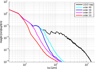
Figure 13: A plot showing the spectrum of the Advanced LIGO mirror map, ETM08 and the spectra of maps created from Zernike polynomials present in ETM08. The Zernike maps go up to a certain maximum order, recreating higher spatial frequencies with higher orders.

References

- (1) S. Rowan, J. Hough and D. Crooks, Phys. Lett. A, 347, 25 (2005)
- (2) J.-Y. Vinet, Classical Quantum Gravity, 24, 3897 (2007)
- (3) B. Mours, E. Tournefier and J.-Y. Vinet, Classical Quantum Gravity, 23, 5777 (2006)
- (4) J.-Y. Vinet, Living Rev. Relativity, 12, 1 (2009), http://www.livingreviews.org/lrr-2009-5
- (5) E. D’Ambrosio, Phys. Rev. D, 67, 102004 (2003)
- (6) M. Bondarescu, O. Kogan and Y. Chen, Phys. Rev. D, 78, 082002 (2008)
- (7) S. Chelkowski, S. Hild and A. Freise, Phys. Rev. D, 79, 122002 (2009)
- (8) P. Fulda, K. Kokeyama, S. Chelkowski and A. Freise, Phys. Rev. D, 82, 012002 (2010)
- (9) John Miller: ‘New Beam Shape with Low Thermal Noise’ (Elba 2011), http://agenda.infn.it/contributionDisplay.py?contribId=44&sessionId=19&confId=3351
- (10) M. Galimberti and R. Flaminio: ‘Mirror requirements for 3rd generation GW detectors’ (GWADW 2010), http://gw.icrr.u-tokyo.ac.jp/gwadw2010/program/2010_GWADW_Galimberti.pdf
- (11) H. Yamamoto: ‘Reduction of degenerate modes excitation in an imperfect FP cavity for LG33 beam’, LIGO-T1100220-v1, LSC (2011)
- (12) Tinsley: ‘Final Data Package ALIGO ETM-08’, LIGO-C1000486-v1, LSC (2010)
- (13) ‘Zernike Polynomials and Their Use in Describing the Wavefront Aberrations of the Human Eye’ (Stanford University, 2003) http://scien.stanford.edu/pages/labsite/2003/psych221/projects/03/pmaeda/index.html
- (14) M. Born and E. Wolf, Principles of Optics, 7th (expanded) edition, (Cambridge University Press, Cambridge, UK, 1999)
- (15) A. Siegman, Lasers (University Science Books, Sausalito, California, 1986)
- (16) A. Freise and K. Strain, Living Rev. Relativity, 13, 1 (2010), http://www.livingreviews.org/lrr-2010-1
- (17) F. Bayer-Helms, Appl. Opt., 23, (1984) 1369-1380.
- (18) Advanced LIGO Team, Tech. Rep. LIGO-E0900041-v5, LSC (2009)
- (19) Advanced LIGO Team, Tech. Rep. LIGO-E0900068-v3, LSC (2009)
- (20) Advanced LIGO Team, Tech. Rep. LIGO-T0900043-10, LSC (2009)
- (21) A. Freise: ‘Finesse 0.99.8: Frequency domain interferometer simulation software’ (2008) Finesse manual available at http://www.gwoptics.org/finesse/
- (22) A. Freise, G. Heinzel, H. Lück, R. Schilling, B. Willke and K. Danzmann, Classical Quantum Gravity, 21, (2004)
- (23) S.-C. Chu and K. Otsuka, Opt. Commun., 281, 1647 (2008)
- (24) C. Bond and A. Freise, (paper in preparation)