Influence and Dynamic Behavior in Random Boolean Networks

Abstract

We present a rigorous mathematical framework for analyzing dynamics of a broad class of Boolean network models. We use this framework to provide the first formal proof of many of the standard critical transition results in Boolean network analysis, and offer analogous characterizations for novel classes of random Boolean networks. We precisely connect the short-run dynamic behavior of a Boolean network to the average influence of the transfer functions. We show that some of the assumptions traditionally made in the more common mean-field analysis of Boolean networks do not hold in general. For example, we offer some evidence that imbalance, or expected internal inhomogeneity, of transfer functions is a crucial feature that tends to drive quiescent behavior far more strongly than previously observed.

Introduction.

Complex systems can usually be represented as a network of interdependent functional units. Boolean networks were proposed by Kauffman as models of genetic regulatory networks Kauffman (1969, 1993) and have received considerable attention across several scientific disciplines. They model a variety of complex phenomena, particularly in theoretical biology and physics Harris et al. (2002); Shmulevich and Kauffman (2004); Moreira and Amaral (2005); Aldana and Cluzel (2003); Kauffman et al. (2003); Shmulevich et al. (2003).

A Boolean network ${\cal N}$ with $n$ nodes can be described by a directed graph $G=(V,E)$ and a set of transfer functions. We use $V$ and $E$ to denote the sets of nodes and edges respectively, and denote the indegree of node $i$ by $K_{i}$. Each node $i$ is assigned a $K_{i}$-ary Boolean function $f_{i}:\{-1,+1\}^{K_{i}}\rightarrow\{-1,+1\}$, termed transfer function. If the state of node $i$ at time $t$ is $x_{i}(t)$, its state at time $t+1$ is described by

$$x_{i}(t+1)=f_{i}(x_{i_{1}}(t),\ldots,x_{i_{K_{i}}}(t)).$$

The state of ${\cal N}$ at time $t$ is just the vector $(x_{1}(t),x_{2}(t),\ldots,x_{n}(t))$.

Boolean networks are studied by positing a distribution of graph topologies and Boolean functions from which independent random draws are made. We denote the distribution of transfer functions by ${\cal T}$. An early observation was that when the indegree of a network is fixed at $K$ and each transfer function is chosen uniformly randomly from the set of all $K$-input possibilities, the network dynamics undergo a critical transition at $K=2$, such that for $K<2$ the network behavior is quiescent and small perturbations die out, while for $K>2$ it exhibits chaotic features Kauffman (1993). This result has been generalized to non-homogeneous distributions of transfer functions, when the output bit is set to 1 with probability $p$ (called bias) independently for every possible input string Derrida and Pomeau (1986). The resulting critical boundary is described by the equation $2Kp(1-p)=1$.

All analysis of Boolean networks to date uses mean-field approximations, an annealed approximation Derrida and Pomeau (1986), simulation studies Kauffman (1969); Kauffman et al. (2003), or combinations of these, to understand the dynamic behavior. Many previous studies rely solely on short-run characteristics (e.g., Derrida plots that consider only a very short, often only a single-step, horizon Kauffman et al. (2003); Shmulevich and Kauffman (2004); Moreira and Amaral (2005)) and extrapolate to understand long-term dynamics. Hamming distance between Boolean network states that diverges exponentially over time for small perturbations to initial state suggests sensitivity to initial conditions typically associated with chaotic dynamical systems. Nonetheless, the connection between short-run and long-run sensitivity is not a foregone conclusion Ghanbarnejad and Klemm and remains an open question.

We provide a formal mathematical framework to analyze the behavior of Booleam networks over a logarithmic (in the size of the graph) number of discrete time steps, and give conditions for exponential divergence in Hamming distance in terms of the indegree distribution and influence of transfer functions in ${\cal T}$.

Assumptions.

We assume that the Boolean network ${\cal N}$ is constructed as follows. First, we specify an indegree distribution ${\cal D}$ with a maximum possible indegree $K_{max}$, and for each node $i$ independently draw its indegree $K_{i}\sim{\cal D}$. We then construct $G$ by choosing each of the $K_{i}$ neighbors of every node $i$ uniformly at random from all $n$ nodes. Next, for each node $i$ we independently choose a $K_{i}$-input transfer function according to ${\cal T}$. We assume that the family ${\cal T}$ has either of the following properties:

• Full independence: Each entry in the truth table of a transfer function is i.i.d., or

• Balanced on average: Transfer functions drawn from ${\cal T}$ have, on average, an equal number of $+1$ and $-1$ output entries in the truth table. Formally, ${\rm Pr}_{f,x}[f(x)=+1]$ $=1/2$, where ${\rm Pr}_{f,x}$ denotes the probability of an event when $f$ is drawn from ${\cal T}$, and input $x$ for $f$ is chosen uniformly at random.

Influence.

The notion of influence of variables on Boolean functions was defined by Kahn et al. Kahn et al. (1988) and introduced to the study of Boolean networks by Shmulevich and Kauffman Shmulevich and Kauffman (2004). The influence of input $i$ on a Boolean function $f$, denoted by ${\rm{Inf}}_{i}(f)$, is

$${\rm{Inf}}_{i}(f)={\rm Pr}_{x}[f(x)\neq f(x^{(i)})],$$

where $x^{(i)}$ is the same as $x$ in all coordinates except $i$. Given a distribution ${\cal T}$ of transfer functions, let ${\cal T}_{d}$ denote the induced distribution over $d$-input transfer functions. The expected total influence under ${\cal T}_{d}$, denoted by ${I}({\cal T}_{d})$, is $\hbox{\bf E}_{f\sim{\cal T}_{d}}[\sum_{i}{\rm{Inf}}_{i}(f)]$. When ${\cal T}_{d}$ is clear from the context we write this simply as $I(d)$. Suppose that we have an indegree distribution where $p(d)$ is the probability that indegree is $d$. We show that the quantity that characterizes the dynamic behavior of Boolean networks is

$${\cal I}=\sum_{d=1}^{K_{max}}p(d){I}(d).$$

Main Result.

We present our main result that characterizes dynamic behavior of Boolean networks under the assumptions stated above. Define $t^{*}=\log n/(4\log K_{max})$. The following theorem tracks the evolution of Hamming distance up to time $t^{*}$, starting with a small (single-bit) perturbation. We note that our theorem applies for any distribution of indegrees with a maximum bounded by $K_{max}$, though increasing density ($K_{max}$) shortens the effective horizon $t^{*}$.

Theorem 1

Choose a random Boolean network ${\cal N}$ having a random graph $G$ with $n$ nodes and a distribution of transfer functions ${\cal T}$. Evolve ${\cal N}$ in parallel from a uniform random starting state $x$ and its flip perturbation $x^{(i)}$ (with a uniform random $i$). The expected Hamming distance between the respective states of ${\cal N}$ at time $t\leq t^{*}$ lies in the range ${\cal I}^{t}\pm 1/n^{1/4}$.

The proof of this theorem is non-trivial and is provided in the supplement. It shows that the effects of flip perturbations vanish when ${\cal I}<1$ while perturbations diverge exponentially when ${\cal I}>1$. Thus, criticality of the system is equivalent to ${\cal I}=1$.

Much of the past work assumed (or explicitly stated) that it suffices to consider the expected influence value $I(K)$ for the mean indegree $K$. A direct consequence of Theorem 1 is that $I(K)$ characterizes a critical transition iff $I(d)$ is affine. To see this, observe that $I(K)={\cal I}$ iff $I(K)=I\left(\sum_{d}dp(d)\right)=\sum_{d}p(d)I(d).$ This is true if and only if $I(d)$ is affine.

Applications.

In this section we use Theorem 1 to recover most of the characterizations of critical indegree thresholds to date and prove results for new natural classes of transfer functions. We show that our assumptions are crucial in obtaining the observed results. An important step in applying the theorem is computing the quantity $I(d)$ for a given class of transfer functions ${\cal T}$. The following proposition (proven in the online supplement) facilitates this process. Let ${\cal B}^{d}$ denote a $d$-dimensional Boolean hypercube. The edges of ${\cal B}^{d}$ connect pairs of elements with Hamming distance $1$. A function $f:{\cal B}^{d}\rightarrow{\cal B}$ can be represented by labeling element $x\in{\cal B}^{d}$ by $f(x)$. An edge of ${\cal B}^{d}$ is called $f$-bichromatic if one endpoint is labeled $+1$ and the other $-1$.

Proposition 2

Consider a distribution ${\cal T}_{d}$ over $d$-input functions. Then

$${I}({\cal T}_{d})=\frac{\hbox{\bf E}_{f\sim{\cal T}_{d}}[\textrm{\# $f$-bichromatic edges}]}{2^{d-1}}.$$

Uniform random transfer functions. We begin with the classical model of random Boolean networks in which each entry in the truth table of a transfer function is chosen to be $+1$ and $-1$ with equal probability. It has previously been observed that the critical transition occurs at mean indegree $K=2$ Derrida and Pomeau (1986). We now demonstrate that it is a simple corollary of our theorem. First, we need to compute $I(d)$ using Proposition 2. In this model, the probability that an edge is $f$-bichromatic is exactly $1/2$. Hence, ${I}(d)=(\textrm{total number of edges})/2^{d}$. Since the total number of edges (of ${\cal B}^{d}$) is $d2^{d-1}$, we obtain ${I}(d)=d/2$. Notice that ${I}(d)$ is linear in this case, and, consequently, considering ${I}(K)=K/2$ suffices for any distribution $p(d)$. Applying Theorem 1 then gives us the well-known critical transition at $K=2$.

Transfer functions with a bias $p$. A simple generalization of uniform random transfer functions is to introduce a bias, that is, a probability $p$ that an entry in the truth table is $+1$ (but still filling in the truth table with i.i.d. entries) Kauffman (1993). In this case, the probability that an edge is $f$-bichromatic is $2p(1-p)$ and therefore ${I}(d)=2dp(1-p)$. Since $I(d)$ is linear, we can characterize the critical transition in this case at $2Kp(1-p)=1$ for any indegree distribution with mean $K$.

Canalizing functions. Kauffman Kauffman (1993) and others have observed that since uniform random transfer functions are typically chaotic, they are unlikely to represent a distribution of transfer functions that accurately models real phenomena, such as genetic regulatory networks. Biased transfer functions only partially resolve this, as they still tend to fall easily into a chaotic regime for a rather broad range of $p$ Aldana and Cluzel (2003). Empirical studies of genetic networks suggest another class of transfer functions called canalizing. A canalizing function has at least one input, $i$, such that there is some value of that input, $v_{i}$, that determines the value of the Boolean function. Shmulevich and Kauffman Shmulevich and Kauffman (2004) show heuristically that canalizing functions have ${I}(K)=(K+1)/4$ and thus exhibit a critical transition at $K=3$. We now show that this is a corollary of our theorem, using Proposition 2 to obtain $I(d)$.

To compute $I(d)$, fix (without loss of generality) the canalizing input index to be $1$ and the canalizing input and output values to $+1$. Consider the distribution of functions conditional on these properties. By symmetry, the expected number of bichromatic edges conditional on this is the same as the overall expectation. Hence, we can focus on choosing $f$ from this conditional distribution. Split the hypercube ${\cal B}^{d}$ into the $(d-1)$-dimensional sub-hypercubes ${\cal B}^{\prime}$ and ${\cal B}^{\prime\prime}$ such that ${\cal B}^{\prime}$ has all inputs with $x_{1}=+1$ and ${\cal B}^{\prime\prime}$ has all inputs that have $x_{1}=-1$. Edges can be partitioned into three groups $E^{\prime},E^{\prime\prime},E^{*}$. The set of edges $E^{\prime}$ (resp. $E^{\prime\prime}$) are those that are internal to ${\cal B}^{\prime}$ (resp. ${\cal B}^{\prime\prime}$). The set of edges $E^{*}$ have endpoints in both ${\cal B}$ and ${\cal B}^{\prime}$. Note that $|E^{\prime}|=|E^{\prime\prime}|=(d-1)2^{d-2}$, and $|E^{*}|=2^{d-1}$. Because the function is canalizing, the edges in $E^{\prime}$ are all $f$-monochromatic, and all other edges are $f$-bichromatic with probability $1/2$. Hence, the expected number of bichromatic edges is $((d-1)2^{d-2}+2^{d-1})/2=2^{d-1}(d+1)/4.$ By Proposition 2, we then have ${I}(d)=(d+1)/4$. Since this is affine in $d$, we can conclude that $I(K)=(K+1)/4$ characterizes the short-run dynamic behavior for any indegree distribution with mean $K$.

Threshold functions. A threshold function $f(x)$ with $d$ inputs has the form $\mathrm{sgn}[f^{*}(x)]$ with

$$f^{*}(x)=\frac{1}{d}\sum_{i\leq d}w_{i}x_{i}-\theta,$$

where $x_{i}$ is the value of input $i$, $w_{i}\in\{-1,+1\}$ is its weight, which has a natural interpretation of an input being inhibiting ($w_{i}=-1$) or excitatory ($w_{i}=+1$) in regulatory networks, and $\theta$ is a real number in $[-1,+1]$ representing an inhibiting/excitatory threshold for $f$. Such 2-input threshold functions have been studied by Greil and Drossel Greil and Drossel (2007) and Szejka et al. Szejka et al. (2008) and are classified as biologically meaningful by Raeymaekers Raeymaekers (2002). We now use Theorem 1 to show that random threshold functions lead to criticality for any indegree distribution.

Consider ${\cal T}$ in which the value of $w_{i}$ for each input $i$, as well as $\theta$, are chosen uniformly at random. To compute ${I}(d)$, consider a threshold function with threshold $\theta$ and an edge $(x,x^{(i)})$. This edge is bichromatic exactly when the $\theta$ lies between $f(x)$ and $f(x^{(i)})$. Note that $|f^{*}(x)-f^{*}(x^{(i)})|=2/d$, regardless of the values $w_{1},\ldots,w_{d}$. Since the range of $\theta$ has size $2$, the probability that this happens is $(2/d)/2=1/d$. So ${I}(d)=(\textrm{\# of edges})/d2^{d-1}=1$. Since it is independent of $d$, the result follows immediately by Theorem 1.

Majority function. An important specific threshold function is a majority function, which has $w_{i}=1$ for all inputs $i$ and $\theta=0$. Suppose ${\cal T}$ consists exclusively of majority functions. We demonstrate that the quiescence-chaos transition properties of this class are very different from those of general threshold functions. One detail that needs to be specified for ${\cal T}$ is what to do when the number of positive and negative inputs is exactly balanced. To satisfy the condition that ${\cal T}$ is balanced in expectation, we let the output be $+1$ or $-1$ with equal probability in such an instance (for a specific majority function this choice is determined, but it is randomized for any majority function generated from ${\cal T}$). Given this ${\cal T}$, we now show that

$$I(d)=\frac{\lceil d/2\rceil}{2^{d-1}}\binom{d}{\lfloor d/2\rfloor}.$$

When $d$ is odd, bichromatic edges are those that connect the $\lfloor d/2\rfloor$-level to the $\lceil d/2\rceil$-level. For $d$ even, these are the edges connecting the $d/2$-level to the $(d/2-1)$-level (or the $(d/2+1)$-level). In either case, the number of these edges is $\lceil d/2\rceil\binom{d}{\lfloor d/2\rfloor}$, giving $I(d)$ as above. Consequently, when $d=1$ or $2$, $I(d)=1$, while for $d\geq 3$, $I(d)\geq 3/2$. Thus, if a Boolean network has a fixed indegree $K$, it is critical for $K\leq 2$ and chaotic for $K>2$.

Strong majority function. We now show an interesting and natural class of functions where the expected average influence goes down as the indegree $d$ increases. Consider threshold functions where $w_{i}=1$ for all inputs $i$ and the threshold is either $\theta$ or $-\theta$ with equal probability for some fixed $\theta\in[0,1]$. For example, when $\theta=1/3$, the function returns $+1$ iff a 2/3 majority of inputs have value $+1$. For this class of functions, bichromatic edges are those that connect the $\lfloor d/2+\rho d\rfloor$-level to the $\lceil d/2+\rho d\rceil$-level, where $\rho=\theta/2$. Thus, the expected number of bichromatic edges for a fixed $d$ is

$$B_{e}=(d-\lfloor d/2-\rho d\rfloor)\binom{d}{\lfloor d/2+\rho d\rfloor},$$

and, consequently, $I(d)=B_{e}/2^{d-1}.$ In Figure 1 we plot $I(K)$, where $K$ is a fixed indegree, for different values of $\rho$. There are two rather remarkable observations to be made about this class of transfer functions: first, the sawtooth behavior of $I(K)$, and second, that the Boolean network actually becomes more quiescent with increasing $K$. To our knowledge, this is the first example in which there is no single critical transition from order to chaos, and increasing connectivity leads to greater order.

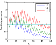
Figure 1: The $x$-axis is $K$. The $y$-axis gives the average influence parameter $I(K)$. We show the cases where $\rho=1/5,1/6,1/7$. For larger $\rho$ we reach quiescent behavior more rapidly with increasing $K$.

We show that for $d$ large enough, $I(d)$ tends to 0. For convenience, assume that $d$ is an even integer and $\theta d$ is non-integral. By tail bounds on binomial coefficients, $2^{-d}\sum_{r\geq\lfloor d/2+\rho d\rfloor}\binom{d}{r}<2^{-cd}$ for some constant $c$. (This can be proven using a Chernoff bound, such as Theorem 4.1 in Motwani and Raghavan (1995).) Hence ${I}(d)<1$ for large enough $d$, and tends to zero as $d$ increases. We had previously noted that it is commonly assumed that $I(d)$ is linear in $d$. Strong majority transfer functions feature $I(d)$ that is clearly non-linear, and we therefore expect this assumption to be consequential. To illustrate, consider two network structures: one with a fixed $K=4$, and another where the indegree distribution follows a power law with mean $K=4$. Using $\theta=1/3$, in the former, we get ${\cal I}=I(K)=1.5$, while in the latter (with $K_{max}=100$), ${\cal I}=0.79$. Thus, while a fixed $K$ yields decidedly chaotic dynamics, using a power law distribution with the same mean indegree produces quiescence.

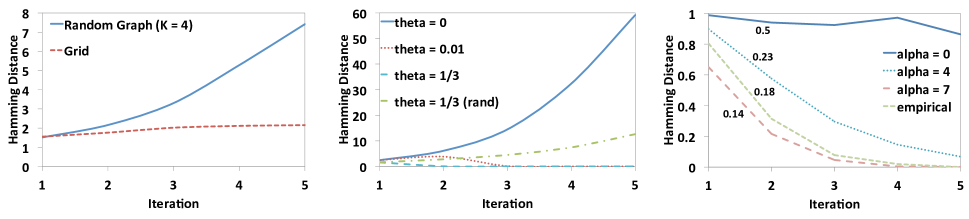
Figure 2: Boolean network dynamics (Hamming distance over time, starting with single-bit perturbations). Left: comparing random graph with $K=4$ and a grid. Middle: random networks with fixed $K=10$ and unbalanced strong majorities. Right: random networks with $K=5$, using nested canalizing functions, with degree of imbalance increasing with $\alpha$, and the empirical distribution of 5-input transfer functions based on yeast regulatory networks Kauffman et al. (2003); Harris et al. (2002).

The importance of graph structure. Our results rely fundamentally on the fact that the inputs into each node are chosen independently. The fact that the size of the neighborhood at distance $t$ grows exponentially with $t$ is crucial for our proofs. Furthermore (for the random graphs we sample from), this neighborhood is a root directed tree, when $t<t^{*}$. When graphs exhibit only polynomial local growth, we do not expect chaotic dynamic behavior even when other conditions for it are met. We illustrate this point in Figure 2 (left), which compares a random network with $K=4$ to a grid (a bidirectional square lattice that also has $K=4$). While both initially appear to be in a chaotic regime, the Hamming distance stops diverging for a grid, but diverges exponentially in the random network.

The importance of being balanced. The assumption that ${\cal T}$ is balanced is crucial. Balance has previously been noted to play an important role in determining the order to chaos transition, but entirely under the assumption that each truth table entry is i.i.d. Kauffman (1993). It has been pointed out that much of the resulting space of parameter values gives rise to chaotic dynamics Aldana and Cluzel (2003). What we now demonstrate is that this observation is largely an artifact of independence, and when truth table entries are not independently distributed, even a slight deviation from balance (homogeneity) may push Boolean network dynamics to quiescence. Consider networks in which every transfer function is a strong majority (with $\theta=0$ being a simple majority). We get a balanced distribution of transfer function by choosing between $\theta$ and $-\theta$ with equal probability. An imbalanced distribution is obtained by choosing only one of them. Figure 2 (middle) shows several examples of how the Hamming distance evolves for different values of $\theta$, and contrasts the balanced and unbalanced settings. The difference could hardly be more dramatic: even a slight deviation from simple majority ($\theta=0.01$) is a difference between chaos and quiescence; indeed, it is instructive to see the initial increase in Hamming distance for the imbalanced strong majority with $\theta=0.01$, only to be ultimately suppressed. Similarly, we can compare the balanced and unbalanced versions of strong majorities with $\theta=1/3$: the balanced version is clearly chaotic, while in the network with the unbalanced analogue, initial perturbation effects erode within two iterations. A similar picture emerges when we consider nested canalizing functions, previously offered as an explanation of robustness in genetic regulatory networks Harris et al. (2002); Kauffman et al. (2003). Classes of these are generated by a parameter $\alpha$ that governs the fraction of 1’s in the transfer function truth table, with larger values of $\alpha$ leading to greater imbalance. Figure 2 (right) compares evolution of networks with nested canalizing functions, as well as with transfer functions following an empirical distribution of transfer functions based on regulatory networks Kauffman et al. (2003). We see that the main driver of quiescence appears to be the internal inhomogeneity of transfer functions, rather than canalizing properties.

Sandia is a multiprogram laboratory operated by Sandia Corporation, a wholly owned subsidiary of Lockheed Martin Corporation, for the U.S. Department of Energy under contract DE-AC04-94AL85000.

Supplemental Material

The following supplemental material for the paper includes all formalization and proof details.

Appendix A Preliminaries and notation

We will be using probabilities very heavily, so it will help to set some notations. Capital letters $X,Y,Z$ will used to denote random variables. Events are denoted by calligraphic letters ${\cal E},{\cal F},\ldots$. The probability of an event ${\cal E}$ is denoted by ${\rm Pr}({\cal E})$. The expectation of a random variable $X$ is denoted by $\hbox{\bf E}[X]$. The random variable $X$ conditioned on event ${\cal E}$ is denoted by $X|{\cal E}$.

A.1 Preliminaries

Graphs: We will always deal with directed graphs $G=(V,E)$. The set $V$ will be $[n]$, the set of positive integers upto $n$. For every $i\in V$, $N^{+}(i)$ (resp. $N^{-}(i)$) denotes the set of out (resp. in) neighbors of $i$ in $G$. We use $d^{+}(i)$ to denote the outdegree of $i$ (similarly, define $d^{-}(i)$).

Boolean strings and functions: We will use the set $\{-1,+1\}$ (instead of $\{0,1\}$) to denote bits, thereby aligning ourselves with the theory of Boolean functions. The $n$-dimensional Boolean hypercube is denoted by ${\cal B}^{n}=\{-1,+1\}^{n}$. This is also a representation for all $n$ bit strings. A Boolean function is a function $f:{\cal B}^{n}\rightarrow{\cal B}^{1}$.

For any two elements $x,y\in{\cal B}_{n}$, $\Delta(x,y)$ is the Hamming distance between $x$ and $y$. For $x\in{\cal B}^{n}$, $x^{(i)}$ is the unique element of ${\cal B}^{n}$ which is the same as $x$ on all coordinates except for the $i$th coordinate. We use $x_{i}$ to denote the $i$th coordinate of $x$.

We use ${\rm Pr}_{x}({\cal E})$ (where ${\cal E}$ is some event) to denote the probability of ${\cal E}$ over the uniform distribution of $x$ (which means we choose an $x$ uniformly at random from ${\cal B}^{n}$ and check the probability of ${\cal E}$). Similarly, $\hbox{\bf E}_{x}[\ldots]$ denotes the expectation over a random uniform $x$.

Boolean networks: A Boolean network ${\cal N}$ consists of a directed graph $G$ and a set of transfer functions $T$. The set $T$ has a transfer function $\tau_{v}:{\cal B}^{d^{-}(i)}\longrightarrow\{-1,+1\}$, for each $i\in V$.

The state of a Boolean network is just an assignment of $\{-1,+1\}$ to each vertex in $V$. This can be represented as an $n$-bit string, or alternately, an element $x$ of the $n$-dimensional Boolean hypercube ${\cal B}^{n}=\{-1,+1\}^{n}$.

Suppose ${\cal N}$ starts at the state $x$. The state at vertex $i$ after $t$ steps of ${\cal N}$ is denoted by the Boolean function $f_{t,i}(x)$. The function $f_{t}(x):{\cal B}^{n}\rightarrow{\cal B}^{n}$ is state of ${\cal N}$ after $t$-steps (so this is an $n$-dimensional vector having $f_{t,i}(x)$ as its $i$th coordinate).

Assumptions on Boolean network: We will analyze Boolean networks that arise from a particular distribution. First, the graph $G$ is chosen from a random distribution. We will assume some fixed indegree distribution ${\cal D}$. (This is simply a distribution on positive integers.) For each vertex $i$, we independently choose $d^{-}(i)$ from ${\cal D}$. Then, we choose $d^{-}(i)$ uniform random vertices (without replacement) to be the in-neighborhood ($N^{-}(i)$) of $i$. We denote the average indegree by $K$, and the maximum possible indegree by $K_{max}$.

Next, we assume that there is a distribution ${\cal T}$ on transfer functions. Formally, this is a union of distributions ${\cal T}_{d}$, where this family only contains Boolean functions that take $d$ inputs. For each vertex $i$, we first choose an independent function $\tau_{i}(x_{1},x_{2},\ldots,x_{d^{-}(i)})$ from ${\cal T}_{d^{-}(i)}$. Sort $N^{-}(i)$ (according to its label) to get $v_{1},v_{2},\ldots,v_{d^{-}(i)}$. Assign the vertex $v_{j}$ to input $x_{j}$ of $\tau_{i}$. This gives us the transfer function for vertex $i$.

We will assume that the family ${\cal T}$ has either of the following properties:

• Full independence: A random function in ${\cal T}$ is generated by taking an empty truth table, and filling in each entry independently with the same distribution.

• Balance on average: A uniform random member of ${\cal T}$ evaluated on a uniform random input outputs $+1$ with probability $1/2$. Formally, ${\rm Pr}_{x,\tau}[\tau(x)=+1]$ $=1/2$ $={\rm Pr}_{x,\tau}[\tau(x)=-1]$

A.2 Influences

We now discuss some of our main definitions. The following is one of the most important concepts.

Definition 3

For a Boolean function $f$ and coordinate $i$, the influence of $i$ on $f$, denoted by ${\rm{Inf}}_{i}(f)$ is ${\rm Pr}_{x}[f(x)\neq f(x^{(i)})]$. The total influence of $f$ is $\sum_{i}{\rm{Inf}}_{i}(f)$ and the average influence of $f$ is $\frac{1}{n}\sum_{i}{\rm{Inf}}_{i}(f)$.

For a distribution ${\cal T}=\cup_{d}{\cal T}_{d}$ of transfer functions, the influence of the distribution ${\cal T}_{d}$ is denoted by ${I}({\cal T}_{d})$. Formally, ${I}({\cal T}_{d})=\hbox{\bf E}_{\tau}[\sum_{i}{\rm{Inf}}_{i}(\tau)]$. Often, when the defintion of ${\cal T}$ is unambiguous, we write this as ${I}_{d}$.

Definition 4

The influence of $i$ at time $t$ on ${\cal N}$, denoted by ${\rm{Inf}}_{t,i}({\cal N})$, is $\hbox{\bf E}_{x}[\Delta(f_{t}(x),f_{t}(x^{(i)}))]$. The average influence at time $t$ is $\frac{1}{n}\sum_{i}{\rm{Inf}}_{t,i}({\cal N})$.

Claim 5

The average influence of ${\cal N}$ at time $t$ can be expressed as $\frac{1}{n}\sum_{1\leq i,j\leq n}{\rm{Inf}}_{i}(f_{t,j})$.

Proof: Let us focus on ${\rm{Inf}}_{i}({\cal N})$. We choose a uniform random $x$ and evolve ${\cal N}$ from the states $x$ and $x^{(i)}$. Let $\chi(t,j)$ be the indicator random variable for the event that $f_{t,j}(x)\neq f_{t,j}(x^{(i)})$. Note that $\hbox{\bf E}_{x}[\chi(t,j)]={\rm{Inf}}_{i}(f_{t,j})$. By the definition of Hamming distance and linearity of expectation,

$${\rm{Inf}}_{i}({\cal N}) = \hbox{\bf E}_{x}[\Delta(f(x),f(x^{(i)}))]$$

$$= \hbox{\bf E}_{x}[\sum_{j}\chi(t,j)]=\sum_{j}\hbox{\bf E}_{x}[\chi(t,j)]=\sum_{j}{\rm{Inf}}_{i}(f_{t,j})$$

Averaging this equality over all $i$ completes the proof. $\Box$

We will need the following simple facts about influences. (This is a restatement of Proposition 2.

Proposition 6

• Consider a function $f:{\cal B}^{d}\rightarrow{\cal B}$. An edge of the Boolean hypercube ${\cal B}^{d}$ is called bichromatic if one endpoint is labelled $+1$ and the other is labelled $-1$. Then $\sum_{i\leq d}{\rm{Inf}}_{i}(f)=$ $(\textrm{\# bichromatic edges})/2^{d-1}$.

  Consider a distribution ${\cal T}$ over functions $f:{\cal B}^{d}\rightarrow{\cal B}$.

  $$\hbox{\bf E}[\sum_{i\leq d}{\rm{Inf}}_{i}(f)]=(1/2^{d-1})\sum_{e:\textrm{edge}\ \in{\cal B}^{d}}\Pr[\textrm{$e$ is bichromatic}]$$

• For any Boolean function $f$ and input index $i$,

  $$\Pr_{x}[(f(x)=1)\wedge(f(x)\neq f(x^{(i)}))]$$

  $$= \Pr_{x}[(f(x)=-1)\wedge(f(x)\neq f(x^{(i)}))]={\rm{Inf}}_{i}(f)/2$$

Proof: Consider all pairs $(y,y^{(i)})$, where the $i$th bit of $y$ is $1$. These pairs form a partition of the hypercube and are actually all edges of the hypercube parallel to the $i$th dimension. The influence ${\rm{Inf}}_{i}(f)$ is exactly the probability that a uniformly random $x$ belongs to a bichromatic pair. Let $B_{i}$ be the number of bichromatic pairs. Noting that the total number of edges parallel to the $i$th dimension is $2^{d-1}$, ${\rm{Inf}}_{i}(f)=B_{i}/2^{d-1}$. Summing over all $i$, we get that $\sum_{i\leq d}{\rm{Inf}}_{i}(f)=$ $(\textrm{\# bichromatic edges})/2^{d-1}$. To deal with a distribution, we simply apply linear of expectation to this bound.

Now for the second part. When does the event $(f(x)=1)\wedge(f(x)\neq f(x^{(i)}))$ happen? This happens when $x$ belongs to a bichromatic pair, and $f(x)=1$. Exactly half the member of bichromatic pairs have value $1$ (or $-1$). Hence, $\Pr_{x}[(f(x)=1)\wedge(f(x)\neq f(x^{(i)}))]={\rm{Inf}}_{i}(f)/2$.

We restate Theorem 1 for convenience.

Theorem 1

The average influence at time $t\leq t^{*}$ for the Boolean network ${\cal N}$ lies in the range $(\sum_{d\geq 1}p_{d}{I}_{d})^{t}\pm 1/n^{1/4}$.

Appendix B Proof strategy

Before diving into the gory details of the proof of our main result, we offer a high level intuition of the overall proof. The proof essentially consists of two central steps, Lemma 9 and Claim 11, discussed in Sections C and D respectively. Lemma 9 considers an idealized situation where the underlying graph of a Boolean network is simply a root-directed tree. Any modification of the state of a leaf travels up the tree, possibly affecting the root. In this case, we can give an exact expression of the influence of leaves on the root. Our key next step is Claim 11, which proves that for our distribution of graph topologies (which is closely related to the configuration model), the logarithmic-distance neighborhood of most nodes looks like a root-directed tree. Note that this does not imply that the graph itself decomposes into disjoint tree, since the trees rooted at each node are interconnected in complicated ways.

These two steps are combined together for the final proof in Section E. This proof makes heavy use of the linearity of expectation and some conditional probability arguments. It enables us to perform exact short-run analysis of the Boolean network by only considering local neighborhoods of an “average” node.

At the core of the proof of Lemma 9 is a straightforward induction argument. Consider a tree network, where we change the state at some leaf. The catch is that induction requires the family of transfer functions to satisfy the technical conditions of balance or full independence. This is one of the major insights of this work, since these conditions on transfer function families have generally been implicit in previous results. The proof forces us to make these conditions explicit. Section C has the details.

The proof of Claim 11 consists of a combinatorial probability calculation. We are generating our graph through the randomized process of choosing the (immediate) neighborhood for each node independently (and uniformly) at random. We show that the probability that the short-distance neighborhood of a node contains a cycle is extremely small. The formal proof is given in Section D.

Appendix C Influences on trees

In this section, we will make some arguments about tree networks. Let $T$ be a directed tree (so all edges point towards the root) with all leaves at the same depth $h$. We are interested in the influence of the leaf variables on the root $r$. Let the function giving the state of the root $r$ at time $t$ be $f_{t,r}$. Note that $f_{h,r}$ is only a function of the leaves, since there is no feedback in this graph. Note that we are not particularly bothered with what happens in the leaves are time step $1$ (since those values are not even defined). We are merely interested in how the values at the leaves will propagate up the tree. For each $v$, the transfer function $\tau_{v}$ is chosen from ${\cal T}$ (technically, from ${\cal T}_{d^{-}(v)}$).

Claim 7

Let $T$ be a tree of depth $h$. For a leaf $\ell$, let the path to the root be $v_{0}=\ell,v_{1},v_{2},\ldots,v_{h}=r$. Then, $\hbox{\bf E}_{\cal T}[{\rm{Inf}}_{\ell}(f_{h,r})]=\prod_{i=1}^{h}\hbox{\bf E}_{{\cal T}}[{\rm{Inf}}_{v_{i-1}}(\tau_{v_{i}})]$. (We remind the reader that ${\cal T}$ is either balanced on average or fully independent.)

Proof: We prove by induction on the depth $h$. When ${\cal T}$ is balanced on average, we will also show that $\hbox{\bf E}_{{\cal T},x}[f_{h,r}(x)=1]=1/2$. For the base case, set $h=1$. Hence, all the leaves are directly connected to the root, and the set ${\cal T}$ has only one function $\tau_{r}$ (for the root $r$). The probability (over $x$) that $\tau_{r}(x)=\tau_{r}(x^{(\ell)})$ is exactly ${\rm{Inf}}_{\ell}(\tau_{r})$. Suppose ${\cal T}$ is balanced on average. Since $f_{1,r}=\tau_{r}$, ${\rm Pr}_{{\cal T},x}[f_{1,r}(x)=1]={\rm Pr}_{{\cal T},x}[\tau_{r}(x)=1]=1/2$.

Now for the induction step. Assume the claim is true for trees of depth $h-1$. We will denote the indegree of $r$ by $d$. The root $r$ is connected to a series of subtrees $T_{1},T_{2},\ldots,T_{d}$ of depth $h-1$. The roots of each of these $r_{1},r_{2},\ldots,r_{d}$ are the children of $r$. For convenience, assume that $\ell\in T_{1}$. Note that for $b\neq 1$ and $\forall x$, $f_{h-1,r_{b}}(x)=f_{h-1,r_{b}}(x^{(\ell)})$. In the final step, the function evaluated is $\tau_{r}(f_{h-1,r_{1}}(x),f_{h-1,r_{2}}(x),\ldots,f_{h-1,r_{d}}(x))$.

First, let us assume that ${\cal T}$ is fully independent (the proof is much easier in this case). The probability that $f_{h-1,r_{1}}(x)\neq f_{h-1,r_{1}}(x^{(\ell)})$ is, by the induction hypothesis, $\prod_{i=1}^{h-1}\hbox{\bf E}_{{\cal T}}[{\rm{Inf}}_{v_{i-1}}(\tau_{v_{i}})]$. Conditioned on this, what is the probability that $\tau_{v}(f_{h-1,r_{1}}(x),\ldots,)$ $\neq\tau_{v}(f_{h-1,r_{1}}(x^{(\ell)}),\ldots)$? Since each entry in the truth table of $\tau_{v}$ is chosen independently, this probability is exactly $\hbox{\bf E}_{{\cal T}}[{\rm{Inf}}_{v_{h-1}}(\tau_{v_{h}})]$. Multiplying, we get that $\hbox{\bf E}_{\cal T}[{\rm{Inf}}_{\ell}(f_{h,r})]=\prod_{i=1}^{h}\hbox{\bf E}_{{\cal T}}[{\rm{Inf}}_{v_{i-1}}(\tau_{v_{i}})]$. This completes the proof for this case.

Now, we assume that ${\cal T}$ is balanced on average. For convenience, set random variable $X_{i}=f_{h-1,r_{i}}(x)$, and $X^{\prime}_{1}$ to be $f_{h-1,r_{1}}(x^{(\ell)})$. For a bit $b$, let ${\cal E}_{i}(b)$ denote the event that $X_{i}=b$. We set ${\cal F}$ to denote the event that $X_{1}\neq X^{\prime}_{1}$. We use $\bar{b}$ as shorthand for a vector $b_{1},\ldots,b_{d}$ of bits. The indicator $\chi(\bar{b})$ is $1$ when $\tau_{v}(\bar{b})\neq\tau_{v}(\bar{b}^{(1)})$.

$$\hbox{\bf E}_{\cal T}[{\rm{Inf}}_{\ell}(f_{h,r})]$$

$$= \hbox{\bf E}_{\cal T}[\Pr_{x}[\tau_{v}(f_{h-1,r_{1}}(x),f_{h-1,r_{2}}(x),\ldots,f_{h-1,r_{d}}(x))$$

$$\neq\tau_{v}(f_{h-1,r_{1}}(x^{(\ell)}),f_{h-1,r_{2}}(x^{(\ell)}),\ldots,f_{h-1,r_{d}}(x))]]$$

$$= \hbox{\bf E}_{\cal T}[\Pr_{x}[\tau_{v}(X_{1},X_{2},\ldots,X_{d})\neq\tau_{v}(X^{\prime}_{1},X_{2},\ldots,X_{d})]]$$

$$= \hbox{\bf E}_{\cal T}[\sum_{\bar{b}}\chi(\bar{b})\Pr_{x}[\bigwedge_{i}{\cal E}_{i}(b_{i})\wedge{\cal F}]]$$

$$= \hbox{\bf E}_{\cal T}[\sum_{\bar{b}}\chi(\bar{b})\Pr_{x}[{\cal E}_{1}(b_{1})\wedge{\cal F}]\Pr_{x}[\prod_{i=2}^{d}{\cal E}_{i}(b_{i})]]$$

$$= \sum_{\bar{b}}\hbox{\bf E}_{\cal T}[\chi(\bar{b})\Pr_{x}[{\cal E}_{1}(b_{1})\wedge{\cal F}]\Pr_{x}[\prod_{i=2}^{d}{\cal E}_{i}(b_{i})]]$$

$$= \sum_{\bar{b}}\hbox{\bf E}_{\cal T}[\chi(\bar{b})\Pr_{x}[{\cal E}_{1}(b_{1})\wedge{\cal F}]]\Pr_{x}[\prod_{i=2}^{d}\hbox{\bf E}_{\cal T}[{\cal E}_{i}(b_{i})]]$$

$$= \sum_{\bar{b}}\hbox{\bf E}_{\cal T}[\chi(\bar{b})\Pr_{x}[{\cal E}_{1}(b_{1})\wedge{\cal F}]]\prod_{i=2}^{d}\hbox{\bf E}_{\cal T}[\Pr_{x}[f_{h-1,r_{i}}=b_{i}]]$$

$$= (1/2)^{d-1}\sum_{\bar{b}}\hbox{\bf E}_{\cal T}[\chi(\bar{b})\Pr_{x}[{\cal E}_{1}(b_{1})\wedge{\cal F}]]$$

The final step uses the induction hypothesis. Now, we use Proposition 2 to deal with $\Pr_{x}[{\cal E}_{1}(b_{1})\wedge{\cal F}]]$ $=\Pr_{x}[f_{h-1,r_{1}}(x)\neq b_{1}\wedge(f_{h-1,r_{1}}(x)=f_{h-1,r_{1}}(x^{(\ell)}))]$. Let ${\cal T}^{\prime}$ be the distribution of transfer functions excluding $\tau_{r}$.

$$\hbox{\bf E}_{\cal T}[{\rm{Inf}}_{\ell}(f_{h,r})] = (1/2)^{d-1}\sum_{\bar{b}}\hbox{\bf E}_{\cal T}[\chi(\bar{b})\Pr_{x}[{\cal E}_{1}(b_{1})\wedge{\cal F}]]$$

$$= (1/2)^{d}\sum_{\bar{b}}\hbox{\bf E}_{\cal T}[\chi(\bar{b}){\rm{Inf}}_{\ell}(f_{h-1,r_{1}})]$$

$$= \hbox{\bf E}_{{\cal T}^{\prime}}[{\rm{Inf}}_{\ell}(f_{h-1,r_{1}})](1/2)^{d}\sum_{\bar{b}}\hbox{\bf E}_{{\cal T}_{r}}[\chi(\bar{b})]$$

$$= \prod_{i=1}^{h-1}\hbox{\bf E}_{{\cal T}}[{\rm{Inf}}_{v_{i-1}}(\tau_{v_{i}})]\hbox{\bf E}_{{\cal T}}[\Pr_{\bar{b}}[\chi(\bar{b})]]$$

$$= \prod_{i=1}^{h-1}\hbox{\bf E}_{{\cal T}}[{\rm{Inf}}_{v_{i-1}}(\tau_{v_{i}})]\hbox{\bf E}_{{\cal T}}[{\rm{Inf}}_{1}(\tau_{r})]$$

$$= \prod_{i=1}^{h}\hbox{\bf E}_{{\cal T}}[{\rm{Inf}}_{v_{i-1}}(\tau_{v_{i}})]$$

$\Box$

Consider a tree $T$ where all leaves have fixed depth $h$. Set $L$ to be the set of all leaves of $T$. Define ${\rm{Inf}}(T)=\sum_{\ell\in L}{\rm{Inf}}_{\ell}(f_{h,r})$. For a leaf $\ell$ that is a descendant of some vertex $v$, suppose the path between them is $v_{0}=\ell,v_{1},v_{2},\ldots,v_{a}=v$. Define ${\rm{Infprod}}_{\ell,v}=\prod_{i=1}^{a}{\rm{Inf}}_{v_{i-1}}(\tau_{v_{i}})$.

Lemma 8

Let $r_{1},r_{2},\ldots,r_{a}$ be the children of the root $r$. Let $T_{i}$ be the subtree rooted at $r_{i}$. Then, $\hbox{\bf E}_{\cal T}[{\rm{Inf}}(T)]=\sum_{i}\hbox{\bf E}_{{\cal T}_{r}}[{\rm{Inf}}_{r_{i}}(\tau_{r})]\hbox{\bf E}_{\cal T}[{\rm{Inf}}(T_{i})]$.

Proof: Define $L_{i}$ to be the set of leaves of $T_{i}$.

$$\hbox{\bf E}_{\cal T}[{\rm{Inf}}(T)] = \hbox{\bf E}_{\cal T}[\sum_{\ell\in L}{\rm{Inf}}_{\ell}(f_{h,r})]$$

$$= \sum_{i}\hbox{\bf E}_{\cal T}[\sum_{\ell\in L_{i}}{\rm{Inf}}_{\ell}(f_{h,r})]$$

$$= \sum_{i}\sum_{\ell\in L_{i}}\hbox{\bf E}_{\cal T}[{\rm{Infprod}}_{\ell,r}]$$

$$= \sum_{i}\sum_{\ell\in L_{i}}\hbox{\bf E}_{{\cal T}_{r}}[{\rm{Inf}}_{r_{i}}(\tau_{r})]\hbox{\bf E}_{\cal T}[{\rm{Infprod}}_{\ell,r_{i}}]$$

$$= \sum_{i}\hbox{\bf E}_{{\cal T}_{r}}[{\rm{Inf}}_{r_{i}}(\tau_{r})]\sum_{\ell\in L_{i}}\hbox{\bf E}_{\cal T}[{\rm{Infprod}}_{\ell,r_{i}}]$$

$$= \sum_{i}\hbox{\bf E}_{{\cal T}_{r}}[{\rm{Inf}}_{r_{i}}(\tau_{r})]\hbox{\bf E}_{\cal T}[{\rm{Inf}}(T_{i})]$$

$\Box$

Consider the following randomized tree construction. First, we have a probability $p_{d}$, for all positive integers $d$. We define this construction recursively. Trees of height $0$ are just singleton vertices. To construct a tree of height $h\geq 1$, we first have a root $r$. We choose the number of children to be $d$ with probability $p_{d}$. Then, for each child, we recursively construct a tree of height $h-1$.

Lemma 9

Consider a completely balanced tree $T$ with root $r$ and height $h$ generated by the randomized procedure described above. Furthermore, let the transfer functions be chosen as described above. Then $\hbox{\bf E}[\sum_{\ell\in T}{\rm{Inf}}_{\ell}(f_{h,r})]=$ $(\sum_{d\geq 1}p_{d}{I}_{d})^{h}$.

Proof: For any vertex $v$, let $T_{v}$ be the subtree rooted at $v$. We will show by induction on $h$, that for any vertex at height $h$, $\hbox{\bf E}[\sum_{\ell\in T_{v}}{\rm{Inf}}_{\ell}(f_{h,v})]=$ $(\sum_{d\geq 1}p_{d}{I}_{d})^{h}$.

For vertex $v$ with $h=0$, we trivially have ${\rm{Inf}}_{v}(f_{0,v})=1$. Now consider $v$ at some height $h$. Suppose $v$ has $d$ children $v_{1},\ldots,v_{d}$. For each child $v_{i}$ of $v$, $\hbox{\bf E}_{{\cal T}_{v}}{\rm{Inf}}_{v_{i}}(\tau_{v})=I_{d}$. By the induction hypothesis, $\hbox{\bf E}[{\rm{Inf}}(T_{v_{i}})]$ (which are identical for all $i$) has value exactly $(\sum_{d\geq 1}p_{d}{I}_{d})^{h-1}$. By Lemma 8, conditioned on $v$ having $d$ children $\hbox{\bf E}[\sum_{\ell\in T_{v}}{\rm{Inf}}_{\ell}(f_{h,v})]$ $=\sum_{i\leq d}\hbox{\bf E}_{{\cal T}_{r}}[{\rm{Inf}}_{v_{i}}(\tau_{v})]\hbox{\bf E}[{\rm{Inf}}(T_{v_{i}})]=$ $I_{d}(\sum_{d\geq 1}p_{d}{I}_{d})^{h-1}$. By noting that the probability that $v$ has $d$ children is $p_{d}$, $\hbox{\bf E}[\sum_{\ell\in T_{v}}{\rm{Inf}}_{\ell}(f_{h,v})]=$ $(\sum_{d\geq 1}p_{d}{I}_{d})^{h}$. $\Box$

Appendix D The topology of the Kauffman network

We now prove some topological properties of the random graphs (which are effectively directed Erdős-Rényi graphs). We remind that reader that the indegrees for all vertices are chosen independently from the same distribution.

Definition 10

The distance $t$ in-neighborhood of $i$ is denoted by $N^{-}_{t,i}$. This is the set of all vertices whose shortest path distance (along directed paths) to $i$ is exactly $t$. We set $N^{-}_{\leq t,i}=\bigcup_{s\leq t}N^{-}_{s,i}$.

We define $t^{*}=\log n/(4\log K_{max})$.

Claim 11

Fix a vertex $i$ and let $t\leq t^{*}$. Let ${\cal E}_{i}$ denote the event that the subgraph induced by $N^{-}_{\leq t^{*},i}$ is a directed tree with edges directed towards root $i$. Then, $|N^{-}_{\leq t^{*},i}|\leq n^{1/4}$ and ${\rm Pr}({\cal E}_{i})\geq 1-1/\sqrt{n}$.

Proof: Let us start with an empty graph, and slowly add random edges in a prescribed order. We begin with $i$, and then choose the incoming edges. This gives the set $N^{-}_{1,i}$. Then, we choose all the in-neighbors of $N^{-}_{1,i}$. This is done by iterating over all vertices in $N^{-}_{1,i}$, and for each such vertex, selecting every vertex as a neighbor with probability $K/n$. This gives us $N^{-}_{2,i}$. Proceeding this way, we incrementally build up $N^{-}_{\leq t^{*},i}$. Note that $|N^{-}_{\leq t^{*},i}|\leq K_{max}^{t^{*}}=n^{1/4}$.

Consider the construction of $N^{-}_{\leq t,i}$. Every new element added to this set is a uniform random element from $[n]$. Consider a random sequence of $n^{1/4}$ elements chosen uniformly at random (with replacement) from $[n]$. The probability that no element is repeated at least

$$\left(1-\frac{n^{1/4}}{n}\right)^{n^{1/4}}\geq\exp(-\sqrt{n}/n)\geq 1-(\sqrt{n})^{-1}$$

If no element in $N^{-}_{\leq t,i}$ is repeated, then the subgraph induced by $N^{-}_{\leq t,i}$ is a directed tree. $\Box$

Appendix E Proof of the Main Theorem

We are now ready to prove our main result.

Proof: (of Theorem 1) By Claim 5, the average influence at time $t$ is $(\sum_{i}\sum_{j}{\rm{Inf}}_{j}(f_{t,i}))/n$. For a fixed vertex $i$, let us compute $\sum_{j}{\rm{Inf}}_{j}(f_{t,i})$. Denote this quantity by $X$. We apply Bayes rule to split $\hbox{\bf E}[X]$ into conditional expectations.

$$\hbox{\bf E}[X]={\rm Pr}({\cal E}_{i})\hbox{\bf E}[X|{\cal E}_{i}]+{\rm Pr}(\overline{{\cal E}_{i}})\hbox{\bf E}[X|\overline{{\cal E}_{i}}]$$

Observing that $X$ is always positive and applying Claim 11, we get $\hbox{\bf E}[X]\geq(1-1/\sqrt{n})\hbox{\bf E}[X|{\cal E}_{i}]$. Note that since ${\rm{Inf}}_{j}(f_{t,i})\leq 1$, $X\leq|N^{-}_{t,i}|\leq n^{1/4}$. Hence $\hbox{\bf E}[X]\geq\hbox{\bf E}[X|{\cal E}_{i}]-n^{-1/4}$. We now obtain an upper bound applying Claim 11 again.

$$\hbox{\bf E}[X] \leq {\rm Pr}({\cal E}_{i})\hbox{\bf E}[X|{\cal E}_{i}]+(1/\sqrt{n})\hbox{\bf E}[X|\overline{{\cal E}_{i}}]$$

$$\leq \hbox{\bf E}[X|{\cal E}_{i}]+n^{-1/4}$$

It only remains to determine $\hbox{\bf E}[X|{\cal E}_{i}]$. Conditioned on ${\cal E}_{i}$, the induced subgraph on $N^{-}_{\leq t,i}$ is a directed tree. We apply Lemma 9 to complete the proof. $\Box$

References

- Kauffman (1969) S. A. Kauffman, Journal of Theoretical Biology 22, 437 (1969).
- Kauffman (1993) S. A. Kauffman, Origins of Order (Oxford University Press, 1993).
- Harris et al. (2002) S. E. Harris, B. K. Sawhill, A. Wuensche, and S. A. Kauffman, Complexity 7, 23 (2002).
- Shmulevich and Kauffman (2004) I. Shmulevich and S. A. Kauffman, Physical Review Letters 93, 048701 (2004).
- Moreira and Amaral (2005) A. A. Moreira and L. A. N. Amaral, Physical Review Letters 94, 218702 (2005).
- Aldana and Cluzel (2003) M. Aldana and P. Cluzel, Proceedings of the National Academy of Sciences 100, 8710 (2003).
- Kauffman et al. (2003) S. A. Kauffman, C. Peterson, B. Samuelsson, and C. Troein, Proceedings of the National Academy of Sciences 100, 14796 (2003).
- Shmulevich et al. (2003) I. Shmulevich, H. Lahdesmaki, E. R. Dougherty, J. Astola, and W. Zhang, Proceedings of the National Academy of Sciences 100, 10734 (2003).
- Derrida and Pomeau (1986) B. Derrida and Y. Pomeau, Europhysics Letters 1, 45 (1986).
- (10) F. Ghanbarnejad and K. Klemm, “Stability of Boolean and continuous dynamics,” http://arxiv.org/abs/1103.4490v2.
- Kahn et al. (1988) J. Kahn, G. Kalai, and N. Linial, in Twenty-Ninth Symposium on the Foundations of Computer Science (1988) pp. 68–80.
- Greil and Drossel (2007) F. Greil and B. Drossel, European Physical Journal B 57, 109 (2007).
- Szejka et al. (2008) A. Szejka, T. Mihalijev, and B. Drossel, New Journal of Physics 10 (2008).
- Raeymaekers (2002) L. Raeymaekers, Journal of Theoretical Biology 218, 331 (2002).
- Motwani and Raghavan (1995) R. Motwani and P. Raghavan, Randomized Algorithms (Cambridge University Press, 1995).