Adaptive-optics assisted near-infrared polarization measurements of sources in the Galactic Center

Abstract

Context. The Galactic Center offers unique opportunities to study stellar and bow-shock polarization effects in a dusty environment.

Aims. The goals of this work are to provide near-infrared (NIR) polarimetry of the stellar sources in the central parsec at the resolution of an 8m telescope for the first time, along with new insights into the nature of the known bright bow-shock sources.

Methods. We use adaptive-optics assisted observations obtained at the ESO VLT in the H- and Ks-band, applying both high-precision photometric methods specifically developed for crowded fields and a newly established polarimetric calibration for NACO to produce polarization maps of the central 3”$\times$19”, in addition to spatially resolved polarimetry and a flux variability analysis on the extended sources in this region.

Results. We find foreground polarization mainly parallel to the Galactic plane, with average values of (4.6 $\pm$ 0.6)% at $26^{\circ}\pm 6^{\circ}$ (Ks-band) and (9.3 $\pm$ 1.3)% at $20^{\circ}\pm 6^{\circ}$ (H-band) in the center of the field-of-view (FOV). Further away from the center, we find higher polarization degrees and steeper polarization angles: (7.5 $\pm$ 1.0)% at $11^{\circ}\pm 6^{\circ}$ (Ks-band) and (12.1 $\pm$ 2.1)% at $13^{\circ}\pm 6^{\circ}$ (H-band). $p_{H}/p_{Ks}$ peaks at $1.9\pm 0.4$, corresponding to a power law index for the wavelength dependency of $\alpha=2.4\pm 0.7$. These values also vary over the FOV, with higher values in the center. This is indicative of the influence of local effects on the total polarization, possibly dichroic extinction by Northern Arm dust. The two extended sources IRS 21 and 1W show similar intrinsic polarization degrees of 6.1 resp. 7.8% (Ks) and 6.9 (H, only 1W) at polarization angles coincident with previous NIR and mid-infrared (MIR) findings, both in total and spatially resolved. The spatial polarization pattern of both sources points to scattering on aligned elongated dust grains as the major source of intrinsic polarization, and matches the known orientation of the magnetic field. Our data also allow us to separate the bow shock of IRS 21 from the central source for the first time in the Ks-band, finding the apex north of the central source and determining a standoff distance of $\sim$400 AU, which matches previous estimates. This source also shows a $\sim 50$% increase in flux in the NIR over several years.

1 Introduction

The center of the Milky Way is located at a distance of $\sim 8.0$ kpc (Ghez et al., 2008; Gillessen et al., 2009). It contains a nuclear stellar cluster (NSC) with a $\sim 4.0\times 10^{6}$ M_☉ super-massive black hole at its dynamical center (Eckart et al., 2002; Schödel et al., 2002, 2003; Ghez et al., 2003, 2008; Gillessen et al., 2009). This cluster shows similar properties as the NSCs found at the dynamical and photometric centers of other galaxies (Böker, 2010; Schödel, 2010c).
Less than a decade after the first near-infrared (NIR) imaging observations of the Galactic center (GC) by Becklin & Neugebauer (1968), the polarization of 10 sources within $\leq$2 pc of Sagittarius A* was measured by Capps & Knacke (1976); Knacke & Capps (1977), observing in the K-, L- and 11.5 $\mu$m-band. These observations revealed similar polarization degrees and angles for the four sources observed in the K-band, with the polarization angles roughly parallel to the galactic plane ($\sim$4% at 15^∘ East-of-North, while the projection of the galactic plane is at a position angle of $\sim$31.4^∘ at the location of the GC, see Reid et al., 2004). This was interpreted as polarization induced by aligned dust grains in the Milky Way spiral arms along the line-of-sight (LOS). The 11.5 $\mu$m polarization, however, was found to be almost perpendicular to the galactic plane and was therefore classified as intrinsic. The values found for the L-band showed intermediate values, which was attributed to a superposition of both effects. The GC therefore offers the possibility of studying both interstellar polarization and the properties of intrinsically polarized sources.
Kobayashi et al. (1980) conducted a survey of K-band polarization in a much wider field of view (7’$\times$7’), finding largely uniform polarization along the galactic plane. Lebofsky et al. (1982) confirmed these findings in the H- and K-band for 17 sources in the central cluster. The latest H-band survey was conducted by Bailey et al. (1984), who examined $\sim$10 sources with a 4.5” resolution, finding similar results. While these surveys could only resolve a small number of sources in the central region, higher resolution observations (0.25”) enabled Eckart et al. (1995) to measure the polarization of 160 sources in the central 13”$\times$13”, while Ott et al. (1999) examined $\sim$ 40 bright sources in the central 20”$\times$20” at 0.5” resolution. These two studies confirmed the known largely uniform foreground polarization, but already revealed a more complex picture: individual sources showed different polarization parameters, such as a significantly higher polarization degree (IRS 21).
These results already illustrated that in addition to the foreground polarization, intrinsic polarization plays a role in the Ks-band. Especially sources embedded in the Northern Arm and other bow-shock sources (see Fig.2 for an overview of the bright bow-shock sources in the central 20”) show signs of intrinsic polarization. Among these objects, IRS 21 shows the strongest total Ks-band polarization of a bright GC source detected to date (Eckart et al., 1995; Ott et al., 1999, $\sim$ 10-16% at 16^∘).

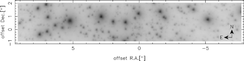
Figure 1: Ks-band field-of-view, one channel of the Wollaston prism.

Tanner et al. (2002) described IRS 21 as a bow-shock most likely created by a mass-losing Wolf-Rayet star. The observed polarization is a superposition of foreground polarization and source intrinsic polarization. It is still unclear what process(es) cause the latter component: (Mie)-scattering in the dusty environment of the Northern Arm and/or emission from magnetically aligned dust. The latter is known to occur at 12.5 $\mu$m (Aitken et al., 1998), but should be negligible at shorter wavelengths.

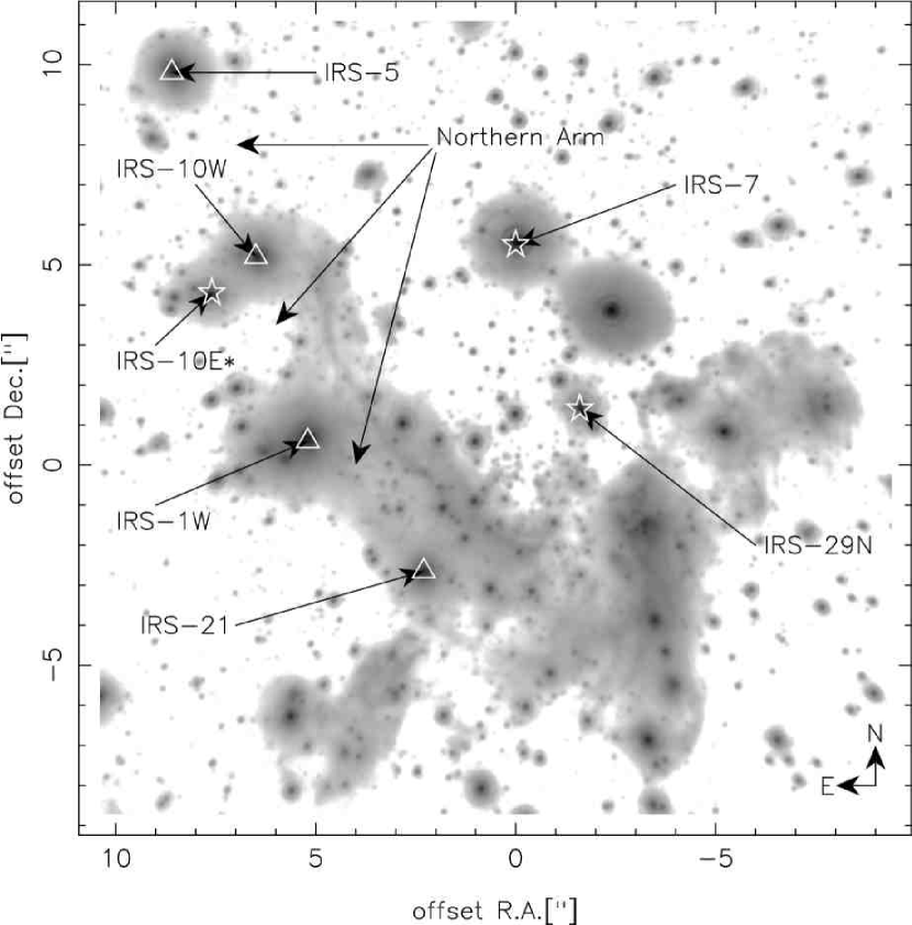
Figure 2: Lp-band image of the innermost 20” of the GC (ESO VLT NACO image, program 179.B-0261(A)). Prototypical (bow-shock) sources and location of the Northern Arm are indicated. Stellar sources are marked with stars, bow-shocks are indicated by triangles.

In general, three effects can produce polarized NIR radiation in GC sources: (re)emission by heated, non-spherical grains, scattering (on spherical and/or aligned non-spherical grains) and dichroic extinction by aligned dust grains. The first two cases can be regarded as intrinsic to the source for our purposes, thereby allowing conclusions about the source itself and its immediate environment, while the third effect is the result of grain alignment averaged along the LOS. For sources enclosed in an optically thick dust shell, dichroic extinction can also contribute significantly as a local effect (see e.g. Whitney & Wolff, 2002).
As the basic mechanism that could cause the observed large-scale grain alignment, Davis & Greenstein (1951) suggested paramagnetic dissipation, which basically aligns the angular momentum of spinning grains with the magnetic field. But even almost 60 years later, the problem of grain alignment is by no means completely solved, and it remains difficult to reach exact conclusions for dust parameters and magnetic field strength, but at least determining the magnetic field orientation is possible. If the parameters change along the LOS, this further complicates the issue. See e.g. Purcell et al. (1971), Lazarian (2003), citelazarian2007 and references therein for a review of the different possible causes of grain alignment expected to be relevant in different environments.
This makes it possible to use polarimetric measurements to map at least the direction of the magnetic fields responsible for dust alignment through the Davis-Greenstein effect, as e.g. Nishiyama et al. (2009, 2010) showed for the innermost 20’ resp. 2^∘ of the GC, but these studies did not cover the central parsec owing to insufficient resolution.
Observations of the Galactic Center suffer from strong extinction caused by dust grains on the LOS, with values of up to $A_{V}=40$ mag at optical wavelengths (or even higher values of up to 50 mag if a steeper extinction law is assumed) and still around 3 mag in the Ks-band (e.g. Scoville et al., 2003; Schödel et al., 2010b). The aligned interstellar dust grains responsible for the polarization cause extinction as well, but non-aligned grains can also contribute. Therefore, the same particles are not necessarily responsible for both effects (e.g. Martin et al., 1990). Universal power laws have been claimed for NIR extinction by Draine (1989) and polarization (Martin et al., 1990), who also showed that the law applicable to polarization in the optical domain (Serkowski et al., 1975) is a poor approximation in the NIR. The power law indices presented in these works for the extinction and the polarization power law are almost the same (1.5-2.0). It also appears that there is a correlation between the measured extinction of an intrinsically unpolarized source and foreground polarization (Serkowski et al., 1975), but this relation is quite complex. In the light of new results for the extinction law, which seem to deviate consistently from the Draine law (e.g. Gosling et al., 2009; Schödel et al., 2010b), new polarimetric measurements may be useful to further clarify the relation between extinction and polarization.

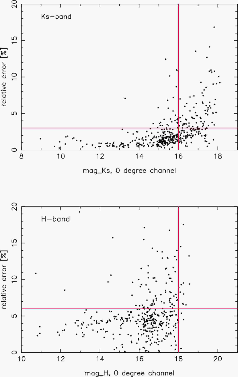
Figure 3: Total relative flux errors of the sources detected in the Ks- (upper frame) resp. H-band (lower frame). Only the 0^∘ channel is shown here, but the error distribution is very similar in the other three channels. The values are based on variations between the fluxes measured for the same source at different dither positions. The red lines denote the 16/18 mag resp. 3/6% upper limits (see Appendix A).

The central parsec of the GC is a well-suited but challenging environment to study this relation, because it contains a huge number of sources that exhibit large variances in extinction (1-2 mag, see Buchholz et al., 2009; Schödel et al., 2010b), which is produced along a long line-of-sight by a great number of dust clouds with possibly different grain alignment and composition. We are using a new Ks-band extinction map of the central parsec recently been presented by Schödel et al. (2010b).
The aims of this work are to present the first map of stellar H- and Ks-band polarization of the central few arcseconds, a highly crowded region with more than 10 sources per arcsec². In order to avoid crowding and to resolve the sources individually, the resolution of an 8m class telescope is required. Especially in the H-band, no polarization measurements exist so far for individual resolved sources in the central parsec. In addition, we will present the first spatially resolved polarimetric measurements on IRS 1W and IRS 21, also resolving the bow-shock structure of IRS 21 for the first time in the Ks-band. Furthermore, we will conduct a variability analysis on the extended sources IRS 1W, 5, 10 and 21 in the H-, Ks- and L-band.
In §2 we discuss the photometric methods used and the calibration applied to the data. Our results will be presented in §3, followed by a summary and discussion of their implications in §4.

2 Observation and data reduction

2.1 Observation

The polarimetric datasets used here were obtained using the NAOS-CONICA (NACO) instrument at the ESO VLT unit telescope 4 on Paranal in June 2004 (H-band broadband filter, program 073.B-0084A, dataset 1, see Tab.3) and May 2009 (Ks-band broadband filter, program 083.B-0031A, dataset 2). We also used several additional polarimetric Ks-band datasets contained in the ESO archive (datasets 3-15) that covered IRS 21 as well through a rotated field-of-view (FOV). Please see Tab.3 for details on the individual observations. For our variability study of the bow-shock sources we used NACO imaging data taken between June 2002 and May 2008 (H-, Ks- and L’-band data contained in the ESO archive).

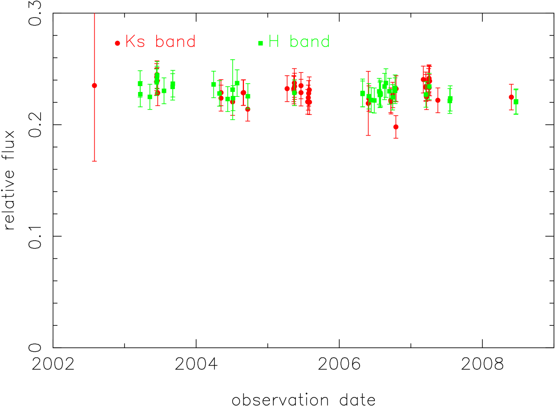
Figure 4: H- (green) and Ks-band (red) lightcurve of the known non-variable source IRS 16C.

The seeing during the polarimetric Ks-band observations was excellent with a value of $\sim$0.5”, while conditions during the H-band observations were less optimal with a seeing of $\sim$0.8”. We used the bright super-giant IRS 7 located about 6” north of Sgr A* to close the feedback loop of the adaptive optics (AO) system, thus making use of the infrared wavefront sensor installed with NAOS. The sky background was determined by taking several dithered exposures of a region largely devoid of stars, a dark cloud 713” west and 400” north of Sgr A*. The Wollaston prism available with NACO in combination with a rotatable half-wave plate was used for the polarization measurements. The two channels produced by the Wollaston prism (0^∘ and 90^∘), combined with two orientations of the half-wave plate (0^∘ and 22.5^∘), yielded four sub-images for each of several dither positions along the east-west axis. In total, we were able to cover a field-of-view of 3”$\times$16.5” (Ks-band) respectively 3”$\times$19” (H-band), corresponding to 0.12 pc $\times$ 0.66 pc and 0.12 pc $\times$ 0.72 pc, respectively (see Fig.1).
All images were corrected for dead/hot pixels, sky-subtracted and flat-fielded. It is essential for a correct calibration that the flat-field observations are taken through the Wollaston, because the flat-field shows variations caused by different transmissivity of the channels as well as effects of the inclined mirrors behind the prism (see Witzel et al., 2011, for details on these effects). Using a flat-field taken without the Wollaston prism can produce offsets in the order of 2% and 10^∘ in the measured polarization parameters. Fig.1 shows the region covered by the final mosaic that was used for the polarimetry.

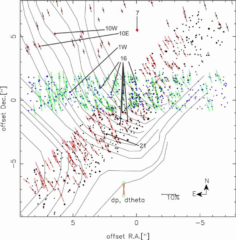
Figure 5: Ks-band polarization map of stars in the Galactic center. Only reliably measured polarization values are shown here. Blue circles and green lines: dataset 2. Black circles and red lines: dataset 4. The diameter of the circles corresponds to the brightness of the source. For comparison, we also show preliminary results of new observations taken in March 2011 (denoted by red circles and black lines). Typical errors are indicated by error cone (lower center). Thin black lines in the background denote magnetic fields determined from MIR data (Aitken et al., 1998, , based on a 1.5” beam). The brightest sources are also indicated.

The data used here were originally taken to examine flares of Sgr A* (see e.g. Eckart et al., 2006; Meyer et al., 2006; Zamaninasab et al., 2010), and this purpose requires the highest possible time resolution. This is the reason why differential polarimetry could not be applied. This technique can eliminate or reduce many instrumental effects and thus increase precision by rotating the imager by 90^∘ between exposures and thus canceling these effects out (effectively switching the 0 and 90^∘ channels). But this also means more time is needed for each exposure, because two images have to be taken for one data-point and the actual rotating takes time as well.

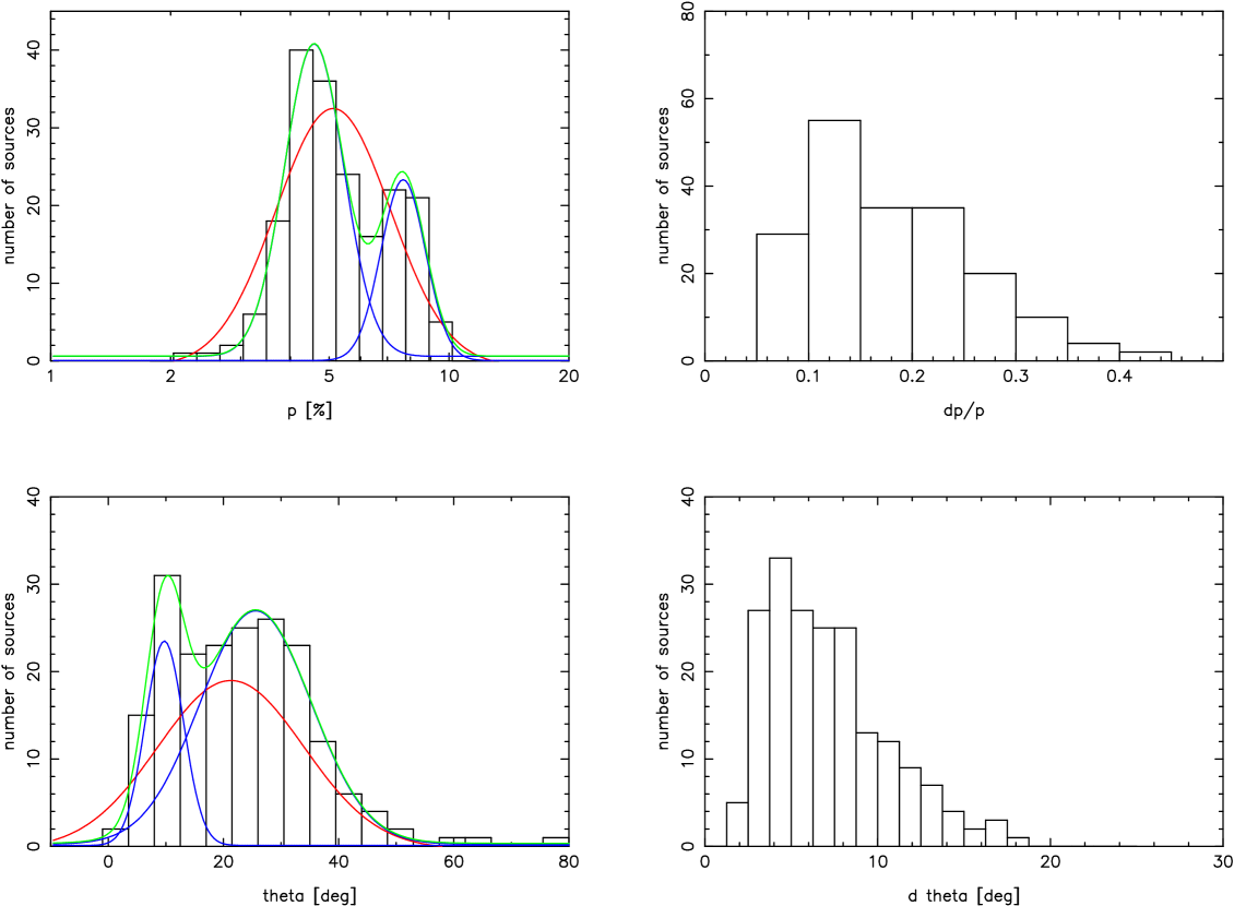
Figure 6: Ks-band polarization degrees (plotted on logarithmic scale, upper left) and angles (lower left) of stars in the Galactic Center (2009-05-18, dataset 2). The red line denotes the fit with one Gaussian distribution, while the green resp. blue lines denote the fit with a double Gaussian (green: sum, blue: individual Gaussians). Upper right: relative errors of the polarization degrees. Lower right: absolute errors of the polarization angles.

2.2 Photometry

2.2.1 Deconvolution-assisted large-scale photometry

For all datasets, the individual exposures were combined to a mosaic. All photometry was conducted on these mosaics.
Accurate photometry is crucial for polarimetry, especially when the polarization of the targets is of just a few percent. This is the case for the sources in the central parsec in the H- and Ks-band, and the effects of crowding and variations of the point-spread-function (PSF) over the FOV complicate photometry even more. For the very bright sources in the FOV, such as the IRS-16 and IRS-1 sources and the extended sources IRS-21 and IRS-1W, crowding is not a problem, but saturation can lead to additional complications. These effects have to be countered effectively in order to achieve low photometric errors.
We therefore adopted a photometric method recently presented by Schödel (2010a): first, we used the StarFinder IDL code (Diolaiti et al., 2000) to repair the cores of saturated sources (only necessary for some very bright sources in the H-band image) and extract a PSF on the full image from sufficiently bright and isolated sources. For this first step, the most suitable source would be the guide star IRS 7 itself, since it is several magnitudes brighter than any source within several arcseconds, but this source was not covered by the FOV of our dataset. We used a PSF determined from several IRS 16 and IRS 1 sources instead. Unfortunately, the most suitable of these sources were only contained in the FOV of the Ks-band data, but not covered in the H-band. Since this process is designed to determine the faint wings of the PSF accurately (see Buchholz et al., 2009; Schödel, 2010a), it works worse the fainter the initially used PSF sources are.
We used this PSF for a linear deconvolution, i.e. a division in Fourier space, followed by the application of a Wiener filter. We then applied local PSF fitting photometry by using StarFinder on overlapping sub-frames of the deconvolved image ($\sim$3”$\times$10.6”, using wider sub-fields than Schödel (2010a), this generates large overlapping regions and ensures that enough bright sources are contained in each subfield for the PSF estimation). This method significantly reduces source confusion and also minimizes systematic errors introduced by variations of the shape of the PSF over the FOV due to anisoplanasy. Despite the relatively narrow FOV, this effect still occurs because the distance and the angle to the guide star change considerably over the field. While using narrower sub-fields might counteract this, the availability of sufficiently bright PSF stars takes precedence, since this factor is the primary limit for the quality of the photometry.
The resulting fluxes in all four channels were normalized to an average of one over all channels for each source and then merged to a common list of sources detected in all channels of each sub-frame. The sub-frame lists were then merged to a common list of all detected sources.
Fig.3 show the photometric uncertainties in the H- and Ks-band. We only used sources brighter than 16 mag (Ks-band) respectively 18 mag (H-band) and with relative photometric errors of less than 3% resp. 6% in the subsequent analysis. The lower brightness limit was chosen to avoid problems with insufficient completeness and unreliable photometry, because the errors increase drastically for fainter sources. Please see Appendix A for details on our error estimation and the reasons for the error threshold.

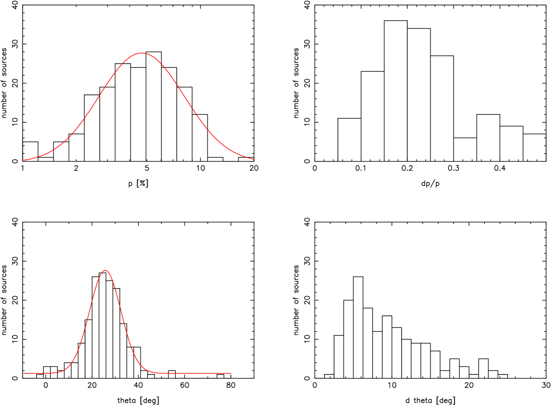
Figure 7: Ks-band polarization degrees (plotted on logarithmic scale, upper left) and angles (lower left) of stars in the Galactic Center (2007-04-03, dataset 4). The red lines denotes fits with a Gaussian distribution. Upper right: relative errors of the polarization degrees. Lower right: absolute errors of the polarization angles.

2.2.2 Photometry on extended sources

Applying the PSF fitting algorithm to extended sources leaves large residua, and a simple core-subtraction with a stellar PSF does not counter any distortions of the extended component produced by the atmosphere and the telescope. But high precision is necessary here as well. We therefore used a different approach: we deconvolved a small region of the mosaic images with the Lucy-Richardson algorithm (the ”ringing” produced by the linear deconvolution complicates the photometry of extended features), using the PSF estimated from the complete mosaic. This resulted in a much clearer view of the extended features (see Fig.18), while other sources in the vicinity appear point-like.
We shifted the resulting images to a common reference frame. We then covered the extended features with overlapping apertures ($\sim$ 27 mas radius), measuring the flux in each aperture. From these fluxes we determined the polarization at the position of the apertures. For comparison, the same method was applied to the PSF used for the deconvolution (see Appendix B). In addition, we determined the total polarization of the two known extended sources in our FOV, IRS 1W and IRS 21, by covering them with apertures of 0.25” radius. This allowed a comparison to previous observations.
In order to study a possible flux variability of the extended sources (see §3.6), we used 45 Ks-band and 38 H-band NACO datasets contained in the ESO archive (taken between 2003 and 2008). Where the bright point-sources were saturated, we used StarFinder to repair their cores. We then applied aperture photometry to the extended sources and several known bright non-variable sources (see Ott et al., 1999; Rafelski et al., 2006), with additional apertures placed on regions devoid of stars close to the targets to obtain a background estimate. This background was subtracted from the recovered fluxes and the result normalized to the total flux of the chosen non-variable calibration sources for each dataset (the IRS 16 sources except 16SW and 16NE and the IRS 33 sources; IRS 16NE is strongly saturated, while IRS 16SW has been described as an eclipsing binary and therefore shows strong flux variabilities, making it unsuitable as a reference source, see Ott et al., 1999; Rafelski et al., 2006). We estimated the uncertainty of each flux measurement by repeating the aperture photometry on the individual non-mosaiced images of each dataset (which can be assumed to be independent measurements), and adopted the standard deviation of the recovered fluxes as the total flux error. Especially for bright and isolated sources, this yields very small statistical errors on the order of less than 0.5%. We still find systematic variations of the measured fluxes on the order of about 5% between the epochs even for sources known to be non-variable on the timescale used here (see Fig.4). The latter value provides a more realistic estimate of the photometric accuracy, so we introduced an additional flux error of 5% for all data-points to be able to separate real variability from noise.

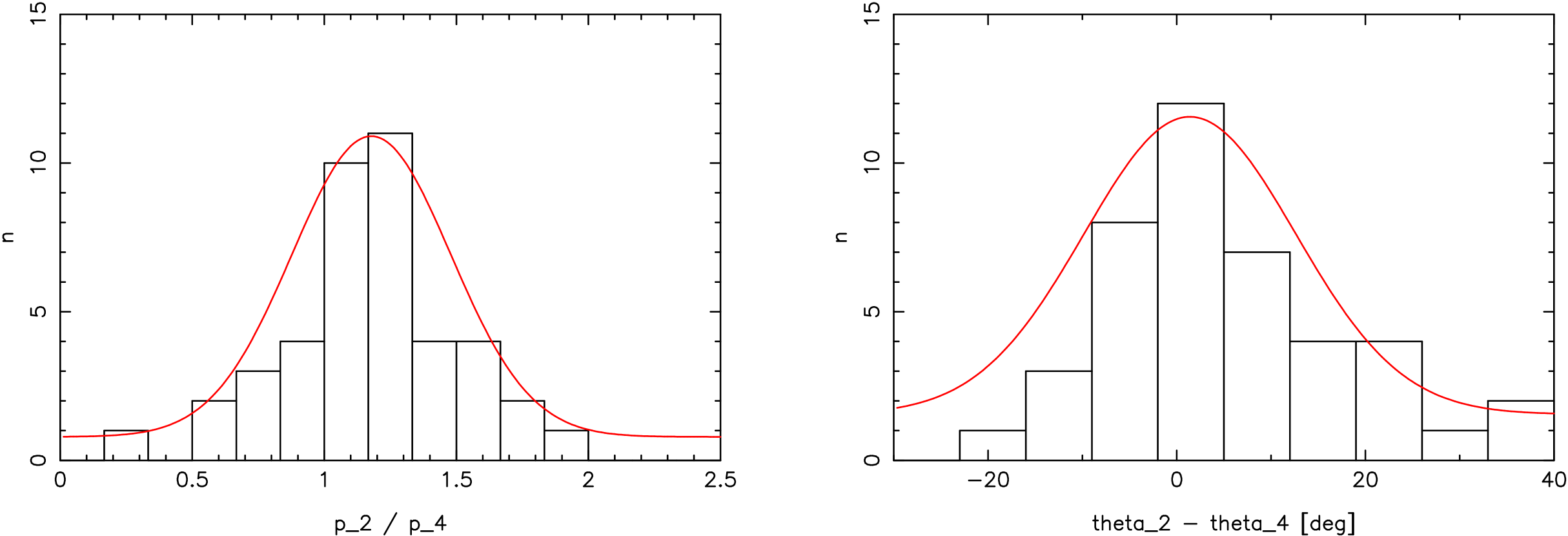
Figure 8: Comparison between polarization degrees (left frame) and angles (right frame) measured on sources common to dataset 2 (2009) and dataset 4 (2007). Plotted are histograms of $\frac{p_{2}}{p_{4}}$ resp. $\theta_{2}-\theta_{4}$, with Gaussians fitted to both values (red lines).

2.3 Polarimetry

We determined the polarization degree and angle of each source by converting the measured normalized fluxes into normalized Stokes parameters:

$$I = 1$$

$$Q = \frac{f_{0}-f_{90}}{f_{0}+f_{90}}$$ (1)

$$U = \frac{f_{45}-f_{135}}{f_{45}+f_{135}}$$ (2)

$$V = 0.$$

Because NACO is not equipped with a $\frac{\lambda}{4}$ plate, it was not possible to measure circular polarization. However, Bailey et al. (1984) showed that the circular polarization of sources in the GC is at best very small, so we assume here that it can be neglected and set to 0 at our level of accuracy. Polarization degree and angle can then be determined as

$$P = \sqrt{Q^{2}+U^{2}}$$ (3)

$$\theta = 0.5\times atan\left(\frac{U}{Q}\right).$$ (4)

Errors for I, Q, U and subsequently p and $\theta$ were determined from the flux errors. In order to determine whether or not the polarization of a source was determined reliably, we calculated the normalized fluxes that would be expected for the determined values of p and $\theta$. The difference between these values and the measured fluxes was then compared to the photometric errors of each data-point. The source was only classified as reliable if the root-mean-square of the deviations did not exceed the root-mean-square of the relative photometric errors. The subsequent analysis is only based on these higher quality sources.

2.4 Calibration of the measured polarization

A first comparison of our measurements to known values (Knacke & Capps, 1977; Bailey et al., 1984; Eckart et al., 1995; Ott et al., 1999) revealed significant offsets, especially in the polarization angles. Instead of the expected orientation along the galactic plane (oriented $\sim$31.4^∘ East-of-North, in the following, positive angles should be read as East-of-North, negative as West-of-North), we found orientations of the polarization vectors of about -5^∘. The problem that surfaces here is that NACO was not specifically built for polarimetry, so instrumental effects like this can be expected and have to be countered by a special calibration. Also, the observation technique was developed for the study of short-term variabilities (flares) of Sgr A* and not for high-precision polarimetry on stellar sources.
To reduce this problem, Witzel et al. (2011) developed an analytical model of the behavior of polarized light within NACO. It consists of Müller matrices to be applied to the measured Stokes vector of each source, which then yields the actual Stokes parameters of the source. In general, any optical effect such as reflection, transmission, polarization etc. can be described by a Müller matrix. A combination of effects as it occurs here is then represented by a multiplication of the individual Müller matrices. If the necessary material constants and the construction of the instrument are known, the resulting matrix can be used to significantly reduce systematic offsets and uncertainties. Witzel et al. (2011) show that by using this method, the systematic uncertainties of polarization degrees and angles can be reduced to $\sim$1% and $\sim$5^∘. Applied to our data, this limits the final accuracy by the photometric uncertainties instead of by instrumental effects. For a detailed description of the model and the Müller matrices themselves, see Witzel et al. (2011).
Utilizing this new calibration model means that an actual direct calibration can be achieved for the first time at this resolution. Previous studies like Eckart et al. (1995) and Ott et al. (1999) had to adopt a calibration based on reference values taken from Knacke & Capps (1977).

2.5 Correcting for foreground polarization

It can be assumed that the total effect of the foreground polarization can be treated as a simple linear polarizer with a certain orientation $\theta_{fg}$ and efficiency $p_{fg}$. This can be described by a Müller matrix:

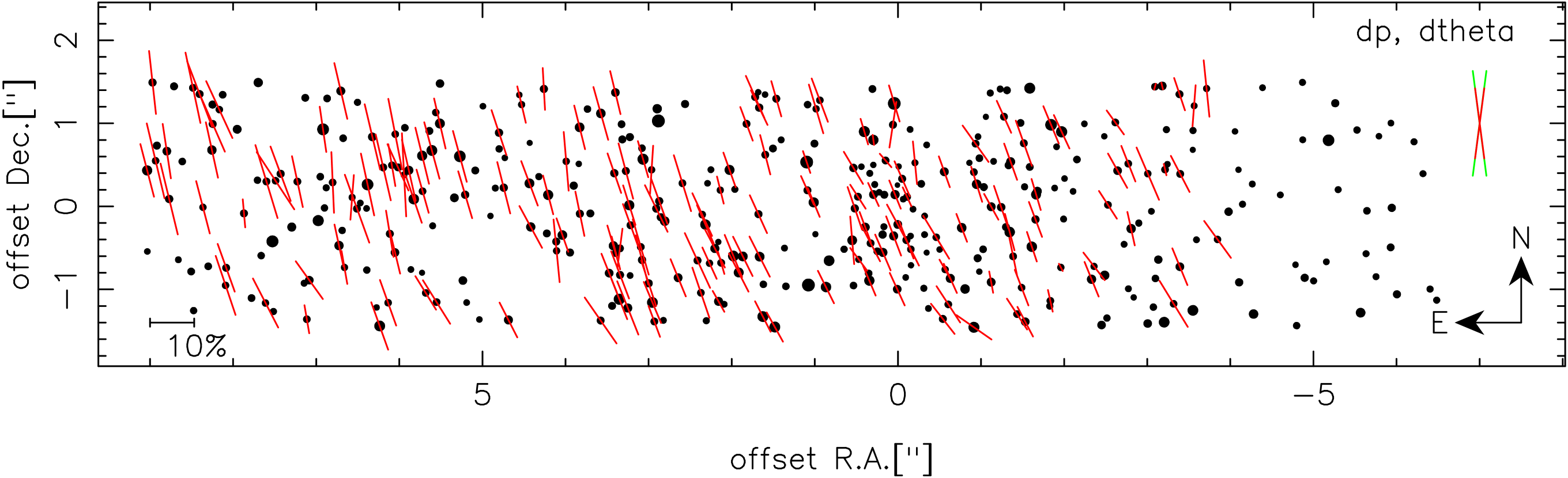
Figure 9: H-band polarization map of stars in the Galactic Center (dataset 1). Only reliably measured polarization values are shown here. Typical errors plotted as error cone (upper right), adopted from Ks-band data.

$$S_{obs} = \left(\begin{array}[]{c}I\\ Q\\ U\\ V\end{array}\right)=M_{fg}\times S_{int}=M_{fg}\times\left(\begin{array}[]{c}I^{\prime}\\ Q^{\prime}\\ U^{\prime}\\ V^{\prime}\end{array}\right)$$ (13)

$$= M_{rot}(-\theta^{\prime})\times M_{lin}(p)\times M_{rot}(\theta^{\prime})\times S_{int},$$ (14)

with $S_{obs}$ as the observed total Stokes vector and $S_{int}$ as the Stokes vector of the intrinsic polarization. $M_{lin}(p)$ is the Müller matrix describing a linear polarizer, producing a maximum of polarization along the North-South-axis:

$$M_{lin}(p)=\left(\begin{array}[]{cccc}1&-p&0&0\\ -p&1&0&0\\ 0&0&\sqrt{1-p^{2}}&0\\ 0&0&0&\sqrt{1-p^{2}}\end{array}\right)$$

. This matrix has to be rotated to the appropriate angle by multiplying it with $M_{rot}(\theta^{\prime})$, a standard 4$\times$4 rotation matrix:

$$M_{rot}(\theta^{\prime})=\left(\begin{array}[]{cccc}1&0&0&0\\ 0&cos(2\theta^{\prime})&sin(2\theta^{\prime})&0\\ 0&-sin(2\theta^{\prime})&cos(2\theta^{\prime})&0\\ 0&0&0&1\end{array}\right)$$

. $\theta^{\prime}=90^{\circ}+\theta_{fg}$ has to be used in the rotation matrix, because we define the polarization angle $\theta$ as the angle where we measure the flux maximum, while the angle of reference for the Müller matrix describing the linear polarizer is the angle where the maximum in absorption occurs.
For each source to which the depolarization matrix was applied, we used the average of the polarization parameters of the surrounding point sources as an estimate for $\theta_{fg}$ and $p_{fg}$.
The resulting matrix can then be inverted and multiplied with the calibrated observed Stokes vector of a source to remove the foreground polarization and leave only the intrinsic polarization. We applied this method to the total polarization and the polarization maps of the extended sources (IRS 21 and IRS 1W), to isolate their intrinsic polarization pattern. The relevance of the results depends heavily on the accuracy of the foreground polarization estimate.

3 Results and discussion

3.1 Ks-band polarization

2009 data (dataset 2)

We were able to measure reliable polarization parameters for 194 sources brighter than 16 mag in our main 2009 Ks-band dataset. For fainter sources, the photometric uncertainty becomes too large to determine the polarization reliably, and this limit also helps to avoid problems with insufficient completeness and source crowding, which could generate a bias in the averaged values. The subsequent analysis and the comparison to the H-band data is only based on this dataset.
The polarization angles in the central arcseconds mostly follow the orientation of the galactic plane within the uncertainty limits (31.4^∘ (Reid et al., 2004), while we find angles of $\sim$25-30^∘ for our sources). Toward the eastern edge of the FOV, we find slightly steeper angles ($\sim$5-15^∘, see Fig.5). A few sources west of Sgr A* also show similar steep angles, but there are too few reliable sources there to allow any conclusions. Here and in the following, we use the term ”steeper angle” to denote angles with an absolute value closer to 0^∘, so that an angle of 10^∘ would be steeper than one of 30^∘. The polarization angle can vary between -90^∘ and 90^∘, in the way that 91^∘ (East-of-North) corresponds to -89^∘.
The distribution of the polarization angles (see Fig.6, lower left frame) can be fitted with a single Gaussian, peaked at 20^∘ with a FWHM of 30^∘. Using the FWHM as a measure for the uncertainty (with $\sigma=\frac{FWHM}{2\sqrt{2\times ln(2)}}$), this yields $\theta=20^{\circ}\pm 13^{\circ}$. Using a fitting function with two Gaussian peaks yields a significantly lower $\chi^{2}$ (by a factor of 3). The two peaks are fitted at $\theta_{1}=10^{\circ}\pm 4^{\circ}$ (FWHM of 10^∘) respectively $\theta_{2}=26^{\circ}\pm 8^{\circ}$ (FWHM of 20^∘). Considering the uncertainties of the polarization angles shown in the lower right frame of Fig.6, which are on the order of up to 15^∘, it can be questioned if these two peaks are indeed a real feature, with the distance between the peaks on the order of these typical errors.
The polarization degree also appears to vary over the field, with values of 4-5% in the central region and 8-10% toward the eastern edge (and for some western sources, but with the same caveat as for the polarization angle). Especially sources in the area around the IRS 1 sources show these higher polarization degrees. We fitted the logarithms of the polarization degrees with a Gaussian (peaked at (5.1 $\pm$ 1.7)%, FWHM of 4.0%, see Fig.6, upper left frame), and like the single Gaussian fit to the polarization angles, the fit was quite poor. Repeating the fit with a double Gaussian yielded two peaks at (4.6 $\pm$ 0.8)% respectively (7.7 $\pm$ 1.2)%, with FWHMs of 1.8% resp. 2.8% and a significantly better $\chi^{2}$ (by a factor of 8). The relative uncertainties of the polarization degree are on the order of up to 30% (see Fig.6, upper right frame), and this limits the confidence in the two fitted peaks.
Comparing the two fitted Gaussian distributions for both parameters, we find a similar number of stars contained in the 10^∘ and the 7.7% peak ($\sim$25-30%), resp. the 26^∘ and 4.6% peak ($\sim$70-75%). This confirms the general trends found in Fig.5 and indicates that the fitted peaks indeed correspond to a real feature.
We plotted the Ks-band polarization degrees versus the polarization angles in Fig.11, left frame, and there appears to be a trend that higher polarization degrees coincide with steeper polarization angles, despite the large errors.

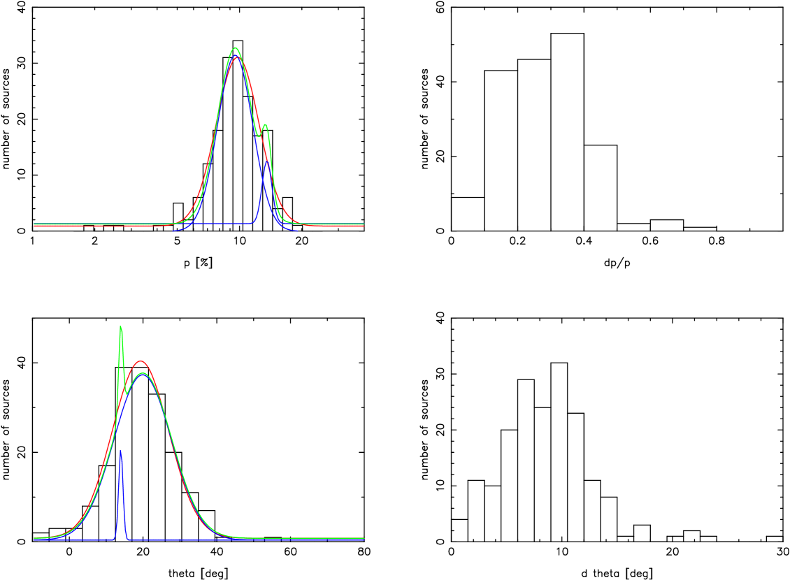
Figure 10: H-band polarization degrees (plotted on logarithmic scale, upper left) and angles (lower left) of stars in the Galactic Center (dataset 1). The red line denotes the fit with one Gaussian distribution, while green resp. blue lines denote the fit with a double Gaussian (green: sum, blue: individual Gaussians). Upper right: relative errors of the polarization degrees. Lower right: absolute errors of the polarization angles.

2007 data, rotated FOV (dataset 4)

We measured reliable polarization parameters for 186 sources brighter than 16 mag. This dataset has a lower Strehl ratio (on average) than the 2009 data (22% compared to 27%). We used this dataset only for comparison with the main Ks-band data (dataset 2, with the main purpose to determine the presence of unaccounted instrumental effects over the FOV), since no H-band data with this FOV is available.
The trends we find here are similar to those in the main dataset: the polarization angles appear to be aligned with the Galactic plane (see Fig.5), but we do not observe the same shift in polarization angle toward the east of the FOV. We do, however, find an increase in polarization degree toward the southeast, similar to the increase found in the 2009 data toward the east. Both the distribution of the polarization degrees (logarithmic) and the polarization angles can be fitted with a single Gaussian with sufficient accuracy (see Fig.7), with peaks fitted at (4.6 $\pm$ 2.1)% respectively $26^{\circ}\pm 8^{\circ}$ (FWHM of 5% resp. 20^∘). The FWHM of the distribution of the polarization degrees is comparable to that found for the 2009 data, but a single Gaussian provides a much better fit here. The larger uncertainties would however lead to a blurring of the two Gaussians, if indeed two were present.
The relative errors of the polarization degree (see Fig.6, upper right frame) mostly stay below 30%, with some outlier values of up to 40-50%. This exceeds the errors found for dataset 2, but this can be expected because of the lower data quality. The errors found for the polarization angles are also larger on average than those measured for dataset 2.
The sources in the overlapping area of dataset 2 and 4 for which reliable measurements could be obtained in both datasets show very similar polarization parameters (see Fig.8). We find that the polarization degrees and angles of 82% of the common sources agree within 1 sigma, viewing the parameters individually. Both parameters agree within 1 sigma for 69% of the common sources. For 93% of the common sources both parameters agree within 2 sigma, and 98% (all but one source) show an agreement within 3 sigma.
We fitted the relation between the polarization degrees resp. the difference of the polarization angles of the sources in the common region of both datasets with a Gaussian (see Fig.8). We fitted the peaks at $\frac{p_{2}}{p_{4}}=1.2\pm 0.2$ (FWHM of 0.5) and $\theta_{2}-\theta_{4}=1^{\circ}\pm 7^{\circ}$ (FWHM of $17^{\circ}$). The uncertainties of these values provide an estimate for the general accuracy of the Ks-band measurements, so we plotted them as an error cone in Fig.5.
This reinforces the confidence in the measured values in both datasets, while it also provides a confidence limit. A $3\sigma$-deviation would correspond to a (relative) 60% offset in polarization degree and a difference of 21^∘ in polarization angle.
Unfortunately, the overlapping part of the FOVs is only about 8 arcsec², and no data with a different FOV exist for the regions that show an excess in polarization degree/angle in both datasets.
Fig.5 also shows the preliminary results of new polarization measurements (program 086.C-0049(A)) of a region north of the FOV of dataset 2. These measurements seem to link up well with the findings in dataset 2 and 4. A detailed analysis of these observations will be the subject of a future study.

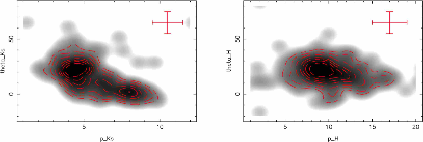
Figure 11: Polarization angle vs. polarization degree, plotted as logarithmic smoothed point density, with typical error indicated by red bars (upper right corners). Contours were plotted to guide the eye. Left frame: Ks-band, right frame: H-band

3.2 H-band polarization

Reliable results could be obtained for 163 sources brighter than 18 mag. The limit of 18 mag was chosen because this corresponds to the limit of 16 mag in the Ks-band, assuming a typical H-Ks of $\sim$2 (with H-Ks${}_{intrinsic}\sim$0 and A_H-A${}_{Ks}\sim$2, see e.g. Schödel et al., 2010b). The lower number of sources with reliable polarization compared to the Ks-band can be attributed to the significantly lower Strehl ratio of the H-band data (0.17 compared to 0.27 in the Ks-band) and the slightly different FOV, but the latter is a minor effect. We find polarization angles very similar to those in the Ks-band, but with a more uniform distribution over the FOV (see Fig.9). The distribution of the polarization angles can be fitted well with a single Gaussian, peaking at $20^{\circ}\pm 8^{\circ}$ (FWHM of 19^∘, see Fig.10, lower left frame). Fitting this distribution with a double Gaussian produces a slightly better $\chi^{2}$, but this can be expected for an increase in the number of fitting parameters. A single Gaussian fits the distribution with sufficient accuracy, compared to the poor fit with a single Gaussian function for the Ks-band polarization angles. We find typical errors of the polarization angle of up to 12^∘ (see Fig.10, lower right frame).
The polarization degree also appears to be quite uniform over the FOV, with typical values of 8-12%. Fitting the logarithms of the polarization degrees with a single Gaussian leads to a peak at (9.8 $\pm$ 0.7)% (FWHM of 1.7%), satisfyingly matching the data (see Fig.10, upper left frame). We also fitted the data with two Gaussian peaks for comparison, but this only marginally improves the fit. We find relative uncertainties of the polarization degree on the order of up to 40% (see Fig.10, upper right frame).
Unfortunately, no high-resolution H-band measurements with a different FOV are available for a comparison.
As for the Ks-band, we plotted the H-band polarization degrees versus the polarization angles (see Fig.11, right frame). No large-scale trend is visible, both parameters appear concentrated around $\sim$20^∘ resp. $\sim$9%.

3.3 Comparison to previous results

We compared the polarization degrees and angles of 30 sources from Eckart et al. (1995) and 13 sources from Ott et al. (1999) to the values we determined from our data. These two studies were calibrated based on polarization parameters determined by Knacke & Capps (1977) and Lebofsky et al. (1982). We find that 87% of the Eckart sources agree with our values within 3 sigma in polarization degree (and 83% in polarization angle). For the Ott sources (with a slightly different FOV) we find that 77% agree with our own values within 3 sigma for both polarization degree and angle. Differences between these older studies and our own measurements can probably be attributed to the lower spatial resolution of the former. Both older studies show average polarization angles generally parallel to the Galactic plane, on average at 25^∘ resp. 30^∘. We find similar results for our much larger number of sources. The average polarization degree is slightly higher, but this can be expected because the inclusion of IRS 7 with its polarization degree of only 3.6% in both older surveys considerably lowered the flux-weighted average that was calculated there.
One other thing has to be considered here: we have for the first time applied an absolute polarimetric calibration to high angular resolution data. That we find such good agreement with data where a relative calibration based on the Knacke & Capps (1977) values was used increases the confidence in both this study and the results of the mentioned previous works.
The only direct possibility to compare our study with the results of Knacke & Capps (1977) exists in the vicinity of IRS 1. There, we find a flux-weighted average polarization of $4.3\pm 0.5$% at $14^{\circ}\pm 10^{\circ}$ in a 3.5” aperture, which matches the value given in the older study ($3.5\pm 0.5$% at $16^{\circ}\pm 5^{\circ}$). We calculated the flux-weighted average by summing the fluxes of the individual stars contained in the aperture for each channel and calculating Q and U (and subsequently p and $\theta$) from these total values. This corresponds to a flux-weighted average over Q and U.
The reason why this value is much lower than the polarization generally found in this area is the contribution of IRS 1W with its high flux and an intrinsic polarization which is almost perpendicular to that of the sources in the vicinity.
This additionally supports our findings of higher polarization degrees toward the eastern edge of the FOV: for the total polarization to be on the order of 4% (including IRS 1W), the surrounding sources must have a significantly higher polarization degree.
We compared our findings to several older NACO data-sets with the same FOV. Using aperture photometry on the IRS 1 sources (except IRS 1W) and the northern IRS 16 sources except IRS 16NW (to avoid problems with saturation), we found average offsets in both polarization degree and angle in the order of 10-15^∘ and 2-3%, with higher polarization degrees and steeper polarization angles for the IRS 1 sources. This again confirmed the trends we find in our main data-set.
Very few H-band polarization measurements are available for a comparison. The most recent survey with an aperture not exceeding our FOV was conducted by Bailey et al. (1984) in the J-, H- and K-band, who present polarization parameters for two sources in our FOV, IRS 1 and IRS 16 (treating these complexes as a single source each, using a 3.0” aperture). That study measured $9.9\pm 0.6$% at $20^{\circ}\pm 1^{\circ}$ for IRS 1 respectively $10.2\pm 0.2$% at $8^{\circ}\pm 1^{\circ}$ for IRS 16 in the H-band. Calculating a flux weighted average in a 3.0” aperture around the IRS 1 resp. IRS 16 sources based on our data yields values of $10.9\pm 0.5$% at $15^{\circ}\pm 10^{\circ}$ for IRS 1 and $7.2\pm 0.5$% at $21^{\circ}\pm 10^{\circ}$ for IRS 16. This agrees well for IRS 1, while the polarization degree found for IRS 16 deviates considerably. But it has to be considered that both sources were only very poorly resolved at the time of that study, not all IRS 16 sources are contained in our FOV, and we only used sources with reliably measured polarization for the comparison.
Our measured polarization degrees and angles are also compatible to the larger-scale polarization maps presented by Nishiyama et al. (2009) in the H- and the Ks-band. The authors find polarization angles of $\sim$20^∘ in the area around our own FOV, which itself is not covered in that study.

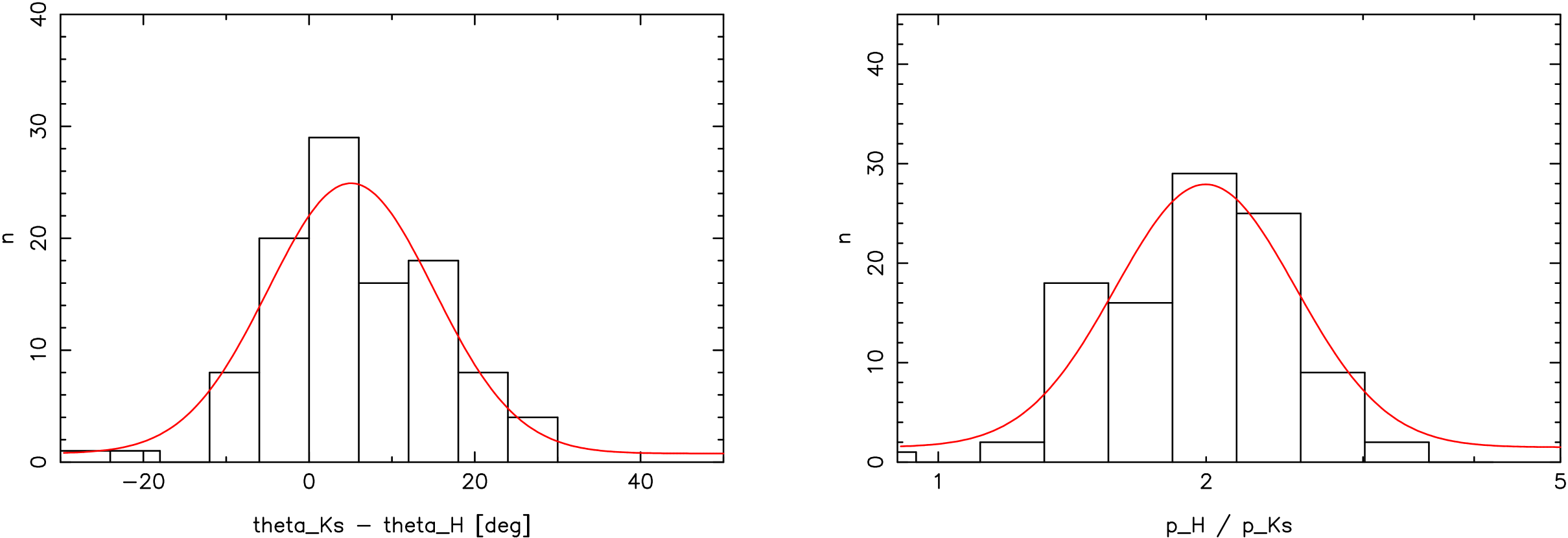
Figure 12: Left frame: difference between H- and Ks-band polarization angle. Right frame: relation of H- to Ks-band polarization degree (logarithmic plot). The red line represents a Gaussian fitted to the histograms.

3.4 Relation between H- and Ks-band polarization

Table 1: Results of Gaussian fits to polarization parameter histograms for the complete dataset resp. sub-datasets separated based on $p_{Ks}$ resp. position along the East-West-axis. Polarization degrees given in %, angles given in degrees.

separation	value	peak 1	$\sigma_{1}$	peak 2	$\sigma_{2}$
none	$p_{Ks}$[%]	4.6	0.8	7.7	1.2
none	$p_{H}$[%]	9.8	0.7
none	$\theta_{Ks}[^{\circ}]$	28	3	12	6
none	$\theta_{H}[^{\circ}]$	20	8
none	$\frac{p_{H}}{p_{Ks}}$	1.9	0.4
none	$\theta_{H}-\theta_{Ks}[^{\circ}]$	2	8
$p_{Ks}$	$p_{Ks}$[%]	4.6	0.6	7.5	1.0
$p_{Ks}$	$p_{H}$[%]	9.3	1.3	12.1	2.1
$p_{Ks}$	$\theta_{Ks}[^{\circ}]$	28	6	11	6
$p_{Ks}$	$\theta_{H}[^{\circ}]$	20	6	13	6
$p_{Ks}$	$\frac{p_{H}}{p_{Ks}}$	2.0	0.3	1.6	0.3
$p_{Ks}$	$\theta_{H}-\theta_{Ks}[^{\circ}]$	-5	4	4	5
E-W pos	$p_{Ks}$[%]	4.6	0.6	7.7	1.0
E-W pos	$p_{H}$[%]	9.3	1.4	11.8	2.1
E-W pos	$\theta_{Ks}[^{\circ}]$	29	6	10	7
E-W pos	$\theta_{H}[^{\circ}]$	21	6	13	6
E-W pos	$\frac{p_{H}}{p_{Ks}}$	2.0	0.3	1.7	0.3
E-W pos	$\theta_{H}-\theta_{Ks}[^{\circ}]$	-5	4	3	5

By comparing the positions of the sources detected in each datasets, we found 133 sources with reliable polarization parameters common to the H- and the Ks-band data. The missing sources are mostly found outside the other data-set’s FOV, in addition to a small number of very fast moving sources (like the S stars), which are difficult to identify owing to the time of 2.5 years between the H- and Ks-band observations. In addition, photometric errors tend to be larger in the westernmost region of the FOV because of the lack of suitable close bright stars for PSF determination. This leads to less sources with reliable polarization parameters there. The common sources are used for the following source-by-source comparison.
We find that the polarization angles measured in the H- and Ks-band agree well in the eastern part of the FOV, while there appears to be an offset in the center and the western region. Fig.12 shows the difference in polarization angle and the relation of H- and Ks-band polarization degrees. $\theta_{H}-\theta_{Ks}$ can be fitted well with a Gaussian distribution and shows a peak at $4^{\circ}\pm 8^{\circ}$ (FWHM of 20^∘). Considering the width of the peak, this offset is not significantly different from zero. $\frac{p_{H}}{p_{Ks}}$ can be fitted quite well with a log-normal distribution, peaking at 1.9 $\pm$ 0.4 (FWHM of 0.9). For a complete list of the fitting results, see Tab.1 (which also contains the values referred to in the paragraphs below).
Assuming the two peaks we find for both the polarization degree and angle in the Ks-band are real, we separated the stars with reliable polarization parameters in both H- and Ks-band into two samples: stars with $p_{Ks}<6\%$ (pK^-) and with $p_{Ks}>6\%$ (pK⁺). Fig.13 shows histograms of the different polarization parameters of the pK^- and pK⁺ sources in the two bands, namely the polarization degrees and angles, $\theta_{H}-\theta_{Ks}$ and $\frac{p_{H}}{p_{Ks}}$. All histograms were fitted with a Gaussian, and although these fits are poor in several cases, the fitted peaks show at least the trends present in the data.
We find that the pK⁺ sources show systematically lower polarization angles than the pK^- sources in the Ks-band (peak offset of 18^∘). The peaks fitted here match the ones fitted to the complete dataset (see §3.1). A similar, yet smaller offset exists in the H-band (7^∘, well within the uncertainties, the fitted peaks also correspond to those determined in §3.2). Accordingly, $\theta_{H}-\theta_{Ks}$ also shows an offset of 9^∘, but that value is relatively close to zero for both sub-datasets considering the large FWHM of the peaks.
Looking at the polarization degrees, we find similar offsets: for the Ks-band, the pK⁺ peak is found at a polarization degree which is higher by a factor of 1.6 than where the pK^- peak is fitted. The relative difference found in the H-band is smaller, with the pK⁺ peak found at a polarization degree which is higher by a factor of 1.3 than that of the pK^- peak. This manifests itself in the $\frac{p_{H}}{p_{Ks}}$ histogram, which we find peaked at 1.6 for pK⁺, and at 2.0 for pK^-.
Because we mostly find the higher polarized pK⁺ sources in the eastern part of our FOV (in the general area of the Northern Arm), we also divided our sources into two samples based on their position along the East-West-axis: pK-E (sources more than 4.1” east of Sgr A*) and pK-W (sources less than 4.1” east of Sgr A*). Fig.14 shows histograms of the polarization parameters for both sub-datasets. We find results that are very similar to those found for a separation based on $p_{Ks}$, with practically identical peaks and offsets (pK-E corresponding to pK⁺, pK-W to pK^-).
How can we explain these findings? For interstellar polarization in general, the H-band polarization degrees are expected to be significantly higher than the Ks-band values, while the angles in both bands should be the same within the uncertainties. This is expected from the Serkowski law and the power law relation presented by Martin et al. (1990). According to the semi-empirical Serkowski law, the polarization at a given wavelength in relation to the polarization maximum depends on the wavelength where that maximum occurs

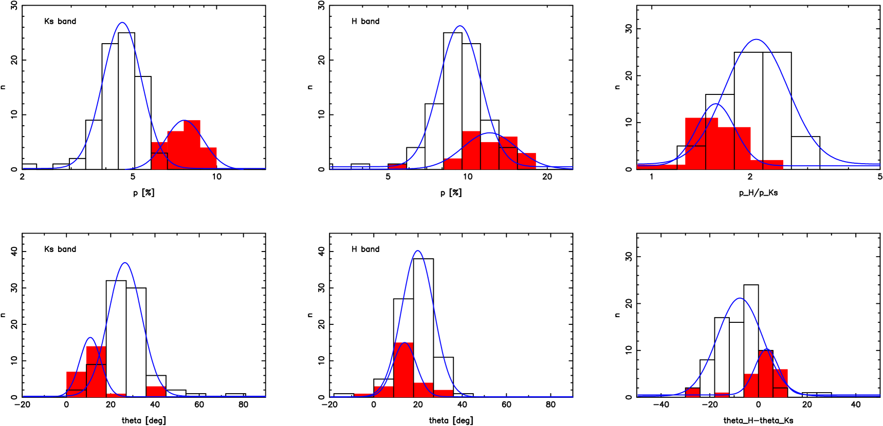
Figure 13: Sources detected in H- and Ks-band, separated by Ks-band polarization. White columns: p${}_{Ks}<6$%. Red columns: p${}_{Ks}>6$%. Upper/lower left frame: Ks-band polarization degree/angle, Upper/lower middle frame: H-band polarization degree/angle, upper right frame: relation of H- and Ks-band polarization degree (logarithmic plot). Lower right frame: difference between H- and Ks-band polarization angle. Blue lines represent Gaussian fits to the histograms.

$$\frac{p(\lambda)}{p_{max}}=exp\left[-K\times ln^{2}\left(\frac{\lambda_{max}}{\lambda}\right)\right]$$ (15)

with $K=0.01+1.66\lambda_{max}$ (Whittet et al., 1992). It appears, however, that polarization in the NIR, specifically in the J-, H- and K-band, only very weakly depends on $\lambda_{max}$ (Martin et al., 1990). Keeping this in mind and considering the availability of only two data-points for each source and the large FWHM of the Gaussian fits to $\frac{p_{H}}{p_{Ks}}$, we can only give rough estimates here. We find that the peak fitted to the complete dataset (1.9 $\pm$ 0.9) agrees best with $\lambda_{max}\sim 0.7\mu m$. Of the two fitted peaks for the sub-datasets, the value of 2.0 $\pm$ 0.7 would agree with $\lambda_{max}\sim 0.7\mu m$ as well, while the peak at 1.6 $\pm$ 0.7 points to a $\lambda_{max}$ which is either much smaller ($\sim 0.25\mu m$) or larger ($\sim 1.25\mu m$). Bailey et al. (1984) give a value of $\lambda_{max}\approx 0.80\mu m$ (using J, H-and K-band data), which approximately matches the first two values we find here. The authors state that the agreement with the semi-empirical law is only rough. It also has to be considered that this law was established for sources with only very weak polarization in the NIR, and consequently does not describe observations in that wavelength regime very well. All this leads us to conclude that our data clearly are not sufficient to give a reliable estimate for this parameter.
Using the power-law relation proposed by Martin et al. (1990)

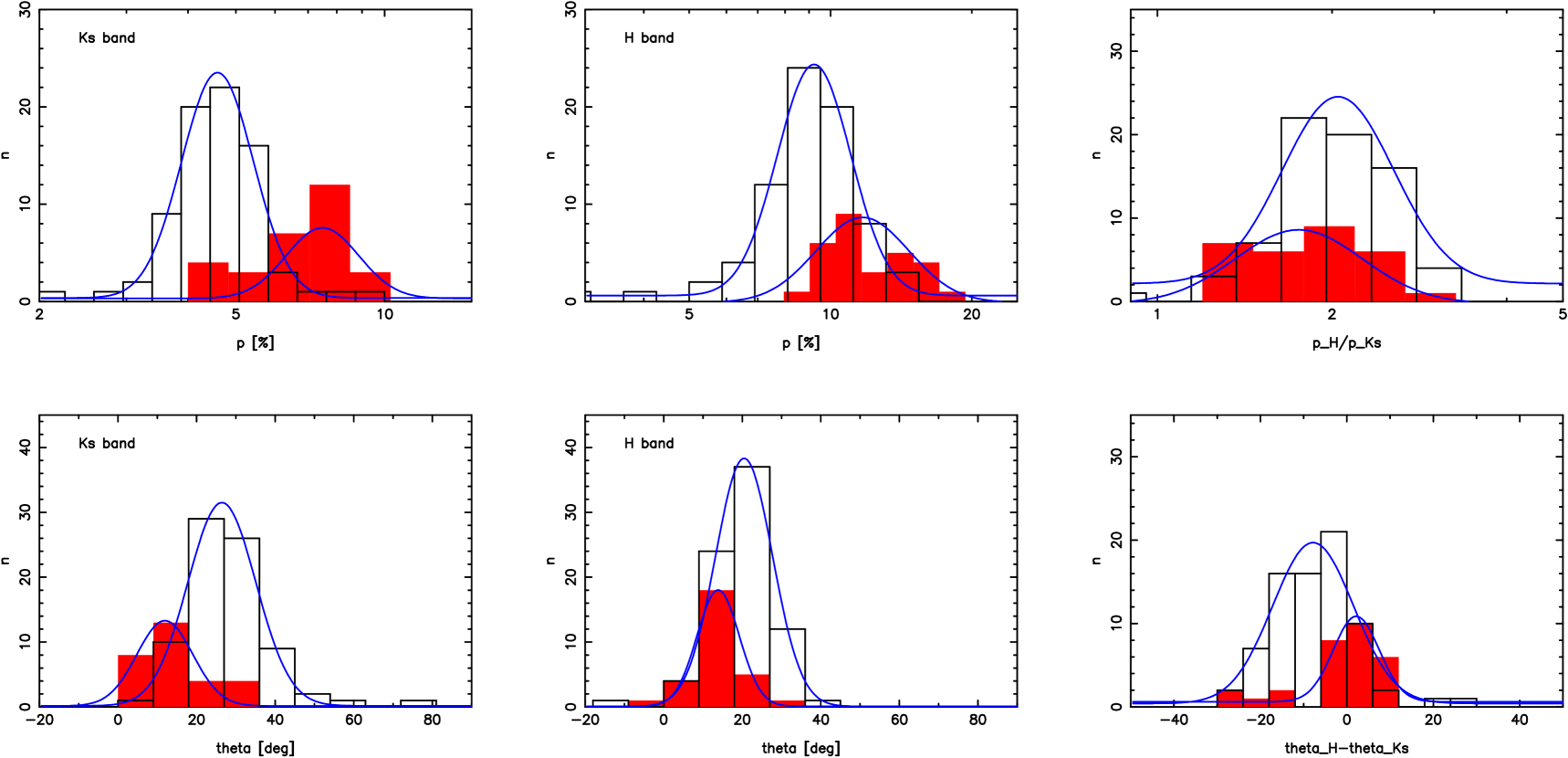
Figure 14: Sources detected in the H- and Ks-band, separated by position along the East-West-axis. White columns: sources less than 4.1” east of Sgr A*. Red columns: sources more than 4.1” east of Sgr A*. Upper/lower left frame: Ks-band polarization degree/angle, upper/lower middle frame: H-band polarization degree/angle, Upper right frame: relation of H- and Ks-band polarization degree (logarithmic plot). Lower right frame: difference between H- and Ks-band polarization angle. Blue lines represent Gaussian fits to the histograms.

$$\frac{p_{H}}{p_{Ks}}=\left(\frac{\lambda_{H}}{\lambda_{Ks}}\right)^{-\alpha}$$ (16)

we obtain a power-law index of $\alpha=2.4\pm 1.7$ for $\frac{p_{H}}{p_{Ks}}=1.9\pm 0.9$, while the two sub-dataset peaks lead to $\alpha=1.7\pm 1.6$ resp. $\alpha=2.5\pm 1.3$. These values agree with the range of 1.5-2.0 given by Martin et al. (1990), although the uncertainties are quite large. It has to be stressed that our values have been obtained on a relatively narrow region and that a study of a much wider region is necessary before any reliable conclusions can be drawn on this matter.
Fig.15 shows binned plots of the H- and Ks-band polarization parameters. Only the common reliable sources were used for this comparison. We averaged the polarization parameters for all sources contained in 1.3” wide bins along the East-West axis.
We observe the same large-scale trends found based on the histograms, and the first impression points toward the same effects being present in both Ks- and H-band for both polarization degree and angle. Looking at the plots of $\frac{p_{H}}{p_{Ks}}$ and $\theta_{H}-\theta_{Ks}$, however, the differences between the two bands become apparent: as seen in Fig.14, $\frac{p_{H}}{p_{Ks}}$ is found to be around 2-2.2 in the center and more toward 1.5-1.6 east of Sgr A*. A similar trend is visible toward the western edge, but there are few sources there and there may be an influence of edge effects. The $\theta_{H}-\theta_{Ks}$ plot also confirms the trends found earlier: we see an offset of $\sim$10^∘ in the center and the west and one of $\sim$0^∘ toward the east.
These results raise the question for the cause of the observed deviations of the polarization parameters over the FOV, assuming those deviations are indeed real and not some sort of instrumental effect we did not account for. The comparison of our main Ks-band dataset (2) with dataset 4 shows that while a similar increase in polarization degree exists there as well, no accompanying shift in polarization angle is found. If this was indeed an instrumental effect, one would expect the same pattern in both parameters. Fig.30 shows a residue of the dither pattern in both Q and U, but these variations are far too small to lead to a significant deviation over the FOV as we observe it here.
It has to be considered that the significance of the trends we find stays below $3\sigma$, based on the systematic uncertainties determined in §3.1
This question cannot be solved completely without additional (calibration) observations, but for the purposes of this study, we assume that what we observe is indeed a real effect.

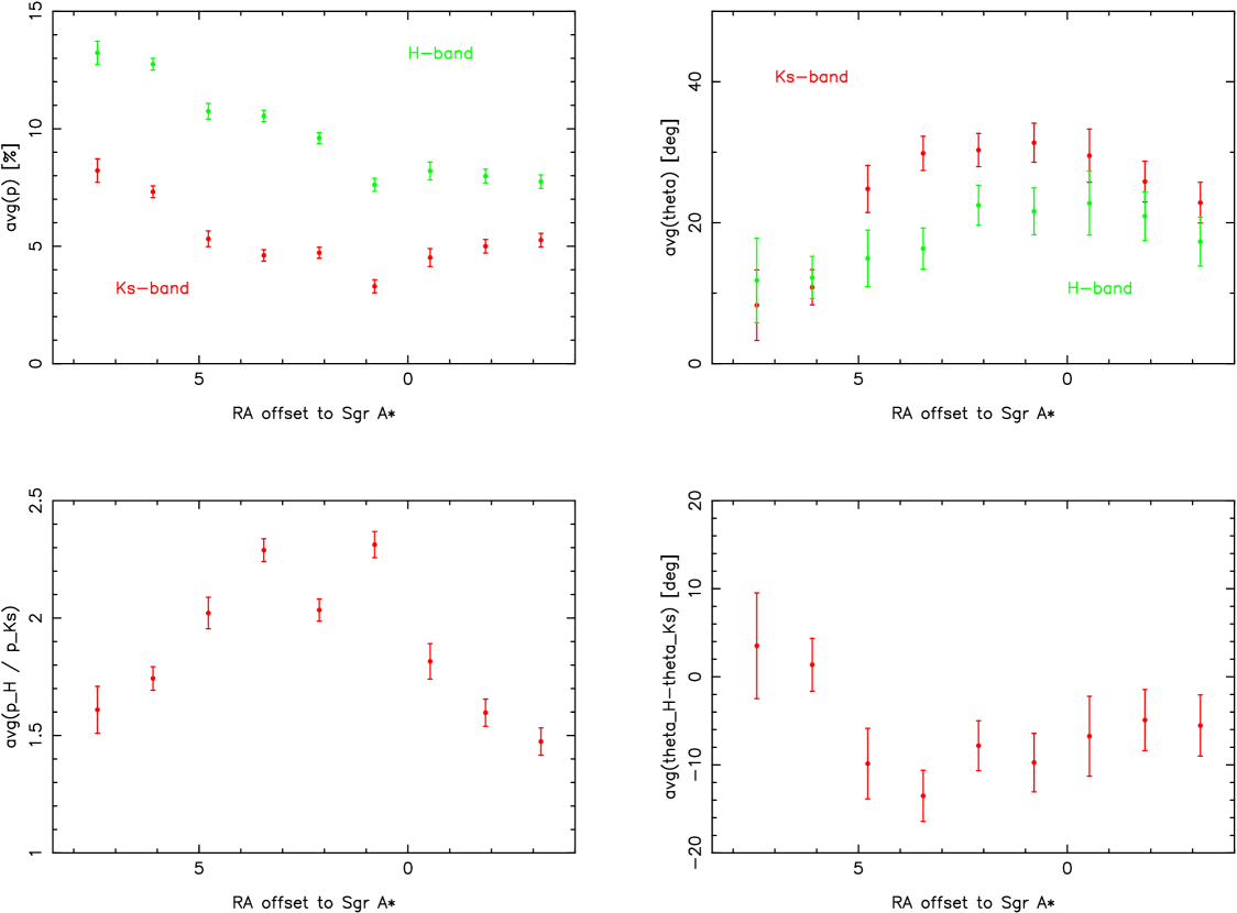
Figure 15: H- and Ks-band polarization parameters, averaged over 1.3” bins along the East-West axis. Upper left: polarization degrees, red: Ks-band, green: H-band. Upper right: polarization angles, red: Ks-band, green: H-band. Lower left: $\frac{p_{H}}{p_{Ks}}$. Lower right: $\theta_{H}-\theta_{Ks}$.

As possible explanations, two basic mechanisms come to mind here:

Variable LOS extinction

The extinction toward the central parsec is known to be ”patchy” (see Schödel et al., 2010b), which in turn indicates different dust column densities and/or dust parameters along individual lines-of-sight toward different regions in the FOV. This could lead to differences in the polarization measured at different locations. But the situation is even more complex. Not only the densities are important, but also possible different alignment in individual dust clouds (so passing through an additional cloud on one LOS compared to another could even lower the total polarization degree for that LOS). Another problem is that we find a smaller effect in the H-band (and thus the impact on $\theta_{H}-\theta_{Ks}$ and $\frac{p_{H}}{p_{Ks}}$). This would require significantly different average dust parameters from one LOS to the other (which in turn requires even more dramatic changes for a considerable percentage of the individual dust clouds along the LOS). Such a configuration is possible, but the highly specific arrangement required to produce a pattern as we observe it seems very unlikely.

Local influences

The area where this effect occurs coincides with the position of a known local feature, the Northern Arm of the Minispiral. This feature is clearly visible in the L-band (see Fig.2), faint in Ks and not detectable in the H-band. The light from the stellar sources itself, which passes through the stream of aligned grains in the Northern Arm, and scattered and/or emitted light from these grains themselves may contribute to some extent to the polarization measured in this region. This would have a stronger impact in the Ks-band compared to the H-band, because of the sizes and temperatures of the involved grains, this far matching our findings. The question however remains how substantial such a contribution could be.
Under conditions as they are found in the filaments, grain alignment by the Davis-Greenstein mechanism would be almost perfect, especially because of the strong magnetic fields (lower limit of $\sim$2 mG close to IRS 1W, see Aitken et al., 1998). By coincidence, the local grain alignment angle in the Northern Arm matches that measured for the LOS polarization (Aitken et al., 1998). This means that local dichroic extinction would increase the observed total polarization degree, while scattering/emission would decrease it (as is indeed found for IRS 1W, see below).
While the trends in polarization degree in the 2009 data may be explained this way, the measured polarization angles do not show the expected behavior: if local and LOS dichroic extinction produce alignment in the same direction, the polarization angles should follow the magnetic field lines (see Fig.5). This is the case between 5” and 1” west of Sgr A*, but farther west, the angles are $\sim 20^{\circ}$ steeper than what would be expected. In the H-band, the angles are less steep in that region, providing a better match to the field lines. The preliminary Ks-band results (March 2011) also seem to agree well with the field. Farther to the south, however, the higher polarization degrees in the 2007 Ks-band data-set occur despite a complicated field structure that does not offer an easy explanation for this effect.
It is questionable whether local dichroic extinction can account for these effects, or if other contributions from scattering or extended emission play a role here. The region observed here is quite complex, with a complicated field structure and gas/dust streams, and in addition, the exact position of the observed sources along the LOS axis is not clear. It is therefore difficult to determine what effect even a given dust distribution with a known temperature and composition would have on a certain source, but not even these parameters are known exactly.
We therefore conclude that local effects, such as local dichroic extinction, extended emission by and scattering on dust grains are the most likely cause for this effect, although we cannot determine the likely extent of the individual contribution from the available data on dust parameters and configurations along the LOS and in the GC itself.
This immediately leads to the next question: are these trends mirrored by the behavior of the extinction measured in the FOV?

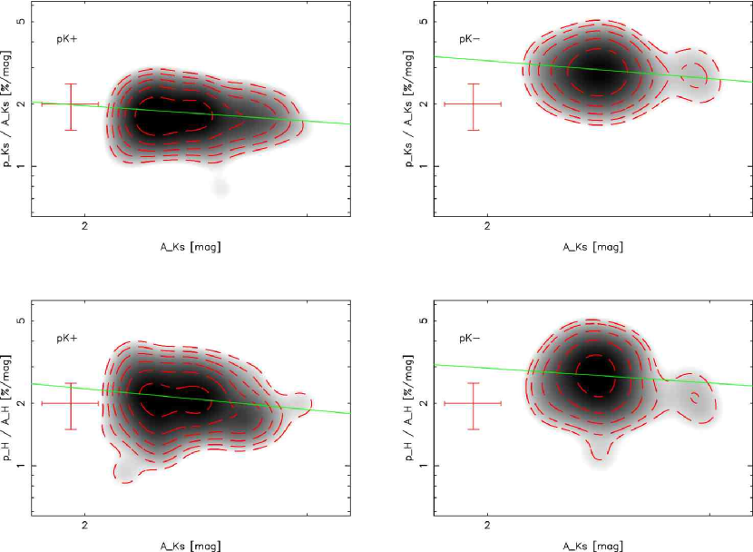
Figure 16: Polarization efficiency in Ks-band (upper frames) and H-band (lower frames), compared to Ks-band extinction, plotted as point density, with typical error represented in upper left corner. pK⁺ and pK^- sources shown separately in left resp. right frames for both bands. Green lines represent the fitted power-law relation.

3.5 Correlation with extinction

We compared the H- and Ks-band polarization values to the extinction map presented by Schödel et al. (2010b). Fig.16 shows the polarization efficiency $\frac{p_{\lambda}}{A_{\lambda}}$ for both bands plotted against the Ks-band extinction $A_{Ks}$ taken from the extinction map at the location of each source. As it turns out, almost the same distribution of $A_{Ks}$ is found for the pK⁺ and the pK^- sources (see Fig.17), which in turn leads to an offset between the two sub-datasets in polarization efficiency. We therefore plot them separately in Fig.16. In both bands, the distributions can be fitted with a power law:

$$\frac{p_{\lambda}}{A_{\lambda}}\propto A_{Ks}^{\beta},$$ (17)

with $\beta_{Ks,-}=-0.4\pm 0.4$ resp. $\beta_{H,-}=-0.6\pm 0.6$ in the H-band for the pK^- sources. Despite the large errors which stem from considerable scatter of the parameters, this matches the relation found by Gerakines et al. (1995) for the Taurus dark cloud and also the results of Whittet et al. (2008) for Ophiuchus (both in the Ks-band). This is not directly comparable, because the GC is obscured by more than one dust cloud with possibly different dust alignments. A more general study by Jones (1989), examining a great number of sources covering a range in optical depth of about a factor of 100, finds a power law relation with $\beta\sim-0.25$. In this study, the author proposed a model where the magnetic field along the LOS consists

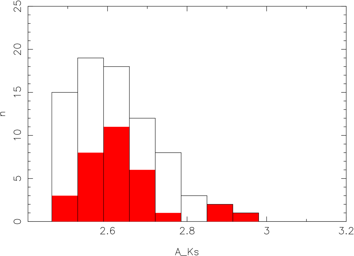
Figure 17: Ks-band extinction for sources with p${}_{Ks}<6$% (open columns) resp. p${}_{Ks}>6$% (filled columns).

of a constant and a random component (see also Heilis, 1987), thus leading to different grain alignment in each section along the LOS. This reproduces the findings in that study quite well, and it is also consistent with our own results within the uncertainties.
For the smaller number of pK⁺ sources, we find similar power law indices: $\beta_{Ks,+}=-0.5\pm 0.7$ resp. $\beta_{H,+}=-0.4\pm 1.5$. Compared to the pH/K^- values, we find a significant offset in polarization efficiency, while the underlying power law appears to be very similar. This might indicate that the additional polarization is indeed caused by a local contribution, likely of Northern Arm material. To produce this deviation along the LOS, a very specific and therefore unlikely dust configuration would be required.

3.6 Examining the extended sources

Our polarimetric data cover two bright extended sources in the central parsec, IRS 1W and IRS 21. The former is contained in both our H- and Ks-band data (datasets 1 and 2), while the latter is covered by several rotated Wollaston datasets of poorer quality (datasets 3-15). IRS 1W shows a clear horseshoe shape as expected for a bow-shock source in high-quality Ks-band images, while IRS 21 does not. Owing to its high apparent polarization, IRS 21 would be interesting as a polarimetric calibration source, but only if the polarization is not variable. To constrain the nature of this source even more, we also conducted a flux variability analysis on IRS 21 and other extended sources in the FOV of our polarimetric data and several NACO imaging datasets, taken between 2002 and 2009 in the H-, Ks- and L-band.

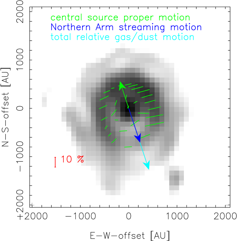
Figure 18: Map of the intrinsic Ks-band polarization of the extended source IRS 1W. The arrows indicate the proper motions of the central source, the motion of the Northern Arm material and the motion of both relative to each other.

3.6.1 IRS 1W

Source morphology

IRS 1W shows the characteristic horseshoe-shape of a bow-shock source (see e.g. Tanner et al., 2005). This shape can already be made out in the raw images, but it becomes even more apparent in a Lucy-Richardson deconvolved image (using a PSF obtained from bright IRS 16 sources, see Fig.18). The observed shape agrees very well with the relative velocities of the streaming material of the Northern Arm (Lacy et al., 1991) at the location of the source and the proper motion of IRS 1W itself (Schödel et al., 2009, , velocities plotted in Fig.18).

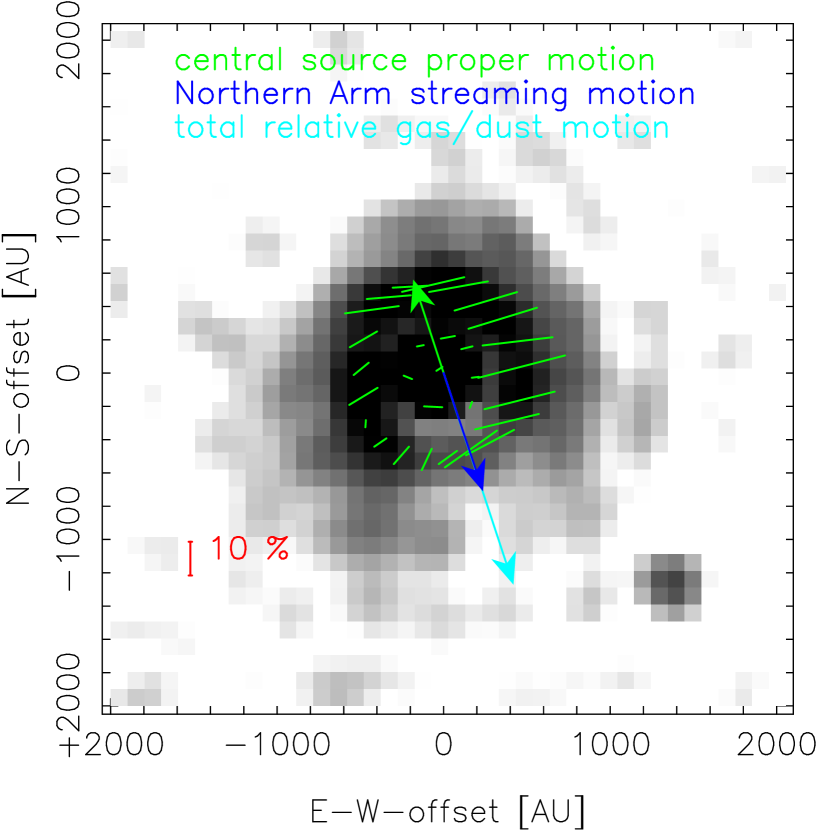
Figure 19: Map of the intrinsic H-band polarization of the extended source IRS 1W (see Fig.18).

Spatially resolved polarimetry

We measured the total polarization of IRS 1W as (1.8 $\pm$ 0.5) % at (-37 $\pm$ 5)^∘ East-of-North after application of the Müller matrix to account for instrumental polarization. Ott et al. (1999) provide values of (4.6 $\pm$ 2.5) % at (-85 $\pm$ 8)^∘ East-of-North. It has to be considered that instrumental effects take place on the same order of magnitude as the measured polarization degree, which may explain the large offset in polarization angle compared to the older values where these effects were not compensated. We attribute our lower total polarization degree to the better angular resolution and thus less influence from neighboring sources. The values provided by Eckart et al. (1995) are clearly influenced by neighboring stellar sources, with (3.0 $\pm$ 1.0) % at (10 $\pm$ 7)^∘.

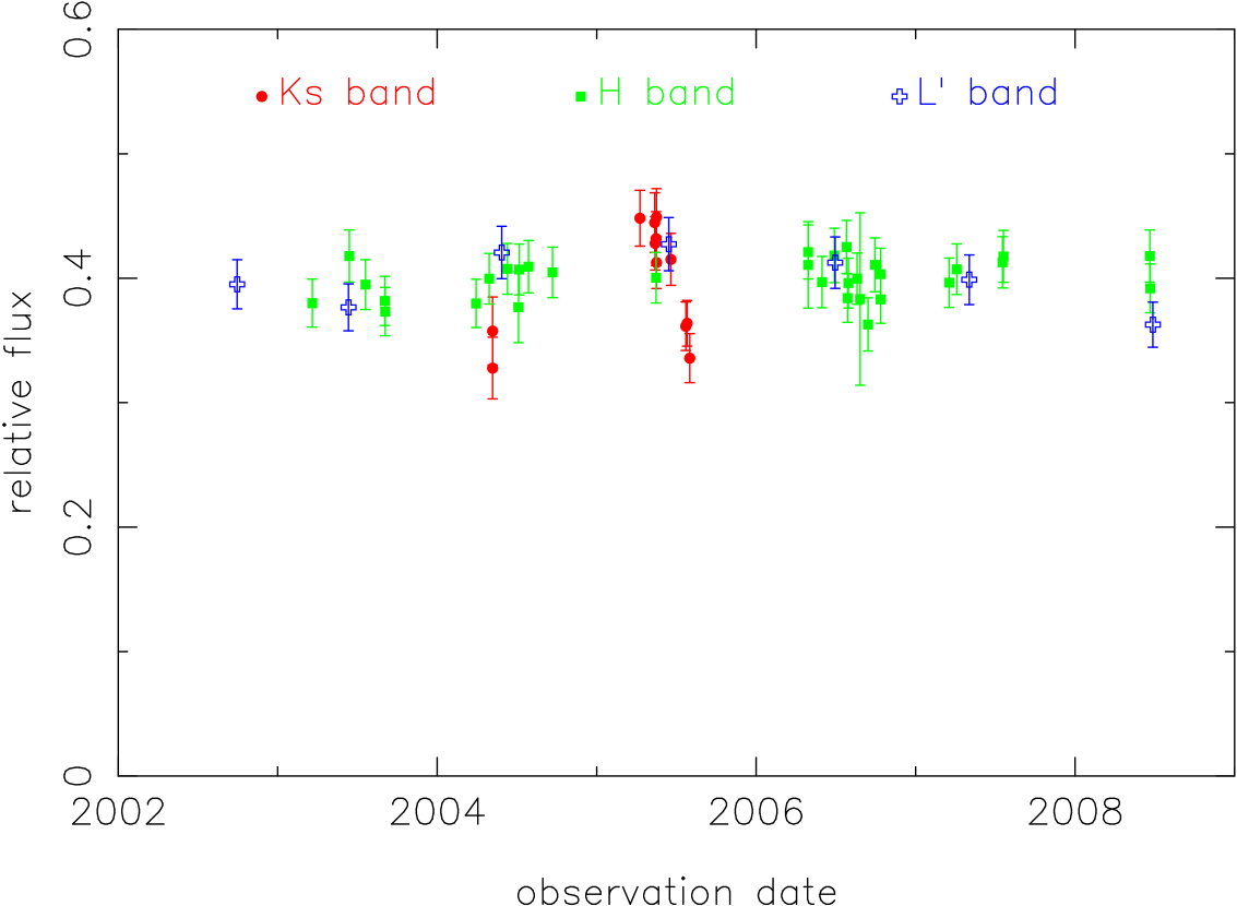
Figure 20: Ks-band (red circles), H-band (green squares) and L-band (blue open crosses) lightcurves of IRS 1W. Shown here is the flux of the source normalized to the flux of non-variable reference sources in the respective band. H- and L-band values were multiplied by a constant factor to match the average Ks-band values.

If we assume that the foreground polarization for this source is the same as for the surrounding objects and apply a depolarization matrix with the parameters for $p=7.6\%,\theta=9.2^{\circ}$, we find a total intrinsic polarization of (7.8 $\pm$ 0.5) % at (-75 $\pm$ 5)^∘.
In the H-band we measured the total polarization of IRS 1W as (5.2 $\pm$ 0.5) % at (12 $\pm$ 5)^∘ East-of-North. The polarization angle appears typical for a stellar source affected by foreground polarization, but the polarization degree is much lower than the $\sim$12% found for stellar sources in the vicinity. We applied a depolarization matrix with $p=12\%,\theta=15^{\circ}$ and found a resulting intrinsic polarization of (6.9 $\pm$ 0.5) % at (-73 $\pm$ 5)^∘. The angle agrees very well with the Ks-band polarization angle, suggesting that the same process is responsible. The lower intrinsic polarization degree points to the lower influence of the extended dust component compared to that of the central source at this wavelength.

Figure 21: IRS 21 observed on 2004-08-30, right: image before Lucy-Richardson deconvolution, left: image after deconvolution (logarithmic gray-scale, contours trace 10, 20, 30, 50, 60, 70, 80, 90, 95% of maximum flux in the left frame, resp. 40, 50, 60, 70, 80, 90, 95, 99% in the right frame.

Figure 22: IRS 21 observed on 2005-05-14, right: image before Lucy-Richardson deconvolution, left: image after deconvolution (logarithmic gray-scale, contours trace 10, 20, 30, 50, 60, 70, 80, 90, 95% of maximum flux in the left frame, resp. 40, 50, 60, 70, 80, 90, 95, 99% in the right frame.

We measured the polarization of individual regions of the source in the deconvolved images and subtracted the foreground polarization using a Müller matrix as described in §2.5. The results are shown in Fig.18. We find polarization degrees of about 10-20 % with very similar polarization angles for regions with significant flux. Apparently, the polarization degree is lower by a factor of up to $\sim$3 around the apex compared to the tails.
We applied the same technique to our H-band dataset, and Fig.19 shows the result for the immediate area around IRS 1W. We find a polarization pattern comparable to that in the Ks-band, with polarization degrees of about 10-20 % with very similar polarization angles for regions with significant flux and much lower polarization degrees in the central region. There is no significantly lower polarization degree toward the apex, as found in the Ks-band, but it has to be noted that the horseshoe shape is much less pronounced in the H-band anyway. The angles agree with those determined from the Ks-band data.
The total intrinsic polarization and the spatially resolved pattern of IRS 1W can be explained from the combination of the motion of the source itself, the streaming velocity of the Northern Arm and the magnetic fields present in that structure.
Aitken et al. (1998) mapped the polarization of the Northern Arm at 12.5 $\mu$m and inferred the magnetic field orientation by assuming that the polarization was produced by emission from magnetically aligned elongated dust grains. The magnetic field at the location of IRS 1W is perpendicular to the polarization angles we find here. The projected velocity of the source (Schödel et al., 2009) is parallel to the field lines and also parallel to the streaming motion in the Northern Arm itself (Lacy et al., 1991). This leads to the field lines following the morphology of the shock around the source. At the apex this causes a weakening of the field, while it is compressed in the tails. This in turn leads to a weaker resp. stronger grain alignment in the apex resp. the tails.
Grain temperatures in the Northern Arm reach up to $\sim$200-300 K (Smith et al., 1990; Gezari, 1992), and this is sufficient to explain the observed 12.5 $\mu$m emission. But for significant emission in the H- and Ks-band, much higher grain temperatures of $\sim$1000 K would be required. This raises the question if the extended emission in the bow-shock is emission from or scattering on the aligned grains. One possibility is that the temperature in the shock is indeed high enough for significant emission. Geballe et al. (2004) suggest that these higher temperatures could be reached by very small grains ($\sim$0.001-0.01 $\mu$m, which is by a factor of 10 smaller than typical grains expected here) if they are heated by occasional high-energy photons or stochastic collisions with high-energy electrons or ions. Moultaka et al. (2004) find that the spectrum measured for IRS 1W (including the bow-shock) matches a 900 K blackbody. At this higher temperature, emission from heated aligned dust grains should contribute to the Ks-band and H-band polarization.

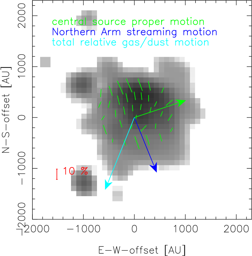
Figure 23: Map of the intrinsic Ks-band polarization of the extended source IRS 21 (see Fig.18).

This leaves the question of the survival of these very small grains in a bow-shock environment and at this temperature. In addition, these grains would have to be aligned to produce the observed polarization. But the very same processes that would heat the small grains to high temperatures would also randomize any previous alignment unless the alignment mechanism is much faster than the randomization. This may be the case here, because strong frozen-in and compressed magnetic fields provide an even stronger and faster alignment than in other regions of the Northern Arm. This might also add to the lower polarization at the apex due to turbulence, which could lead to a partial randomization of grain alignment, before the stronger field and uniform streaming motion in the tails increase the alignment again.
In addition to emission, scattered light from the central source enclosed in a dusty envelope could contribute to the observed polarization. This process is known to occur in planetary nebulae and dusty young stellar objects (YSOs) (e.g. Lowe & Gledhill, 2007; Lucas & Roche, 1998).

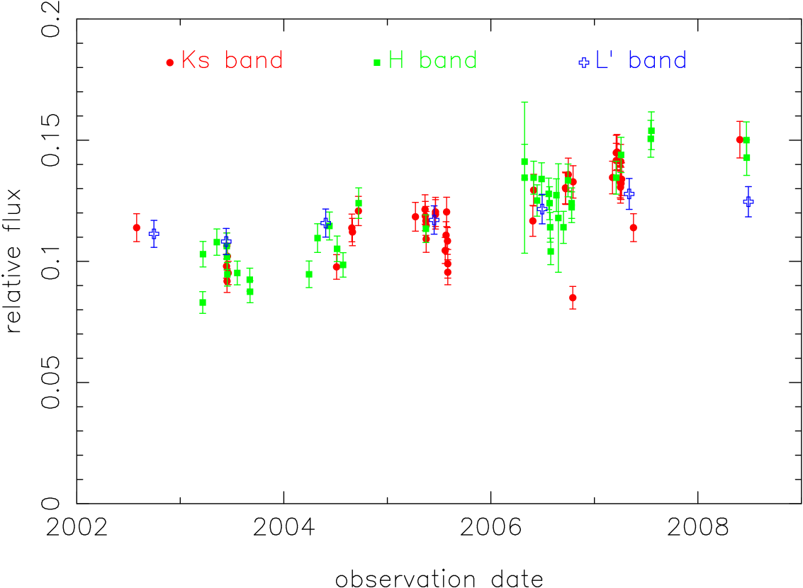
Figure 24: Ks-band (red circles), H-band (green squares) and L-band (blue open crosses) lightcurves of IRS 21. Shown here is the flux of the source normalized to the flux of non-variable reference sources in the respective band. H- and L-band values were multiplied by a constant factor to match the average Ks-band values.

Table 2: Polarization parameters measured for IRS 21. The average over all observations resp. the standard deviation is given in the last line.

	date	p$[\%]$	dp$[\%]$	$\theta$ [deg]	d $\theta$ [%]
1	2007-04-01	10.4	0.5	15	5
2	2007-04-03	9.3	0.5	16	5
3	2007-04-04	8.9	0.5	15	5
4	2007-04-05	8.8	0.5	17	5
5	2007-04-06	9.0	0.5	16	5
6	2007-07-18	9.4	0.5	16	5
7	2007-07-19	9.0	0.5	17	5
8	2007-07-20	9.1	0.5	16	5
9	2007-07-20	9.0	0.5	18	5
10	2007-07-21	8.4	0.5	17	5
11	2007-07-23	9.2	0.5	16	5
12	2007-07-23	8.3	0.5	18	5
13	2007-07-24	9.5	0.5	16	5
avg		9.1	0.2	16.4	0.3

In the ideal case of pure Mie-scattering on spherical dust grains, most of the light would be scattered forward, but a significant portion is scattered perpendicular to the incident direction. This latter part is linearly polarized, with the polarization vector in the plane of the sky and perpendicular to the original propagation direction of the light. If a source like this is viewed face-on, no total intrinsic polarization is detected, because the polarizations of the regions surrounding the central source cancel each other out. If the source is inclined, any total polarization angle can be produced. Spatially resolved polarimetric measurements of these sources show a characteristic centrosymmetric pattern of the polarization vectors, however. Clearly, this is not the kind of pattern we find here.
But what if the grains are not spherical, but elongated and aligned as is the case here at least for a significant part of the grain population? Lucas & Roche (1998) find patterns of aligned polarization vectors similar to the ones we find here in the central regions of a minority of the sources examined in their study. They claim that these patterns cannot be explained by scattering on spherical grains, but that aligned elongated grains must play a role there. Whitney & Wolff (2002) modeled scattering and dichroic extinction for non-spherical dust grains, finding a variety of polarization patterns for different input values for optical depth, degree of grain alignment, and inclination of the source. In general, at low optical depths they find polarization vectors perpendicular to the axis of grain alignment (i.e. the orientation of the angular momentum vector of the spinning grains), while high optical depth leads to a predominance of dichroic extinction and thus to polarization vectors parallel to the axis of grain alignment. This study is focussed on spherical dust configurations and disk-like structures, so the results are not directly applicable to a bow-shock source.

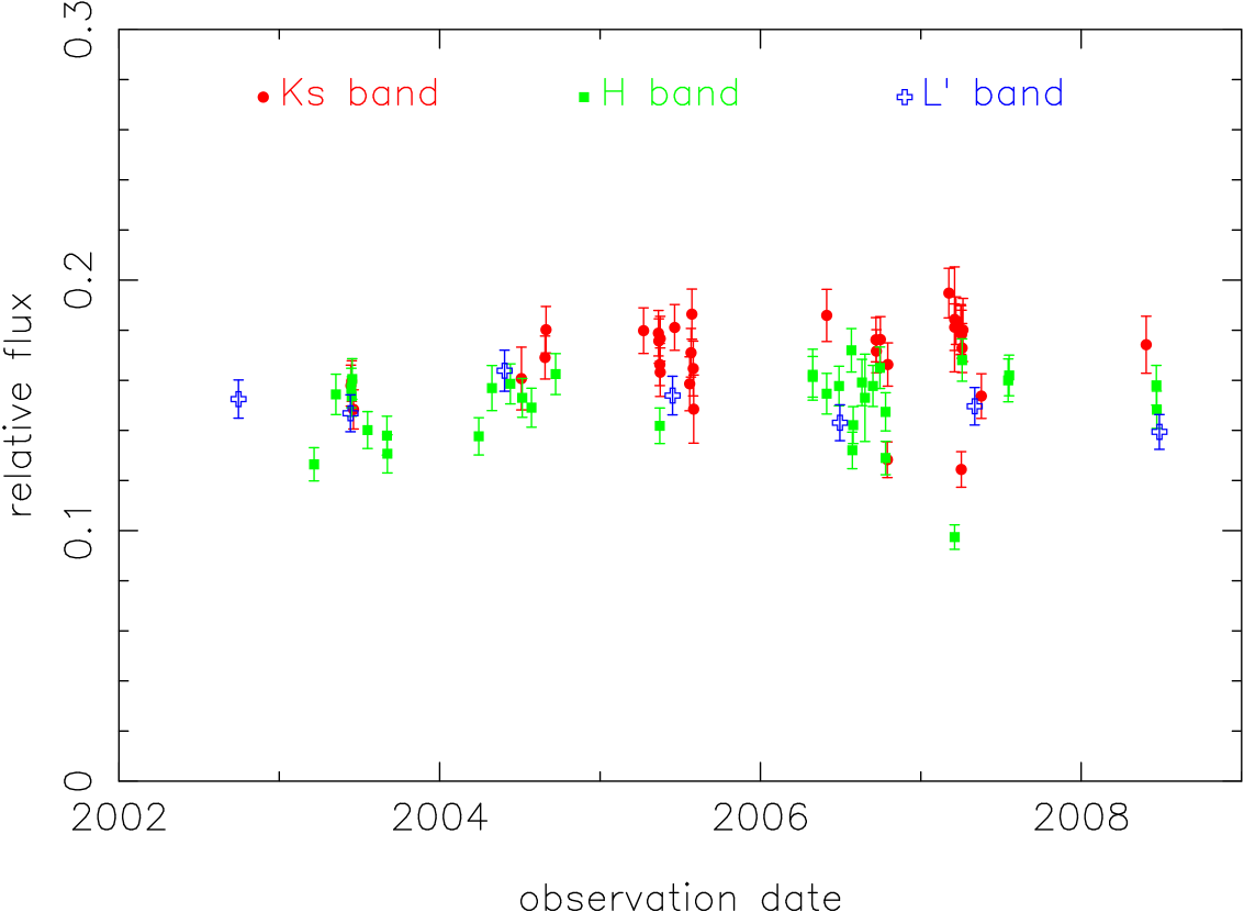
Figure 25: Ks-band (red circles), H-band (green squares) and L-band (blue open crosses) lightcurves of IRS 10W. Shown here is the flux of the source normalized to the flux of non-variable reference sources in the respective band. H- and L-band values were multiplied by a constant factor to match the average Ks-band values.

In the light of these results, we consider it likely that scattering on elongated grains contributes to the observed patterns in the H- and Ks-band data. Both scattering and emission should produce polarization at the same angle. Without thoroughly modeling the conditions in such a bow-shock environment, we cannot conclude which process is dominant, only that both probably contribute.

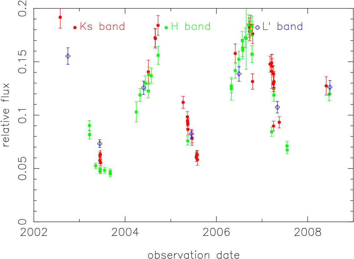
Figure 26: Ks-band (red circles), H-band (green squares) and L-band (blue open crosses) lightcurves of IRS 10E. Shown here is the flux of the source normalized to the flux of non-variable reference sources in the respective band. H- and L-band values were multiplied by a constant factor to match the average Ks-band values.

Flux variability

The total flux of IRS 1W can be difficult to determine, because the center of this source is saturated in many images. Unfortunately, the repairing algorithm included in StarFinder only works on point sources, because it assumes that the saturated source has a PSF similar to that of non-saturated sources in the vicinity. This is obviously not the case for an extended source like IRS 1W. We therefore only used data where the peak fluxes at the location of IRS 1W stayed below the saturation threshold. Fig.20 shows the flux of IRS 1W in relation to the reference flux in the H-, Ks- and L-band. The flux appears to be variable by $\sim$30% in the Ks-band, while the H-band value is inconclusive. No clear periodicity is apparent, which might indicate either an erratic variability or a period on the order of or below the time resolution of our data. The flux variability exceeds that found for IRS 16C (see Fig.4), but this may in part be due to the difficult photometry on IRS 1W. In the L-band, the flux rises to a maximum in 2005 and drops again by $\sim$15 %. We consider this consistent with a constant flux within the uncertainties, especially since there is no correlated behavior over the H-, Ks- and L-band. In total, we cannot state whether or not IRS 1W shows a source-intrinsic flux variability based on the available observations.

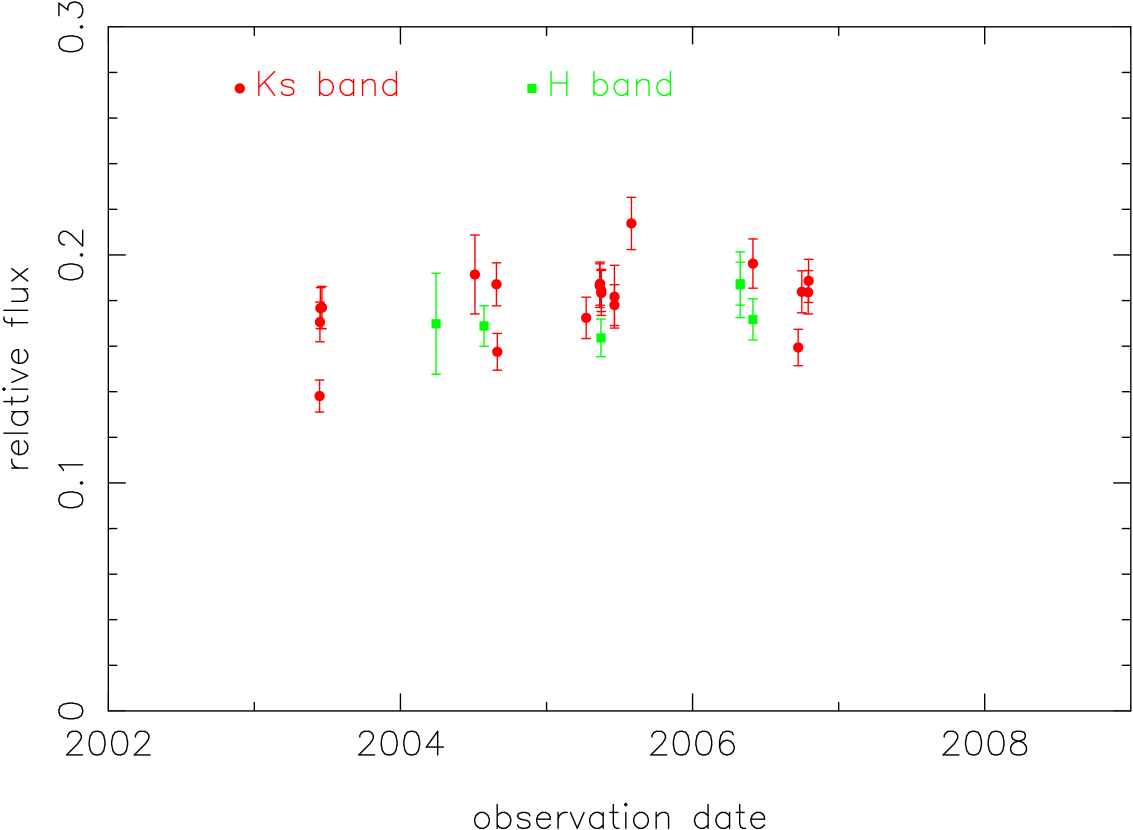
Figure 27: Ks-band (red circles), H-band (green squares) and L-band (blue open crosses) lightcurves of IRS 5. Shown here is the flux of the source normalized to the flux of non-variable reference sources in the respective band. H-band values were multiplied by a constant factor to match the average Ks-band values.

3.6.2 IRS 21

Source morphology

Previous studies show IRS 21 as a roughly circular, yet extended source (Tanner et al., 2002, 2005). We find the same for our data, but after applying a Lucy-Richardson deconvolution, this changes significantly: Fig.21 and 22 show IRS 21 before and after deconvolution for two datasets (2004-08-30 resp. 2005-05-14). There is no clear bow-shock shape visible prior to deconvolution. After the LR process, there is still no clear horseshoe shape, but it is clear that the source is not circular in projection and thus most likely not spherical. The deconvolved images appear to contain a central source with a bow-shaped northern extension. It has to be noted that this shape is not this apparent in all our datasets, but the resolution that can be achieved on an extended feature like this critically depends on the data quality, especially in a very dusty environment like that of IRS 21. The LR algorithm also tends to ’suck up’ flux of extended features into a central source (see Appendix B). For all but a few periods, however, the deconvolved images show an extended structure at this location, with an east-western bar/bow to the north and a point-source-like feature to the south. We deem this shape to be consistent with a marginally resolved bow-shock type source. Our findings match those presented by Tanner et al. (2004), who find a similar spatial structure and position angle of the bow-shock in the L-band. Furthermore, the relative motion of the Northern Arm material Lacy et al. (1991) and the proper motions of IRS 21 (e.g. Tanner et al., 2005) would agree with a bow-shock in this direction (see projected velocities plotted in Fig.23).
From the images where the bow-shock shape was visible, we determined a projected distance between the peaks of the southern and the northern feature of $\sim 400\pm 100$ AU (see Fig.21). The projected distance was almost the same for all images, and the error given here is just a rough estimate. Considering a possible inclination of the source, this constitutes a lower limit for the standoff distance between the central source and the apex of the bow-shock. Tanner et al. (2002) provide modeled standoff distances for candidate central objects, using the Ks-band radius they measure for IRS 21 of $\sim$650 AU as an estimate for the standoff distance. Using the radius makes this value an upper limit for the projected standoff distance. They find that this value agrees best with the following stellar types: an AGB type star, W-R, Ofpe/WN9 or W-R WC9. Especially a Wolf-Rayet (W-R) type star would be able to produce a wide range of possible standoff distances (310-10100 AU). Our value agrees with these possibilities as well.

Spatially resolved polarimetry

IRS 21 is not covered by our main high-quality polarimetric dataset, so we measured its total polarization in several other datasets with lower Strehl ratios (see Tab.3, datasets 3-15, the data quality is still sufficient for polarimetry on bright sources). The values we find for the individual datasets are shown in Tab.2. Considering the uncertainties, we conclude from these measurement that both the polarization degree and angle of IRS 21 can be treated as constant within our margin of error. We find an average value of (9.1 $\pm$ 0.2) % at (16.4 $\pm$ 0.3) degrees, which agrees very well with the polarization measured by Ott et al. (1999) and also with the polarization angle determined by Eckart et al. (1995). The latter study measured a polarization degree which is $\sim$60% higher than our value. Ott et al. (1999) explained this difference by different apertures used and that might indeed be the case. We did not find a clear indication of a variable polarization degree of IRS 21 in the available data, although several, low quality datasets led to some outlier values. Since this coincided with large variations in the polarization of other sources, we do not consider this a significant effect.
After applying a depolarization matrix with polarization parameters determined from the surrounding point sources (5% at 30^∘, determined on two sources close to IRS 21 and thus not as reliable as the values for IRS 1W), IRS 21 appears to have a total intrinsic polarization of (6.1 $\pm$ 0.5) % at (5 $\pm$ 5) degrees. The polarization degree is slightly lower than that of IRS 1W, while both sources have very different intrinsic polarization angles. Again, the angle we find is perpendicular to the magnetic field orientation in this region given by Aitken et al. (1998). Unfortunately no polarimetric H-band data covering IRS 21 is available.
Fig.23 shows the polarization of individual regions. We find polarization degrees of about 3-8 %, with less uniform polarization angles than those found for IRS 1W in regions with significant flux. We also detect an increase instead of a decrease of the polarization degree toward the apex. The polarization angle shows more variation compared to IRS 1W.
Again, the relation of the source motion and the local magnetic fields and streaming motions offer an explanation. The source moves almost perpendicular to the field, so the field lines are likely compressed in front of the shock and diluted toward the flanks. This leads to a higher polarization at the apex. If this field orientation is indeed preserved over the whole structure, it could explain the observed polarization pattern, because the polarization angles would be perpendicular to the field lines. This would be the expected behavior for emission/scattering producing the polarization.
For this grain alignment dichroic extinction would be expected to produce polarization angles perpendicular to what is observed here. This would reduce the overall intrinsic polarization, but it is questionable if the optical depth of the dust surrounding IRS 21 is sufficient for a significant contribution of this process. Again, a detailed model of bow-shock polarization using measurements at different NIR wavelengths as input parameters might clarify the extent of the influence of these processes. For the purposes of this study, we assume that scattering and emission play the dominant role.

Flux variability

Fig.24 shows the flux of IRS 21 in relation to the reference flux. For the H- and the Ks-band data the flux significantly and steadily increases by about 50% over the observed period (June 2002 to May 2008). This corresponds to an increase in brightness of about 0.4 mag. That we find the same increase for both bands suggests that it is intrinsic to the source itself, because the H-band is dominated by the stellar component, while the Ks-band source is dominated by the dust enshrouding the stellar source. We find a lower ($\sim$20%) correlated flux increase in the L-band data as well. What could cause this increase in flux?
From the available data we cannot determine whether this is a periodic variability or not because we only observe a steady increase in flux. This would be possible for all candidates presented by Tanner et al. (2002): both AGB-stars and Wolf Rayet stars may show such an increase in luminosity in this time-frame, especially if they are in a mass-losing phase.

Table 3: Details of the observations used for this work. N is the number of exposures that were taken with a given detector integration time (DIT). NDIT denotes the number of integrations that were averaged online by the read-out electronics during the observation. The Strehl ratio was measured using the Strehl algorithm of the ESO eclipse package (see N. Devillard, ”The eclipse software”, The messenger No 87 - March 1997, publicly available at http://www.eso.org/projects/aot/eclipse/distrib/index.html, given here is the average value over all images in each dataset.

	program	date	band	mode	channels	N/channel	NDIT	DIT[sec]	camera	Strehl
1	073.B-0084(A)	2004-06-12	H	Wollaston	0, 45	30	1	30	S13	0.171
2	083.B-0031(A)	2009-05-18	Ks	Wollaston	0, 45	143	4	10	S13	0.272
3	179.B-0261(A)	2007-04-01	Ks	Wollaston (rotated)	0, 45	15	2	15	S13	0.126
4	179.B-0261(A)	2007-04-03	Ks	Wollaston (rotated)	0, 45	70	2	15	S13	0.217
5	179.B-0261(A)	2007-04-04	Ks	Wollaston (rotated)	0, 45	23	2	15	S13	0.173
6	179.B-0261(A)	2007-04-05	Ks	Wollaston (rotated)	0, 45	70	2	15	S13	0.103
7	179.B-0261(A)	2007-04-06	Ks	Wollaston (rotated)	0, 45	51	2	15	S13	0.138
8	179.B-0261(D)	2007-07-18	Ks	Wollaston (rotated)	0, 45	130	2	15	S13	0.188
9	179.B-0261(D)	2007-07-19	Ks	Wollaston (rotated)	0, 45	70	2	15	S13	0.075
10	179.B-0261(D)	2007-07-20	Ks	Wollaston (rotated)	0, 45	70	2	15	S13	0.084
11	179.B-0261(D)	2007-07-20	Ks	Wollaston (rotated)	0, 45	70	2	15	S13	0.137
12	179.B-0261(D)	2007-07-21	Ks	Wollaston (rotated)	0, 45	51	2	15	S13	0.137
13	179.B-0261(D)	2007-07-23	Ks	Wollaston (rotated)	0, 45	124	2	15	S13	0.079
14	179.B-0261(D)	2007-07-23	Ks	Wollaston (rotated)	0, 45	41	2	15	S13	0.023
15	179.B-0261(D)	2007-07-24	Ks	Wollaston (rotated)	0, 45	30	2	15	S13	0.081

3.6.3 IRS 10

IRS 10W shows a flux variability in all three bands, but there is no clear periodic behavior (see Fig.25, only values not affected by saturation are shown). The Ks- and H-band fluxes vary by about $\sim$30%, while the L-band flux only shows about 10% variability. We do not consider this a reliable detection of intrinsic variability, because no systematic trends are visible at the observable timescale. By comparison, IRS 10E shows a strong and clear periodic variability with the flux increasing by a factor of 3 and a period of about two years (see Fig.26). The variability is correlated in the H-, Ks and L-band. This source has been classified as a late-type Mira variable by Tamura & Werner (1996), while Ott et al. (1999) label it as a long-period variable. Our measurements agree with these classifications.

3.6.4 IRS 5

IRS 5 also shows a flux increase in the Ks-band between 2002 and 2008 (see Fig.27, one value affected by saturation was taken out), although the increase is not as strong and clear as that found for IRS 21. The H-band data is much less clear for this source, and while it appears to be variable at that wavelength as well, the variability seems quite erratic. We therefore cannot conclude that this is an intrinsically variable source on the observed timescale.

4 Conclusions

We draw the following conclusions:

1. Like several previous polarimetric surveys of the central parsec at much lower resolution, we find that the polarization follows the Galactic plane in general. This confirms that the polarization can indeed be attributed to aligned dust grains between the Galactic Center and the observer (foreground polarization). We find systematic and individual deviations from this general pattern, however. Over our FOV we find that the polarization degrees and angles change toward the eastern region around IRS 1. This behavior occurs in the H- and the Ks-band data, with stronger relative deviations in the Ks-band. That can be expected if this is indeed a local effect produced by dust grains in the Northern Arm, because typical temperatures and grain sizes in this region lead to a much more significant impact of radiation from this grain population at longer wavelengths. This is supported by a systematic change of $\frac{p_{H}}{p_{Ks}}$ over the FOV, with values of 2.0$\pm$0.3 in the center and 1.6$\pm$0.3 in the Northern Arm region. The higher of these values leads to a polarization maximum at $\sim 0.7\mu$m, which matches previous findings of $\lambda_{max}\sim 0.8\mu$m by Bailey et al. (1984), based on JHK observations of a more extended region in the GC. This value represents dust parameters, specifically typical grain sizes, and it can be expected that local contributions by distinct dust masses lead to a different value than the average along the LOS. Unfortunately, we cannot derive any more constraints for the local dust based only on these two bands, other than that the dust grains responsible for the local effects must be elongated and aligned (see Aitken et al., 1998), and that their temperature and size must be sufficient for their influence in the H/Ks-band.

2. We find a correlation between the spatially variable extinction toward the central parsec and the polarization efficiency, $\frac{p_{\lambda}}{A_{\lambda}}$. This relation appears to be different for the two groups of sources we find in our FOV (sources only affected by LOS polarization respectively sources where local contributions are significant): for the foreground-polarized sources, we find a power law relation with a similar power law index for the H- and the Ks-band ($\beta_{H}=-0.6\pm 0.6$, $\beta_{Ks}=-0.4\pm 0.4$ ). This is compatible with the measurements resp. the model by Jones (1989), who assume a combination of a constant and a random component of the galactic magnetic field along the LOS to align the dust grains. For the population of higher polarized sources, we find a higher polarization efficiency in general, while the power law index for both bands resembles that of the sources with lower polarization (with $\beta_{H}=-0.4\pm 0.7$ and $\beta_{Ks}=-0.5\pm 1.5$, although it has to be cautioned that these fits are poor because of the small number of sources). The higher polarization efficiency points to the influence of local dust grains, which only contribute a small amount to the total extinction. But because these grains are aligned, they add a significant component to the total polarization, because this alignment is not (partially) compensated by averaging over other dust populations with different alignment as is the case for every individual dust configuration along the LOS. These findings further support our previous conclusion that the influence of local dust is quite significant not only in the MIR, but also in the H- and Ks-band.

3. Intrinsic polarization takes place in several sources in the central parsec, not only at longer wavelengths as shown first by Knacke & Capps (1977), but also in the H- and Ks-band (e.g. Ott et al., 1999). With the Müller calculus we can isolate the intrinsic component for point sources and maps of extended features. The resulting total intrinsic polarization angles for IRS 21 and IRS 1W agree very well with what can be expected from source morphology and relative motion of gas/dust in the Northern Arm and the sources themselves. We find very similar intrinsic polarization degrees for both sources, with (7.8 $\pm$ 0.5) % at (-75 $\pm$ 5)^∘ for IRS 1W and (6.1 $\pm$ 0.5) % at (5 $\pm$ 5) for IRS 21 (both Ks-band). Contrary to the wavelength dependency seen in the foreground polarization, we find a slightly lower H-band polarization degree for IRS 1W compared to the Ks-band: (6.9 $\pm$ 0.5) % at (-73 $\pm$ 5)^∘. That the central source contributes a larger amount of flux in the H-band compared to the extended component, while the intrinsic polarization mostly stems from the bow-shock, explains this discrepancy.
   The spatially resolved intrinsic polarization patterns of both bright extended sources in our FOV do not show a centrosymmetric shape as would be expected for Mie scattering on spherical grains. Instead, the pattern found for IRS 1W suggests that scattering on aligned elongated grains must play a significant role, possibly combined with thermal dust emission (in the Ks-band), because the grains in the bow-shocks may reach temperatures on the order of 1000 K (see Moultaka et al., 2004). Both effects would produce polarization parallel to the long axis of the grains and thus perpendicular to their angular momentum. It therefore appears that the angular momentum of the grains in the bow-shock surrounding IRS 1W is aligned parallel to the relative motion of the source through the Northern Arm material. Taking the magnetic fields in the Northern Arm into account, this is most likely caused by the field lines being warped around the flanks of the bow-shock. This in turn compresses the field lines and thus increases the local field strength, which is then sufficient for fast magnetic alignment of the grains.
   For IRS 21 we find a different polarization pattern. It appears that the polarization vectors are mostly parallel to the relative motion of the source through the surrounding material. Combined with the local field orientation, this again leads to the same dominant mechanism of scattering/emission as for IRS 1W, if we assume that the field lines are compressed in front of the shock that is moving perpendicular to them.

4. After deconvolution, IRS21 clearly does not show a circular shape in the Ks-band. Instead, its shape is consistent with that of a poorly resolved bow-shock with its apex north of the central source. This is consistent with the L-band shape presented by Tanner et al. (2004) and the expectations from the proper motions of the source in relation to the streaming motion of the Northern Arm. We find a standoff distance of $\sim$400 AU, this agrees with the upper limit given by Tanner et al. (2002). It is difficult to constrain the nature of the central source by this parameter alone, and most stellar types with strong winds, such as Wolf-Rayet stars, would be likely candidates (see Tanner et al., 2002).

5. We find a flux variability for several bow-shock sources in the central parsec: IRS 21 shows a flux increase of $\sim$50% over 6 years in the H- and Ks-band (less, but still significant in the Lp-band). Especially the H-band measurement indicates that this variability must be intrinsic to the central source and not only to the envelope. The candidates suggested for the central source by Tanner et al. (2002) could all show this variability, especially a source that is currently in a mass-losing phase.
   While we also find a possible flux variability for IRS 5, IRS 1W, and IRS 10W in all three bands, no clear periodicity or trend is apparent for these sources at our time resolution. We therefore cannot determine if these sources show a true intrinsic variability or not. We confirm the known periodicity of IRS 10E ($\sim$2 yrs) in the Ks-band, finding the same variability in the H- and Lp-band as well.

Several effects appear to contribute to the observed polarization in the central parsec of the GC, in addition to the foreground polarization. The findings in our relatively narrow field-of-view alone indicate possible additional areas of interest: do the large-scale trends we find continue in other sections of the Northern Arm (and the other elements of the minispiral)? Do the other bow-shock sources, such as IRS 10W, 5, and 8 show similar polarization patterns, and what does that tell us about the local processes in the bow-shocks? Are other intrinsically polarized sources present in the field, and what type of objects would show this behavior? More observations with wider FOVs and in different bands (especially L-band, to directly examine extended dust emission e.g. in the Northern Arm) would be desirable, and the recently achieved direct polarimetric calibration of NACO offers the possibility to map more extended areas of the GC in polarization at high resolution.

Appendix A Error estimation

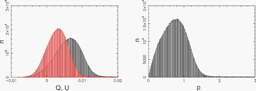
Figure 28: Stokes parameters Q and U (left frame) and resulting polarization degree (right frame), measured for each pixel in a wiregrid flat-field.

In general, several effects can contribute to the total flux uncertainty: the basic uncertainty in the counts measured for each pixel, the insufficiently determined PSF (resp. the fact that a PSF determined from several bright sources does not fit every source perfectly) and possible effects of insufficient calibration (e.g. errors in the sky or the flat-field).
When using StarFinder, the formal flux error given by the algorithm represents the first of these three contributions. The algorithm assumes an independence of all the pixels resp. their measured counts, however. This is not the case anymore for a deconvolved image. Schödel (2010a) circumvented this problem by introducing a modification factor for these formal errors (determined by simulations). Owing to the different instrument setup used here, we could not simply adopt the same factor.

Figure 29: Stokes parameter Q measured at each pixel of a flat-field taken with (upper frames) and without (middle frames) the Wollaston prism. The lower frames show Q after dividing the Wollaston flat-field by the flat-field taken without the Wollaston. Left frames: H-band, right frames: Ks-band.

The second contribution stems from a variation of the PSF over the FOV. Generally, the shape of the PSF changes with the relative position of the source to the guide star (anisoplanasy), with longer projected distances leading to larger distortions. The extent of this behavior is highly dependent on the data quality resp. the seeing. The correlation factor provided by StarFinder describes this effect, because it measures how well a source matches the PSF, but it is not clear how to translate this into a flux uncertainty. We therefore estimated this effect in another way: we extracted three different PSFs from the western, central, and eastern region of the FOV and used them for PSF fitting with StarFinder. As it turned out, this does not only produce different fluxes in all four channels, but can also lead to a shift in polarization angle and/or degree (depending on the source). A similar effect can be seen when comparing fluxes and polarization parameters measured in different sub-frames of the deconvolved image.
We compared these measurements to aperture photometry applied to two bright sources (IRS 16C, IRS 1C). The results are shown in Figs.30,31. In general, we find that the values determined by aperture photometry are matched better by the PSF-fitting values the closer the PSF reference sources are to the source in question. The deviations can reach values of up to 1.5% resp. 10^∘ even for these bright sources.

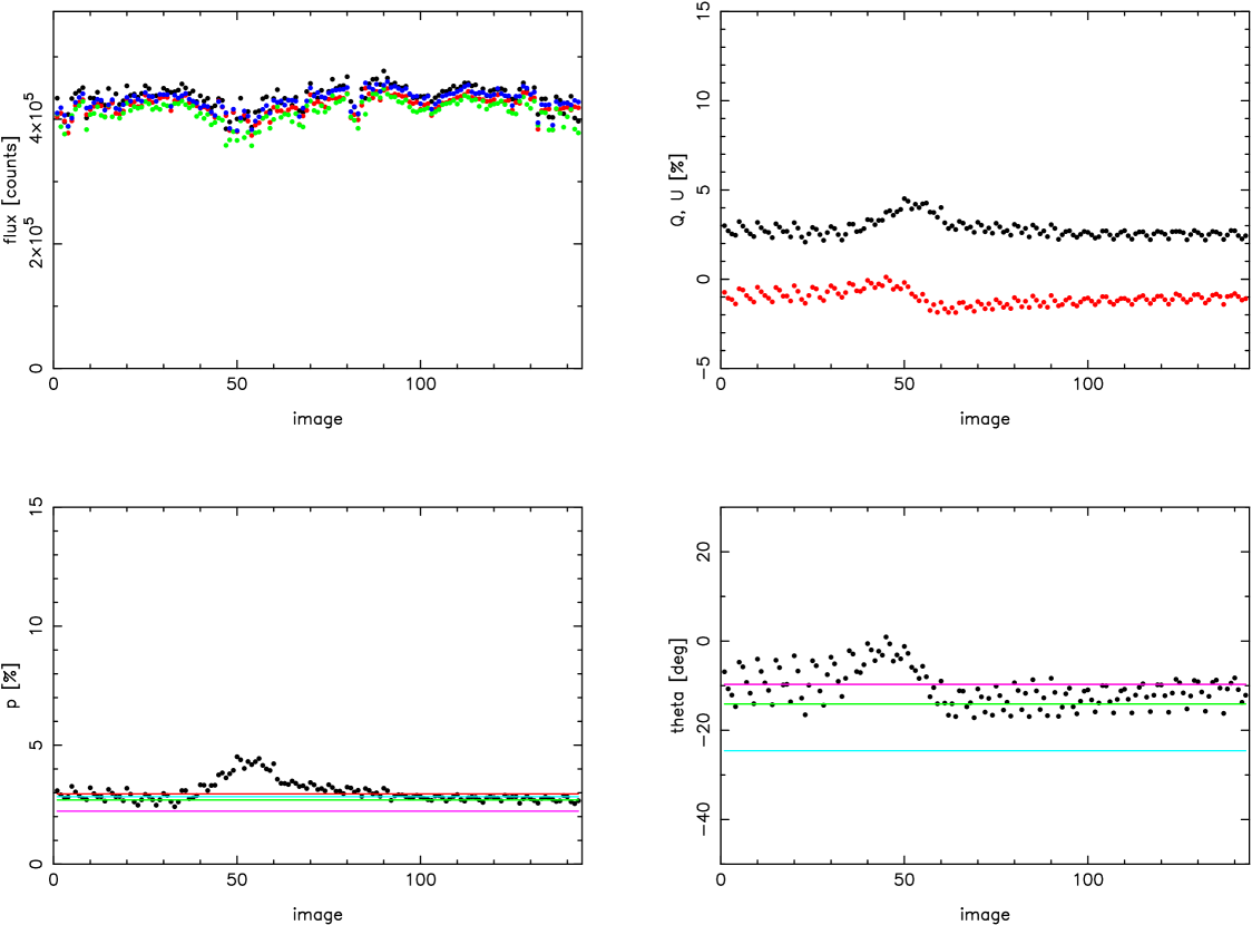
Figure 30: Fluxes and polarization parameters of IRS 16C plotted against time of observation. Upper left: flux measured in four channels. Upper right: Q (black) and U (red). Lower left: polarization degree. Lower right: polarization angle. The plotted lines represent the polarization parameters obtained on the complete mosaic by aperture photometry (red), PSF fitting photometry using the IRS 16 stars (light blue) resp. the IRS 1 stars (magenta), resp. the final value after deconvolution assisted PSF fitting photometry (green).

The reason for this behavior is revealed by a closer look at the individual PSFs: these show a polarization themselves, and that pattern changes over the FOV (see Fig.33, the polarization vectors are almost perpendicular in several locations, even in areas with significant flux). This leads us to conclude that the fluxes determined with a ”nearby” PSF are more accurate than those determined with a ”distant” PSF, and we therefore apply a weighted average (based on the distance of the individual source to the average position of the PSF stars) to the photometry on the deconvolved sub-images. The results provide a better match to the aperture photometry (though it has to be cautioned that the latter is problematic in crowded regions and where large-scale extended emission is present, which is why this method is not applied to the image as a whole). The standard deviation of the fluxes over the sub-frames provides an estimate for the contribution of this effect to the total uncertainty.
Using these error contributions to estimate the final, total uncertainty is problematic: the sub-frames are all taken from the same mosaic and are thus not independent measurements, the formal errors given by StarFinder are unreliable and generally far too small for brighter sources, and possible calibration problems (sky, flat-field) are not covered at all.
We therefore used a different approach to determine the total flux errors: we applied the same photometric method that we used on the full mosaic to mosaics created from eight (Ks-band) resp. six (H-band) sub-datasets, selected based on the dither position along the East-West axis. This led to sub-sets of about 15 (Ks-band) resp. 5 (H-band) images per dither position, and the resulting mosaics have the same depth resp. signal-to-noise ratio everywhere. Because the original images can be regarded as independent measurements, so can the resulting mosaics, with the additional advantage that fainter stars still have a sufficient signal-to-noise ratio (as compared to individual images). The downside of this approach is that all sources in the eastern- and westernmost $\sim$2” are contained in only one of these sub-mosaics. We then adopted the standard deviation of the fluxes measured in these sub-mosaics as the photometric error of each source.
In several cases (mostly in the H-band) this method yielded extremely small errors for weak sources (see Fig.3). This can happen by coincidence if a source is only contained in a small number of sub-mosaics. We consider these errors (and the photometry of these sources in general) unreliable, and the respective source will have a tendency not to pass the reliability criterion for the polarimetry.
The aperture photometry applied to individual frames shown e.g. in Fig.30 reveals two other effects: the measured flux varies over the frames, and in addition to the instrumental polarization (most prominently the ”bump” in p), small variations in Q and U (and subsequently p and $\theta$) can be observed. These variations correspond to the dither pattern used in the observation, and they probe the different areas of the Wollaston prism resp. the detector. These deviations are much smaller than the photometric errors, however, so we assume that we can safely neglect resp. average over them.
Witzel et al. (2011) determined the system-intrinsic systematic uncertainty of polarimetric observations with NACO as 1% in polarization degree and 5^∘ in polarization angle. For a source with 5% polarization (a typical value for GC sources in the Ks-band), this already corresponds to a relative error of 20%. We simulated the required accuracy of the photometry so that the final polarimetric errors stay below three times (resp. six times for the H-band) the systematic uncertainty.

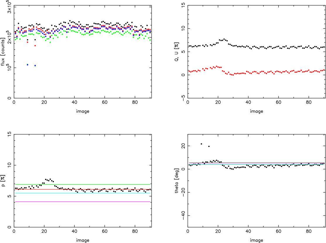
Figure 31: Fluxes and polarization parameters of IRS 1C plotted against time of observation. Upper left: flux measured in four channels. Upper right: Q (black) and U (red). Lower left: polarization degree. Lower right: polarization angle. The plotted lines represent the polarization parameters obtained on the complete mosaic by aperture photometry (red), PSF fitting photometry using the IRS 16 stars (light blue) resp. the IRS 1 stars (magenta), resp. the final value after deconvolution assisted PSF fitting photometry (green).

We tolerate higher uncertainties in the H-band because the higher polarization there leads to a lower relative error for the same absolute uncertainty of the polarization degree. This led to error thresholds of 3% in the Ks-band and 6% in the H-band. Most of the sources brighter than 16 resp. 18 mag (Ks/H) have errors below these thresholds (see Fig.3). This leads to the final error of the polarization parameters being dominated by the statistical photometric errors.

Appendix B LR deconvolution: useful for extended structures?

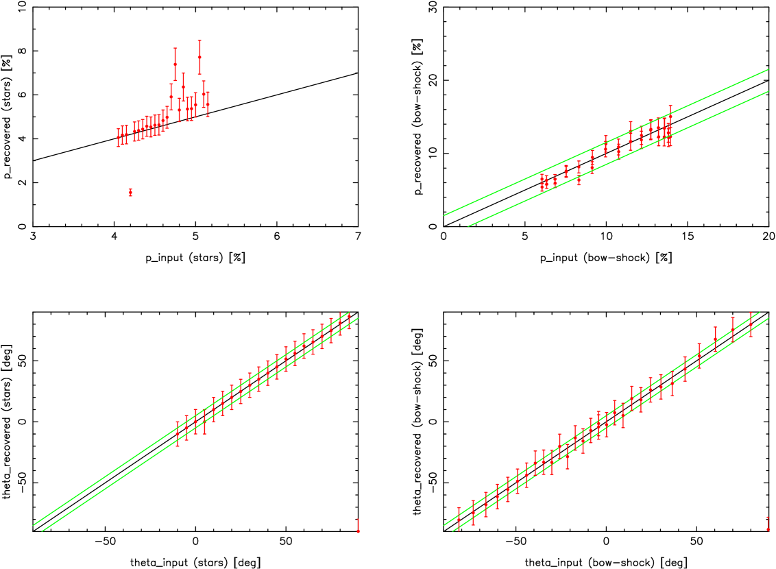
Figure 32: Recovered polarization parameters for point sources (left frames) and extended feature (right frames). The green lines indicate a deviation of $\pm$1.5% resp. 5^∘ from a perfect recovery, indicated by the black line.

It is known that Lucy-Richardson deconvolution has a tendency to ”suck up” surrounding flux into a central point source (see e.g. Schödel, 2010a). This impedes or severely hinders the detection of faint sources close to bright ones, introduces astrometric and photometric uncertainties and makes a reliable background estimation impossible. But unlike linear deconvolution, this method allows flux measurements on extended structures via simple aperture photometry on the deconvolved images. Can it be used to measure the polarization of the extended sources in the GC?
To investigate this, we produced images of an artificial bow-shock-like structure next to a point source. Several other point sources with different fluxes were added to simulate a crowded field as is found in the GC. For each filter (0^∘, 45^∘, 90^∘ and 135^∘), we modified all fluxes by a factor calculated for generic polarization parameters of P = 4-5% and $\delta$ = -10^∘-100^∘:

$$f_{pol,rel}=1+P\times cos(\theta-\delta),$$ (18)

This was applied to the extended feature as well, with a constant polarization degree of 10% and the polarization angles parallel to the bow-shock structure. We then added an additional foreground polarization of 4% at -15^∘ to the extended feature. The resulting map was convolved with a PSF extracted from the real images. We also added a weakly position-dependent background in the shape of a very flat two-dimensional Gaussian similar in level to that found in the actual observations.

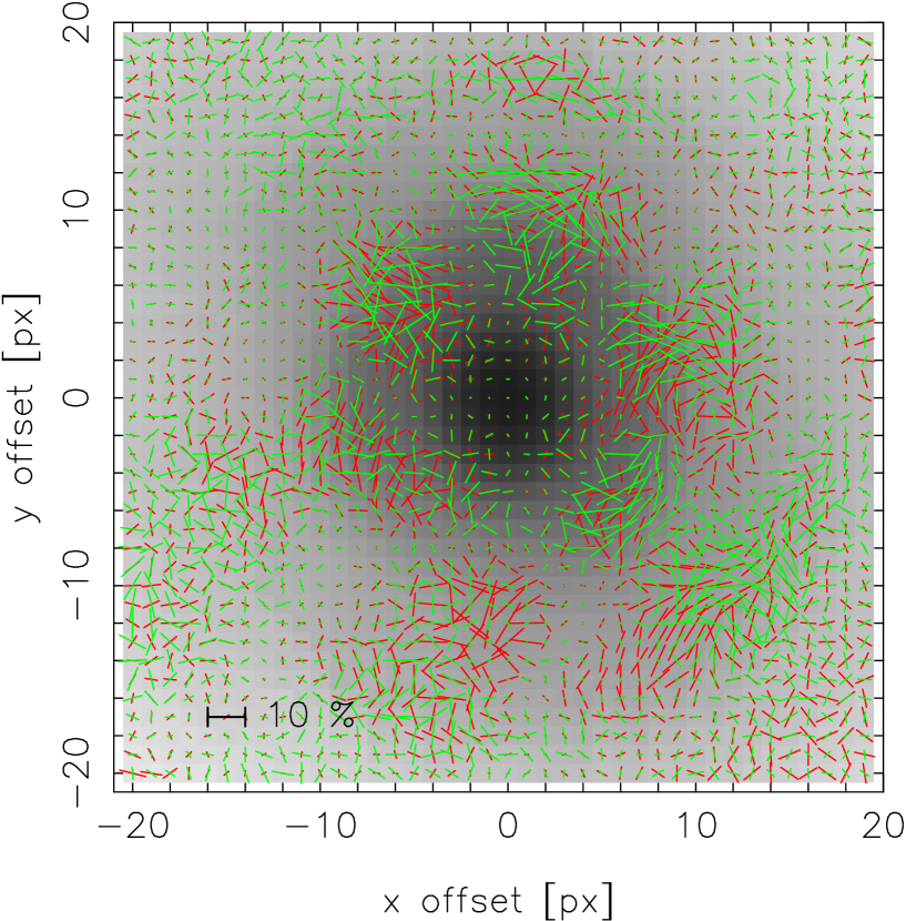
Figure 33: Polarization pattern of the PSF used for the first step of the deconvolution-assisted photometry. Red: PSF determined from IRS 16 sources. Green: PSF determined from IRS 1 sources.

We applied the Lucy-Richardson deconvolution algorithm to these artificial images, followed by aperture photometry on the point sources and the extended structure, mapping the latter with two pixel apertures along its length. The structure itself was successfully recovered, although slightly widened. Fig.32 shows a comparison of the recovered polarization parameters in comparison to the input values. It appears that the only significant large deviation occurs for the source in the center of the extended feature: the recovered polarization degree is 2.6 percentage points lower than the input value, while the polarization angle is 5^∘ less. This appears to be an effect of the algorithm ”sucking” flux of the extended feature into the central source, thereby changing its polarization because of the significantly different polarization of the shell. The polarization degrees of several of the very faint point sources were also recovered poorly, while at the same time their recovered polarization angles agreed much better with the input values.
The values recovered for the bow-shock-feature itself show only small deviations compared to the input values, with a maximum difference in polarization degrees of 1.5-2% (smaller in most cases) and 5-7^∘ in polarization angle. The deviations are even smaller for the brighter stars, with less than 0.5% and less than 1^∘ in most cases. The fainter stars show only slightly larger deviations. This approaches the systematic uncertainties inherent to the instrument. We can therefore consider the Lucy-Richardson algorithm to be sufficiently accurate for our purposes of detecting extended features. The small variances found for the artificial ”bow-shock” also indicate the level of accuracy that can be expected for the polarization parameters determined in §3.6.
Fig.33 shows the polarization pattern of two PSFs determined from different bright sources in the FOV (IRS 16 and IRS 1 point sources). There are significant spatial variations, so these variations must occur (to some extent) in all sources in the non-deconvolved images. Because these sources are expected to be essentially point-like before their light enters the atmosphere, polarization patterns like this must be introduced by instrumental or atmospheric effects. This is another reason why deconvolution is an important step to recover polarization patterns of extended sources successfully: the intrinsic patterns would otherwise be masked by the strong spatial variations, with local values for the polarization degree of up to 15% in the PSF pattern (although these values are much lower in the central region with the highest flux, on the order of 1-2%). These effects are removed by the deconvolution process.